Benchmark Problems for the One-Dimensional Wave Equation Under Mixed Boundary Conditions: Initial-Value and Two-Time Specifications

Abstract

This paper presents two complementary classes of analytical benchmark problems for the one-dimensional wave equation governing longitudinal vibration of a prismatic rod with mixed (clamped–free) boundary conditions. The first benchmark class consists of classical initial-value problems and includes both compatible and incompatible initial data at the space–time corners, highlighting their influence on convergence, regularity, and termwise differentiation of displacement, velocity, and axial force series representations. The second benchmark class prescribes the displacement at two time instants (initial and final time), leading to a fundamentally different modal structure and revealing spectral conditioning effects governed by the ratio $L/\left(c{t}_e\right)$. The derived closed-form solutions provide reference configurations for verification of transient numerical solvers, particularly in scenarios where classical smooth compatibility assumptions are not satisfied.

1. Introduction

The development of high-order p- and $hp$-version finite element methods for transient elastodynamic problems requires analytical benchmark configurations that are suitable for systematic verification. In particular, space–time and variational formulations call for reference problems that extend beyond the classical Cauchy-type initial-value setting.

The one-dimensional wave equation for longitudinal motion in an elastic rod is a classical model in structural dynamics and wave mechanics, and it has long served as a transparent setting for both analytical studies and numerical verification. For mixed boundary configurations, several works have addressed explicit solution formulas and the behavior of formal series representations; see, for example, Korzyuk et al. [1], Anikonov and Konovalova [2], Khromov [3], and Kornev and Khromov [4]. Related analytical viewpoints based on spectral and transform techniques for finite-interval evolution problems and mixed boundary-value settings were also developed by Fokas and Smith [5], by Li and Yu [6], and by Batal et al. [7]. Broader analytical foundations can be found in the classical monographs of Graff [8], Achenbach [9], and Courant and Hilbert [10].

In computational mechanics, closely related bar- and rod-wave problems have also been used extensively to assess numerical methodologies, including meshless and finite element formulations [11]. This connects naturally to studies on finite element discretization and mesh refinement for elastic wave propagation [12], as well as to comparative analyses of spectral and finite-difference approximations for initial-boundary value problems [13]. Even in one spatial dimension, mixed boundary conditions combined with low-regularity initial or boundary data may generate sharp gradients and oscillation-prone regions, making such problems particularly useful for verification. In this context, rod-wave benchmarks have been employed in the study of numerical dissipation, dispersion, and stability [14], and the importance of reliable reference solutions was already emphasized in early finite element studies of transient phenomena [15,16]. Related issues also appear in practical error analysis for the one-dimensional wave equation with non-smooth data [17], in comparisons of spectral and finite-difference schemes [13], and in the analysis of stability and boundary treatment for finite-difference discretizations of wave problems [18,19,20]. From a broader verification perspective, exact or well-defined analytical solutions remain essential for assessing the accuracy and robustness of computational methods [21,22], in agreement with general benchmark concepts used in computational wave problems [23].

Simple rod-wave models are also motivated by applications including impact-type loading, wave propagation in rods interacting with external media, and longitudinal waves generated by damage or loss of support in rod-like structures. Closely related one-dimensional settings with impact-type loading and nonsmooth initial data have been studied analytically by Korzyuk and co-workers [24,25]. These examples further support the use of analytically tractable rod-wave configurations as verification benchmarks.

Recent contributions published in Applied Sciences confirm the continued interest in transient wave propagation and elastodynamic computations using advanced numerical frameworks. Khanal et al. [26] proposed a hybrid modeling strategy for one-dimensional wave propagation, combining different computational approaches for improved efficiency in transient analysis. Yue et al. [27] investigated transient acoustic wave propagation using a time-discontinuous Galerkin finite element formulation, while Liu et al. [28] developed a meshless generalized finite difference framework for elastic wave simulations. Related work on higher-order finite element approximations and dynamic error estimation likewise highlights the importance of reliable reference solutions for systematic verification [29]. At the same time, studies of one-dimensional wave equations with inhomogeneous boundary conditions [30] and analytical investigations of mixed hyperbolic problems [2] show that explicit solution structures are available, even if they are not primarily organized as benchmark families for verification.

A further motivation comes from recent variational approaches to elastodynamics, which allow a broader range of admissible temporal prescriptions than the conventional specification of displacement and velocity at the initial time; see, for example, Tóth [31,32]. This viewpoint is closely related to the long development of time-domain and space–time finite element formulations, beginning with early work on finite elements in time and space [33] and continuing with mixed and variational approaches for transient dynamics [34,35,36,37]. Analytical and semi-analytical treatments of initial-boundary-value problems for wave-like equations have also remained useful in this context [38]. Early studies on time-dependent finite element analysis and variational time integration [15,39], as well as later developments in space–time finite elements [40,41] and hybrid or discontinuous time discretizations [42], all point to the need for benchmark problems tailored to transient and non-classical temporal settings. This need becomes especially clear when one wishes to compare formulations that differ not only in approximation order, but also in their treatment of boundaries, non-smooth data, and conditioning [13,17,20].

In parallel with these numerical developments, a broad spectrum of refined rod theories has been developed over more than a century, extending the classical one-dimensional wave equation by incorporating additional physical effects such as radial inertia, shear deformation, and multimodal kinematics. Classical and higher-order theories—including Rayleigh–Love, Bishop, and Mindlin-type formulations—can be viewed as successive approximations of the three-dimensional elasticity solution of Pochhammer and Chree. A recent review by Elishakoff and Tharu [43] systematizes these developments and provides a unified comparison of classical and refined longitudinal rod models. Nevertheless, most of this literature focuses on physical refinement and dispersion properties rather than on the systematic construction of analytically tractable benchmark problems for verification. Similarly, an extensive literature exists on absorbing, radiation, and transparent boundary conditions for wave simulations [44,45,46], but these studies pursue objectives different from the present one, namely the construction of closed benchmark families with explicit modal solutions under mixed physical boundary conditions.

Against this background, the aim of the present work is to introduce two complementary classes of analytical benchmark problems for the one-dimensional wave equation with mixed (clamped–free) boundary conditions. The first class consists of classical initial-value problems and includes both compatible and incompatible initial data at the space–time corners. The second class prescribes the displacement at two time instants, at the initial and at a specified final time, which leads to a fundamentally different modal structure and reveals parameter-dependent spectral conditioning effects governed by the ratio $L/\left(c{t}_e\right)$. Together, these benchmark classes provide a structured verification framework for transient numerical solvers operating under different temporal prescription types.

While the present manuscript does not propose a new constitutive model, nonlinear wave theory, or metamaterial formulation, its novelty lies in the systematic construction of analytically closed benchmark families tailored to mixed boundary conditions and two distinct temporal prescription types. In particular, the paper places classical initial-value problems and non-classical two-time displacement specifications into a unified framework and makes explicit the roles of corner compatibility, modal coefficient decay, and parameter-dependent spectral conditioning. The resulting benchmark families are intended for the verification of transient numerical solvers, especially high-order and space–time discretizations, in regimes where compatibility and conditioning effects are essential.

2. Governing Equation and Mixed Boundary Conditions

We consider a straight, prismatic elastic rod of length $L>0$ and constant cross-sectional area $A>0$. The material is assumed to be homogeneous and linearly elastic, characterized by Young’s modulus $E>0$ and mass density $\rho >0$. The motion is restricted to longitudinal deformation along the axial coordinate $x\in (0,L)$.

Let $u(x,t)$ denote the axial displacement field at position x and time $t\in (0,t_e)$, where $t_e>0$ is a prescribed final time. In the presence of an axial body force density $f(x,t)$, Newton’s second law applied to an infinitesimal rod element yields

$$EA{\displaystyle \frac{{\partial }^{2}u}{\partial x^2}}(x,t)+f(x,t)=\rho A{\displaystyle \frac{{\partial }^{2}u}{\partial t^2}}(x,t),(x,t)\in (0,L)\times (0,t_e).$$

(1)

In the absence of body forces, that is, for $f(x,t)\equiv 0$, Equation (1) reduces to the one-dimensional wave equation

$${\displaystyle \frac{{\partial }^{2}u}{\partial t^2}}=c^2{\displaystyle \frac{{\partial }^{2}u}{\partial x^2}},c^2={\displaystyle \frac{E}{\rho }},$$

(2)

where c denotes the longitudinal wave speed.

The axial force (normal force) associated with the deformation is given by

$$N(x,t)=EA{\displaystyle \frac{\partial u}{\partial x}}(x,t),$$

(3)

and the particle velocity is

$$v(x,t)={\displaystyle \frac{\partial u}{\partial t}}(x,t).$$

(4)

2.1. Spatial Boundary Conditions

Throughout this work, mixed boundary conditions are imposed. The left end of the rod is clamped, while the right end is subjected to a prescribed axial force. Thus,

$$\begin{array}{cc}\hfill u(0,t)& =\tilde{u}\left(t\right),\hfill \end{array}$$

(5)

$$\begin{array}{cc}\hfill EA{\displaystyle \frac{\partial u}{\partial x}}(L,t)& =\tilde{F}\left(t\right),\hfill \end{array}$$

(6)

for $t\in (0,t_e)$, where $\tilde{u}\left(t\right)$ and $\tilde{F}\left(t\right)$ are given boundary data. In the benchmark configurations considered below, $\tilde{u}\left(t\right)$ will typically vanish, while $\tilde{F}\left(t\right)$ may either be zero or prescribed as a known function of time.

2.2. Temporal Prescriptions

Two types of temporal specifications are considered in this study.

2.2.1. Initial-Value Problems

In the classical formulation, the displacement and velocity fields are prescribed at the initial time,

$$\begin{array}{cc}\hfill u(x,0)& =u_0\left(x\right),\hfill \end{array}$$

(7)

$$\begin{array}{cc}\hfill {\displaystyle \frac{\partial u}{\partial t}}(x,0)& =v_0\left(x\right),\hfill \end{array}$$

(8)

for $x\in (0,L)$.

2.2.2. Final-Value Problems

Alternatively, the displacement may be prescribed at both the initial and a final time instant,

$$\begin{array}{cc}\hfill u(x,0)& =u_0\left(x\right),\hfill \end{array}$$

(9)

$$\begin{array}{cc}\hfill u(x,t_e)& =u_1\left(x\right),\hfill \end{array}$$

(10)

for $x\in (0,L)$. In this case, the temporal prescription differs from the classical Cauchy-type setting and leads to a modified modal structure, as shown in subsequent sections.

The strong form of the problem is therefore defined by Equation (2), together with the mixed spatial boundary conditions (5) and (6) and one of the above temporal prescription types.

3. Benchmark Class I: Initial-Value Problems

In this section, classical initial-value formulations of the longitudinal wave equation are examined under the mixed boundary conditions introduced previously. These problems constitute the first benchmark class and provide analytical reference solutions for the verification of transient numerical schemes. Particular attention is given to the influence of compatibility between initial and boundary data on the structure of the solution.

The governing equation is the homogeneous wave equation

$${\displaystyle \frac{{\partial }^{2}u}{\partial t^2}}=c^2{\displaystyle \frac{{\partial }^{2}u}{\partial x^2}},(x,t)\in (0,L)\times (0,t_e),$$

(11)

where $c^2=E/\rho$.

The spatial boundary conditions are

$$\begin{array}{cc}\hfill u(0,t)& =0,\hfill \end{array}$$

(12)

$$\begin{array}{cc}\hfill EA{\displaystyle \frac{\partial u}{\partial x}}(L,t)& =0,\hfill \end{array}$$

(13)

for $t\in (0,t_e)$.

The initial conditions are prescribed in classical Cauchy form,

$$\begin{array}{cc}\hfill u(x,0)& =u_0\left(x\right),\hfill \end{array}$$

(14)

$$\begin{array}{cc}\hfill {\displaystyle \frac{\partial u}{\partial t}}(x,0)& =v_0\left(x\right),\hfill \end{array}$$

(15)

for $x\in (0,L)$.

3.1. Separation of Variables

We seek solutions in separated form

$$u(x,t)=r\left(x\right)w\left(t\right).$$

Substitution into (11) gives

$$r\left(x\right)\ddot{w}\left(t\right)=c^2{r}^{″}\left(x\right)w\left(t\right),$$

which implies

$${\displaystyle \frac{\ddot{w}\left(t\right)}{w\left(t\right)}}=c^2{\displaystyle \frac{r^{″}\left(x\right)}{r\left(x\right)}}=\lambda ,$$

where $\lambda$ is a separation constant.

The resulting ordinary differential equations are

$$\begin{array}{cc}\hfill \ddot{w}\left(t\right)-\lambda w\left(t\right)& =0,\hfill \end{array}$$

(16)

$$\begin{array}{cc}\hfill r^{″}\left(x\right)-{\displaystyle \frac{\lambda }{c^2}}r\left(x\right)& =0.\hfill \end{array}$$

(17)

Nontrivial solutions arise for $\lambda <0$. Let $\lambda =-{\omega }^2$ with $\omega >0$. Then the spatial equation becomes

$$r^{″}\left(x\right)+{\displaystyle \frac{{\omega }^2}{c^2}}r\left(x\right)=0,$$

with boundary conditions

$$r\left(0\right)=0,r^{\prime }\left(L\right)=0.$$

The general solution is

$$r\left(x\right)=acos\left({\displaystyle \frac{\omega x}{c}}\right)+bsin\left({\displaystyle \frac{\omega x}{c}}\right).$$

From $r\left(0\right)=0$ it follows that $a=0$, hence

$$r\left(x\right)=bsin\left({\displaystyle \frac{\omega x}{c}}\right).$$

The condition $r^{\prime }\left(L\right)=0$ yields

$${\displaystyle \frac{\omega b}{c}}cos\left({\displaystyle \frac{\omega L}{c}}\right)=0.$$

For $b\ne 0$,

$$cos\left({\displaystyle \frac{\omega L}{c}}\right)=0,$$

which implies

$${\displaystyle \frac{{\omega }_{n}L}{c}}={\displaystyle \frac{\pi }{2}}+n\pi ,n=0,1,2,\dots$$

and therefore

$${\omega }_n={\displaystyle \frac{(2n+1)\pi c}{2L}}.$$

(18)

The corresponding eigenfunctions are

$$sin\left({\displaystyle \frac{(2n+1)\pi x}{2L}}\right).$$

The temporal equation becomes

$${\ddot{w}}_n\left(t\right)+{\omega }_n^2{w}_n\left(t\right)=0,$$

with solution

$$w_n\left(t\right)=A_{n}cos\left({\omega }_{n}t\right)+B_{n}sin\left({\omega }_{n}t\right).$$

3.2. Series Representation

The displacement field admits the expansion

$$u(x,t)=\sum _{n=0}^{\infty }\left[A_{n}cos\left({\displaystyle \frac{(2n+1)\pi ct}{2L}}\right)+B_{n}sin\left({\displaystyle \frac{(2n+1)\pi ct}{2L}}\right)\right]sin\left({\displaystyle \frac{(2n+1)\pi x}{2L}}\right).$$

(19)

Using the orthogonality relation

$${\int }_0^{L}sin\left({\displaystyle \frac{(2n+1)\pi x}{2L}}\right)sin\left({\displaystyle \frac{(2k+1)\pi x}{2L}}\right)\mathrm{d}x={\displaystyle \frac{L}{2}}{\delta }_{nk},$$

the coefficients are determined from the initial data:

$$\begin{array}{cc}\hfill A_n& ={\displaystyle \frac{2}{L}}{\int }_0^L{u}_0\left(x\right)sin\left({\displaystyle \frac{(2n+1)\pi x}{2L}}\right)\mathrm{d}x,\hfill \end{array}$$

(20)

$$\begin{array}{cc}\hfill B_n& ={\displaystyle \frac{2}{{\omega }_{n}L}}{\int }_0^L{v}_0\left(x\right)sin\left({\displaystyle \frac{(2n+1)\pi x}{2L}}\right)\mathrm{d}x.\hfill \end{array}$$

(21)

3.3. Case I-A: Incompatible Initial Data (Corner Incompatibility)

As a first benchmark configuration, we consider the case of vanishing initial velocity,

$${\displaystyle \frac{\partial u}{\partial t}}(x,0)=v_0\left(x\right)\equiv 0,$$

and linear initial displacement

$$u_0\left(x\right)=mx,$$

(22)

where m is a constant.

The boundary condition at $x=0$ is satisfied since $u_0\left(0\right)=0$. However,

$${\displaystyle \frac{\partial u_0}{\partial x}}\left(L\right)=m\ne 0,$$

which violates the traction-free boundary condition

$${\displaystyle \frac{\partial u}{\partial x}}(L,t)=0,t>0.$$

Hence, the data are incompatible at the space–time corner $(x,t)=(L,0)$.

Since $v_0\left(x\right)=0$, it follows from the orthogonality relations that

$$B_n=0.$$

The coefficients $A_n$ are given by

$$A_n={\displaystyle \frac{2}{L}}{\int }_0^{L}mxsin\left({\displaystyle \frac{(2n+1)\pi x}{2L}}\right)\mathrm{d}x.$$

(23)

A direct computation yields

$$A_n={\displaystyle \frac{8{(-1)}^{n}Lm}{{\pi }^2{(2n+1)}^2}}.$$

(24)

Therefore, the displacement field becomes

$$u(x,t)={\displaystyle \frac{8Lm}{{\pi }^2}}\sum _{n=0}^{\infty }{\displaystyle \frac{{(-1)}^n}{{(2n+1)}^2}}sin\left({\displaystyle \frac{(2n+1)\pi x}{2L}}\right)cos\left({\displaystyle \frac{(2n+1)\pi ct}{2L}}\right).$$

(25)

The associated velocity and axial force fields follow from differentiation:

$$v(x,t)={\displaystyle \frac{\partial u}{\partial t}}(x,t),N(x,t)=EA{\displaystyle \frac{\partial u}{\partial x}}(x,t).$$

3.4. Case I-B: Compatible Initial Data

As a second benchmark configuration, we consider the quadratic initial displacement

$$u_0\left(x\right)=x\left(1-{\displaystyle \frac{x}{2L}}\right),$$

(26)

again with vanishing initial velocity $v_0\left(x\right)\equiv 0$.

In this case,

$$u_0\left(0\right)=0,{\displaystyle \frac{\partial u_0}{\partial x}}\left(L\right)=0,$$

so the initial data are fully compatible with the boundary conditions.

Again, $B_n=0$, and the coefficients are

$$A_n={\displaystyle \frac{2}{L}}{\int }_0^{L}x\left(1-{\displaystyle \frac{x}{2L}}\right)sin\left({\displaystyle \frac{(2n+1)\pi x}{2L}}\right)\mathrm{d}x.$$

(27)

Evaluation of the integral gives

$$A_n={\displaystyle \frac{16L}{{\pi }^3{(2n+1)}^3}}.$$

(28)

The corresponding displacement field is

$$u(x,t)={\displaystyle \frac{16L}{{\pi }^3}}\sum _{n=0}^{\infty }{\displaystyle \frac{1}{{(2n+1)}^3}}sin\left({\displaystyle \frac{(2n+1)\pi x}{2L}}\right)cos\left({\displaystyle \frac{(2n+1)\pi ct}{2L}}\right).$$

(29)

3.5. Convergence and Regularity

The decay rate of the modal coefficients differs significantly in the two cases.

In Case I-A, from (24) we have

$$A_n=\mathcal{O}\left({\displaystyle \frac{1}{{(2n+1)}^2}}\right).$$

In Case I-B, the coefficients satisfy

$$A_n=\mathcal{O}\left({\displaystyle \frac{1}{{(2n+1)}^3}}\right).$$

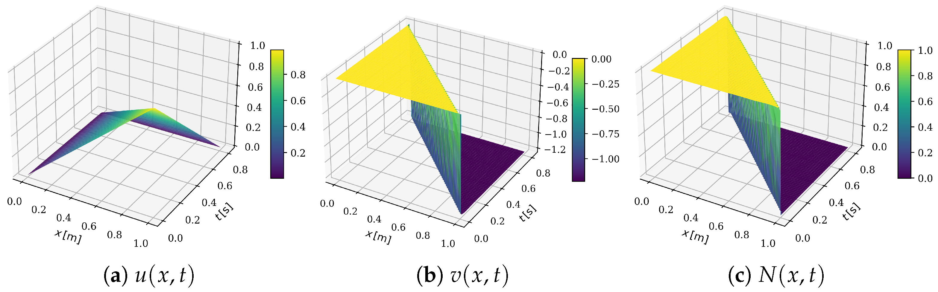
This also has a direct consequence for the differentiated fields. In Case I-A, spatial or temporal differentiation introduces one additional modal factor, so the corresponding series for $\partial u/\partial x$ and $\partial u/\partial t$ decay only as $\mathcal{O}\left({(2n+1)}^{-1}\right)$. In Case I-B, the same differentiation leads to coefficient decay of order $\mathcal{O}\left({(2n+1)}^{-2}\right)$. This explains why the incompatible case is more sensitive near the corner $(L,0)$ and why larger gradients and stronger oscillatory truncation effects may appear there. These two configurations therefore provide complementary verification cases: the first highlights the effect of corner incompatibility, while the second represents a fully compatible and higher-regularity benchmark problem.

Remark on Practical Evaluation and Visualization

The analytical solutions derived above are exact in the form of infinite Fourier-type series. However, the plots shown in this paper are obtained by truncated modal sums, as is customary in practical evaluation. In the computations used for visualization, a sufficiently large but finite number of terms is retained so that the displacement field is accurately represented in the interior of the space–time domain, while the behavior of the differentiated fields remains sensitive to the decay rate of the modal coefficients.

This distinction is particularly important in Case I-A. Since the coefficients decay only as $\mathcal{O}\left({(2n+1)}^{-2}\right)$, the displacement series converges reasonably well, but the convergence of the differentiated series is substantially weaker. As a consequence, the truncated representations of the velocity and especially of the axial force may exhibit visible oscillatory overshoots near the low-regularity region associated with the space-time corner $(L,0)$. These oscillatory features should be interpreted as Gibbs-type ringing of the truncated modal approximation rather than as a failure of the exact analytical representation itself.

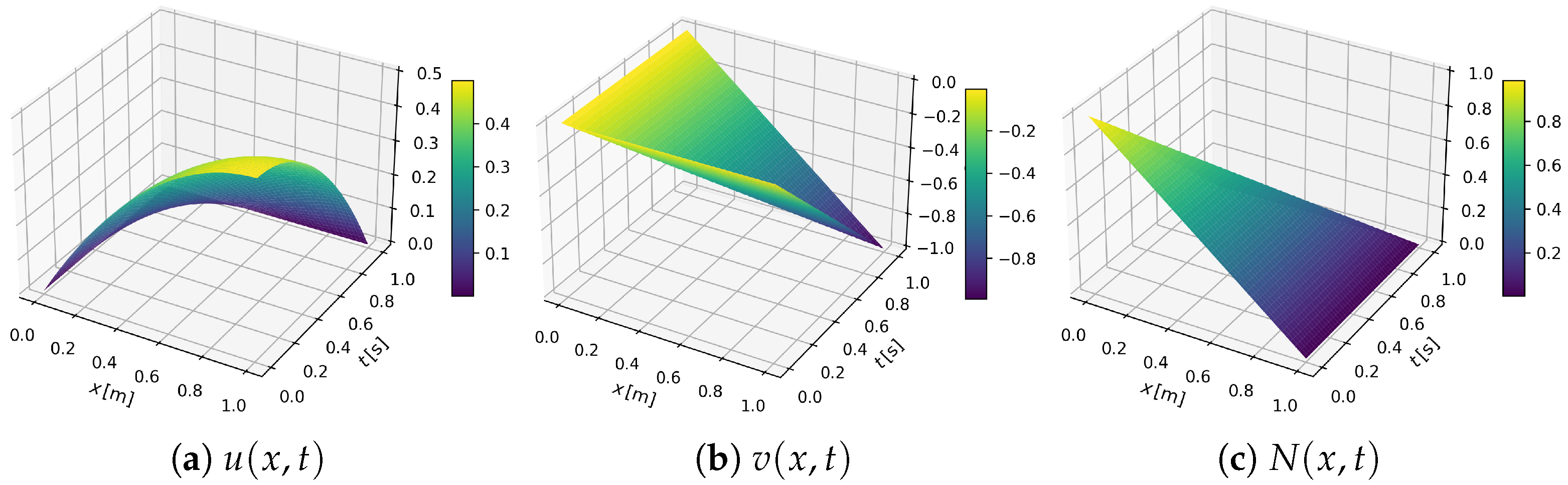
By contrast, in Case I-B the faster coefficient decay $\mathcal{O}\left({(2n+1)}^{-3}\right)$ leads to improved convergence properties for both the displacement and its derivatives. Therefore, the plotted fields in the compatible case are smoother and less prone to oscillatory truncation artifacts. This difference further supports the usefulness of the two benchmark configurations as complementary verification examples for transient numerical solvers.

At the same time, it should be noted that the difference between Case I-A and Case I-B is caused by two mechanisms acting together. The first is the local incompatibility at the space-time corner $(L,0)$, which directly affects the regularity of the differentiated fields near the free end. The second is the higher overall smoothness of the quadratic initial displacement used in Case I-B compared to the linear profile in Case I-A. Therefore, the change in the decay rate of the modal coefficients should be interpreted as the combined effect of corner compatibility and global regularity. A complete separation of these two influences would require additional benchmark families with matched polynomial degree but different compatibility properties. The present paper retains the two simple representative cases because they already provide transparent and practically useful verification configurations.

3.6. Summary of Case I-A and Case I-B

The two benchmark configurations differ both in mathematical structure and physical interpretation. In Case I-A, the linear initial displacement violates the traction-free boundary condition at $x=L$, resulting in corner incompatibility and reduced regularity of the differentiated fields. In contrast, Case I-B satisfies all boundary conditions at $t=0$, leading to faster coefficient decay and higher regularity of the displacement, velocity, and axial force fields. See

Table 1. Comparison of the two initial-value benchmark configurations.

	Case I-A	Case I-B
Initial displacement $u_0\left(x\right)$	$mx$	$x\left(1-{\displaystyle \frac{x}{2L}}\right)$
Compatibility at $x=L$	${\displaystyle \frac{\partial u_0}{\partial x}}\left(L\right)\ne 0$	${\displaystyle \frac{\partial u_0}{\partial x}}\left(L\right)=0$
Corner compatibility	Violated at $(L,0)$	Fully satisfied
Decay of $A_n$	$\mathcal{O}\left({(2n+1)}^{-2}\right)$	$\mathcal{O}\left({(2n+1)}^{-3}\right)$
Physical interpretation	Instantaneous stress adjustment at $x=L$	Smooth stress evolution

.

Finally, if the initial displacement $u_0\left(x\right)$ is a polynomial of degree higher than two and satisfies the boundary conditions at $x=0$ and $x=L$, then the qualitative behavior of the solution is analogous to Case I-B. The increased smoothness of $u_0\left(x\right)$ results in a faster decay of the modal coefficients $A_n$, which in turn ensures improved convergence of the displacement and of its spatial and temporal derivatives. Consequently, both mathematically and physically, the solution exhibits smooth evolution without irregular behavior near the space–time corners.

It should be emphasized that the fields shown in Figure 1 and in Figure 2 represent truncated evaluations of the exact analytical series solution. In the incompatible case, the reduced regularity near the corner $(L,0)$ makes the differentiated fields more sensitive to truncation, and localized oscillatory behavior may therefore appear in the plotted velocity and axial-force distributions.

4. Benchmark Class II: Final-Value Problems

In this section, benchmark configurations are considered in which the displacement field is prescribed at two distinct time instants, namely at $t=0$ and at $t=t_e$. This formulation differs fundamentally from the classical Cauchy-type setting, since the temporal prescription no longer involves the initial velocity but instead imposes displacement constraints at both ends of the time interval.

From a numerical point of view, this class of problems is also of special interest because the two-time displacement prescription is not naturally aligned with standard semi-discrete time-marching formulations, which are typically designed for classical Cauchy-type data. In contrast, formulations that treat space and time in a more symmetric manner—for example, space-time finite element or variational approaches—provide a more natural framework for handling such boundary-value-type temporal constraints. For this reason, the present benchmark class is expected to be particularly relevant for the verification of high-order space-time discretizations. The governing equation remains

$${\displaystyle \frac{{\partial }^{2}u}{\partial t^2}}=c^2{\displaystyle \frac{{\partial }^{2}u}{\partial x^2}},(x,t)\in (0,L)\times (0,t_e),$$

(30)

with mixed spatial boundary conditions

$$\begin{array}{cc}\hfill u(0,t)& =0,\hfill \end{array}$$

(31)

$$\begin{array}{cc}\hfill EA{\displaystyle \frac{\partial u}{\partial x}}(L,t)& =\tilde{F}\left(t\right),\hfill \end{array}$$

(32)

for $t\in (0,t_e)$.

4.1. Formulation of the Benchmark Problem

In the present benchmark configuration, no body force is applied,

$$f(x,t)\equiv 0,$$

and the spatial boundary conditions are

$$\begin{array}{cc}\hfill u(0,t)& =0,\hfill \end{array}$$

(33)

$$\begin{array}{cc}\hfill EA{\displaystyle \frac{\partial u}{\partial x}}(L,t)& =\tilde{F}\left(t\right),\hfill \end{array}$$

(34)

for $t\in (0,t_e)$.

In contrast to the classical initial-value formulation, the displacement is prescribed at two distinct time instants:

$$\begin{array}{cc}\hfill u(x,0)& =0,\hfill \end{array}$$

(35)

$$\begin{array}{cc}\hfill u(x,t_e)& =0.\hfill \end{array}$$

(36)

Thus, the temporal prescription replaces the specification of the initial velocity by a displacement constraint at the final time $t_e$. The right-end traction $\tilde{F}\left(t\right)$ acts as the excitation of the system.

Although this formulation is not a classical Cauchy problem for a hyperbolic equation, the modal construction used below can still be justified in a natural $L^2(0,t_e)$ framework. More precisely, the temporal operator $-{\displaystyle \frac{d^2}{d{t}^2}}$ on $(0,t_e)$ with homogeneous Dirichlet conditions at $t=0$ and $t=t_e$ has the eigenfunctions

$$sin\left({\displaystyle \frac{n\pi t}{t_e}}\right),n=1,2,\dots ,$$

which form a complete orthogonal basis in $L^2(0,t_e)$. Accordingly, the separated representation is understood here as a spectral expansion with respect to this temporal basis. Substitution into the wave equation then yields, mode by mode, the associated spatial boundary-value problems. In this sense, the procedure is not used merely formally, but as the standard spectral decomposition of the one-dimensional Dirichlet Laplacian in time.

Accordingly, the separated representation is used here as a constructive modal benchmark ansatz in the natural $L^2(0,t_e)$ setting, rather than as a complete abstract spectral theory for general final-value problems for hyperbolic equations.

4.2. Separation of Variables

We seek a separated solution of the form

$$u(x,t)=r\left(x\right)w\left(t\right).$$

Substituting into the governing Equation (30) yields

$$r\left(x\right)\ddot{w}\left(t\right)=c^2{r}^{″}\left(x\right)w\left(t\right).$$

Dividing by $c^{2}r\left(x\right)w\left(t\right)$ gives

$${\displaystyle \frac{1}{c^2}}{\displaystyle \frac{\ddot{w}\left(t\right)}{w\left(t\right)}}={\displaystyle \frac{r^{″}\left(x\right)}{r\left(x\right)}}=\lambda ,$$

where $\lambda$ is a separation constant.

The resulting ordinary differential equations are

$$\begin{array}{cc}\hfill \ddot{w}\left(t\right)-c^2\lambda w\left(t\right)& =0,\hfill \end{array}$$

(37)

$$\begin{array}{cc}\hfill r^{″}\left(x\right)-\lambda r\left(x\right)& =0.\hfill \end{array}$$

(38)

4.3. Temporal Eigenvalue Condition

The essential difference from the classical case arises in the temporal Equation (37). The displacement constraints (35) and (36) imply

$$w\left(0\right)=0,w\left(t_e\right)=0.$$

Nontrivial oscillatory solutions require $\lambda <0$. Let

$$\lambda =-{\left({\displaystyle \frac{\omega }{c}}\right)}^2,\omega >0.$$

Then (37) becomes

$$\ddot{w}\left(t\right)+{\omega }^{2}w\left(t\right)=0,$$

whose general solution is

$$w\left(t\right)=Acos\left(\omega t\right)+Bsin\left(\omega t\right).$$

From $w\left(0\right)=0$ it follows that $A=0$, so

$$w\left(t\right)=Bsin\left(\omega t\right).$$

The second temporal condition gives

$$Bsin\left(\omega t_e\right)=0.$$

For nontrivial solutions ($B\ne 0$),

$$sin\left(\omega t_e\right)=0,$$

(39)

which implies

$${\omega }_n={\displaystyle \frac{n\pi }{t_e}},n=1,2,\dots$$

(40)

Thus, in the final-value formulation the eigenvalues are determined by the length of the time interval, rather than by the spatial boundary conditions. The temporal prescription therefore quantizes the admissible frequencies.

4.4. Spatial Modes

Substituting $\lambda =-{\left({\displaystyle \frac{{\omega }_n}{c}}\right)}^2$ into (38) yields

$$r^{″}\left(x\right)+{\displaystyle \frac{{\omega }_n^2}{c^2}}r\left(x\right)=0,$$

with boundary condition $r\left(0\right)=0$.

The general solution is

$$r_n\left(x\right)=a_{n}sin\left({\displaystyle \frac{{\omega }_{n}x}{c}}\right)+b_{n}cos\left({\displaystyle \frac{{\omega }_{n}x}{c}}\right).$$

From $r_n\left(0\right)=0$ it follows that $b_n=0$, so

$$r_n\left(x\right)=a_{n}sin\left({\displaystyle \frac{{\omega }_{n}x}{c}}\right).$$

The spatial structure is therefore governed by the ratio

$${\displaystyle \frac{{\omega }_n}{c}}={\displaystyle \frac{n\pi }{c{t}_e}},$$

which reveals the central parameter of the problem,

$${\displaystyle \frac{L}{c{t}_e}}.$$

This dimensionless ratio determines whether the spatial boundary condition at $x=L$ leads to well-defined modal amplitudes or to singular behavior, as shown in the subsequent subsection.

4.5. Determination of the Modal Coefficients

From the previous subsection, the separated solution takes the form

$$u(x,t)=\sum _{n=1}^{\infty }{d}_{n}sin\left({\displaystyle \frac{n\pi t}{t_e}}\right)sin\left({\displaystyle \frac{n\pi x}{c{t}_e}}\right),$$

(41)

where the temporal frequencies are given by

$${\omega }_n={\displaystyle \frac{n\pi }{t_e}}.$$

The coefficients $b_n$ are determined from the traction boundary condition at $x=L$:

$$EA{\displaystyle \frac{\partial u}{\partial x}}(L,t)=\tilde{F}\left(t\right).$$

Differentiating the series with respect to x yields

$${\displaystyle \frac{\partial u}{\partial x}}(x,t)=\sum _{n=1}^{\infty }{d}_n{\displaystyle \frac{n\pi }{c{t}_e}}sin\left({\displaystyle \frac{n\pi t}{t_e}}\right)cos\left({\displaystyle \frac{n\pi x}{c{t}_e}}\right).$$

Evaluating at $x=L$ gives

$${\displaystyle \frac{\partial u}{\partial x}}(L,t)=\sum _{n=1}^{\infty }{d}_n{\displaystyle \frac{n\pi }{c{t}_e}}cos\left({\displaystyle \frac{n\pi L}{c{t}_e}}\right)sin\left({\displaystyle \frac{n\pi t}{t_e}}\right).$$

Substituting into the boundary condition,

$$EA\sum _{n=1}^{\infty }{d}_n{\displaystyle \frac{n\pi }{c{t}_e}}cos\left({\displaystyle \frac{n\pi L}{c{t}_e}}\right)sin\left({\displaystyle \frac{n\pi t}{t_e}}\right)=\tilde{F}\left(t\right).$$

To determine $d_n$, we multiply both sides by $sin\left({\displaystyle \frac{k\pi t}{t_e}}\right)$ and integrate over $(0,t_e)$. Using the orthogonality relation

$${\int }_0^{t_e}sin\left({\displaystyle \frac{n\pi t}{t_e}}\right)sin\left({\displaystyle \frac{k\pi t}{t_e}}\right)\mathrm{d}t={\displaystyle \frac{t_e}{2}}{\delta }_{nk},$$

(42)

we obtain

$$d_k={\displaystyle \frac{2c}{EAk\pi cos\left(\frac{k\pi L}{c{t}_e}\right)}}{\int }_0^{t_e}\tilde{F}\left(t\right)sin\left({\displaystyle \frac{k\pi t}{t_e}}\right)\mathrm{d}t.$$

(43)

4.6. Singular and Regular Configurations

For each fixed mode k, the coefficient formula (43) is well defined provided that

$$cos\left({\displaystyle \frac{k\pi L}{c{t}_e}}\right)\ne 0.$$

(44)

However, for stability of the coefficient map in the modal setting, a stronger condition is needed, namely that these factors remain uniformly bounded away from zero.

A singular configuration arises if

$$cos\left({\displaystyle \frac{k\pi L}{c{t}_e}}\right)=0,$$

(45)

which is equivalent to

$${\displaystyle \frac{k\pi L}{c{t}_e}}={\displaystyle \frac{\pi }{2}}+l\pi ,k\in \mathbb{N},l\in \mathbb{Z}.$$

(46)

After simplification,

$${\displaystyle \frac{L}{c{t}_e}}={\displaystyle \frac{2l+1}{2k}}.$$

(47)

Thus, singular behavior occurs when the dimensionless ratio ${\displaystyle \frac{L}{c{t}_e}}$ is a rational number of the form ${\displaystyle \frac{2l+1}{2k}}$. In this case, the boundary excitation becomes resonant with the temporally quantized modes, and the coefficient formula (43) loses regularity. Thus, exact singularity occurs when the ratio ${\displaystyle \frac{L}{c{t}_e}}$ satisfies (47). Outside these exact singular ratios, the coefficients are defined mode by mode; however, near-singular parameter values may still lead to strong amplification and poor conditioning.

The singularity condition also admits a direct physical interpretation. The dimensionless ratio $L/\left(c{t}_e\right)$ compares the one-way wave travel time $L/c$ to the prescribed time interval $t_e$. When this ratio satisfies

$${\displaystyle \frac{L}{c{t}_e}}={\displaystyle \frac{2l+1}{2k}},$$

the temporal quantization induced by the two-time displacement prescription becomes commensurate with a spatial mode for which the factor

$$cos\left({\displaystyle \frac{k\pi L}{c{t}_e}}\right)$$

(48)

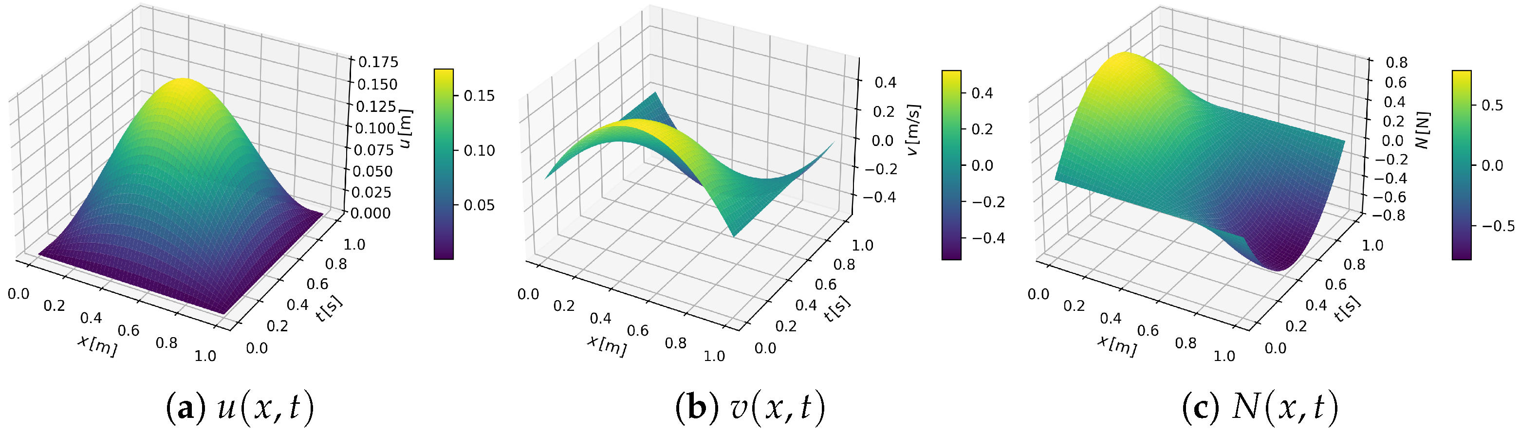
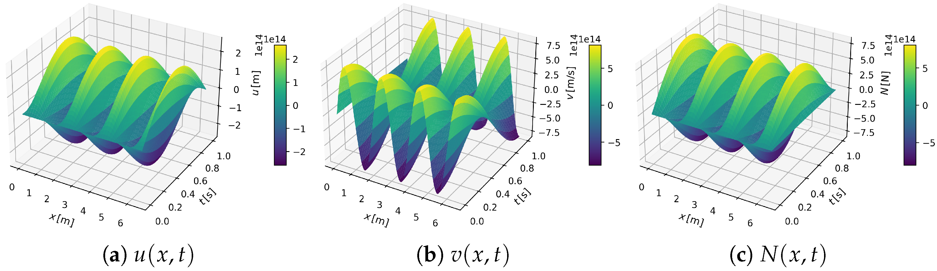
vanishes in the modal coefficient formula. In this situation, the prescribed end traction cannot determine the corresponding modal amplitude in a stable way. Thus, the singular configurations may be interpreted as boundary-driven resonant or critically ill-conditioned cases of the ideal lossless system. From a numerical viewpoint, not only exact singular ratios but also near-singularparameter values are of practical importance. If the ratio $L/\left(c{t}_e\right)$ is close to a value satisfying (47), (48) may become very small for certain modes k, leading to large modal coefficients. (Compare Figure 3 with Figure 4).

This results in strong amplification of selected modes and therefore in ill-conditioned coefficient reconstruction. In numerical computations, such near-singular configurations may manifest as loss of accuracy, sensitivity to discretization errors, and slow convergence of modal or finite element approximations.

Consequently, these near-singular parameter regimes provide particularly demanding test cases for the verification of transient numerical solvers.

4.7. Asymptotic Decay of the Modal Coefficients

From the coefficient formula (43), we have

$$d_k={\displaystyle \frac{2c}{EAk\pi cos\left(\frac{k\pi L}{c{t}_e}\right)}}{\int }_0^{t_e}\tilde{F}\left(t\right)sin\left({\displaystyle \frac{k\pi t}{t_e}}\right)\mathrm{d}t.$$

Assume that the regularity condition (44) holds, so that $cos\left({\displaystyle \frac{k\pi L}{c{t}_e}}\right)$ is bounded away from zero. The asymptotic behavior of $d_k$ is therefore determined by the oscillatory integral

$$I_k:={\int }_0^{t_e}\tilde{F}\left(t\right)sin\left({\displaystyle \frac{k\pi t}{t_e}}\right)\mathrm{d}t.$$

4.7.1. Generic Polynomial Traction

If $\tilde{F}\left(t\right)$ is a polynomial that does not vanish at one or both time endpoints, that is,

$$\tilde{F}\left(0\right)\ne 0\mathrm{or}\tilde{F}\left(t_e\right)\ne 0,$$

then a single integration by parts yields a nonzero boundary term of order $\mathcal{O}\left(k^{-1}\right)$. Consequently,

$$I_k=\mathcal{O}\left({\displaystyle \frac{1}{k}}\right),$$

and therefore

$$d_k=\mathcal{O}\left({\displaystyle \frac{1}{k^2}}\right).$$

(49)

4.7.2. Polynomial Traction Vanishes at Time Endpoints

Suppose now that the traction vanishes at both time endpoints and can be written in the form

$$\tilde{F}\left(t\right)=t^p{(t-t_e)}^q,p,q\in \mathbb{N}.$$

(50)

In this case,

$$\tilde{F}\left(0\right)=0,\tilde{F}\left(t_e\right)=0,$$

so the first boundary term arising from integration by parts vanishes.

Let

$$m=min(p,q).$$

(51)

Then repeated integration by parts shows that the decay rate of the oscillatory integral depends on the parity of m. More precisely,

$$I_k=\mathcal{O}\left({\displaystyle \frac{1}{k^{m+1}}}\right)\mathrm{if}m\mathrm{is}\mathrm{even},$$

(52)

whereas

$$I_k=\mathcal{O}\left({\displaystyle \frac{1}{k^{m+2}}}\right)\mathrm{if}m\mathrm{is}\mathrm{odd}.$$

(53)

Substituting these estimates into (43) yields

$$d_k=\mathcal{O}\left({\displaystyle \frac{1}{k^{m+2}}}\right)\mathrm{if}m\mathrm{is}\mathrm{even},$$

(54)

and

$$d_k=\mathcal{O}\left({\displaystyle \frac{1}{k^{m+3}}}\right)\mathrm{if}m\mathrm{is}\mathrm{odd}.$$

(55)

Therefore, endpoint compatibility of the polynomial excitation improves the decay rate of the modal amplitudes compared to the generic case, and the precise order depends on the vanishing multiplicity at the time endpoints.

4.7.3. Remark on Asymptotic Notation

The estimates derived above are expressed in Big-O notation. We intentionally avoid the use of the asymptotic equivalence symbol ∼, since the coefficients $d_k$ contain oscillatory factors such as ${(-1)}^k$ and $cos\left({\displaystyle \frac{k\pi L}{c{t}_e}}\right)$ in the denominator. Although these terms remain bounded under the regularity condition (44), they do not converge to a fixed nonzero limit as $k\to \infty$.

Therefore, only an upper-order bound of the form

$$d_k=\mathcal{O}\left(k^{-\alpha }\right)$$

can be stated in general, while asymptotic equivalence $d_k\sim C{k}^{-\alpha }$ would require additional assumptions ensuring convergence of the oscillatory prefactors.

4.8. Well-Posedness and Interpretation of Singular Configurations

From a functional point of view, the present two-time formulation is interpreted in a modal Hilbert-space setting. More precisely, the temporal dependence is expanded in the orthogonal basis

$$sin\left({\displaystyle \frac{n\pi t}{t_e}}\right),n=1,2,\dots ,$$

which is complete in $L^2(0,t_e)$ under the homogeneous Dirichlet conditions at $t=0$ and $t=t_e$. The corresponding spatial factors are then determined mode by mode from the wave equation and the mixed boundary conditions.

Accordingly, the notion of well-posedness adopted in this paper is also modal. That is, existence and uniqueness refer to the modal coefficients in the expansion (41) and continuous dependence on the prescribed boundary traction is understood with respect to the boundedness of the coefficient map defined by (43).

In the regular case, the orthogonality relation in time and the explicit coefficient formula define the modal amplitudes uniquely. More precisely, for $\tilde{F}\in L^2(0,t_e)$ and under condition (44), the denominator in the coefficient expression remains bounded away from zero, so the coefficient map from the boundary data to the modal amplitudes is bounded. Consequently, the benchmark problem admits a unique modal solution in the natural $L^2$-based Hilbert-space setting, and the solution depends continuously on the prescribed traction data.

In contrast to the classical Cauchy problem, the temporal prescription (35) and (36) does not define a standard initial-value problem for a hyperbolic equation. However, within the Hilbert space framework, the separated representation (41) is well defined for any boundary excitation $\tilde{F}\left(t\right)\in L^2(0,t_e)$, provided that condition (44) holds. Existence and uniqueness of the modal coefficients follow from the orthogonality relation (42) once the coefficient formula (43) is well-defined mode by mode. Continuous dependence on the boundary data requires the stronger condition that the denominator in (43) remain uniformly bounded away from zero. Therefore, in the present paper, the well-posedness statement is understood only in this regular modal sense. Exact singular ratios given by (47) destroy bounded invertibility, while near-singular parameter values may still lead to substantial conditioning difficulties.

The singular configurations defined by (45)–(47) correspond to vanishing denominators in (43) and therefore to loss of bounded invertibility of the boundary operator. Physically, condition (47) expresses commensurability between the wave travel time $L/c$ and the prescribed time interval $t_e$, leading to boundary-driven resonance. In the ideal lossless model this manifests as strong modal amplification and severe ill-conditioning, which makes such parameter choices particularly suitable for verification of high-order space-time discretizations.

5. Numerical Illustration

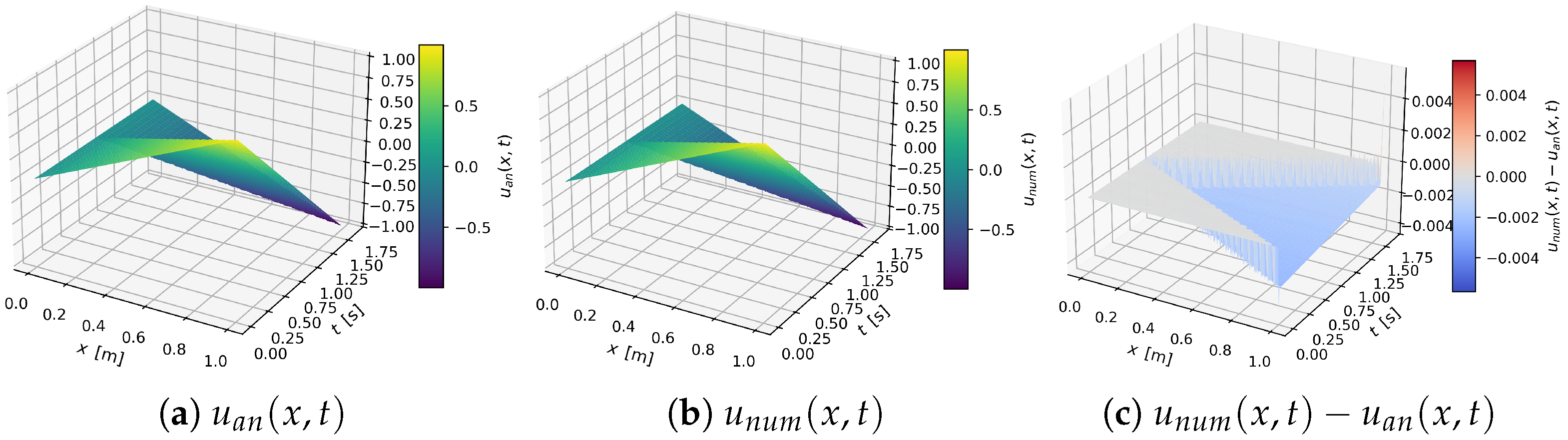
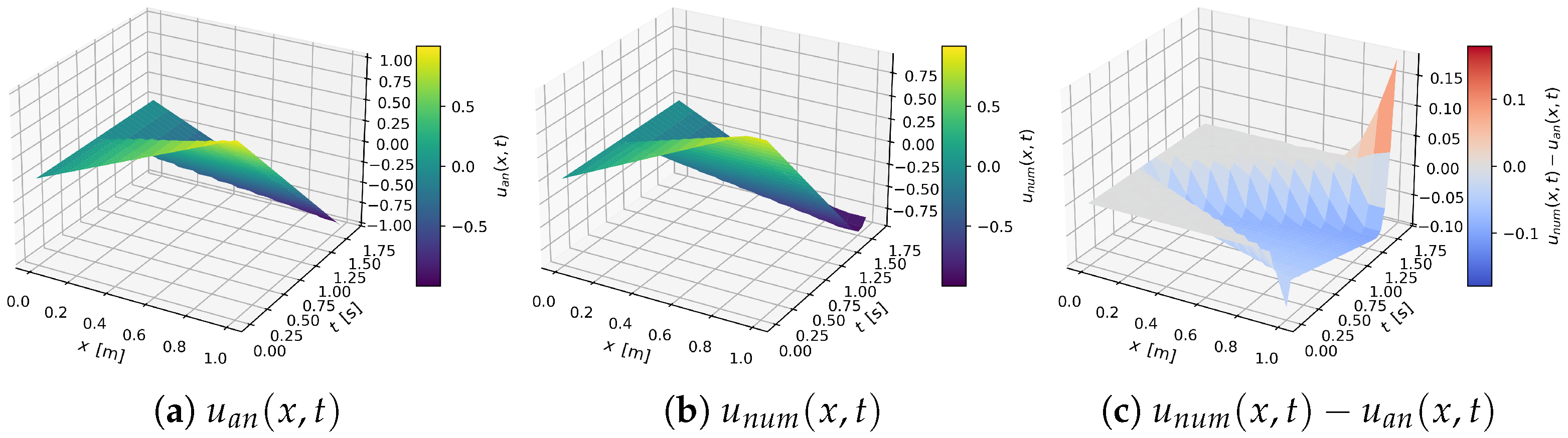
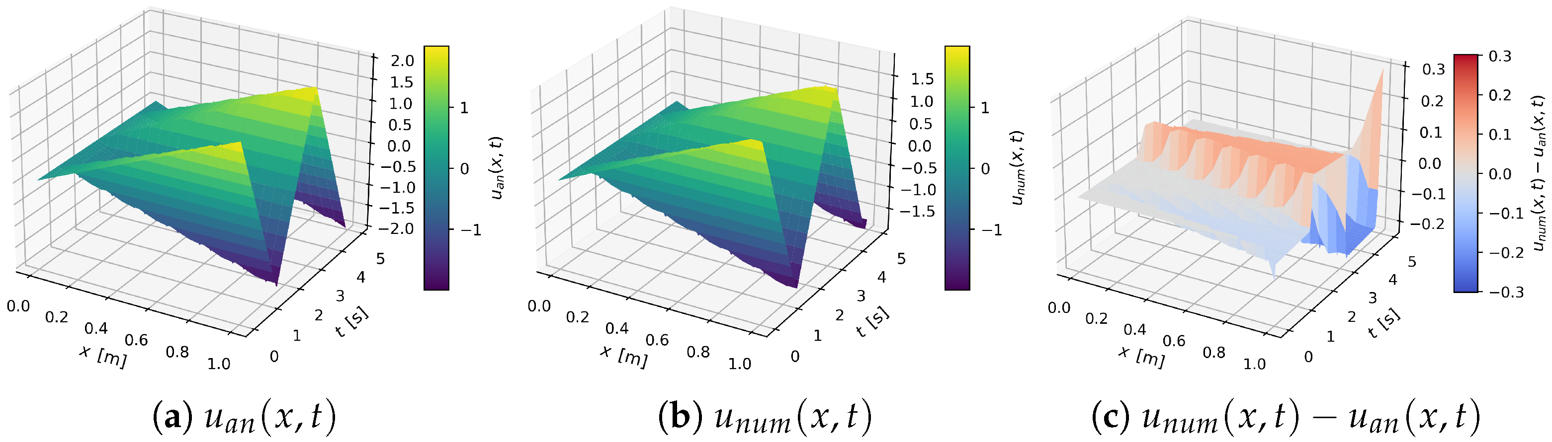
To demonstrate the practical applicability of the proposed benchmark problems, a simple numerical experiment is presented for Case I-A. The purpose of this section is not to introduce a new numerical method but to illustrate how the analytical benchmark reveals characteristic features of standard discretization schemes.

The one-dimensional wave equation was solved using a standard second-order explicit central difference scheme in both space and time. The spatial domain was discretized uniformly with step size $\Delta x$, and the time integration was performed with time step $\Delta t$. The Courant–Friedrichs–Lewy (CFL) condition was satisfied in all cases to ensure stability of the numerical solution.

The mixed boundary conditions were imposed as

$$u(0,t)=0,{\displaystyle \frac{\partial u}{\partial x}}(L,t)=0,$$

while the initial conditions correspond to Case I-A,

$$u(x,0)=mx,{\displaystyle \frac{\partial u}{\partial t}}(x,0)=0.$$

These data are incompatible at the space–time corner $(L,0)$, which results in reduced regularity of the solution.

In order to illustrate the influence of discretization and simulation time, three representative parameter configurations were considered. The results are shown in Figure 5, Figure 6 and Figure 7.

5.1. Fine Discretization

A reference solution was first computed using a fine spatial and temporal discretization (Figure 5). In this case, the numerical solution closely follows the analytical reference over the entire domain. Only minor deviations can be observed near the corner $(L,0)$, where the incompatibility of the data affects the regularity of the solution.

5.2. Coarse Discretization

For a coarse spatial discretization (Figure 6), the numerical solution exhibits noticeable oscillatory artifacts. These oscillations extend further into the domain and are characteristic of the reduced regularity of the exact solution.

5.3. Long-Time Behavior

Finally, the effect of increasing the simulation time is illustrated in Figure 7. The oscillatory patterns originating from the corner incompatibility become more pronounced, demonstrating the long-time impact of such non-compatible data.

These results confirm that the proposed benchmark configurations are well suited for the verification of numerical methods. In particular, they reveal how standard discretization schemes respond to reduced regularity and highlight the importance of compatibility conditions in time-dependent boundary value problems.

6. Conclusions

This paper presented two complementary classes of analytical benchmark problems for the one-dimensional wave equation describing longitudinal vibration of a prismatic elastic rod under mixed (clamped-free) boundary conditions. Closed-form modal solutions were derived in a consistent notation for the displacement field, and the associated velocity and axial force follow directly from the governing relations.

In Benchmark Class I (initial-value problems), two configurations were constructed that differ only in the initial displacement profile. Case I-A intentionally violates the traction-free compatibility condition at the space-time corner $(L,0)$, leading to reduced regularity of the differentiated fields. Case I-B satisfies the boundary compatibility requirements, yielding faster decay of modal coefficients and improved regularity. Together, these two cases provide a clear verification set for assessing how numerical schemes respond to corner incompatibility and convergence limitations. This verification role is also illustrated numerically for Case I-A, where the comparison with a standard finite-difference solution demonstrates that the effect of corner incompatibility becomes increasingly pronounced for coarse discretizations and over longer time intervals.

In Benchmark Class II (final-value problems), the displacement was prescribed at both $t=0$ and $t=t_e$, while the system was excited by a prescribed right-end traction $\tilde{F}\left(t\right)$. The temporal prescription quantizes the admissible frequencies and introduces a fundamentally different spectral structure compared to the classical Cauchy-type formulation. The resulting coefficient expression reveals a nontrivial conditioning mechanism governed by the dimensionless ratio $L/\left(c{t}_e\right)$: singular configurations occur when this ratio takes rational values of the form $(2l+1)/\left(2k\right)$, while regular configurations yield well-defined modal amplitudes.

From the viewpoint of numerical methodology, this benchmark class is especially relevant for formulations that do not rely on standard time marching. Because the displacement is prescribed at both ends of the time interval, the problem is more naturally associated with space-time or variational discretization frameworks than with conventional semi-discrete approaches. The main contribution of the present work is the systematic construction and consistent documentation of analytical benchmark problems for the one-dimensional wave equation under mixed boundary conditions, covering both classical initial-value and non-classical two-time displacement prescriptions.

The results do not introduce new analytical solution techniques for the wave equation; rather, they provide a structured comparison of problem classes that differ in temporal specification and compatibility properties. In particular, the role of space-time corner compatibility in the initial-value formulation and the parameter-dependent spectral structure arising in the final-value formulation are made explicit in a unified framework.

It should be emphasized that the main focus of the present study remains the analytical construction and interpretation of the benchmark families themselves. At the same time, a representative numerical illustration was included for Case I-A in order to demonstrate the practical verification value of the proposed benchmarks. The comparison between analytical and finite-difference solutions shows that fine discretization yields close agreement, whereas coarse meshes and longer simulation intervals amplify the error and make the oscillatory effects associated with corner incompatibility more visible. A broader numerical investigation, including systematic comparisons between semi-discrete and space-time discretization strategies, remains a natural direction for future work.

By identifying the discrete parameter configurations defined by (47) and relating them to loss of bounded invertibility in the modal coefficient expression (43), the paper clarifies the conditioning mechanisms inherent in the two-time formulation. These benchmark configurations are intended to serve as transparent and reproducible reference cases for verification of high-order transient discretization methods.

Several extensions of the present benchmark framework are of clear interest for future research. These include heterogeneous or layered materials, damping effects, nonlinear constitutive behavior, and metamaterial-type structures with dispersive or locally resonant properties. Such generalizations would substantially enrich the range of applicable benchmark problems; however, they would also typically reduce the possibility of obtaining transparent closed-form solutions. For this reason, the present study intentionally focuses on the linear homogeneous one-dimensional setting, where compatibility and spectral conditioning effects can be isolated and analyzed explicitly.

References

1. Korzyuk, V.I.; Naumavets, S.N.; Sevastyuk, V.A. Classical Solution of the Mixed Problem for a One-Dimensional Wave Equation with Second-Order Derivatives at Boundary Conditions. Proc. Natl. Acad. Sci. Belarus Phys. Math. Ser. 2019, 55, 406–412. Available online: https://www.researchgate.net/publication/338550097_Classical_solution_of_the_mixed_problem_for_a_one-dimensional_wave_equation_with_second-order_derivatives_at_boundary_conditions (accessed on 1 April 2026). [CrossRef] [Scilit]
2. Anikonov, D.S.; Konovalova, D.S. Formula for Solving a Mixed Problem for a Hyperbolic Equation. Vladikavkaz Math. J. 2023, 25, 5–13. [Google Scholar] [CrossRef] [Scilit]
3. Khromov, A.P. Behavior of the Formal Solution to a Mixed Problem for the Wave Equation. Comput. Math. Math. Phys. 2016, 56, 243–255. [Google Scholar] [CrossRef] [Scilit]
4. Kornev, V.V.; Khromov, A.P. Resolvent Approach to the Fourier Method in a Mixed Problem for the Wave Equation. Comput. Math. Math. Phys. 2015, 55, 618–627. [Google Scholar] [CrossRef] [Scilit]
5. Fokas, A.S.; Smith, D.A. Evolution PDEs and Augmented Eigenfunctions. Finite Interval. Adv. Differ. Equ. 2016, 21, 735–766. [Google Scholar] [CrossRef] [Scilit]
6. Li, T.; Yu, L. Exact Boundary Controllability for 1-D Quasilinear Wave Equations. Comptes Rendus. Mathématique 2003, 337, 271–276. [Google Scholar] [CrossRef] [Scilit]
7. Batal, A.; Fokas, A.S.; Özsarı, T. Fokas Method for Linear Boundary Value Problems Involving Mixed Spatial Derivatives. Proc. R. Soc. A 2020, 476, 20200076. [Google Scholar] [CrossRef] [Scilit]
8. Graff, K.F. Wave Motion in Elastic Solids; Dover Publications: Mineola, NY, USA, 2012. [Google Scholar]
9. Achenbach, J.D. Wave Propagation in Elastic Solids; North-Holland: Amsterdam, The Netherlands, 1973. [Google Scholar]
10. Courant, R.; Hilbert, D. Methods of Mathematical Physics; Wiley-Interscience: New York, NY, USA, 1962; Volume II. [Google Scholar]
11. Batra, R.C.; Porfiri, M.; Spinello, D. Free and Forced Vibrations of a Segmented Bar by a Meshless Local Petrov–Galerkin (MLPG) Formulation. Comput. Mech. 2008, 41, 473–491. [Google Scholar] [CrossRef] [Scilit]
12. Müller, F.; Schwab, C. Finite Elements with Mesh Refinement for Elastic Wave Propagation in Polygons. Math. Methods Appl. Sci. 2016, 39, 3656–3674. [Google Scholar] [CrossRef] [Scilit]
13. Flyer, N.; Swarztrauber, P.N. The Convergence of Spectral and Finite Difference Methods for Initial-Boundary Value Problems. SIAM J. Sci. Comput. 2002, 23, 1731–1751. [Google Scholar] [CrossRef] [Scilit]
14. Hulbert, G.M.; Hughes, T.J.R. Space-Time Finite Element Methods for Second-Order Hyperbolic Equations. Comput. Methods Appl. Mech. Eng. 1990, 84, 327–348. [Google Scholar] [CrossRef] [Scilit]
15. Fried, I. Finite-Element Analysis of Time-Dependent Phenomena. AIAA J. 1969, 7, 1170–1173. [Google Scholar] [CrossRef] [Scilit] [PubMed]
16. Zienkiewicz, O.C. The Finite Element Method in Engineering Science; McGraw-Hill: London, UK, 1977. [Google Scholar]
17. Zlotnik, A.; Kireeva, O. Practical Error Analysis for the Three-Level Bilinear FEM and Finite-Difference Scheme for the 1D Wave Equation with Non-Smooth Data. Math. Model. Anal. 2018, 23, 359–378. [Google Scholar] [CrossRef] [Scilit]
18. Strikwerda, J.C. Finite Difference Schemes and Partial Differential Equations, 2nd ed.; SIAM: Philadelphia, PA, USA, 2004. [Google Scholar]
19. Friberg, J. Conditionally Stable Difference Approximations for the Wave-Operator. BIT Numer. Math. 1961, 1, 69–86. [Google Scholar] [CrossRef] [Scilit]
20. Carpenter, M.H.; Gottlieb, D.; Abarbanel, S. Time-Stable Boundary Conditions for Finite-Difference Schemes Solving Hyperbolic Systems: Methodology and Application to High-Order Compact Schemes. J. Comput. Phys. 1994, 111, 220–236. [Google Scholar] [CrossRef] [Scilit]
21. Roache, P.J. Verification and Validation in Computational Science and Engineering; Hermosa Publishers: Albuquerque, NM, USA, 1998. [Google Scholar]
22. Zienkiewicz, O.C.; Taylor, R.L.; Zhu, J.Z. The Finite Element Method: Its Basis and Fundamentals, 6th ed.; Butterworth-Heinemann: Oxford, UK, 2005. [Google Scholar]
23. Hornikx, M.; Kaltenbacher, M.; Marburg, S. A Framework for Linear Benchmark Problems in Computational Acoustics. Acta Acust. United Acust. 2014, 101, 811–820. [Google Scholar] [CrossRef] [Scilit]
24. Korzyuk, V.I.; Rudzko, J.V. The Classical Solution of One Problem of an Absolutely Inelastic Impact on a Long Elastic Semi-Infinite Bar. Proc. Natl. Acad. Sci. Belarus Phys. Math. Ser. 2021, 57, 417–427. Available online: https://www.researchgate.net/publication/357356439_The_classical_solution_of_one_problem_of_an_absolutely_inelastic_impact_on_a_long_elastic_semi-infinite_bar (accessed on 1 April 2026). [CrossRef] [Scilit]
25. Korzyuk, V.I.; Rudzko, J.V. The Classical Solution of the Mixed Problem for the One-Dimensional Wave Equation with the Nonsmooth Second Initial Condition. Proc. Natl. Acad. Sci. Belarus Phys. Math. Ser. 2021, 57, 23–32. Available online: https://www.researchgate.net/publication/350615064_The_classical_solution_of_the_mixed_problem_for_the_one-dimensional_wave_equation_with_the_nonsmooth_second_initial_condition (accessed on 1 April 2026). [CrossRef] [Scilit]
26. Khanal, L.; Yang, M.; Pineda, E.J. Hybrid Modeling of Wave Propagation in a 1D Bar: Integrating Peridynamics and Finite Element Methods for Enhanced Dynamic Analysis. Appl. Sci. 2026, 16, 686. [Google Scholar] [CrossRef] [Scilit]
27. Yue, J.; Guo, L.; Guo, P.; Wang, X. Transient Acoustic Wave Propagation Problems in Multilayered Pavement Using a Time Discontinuous Galerkin Finite Element Method. Appl. Sci. 2022, 12, 5438. [Google Scholar] [CrossRef] [Scilit]
28. Liu, S.; Zhou, Z.; Zeng, W. Simulation of Elastic Wave Propagation Based on Meshless Generalized Finite Difference Method with Uniform Random Nodes and Damping Boundary Condition. Appl. Sci. 2023, 13, 1312. [Google Scholar] [CrossRef] [Scilit]
29. Karpik, A.; Cosco, F.; Mundo, D. Dynamic Error Estimation in Higher-Order Finite Elements for Modal and Transient Dynamic Solutions. Designs 2024, 8, 79. [Google Scholar] [CrossRef] [Scilit]
30. Lin, Q.-G. Yet Another Approach to Solutions of One-Dimensional Wave Equations with Inhomogeneous Boundary Conditions. Am. J. Phys. 2022, 90, 31–36. [Google Scholar] [CrossRef] [Scilit]
31. Tóth, B. Multi-field Dual-Mixed Variational Principles Using Non-Symmetric Stress Field in Linear Elastodynamics. J. Elast. 2016, 122, 113–130. [Google Scholar] [CrossRef] [Scilit]
32. Tóth, B. Dual and Mixed Nonsymmetric Stress-Based Variational Formulations for Coupled Thermoelastodynamics with Second Sound Effect. Contin. Mech. Thermodyn. 2018, 30, 319–345. [Google Scholar] [CrossRef] [Scilit]
33. Argyris, J.H.; Scharpf, D.W. Finite Elements in Time and Space. Nucl. Eng. Des. 1969, 10, 456–464. [Google Scholar] [CrossRef] [Scilit]
34. Aharoni, D.; Bar-Yoseph, P. Mixed Finite Element Formulations in the Time Domain for Dynamic Problems. Comput. Mech. 1992, 9, 359–374. [Google Scholar] [CrossRef] [Scilit]
35. Borri, M.; Bottasso, C.; Mantegazza, P. Basic Features of the Time Finite Element Approach for Dynamics. Meccanica 1992, 27, 119–130. [Google Scholar] [CrossRef] [Scilit]
36. Cannarozzi, M.; Mancuso, M. Formulation and Analysis of Variational Methods for Time Integration of Linear Elastodynamics. Comput. Methods Appl. Mech. Eng. 1995, 127, 241–257. [Google Scholar] [CrossRef] [Scilit]
37. Quadrelli, B.M.; Atluri, S.N. Mixed Variational Principles in Space and Time for Elastodynamics Analysis. Acta Mech. 1999, 136, 193–208. [Google Scholar] [CrossRef] [Scilit]
38. Ali, E.J. Modified Treatment of Initial Boundary Value Problems for One Dimensional Heat-Like and Wave-Like Equations Using Variational Iteration Method. Appl. Math. Sci. 2012, 6, 1795–1805. [Google Scholar]
39. Géradin, M. On the Variational Method in the Direct Integration of the Transient Structural Response. J. Sound Vib. 1974, 34, 479–487. [Google Scholar] [CrossRef] [Scilit]
40. Hughes, T.J.R.; Hulbert, G.M. Space-Time Finite Element Methods for Elastodynamics: Formulations and Error Estimates. Comput. Methods Appl. Mech. Eng. 1988, 66, 339–363. [Google Scholar] [CrossRef] [Scilit]
41. Peters, D.A.; Izadpanah, A.P. hp-Version Finite Elements for the Space-Time Domain. Comput. Mech. 1988, 3, 73–88. [Google Scholar] [CrossRef] [Scilit]
42. Ruge, P. Hybrid Time Finite Elements by Discontinuity Control. Comput. Mech. 1996, 17, 392–397. [Google Scholar] [CrossRef]
43. Elishakoff, I.; Tharu, J.K. Sixteen Refined Theories of Longitudinal Vibration of Rods: A Review, from Lord Rayleigh to Modernity. Int. J. Solids Struct. 2026, 331, 113881. [Google Scholar] [CrossRef] [Scilit]
44. Halpern, L. Absorbing Boundary Conditions for the Discretization Schemes of the One-Dimensional Wave Equation. Math. Comput. 1982, 38, 415–429. [Google Scholar] [CrossRef]
45. Hagstrom, T. Radiation Boundary Conditions for the Numerical Simulation of Waves. Acta Numer. 1999, 8, 47–106. [Google Scholar] [CrossRef] [Scilit]
46. Gordin, V.A.; Shemendyuk, A.A. Discrete Transparent Boundary Conditions for the Equation of Rod Transverse Vibrations. Appl. Math. Model. 2020, 85, 220–239. [Google Scholar] [CrossRef] [Scilit]
Figure 1. Displacement, velocity, and normal force distributions in space and time (Case I-A).
Applsci 16 03755 g001
Figure 2. Displacement, velocity, and normal force distributions in space and time (Case I-B).
Applsci 16 03755 g002
Figure 3. Displacement, velocity, and normal force distributions in space and time (Case II regular solution).
Applsci 16 03755 g003
Figure 4. Displacement, velocity, and normal force distributions in space and time (Case II singular solution).
Applsci 16 03755 g004
Figure 5. Comparison of the analytical and numerical solutions for a fine discretization ( L = 1 m , c = 1.5 m / s , t e = 2 L / c , m = 1 , Δ x = 0.005 m , Δ t = 0.004 s , CFL = 0.98 ). Case I-A.
Applsci 16 03755 g005
Figure 6. Comparison of the analytical and numerical solutions for a coarse discretization ( L = 1 m , c = 1.5 m / s , t e = 2 L / c , m = 1 , Δ x = 0.08 m , Δ t = 0.06 s , CFL = 0.92 ). Case I-A.
Applsci 16 03755 g006
Figure 7. Comparison of the analytical and numerical solutions for a moderately coarse discretization over a longer time interval ( L = 1 m , c = 1.5 m / s , t e = 6 L / c , m = 2 , Δ x = 0.05 m , Δ t = 0.04 s , CFL = 0.98 ). Case I-A.
Applsci 16 03755 g007