Article

Horizon Calibration in Highly Deviated Wells and Implications for Velocity-Model Building

1
Hubei Key Laboratory of Complex Shale Oil and Gas Geology and Development in Southern China, Yangtze University, Wuhan 430100, China
2
Research Institute of Exploration and Development, Xinjiang Oilfield Company, PetroChina, Karamay 834000, China
3
No. 1 Oil Production Plant of Xinjiang Oilfield Company, CNPC, Karamay 834000, China
*
Authors to whom correspondence should be addressed.
Appl. Sci. 2026, 16(8), 3628; https://doi.org/10.3390/app16083628
Submission received: 1 February 2026 / Revised: 25 March 2026 / Accepted: 6 April 2026 / Published: 8 April 2026

Abstract

Highly deviated wells commonly exhibit large errors in horizon calibration because the logging path follows an inclined borehole trajectory, whereas post-stack seismic processing effectively treats wave propagation as vertical. This mismatch has received limited attention. Here, we performed horizon calibration and velocity-model building for highly deviated wells drilled in the Mahu Sag, Junggar Basin, and obtained three key findings. First, the assumed vertical travel path in post-stack data is the primary cause of the initial mis-tie for highly deviated wells. Second, calibration in the deviated interval requires a strategy distinct from that of vertical wells and may involve substantial stretching or squeezing of the original logs to achieve a consistent time-depth relationship. Third, the map-view projection of a highly deviated well is essentially linear; relative to vertical wells, it provides denser in situ velocity constraints and, with pseudo-well control, supplies 2D velocity information along the well-trajectory plane, thereby improving velocity-field modeling. Validation against drilling data showed that this workflow improved well ties and refined the velocity model, providing practical guidance for geological well planning and reducing drilling risk.

1. Introduction

Seismic-to-well tie based on synthetic seismograms is a foundational step in structural interpretation and reservoir characterization because it provides the key linkage among seismic observations, geological understanding, and well logs [1,2,3,4]. In recent years, directional drilling—especially highly deviated wells—has been widely adopted in petroleum exploration and development. Such wells enable efficient appraisal of specific targets and can mitigate surface or operational constraints; in some areas, they have become the dominant well type [5,6,7,8,9,10,11,12]. However, generating reliable synthetics for highly deviated wells, quantifying their intrinsic tie errors relative to vertical wells, and exploiting these wells to build accurate velocity models remain practical challenges that must be addressed to support high-resolution exploration and development.
Most industrial workflows generate synthetic seismograms from sonic slowness and density logs using the convolutional model, as implemented in mainstream platforms (e.g., Landmark, GeoEast, Jason) [13,14,15]. For highly deviated wells, the prevailing practice converts measured depth (MD) logs to true vertical depth (TVD), constructs a virtual vertical well from the surface location, generates a 1D synthetic trace using the convolutional model, and then displays this pseudo-seismic trace along the actual well trajectory for matching and horizon calibration against seismic data [16,17]. In addition to the trajectory treatment, multiple factors can control tie quality, including wavelet estimation, borehole/environmental corrections to logs, and seismic polarity determination; these influences and mitigation strategies have been discussed extensively in previous studies [18,19,20,21,22,23,24,25]. Because logging-derived acoustic measurements and seismic data differ strongly in frequency content, velocity estimates from the two domains can diverge. On this basis, some authors have argued that excessive stretching or squeezing of the original logs should be avoided during synthetic generation [26]. This recommendation is generally consistent with vertical wells, where the logging path is broadly aligned with the seismic raypath. In highly deviated wells, however, the inclined borehole trajectory is fundamentally different from the seismic propagation path assumed by post-stack time-domain data, and the resulting mismatch can be much larger, making the role and allowable magnitude of stretching/squeezing in calibration more controversial.
Beyond horizon calibration, highly deviated wells can provide added value for velocity modeling. In map view, a highly deviated well projects approximately as a line and therefore offers denser drilled velocity constraints than a vertical well, potentially improving velocity-field construction. Xiao Dazhi et al. [27] proposed a 3D-model-based method for correcting deviated-well logs and calculating true vertical thickness, but the approach did not explicitly address how to evaluate the accuracy of corrected logs within velocity-model building. After processing steps such as NMO correction and migration, post-stack seismic volumes in the time domain effectively treat wave propagation as vertical. Because the deviated-well logging path differs from this assumed propagation direction, a 1D velocity model derived from a conventional well tie may no longer represent the effective seismic travel velocity for specific depth points along a deviated well. Importantly, the deviated interval provides a series of discrete, reliable time-depth tie points along a 2D line in map view. When these points are incorporated into velocity modeling, velocities above the deviated segment are commonly filled by interpolation or other indirect methods and may carry systematic error. Introducing pseudo-wells can help constrain the velocity information above the deviated section and thereby improve the velocity model, while the set of fixed time-depth points provides a prerequisite for validating the resulting velocity field.
In this study, we use a representative highly deviated well from the Mahu oilfield in China to demonstrate the distinctive characteristics of horizon calibration in highly deviated wells and to quantify how, with pseudo-well constraints, such wells can provide advantages in velocity-field modeling. The proposed workflow is intended to support drilling design in structurally complex areas and during development operations.

2. Data and Methods

To understand why horizon calibration in highly deviated wells can depart systematically from vertical-well practice, it is necessary to separate frequency-related velocity differences from trajectory-related path differences.

2.1. Dispersion and Frequency-Band Mismatch

Atoms, molecules, and rock frameworks exhibit intrinsic vibration (resonance) frequencies. When the frequency of a mechanical wave approaches these intrinsic frequencies, the medium interacts strongly with the wave (absorption and re-radiation), which can modify the propagation speed near that band. As a result, waves of different frequencies can travel at different velocities in the same medium—i.e., dispersion. In practice, sonic logging has an effective frequency of ~5–20 kHz, VSP data ~5–100 Hz, and surface seismic data ~5–70 Hz. Because sonic velocities are measured at much higher frequencies than seismic velocities, dispersion implies that the two velocities are not strictly identical even within the same lithology. Consequently, moderate stretching/squeezing is typically required during synthetic generation and well ties to reconcile time-depth relationships derived from different frequency bands.
Previous studies support that, for many settings, the sonic-to-seismic time-depth relationship can be close. Wang Yanguang et al. [28] constructed velocity information from multi-scale geophysical datasets for Well J41 in the Shengli oilfield and reported that the resulting time-depth relationships were highly similar. Zhang Rong et al. [29] compared sonic-derived interval velocities with seismic interval velocities from 35 wells in the Junggar Basin and obtained an average absolute relative error of 9.7%, i.e.,
|   V sonic V seismic V seismic   | avg = 0 . 097
In post-stack time-domain seismic volumes, the propagation path is effectively treated as zero-offset, vertical (coincident source-receiver). For vertical wells, the logging path and the assumed seismic propagation path are both approximately vertical. Therefore, when generating synthetics for vertical wells, stretching/squeezing primarily compensates for travel-time differences caused by dispersion (i.e., different frequencies sampling slightly different effective velocities in the same medium). A common guideline is that the stretch/squeeze applied during synthetic construction should not exceed ~10%. Jin Ling et al. [26] explicitly stated that excessive stretching or squeezing of the original logs should be avoided during synthetic generation.

2.2. Trajectory-Driven Error in Deviated Wells

For directional/highly deviated wells, the well trajectory is inclined, so the logging path (along the borehole) is no longer consistent with the assumed seismic path (vertical in post-stack time volumes). Relative to vertical wells, the mis-tie in deviated wells thus contains two components over the same vertical depth interval:
  • Dispersion-driven difference between sonic-wave velocity and seismic-wave velocity;
  • Path-driven difference because the sonic measurement samples the formation along an inclined trajectory, whereas the seismic time volume implicitly represents vertical propagation.
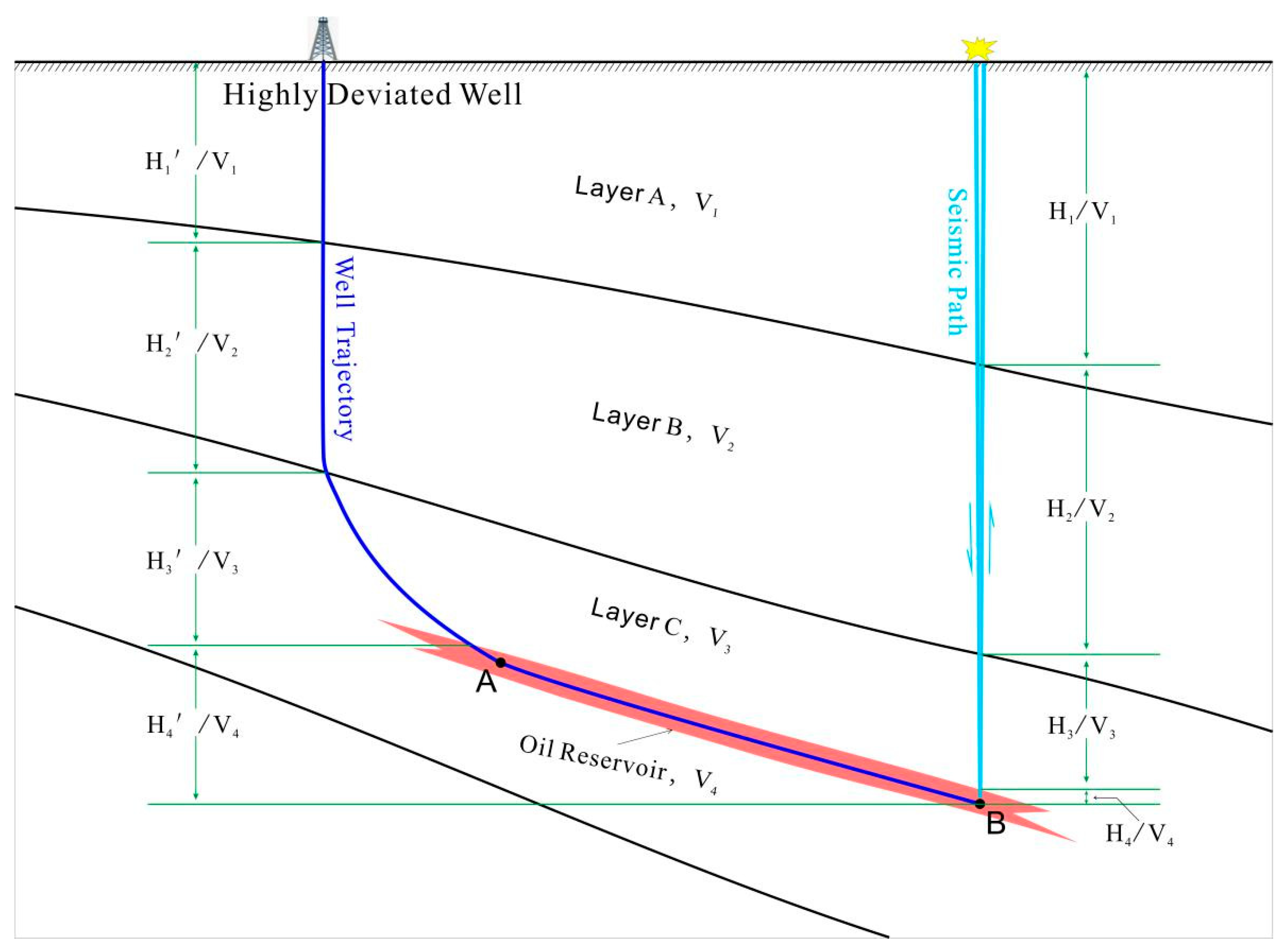
A simple layered geological model (Figure 1) illustrates this effect. For a target point B at true vertical depth H, the vertical depth can be decomposed as
H ( T V D ) = H 1 + H 2 + H 3 + H 4 = H 1 + H 2 + H 3 + H 4
where Hide notes the vertical thickness of layer i, and Hi′ denotes the effective thickness sampled along the deviated well path within the same layer. Although the total TVD is identical, the thickness contribution of each layer differs between the vertical path and the deviated logging path.
If Vi is the interval velocity of layer i, the two-way travel time inferred from the seismic (vertical) path is
T = 2 H 1 V 1 + H 2 V 2 + H 3 V 3 + H 4 V 4
whereas the two-way time implied by the synthetic construction along the deviated sampling path becomes
T = 2 H 1 V 1 + H 2 V 2 + H 3 V 3 + H 4 V 4
Even if the same set of layer velocities is used, T T can arise solely from trajectory-driven differences in Hi versus Hi′. This mechanism explains why highly deviated wells can exhibit a natural, systematic mis-tie that is not fully addressed by vertical-well rules (e.g., strict limits on stretching/squeezing). In other words, stretching/squeezing in deviated intervals is not only compensating for dispersion; it also absorbs part of the geometric mismatch between logging and seismic propagation paths, which becomes more pronounced with increasing deviation and stronger vertical heterogeneity.
Any discrepancy in the velocity (V) can arise from the frequency-band difference between sonic-log and seismic measurements, as expected from dispersion in real rocks. If target B is intersected by a vertical well, then (H = H′) and the only variable is the frequency dependence of velocity. For a directional/highly deviated well, a second variable is introduced because the logging trajectory differs from the seismic propagation path assumed in post-stack time volumes. Therefore, synthetic construction and horizon calibration for directional wells cannot be treated as a straightforward extension of vertical-well practice.
Several workflows have been proposed for improving ties in strongly deviated geometries. For example, Bi Junfeng et al. [30] addressed horizontal wells in which the drilling direction is opposite to the stratigraphic order by reconstructing the sonic slowness and density logs for the lateral section in reverse from the bottom hole, and by generating synthetics using a virtual vertical well anchored at the original bottom-hole location. This approach is effective in specific settings but remains limited; based on the models and examples provided, it is mainly applicable where the strata above the horizontal interval are approximately subhorizontal.
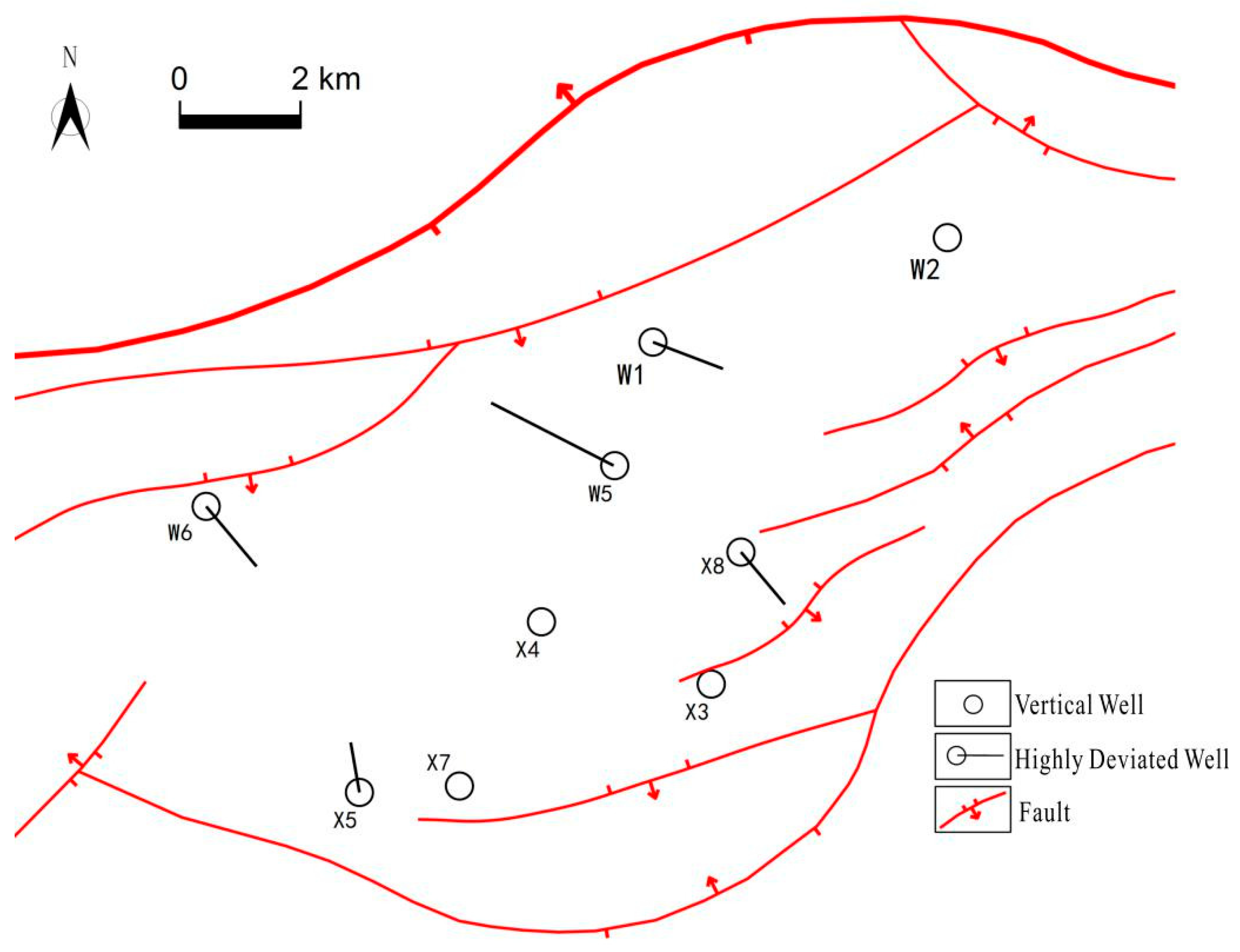
Below, we illustrate the problem and workflow using the highly deviated Well W1 from the Junggar Basin. The Permian shale oil resources in the Wuxia Fault Belt of the western Junggar Basin are abundant, with proven oil reserves exceeding 100 million tons. Among them, five wells have achieved a daily crude oil production of over 100 tons per well. The crude oil is primarily hosted in the Fengcheng Formation, where the reservoir thickness ranges from 10 to 20 m. The formation dip angle of the Fengcheng Formation varies between 5 and 15 degrees, posing significant challenges for the precise development of horizontal wells. Structurally, W1 is located in the Wuxia fault zone of the Western Uplift (Figure 2). The well was drilled to evaluate the hydrocarbon potential of the Permian Fengcheng Formation and to test the effectiveness of producing the target using a high-angle trajectory. W1 reached a measured depth of 5900 m, with a maximum deviation of 79.01°, an azimuth of 108.5°, and a final drilled interval in bottom of the Permian Fengcheng Formation (P1f1).
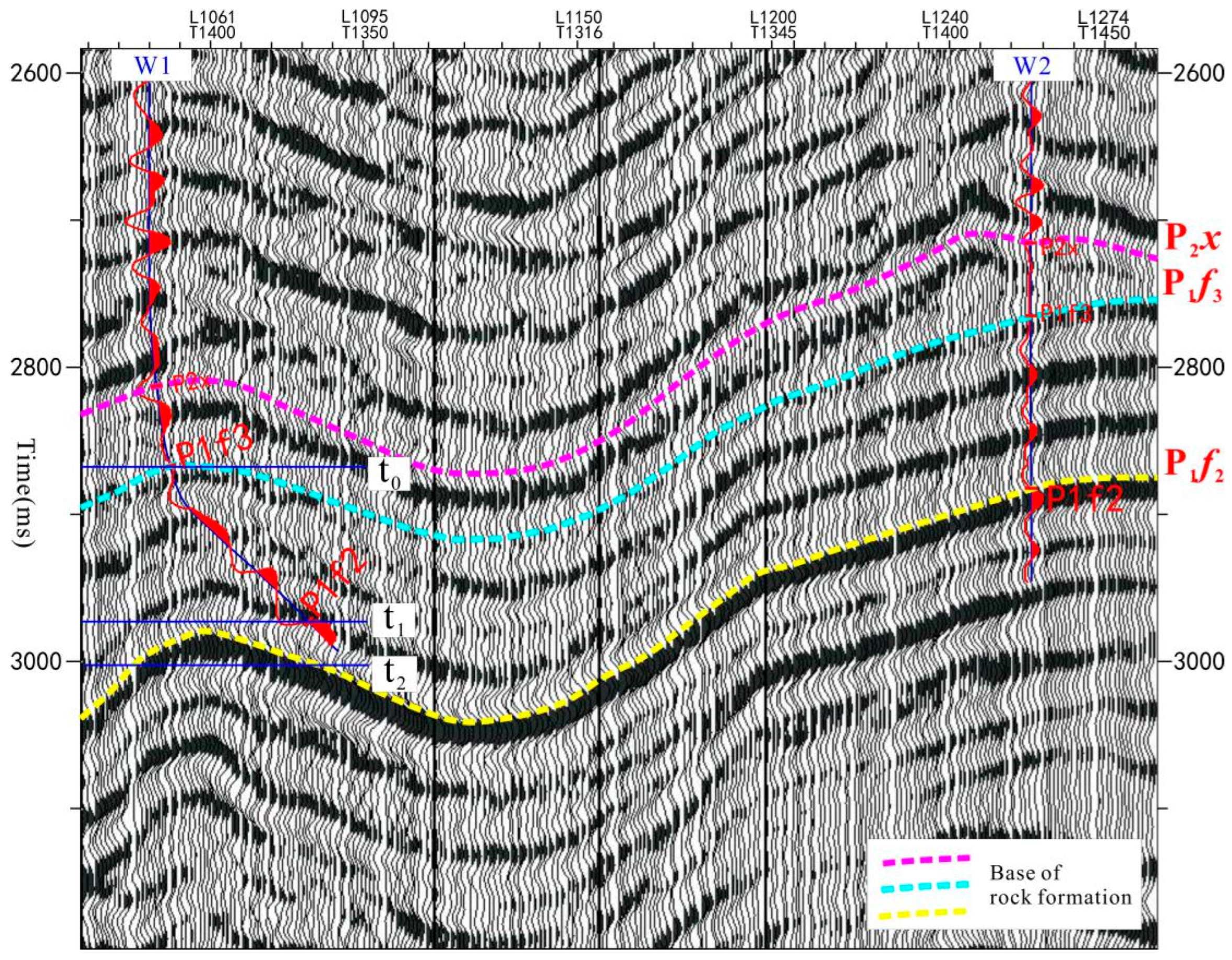
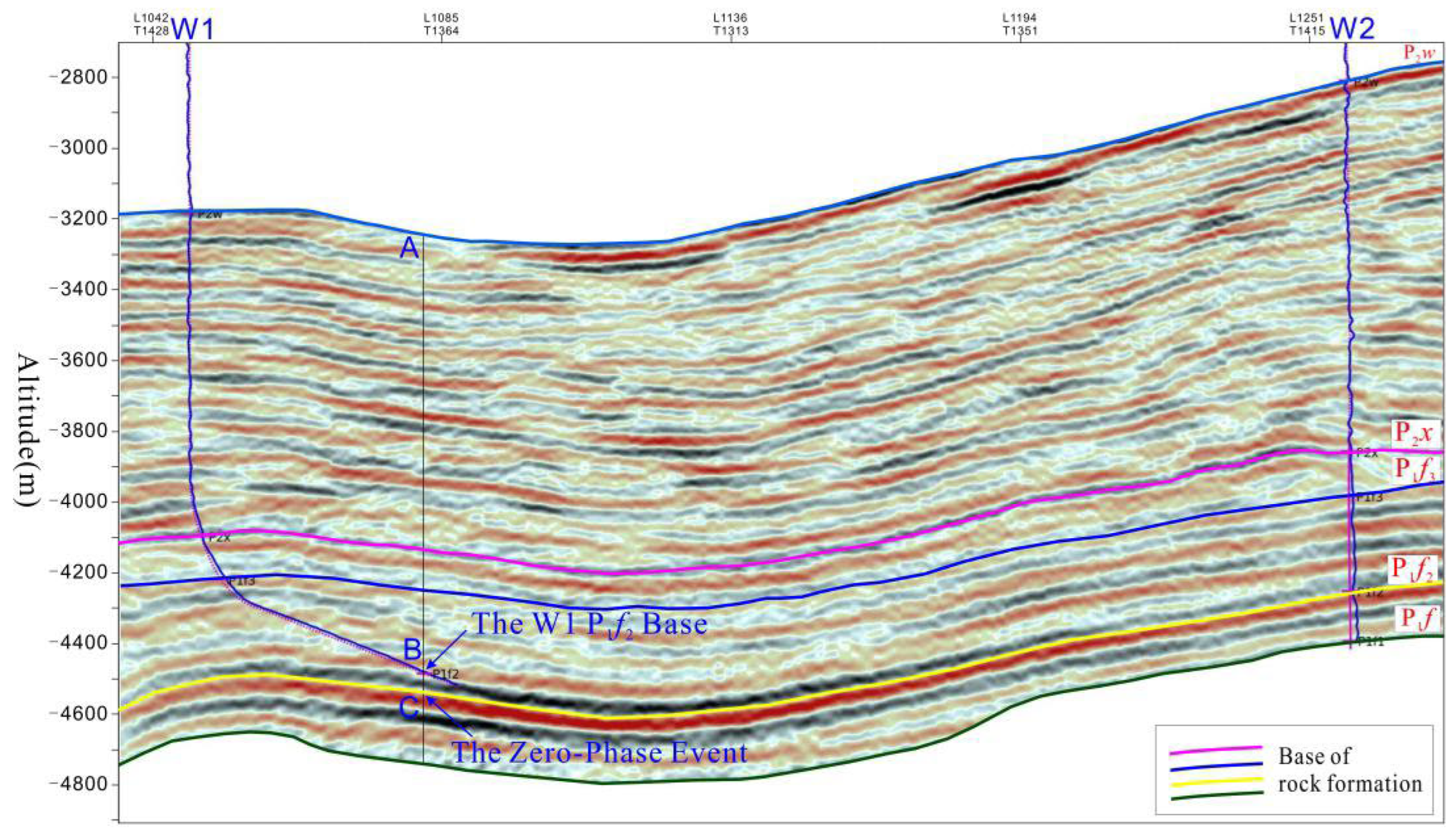
W2 is located east-northeast of W1, and both wells penetrated the base of the Fengcheng Formation (P1f2). Across the study area, the seismic facies at the P1f2 base is laterally stable and consistently occurs at the zero-phase position between a strong trough and a strong peak. We first generated an initial synthetic seismogram for W1 and examined the seismic–geologic interpretation profile connecting W1 and W2 together with the W1 trajectory. Where the lateral displacement of the W1 trajectory was small—i.e., above the base of P1f3 (above t0)—the tie was acceptable. In contrast, below the base of P1f3, the synthetic trace matched the seismic poorly (Figure 3). Specifically, the picked base of P1f2 (at t1) did not fall on the expected zero-phase event (intersection of the yellow horizon and the right side of t2 in Figure 3), and a large stretch was required to move the synthetic to the correct position. Interpreted in terms of the mismatch between the sonic logging path and the seismic propagation path, this behavior indicates that the initial tie for a highly deviated well can be biased, and that substantial stretch/squeeze can be justified during horizon calibration.
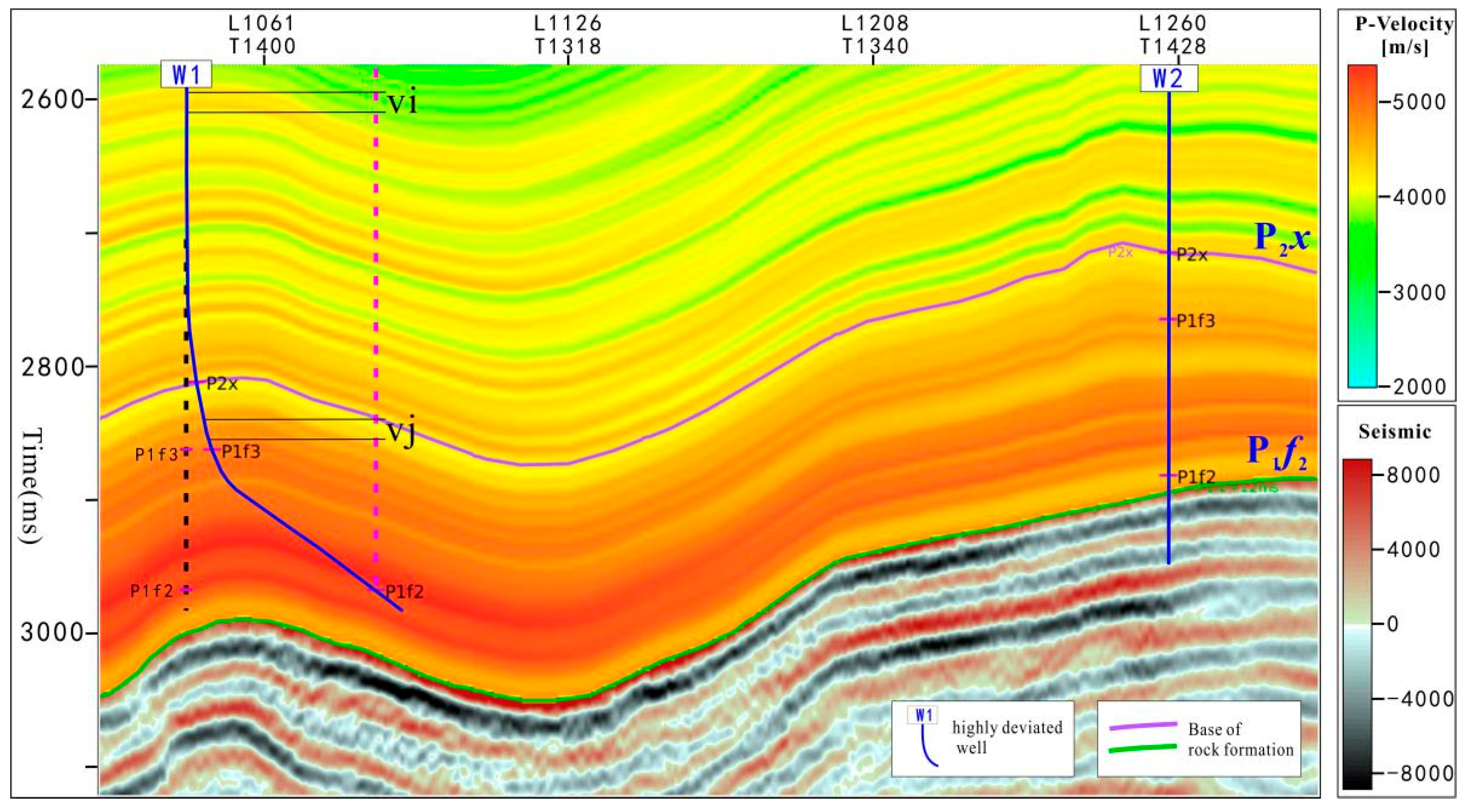
Figure 4 shows the interval-velocity profile along the W1–W2 section. From shallow, younger strata to deeper, older strata, interval velocity increases overall, and the Fengcheng Formation is faster than the overlying Xiazijie Formation (P2x). Following the standard trajectory-handling workflow, we converted measured depth (MD) to true vertical depth (TVD) and constructed a virtual vertical well (black dashed line in Figure 4). We then integrated the interval velocities converted from the sonic slowness to obtain a set of time-depth pairs, and mapped these pairs onto the actual well trajectory to generate an initial seismic-to-well tie for W1 (blue trajectory in Figure 4). However, constrained by the W2 tie and by the regionally consistent seismic signature at the base of P1f2, the initial tie placed the W1 P1f2 base on an incorrect seismic event, with a large mis-tie.
In a time-domain seismic section, the depth associated with a given time sample at a specific trajectory point depends only on the vertically integrated velocities above that point—i.e., the zero-offset (coincident-source-receiver) velocity along the vertical direction. This relationship can be written as
D e p t h ti = v 1 t 1 2 + v 2 t 2 2 + + v n t n 2 ,
where Depthti is the elevation depth corresponding to a time sample on the time-domain section, v1, …, vn are interval velocities, and t1, …, tn are the associated two-way time intervals.
Because the well trajectory is not aligned with the vertical direction, converting a highly deviated well to the TVD domain does not remove the fundamental mismatch between logging-derived velocities and the zero-offset (coincident source-receiver) velocities implied by post-stack time sections. As a result, a synthetic-to-seismic match for highly deviated wells contains an intrinsic, geometry-driven mis-tie.
This error is illustrated using the base of P1f2 in Well W1. The initial synthetic tie placed the P1f2 base at 2973 ms and an elevation depth of −4485.2 m. Over the same time window, the interval velocities above the P1f2 base along the vertical direction (pink dashed line in Figure 4) were systematically lower than those sampled along the deviated well trajectory, as indicated by (Vi) and (Vj) in Figure 4. According to Equation (1), for a given two-way time, lower vertically integrated velocities imply a shallower depth estimate along the vertical path. Therefore, at the W1 trajectory point corresponding to the P1f2 base, (Depth2973, ms) is greater than −4485.2 m, meaning that the true tie position of the P1f2 base should occur below the initial picked position. Using the high-resolution velocity model of the study area for time-depth conversion, we relocated the W1 P1f2 base to 3003 ms on the seismic section (intersection of the yellow horizon with the right side of (t2) in Figure 3). This result demonstrates a substantial discrepancy between the initial and corrected time positions for the P1f2 base, consistent with a large, trajectory-related mis-tie in highly deviated wells.

2.3. Distinctive Features of Horizon Calibration in Highly Deviated Wells and Practical Mitigation

To illustrate the characteristic behavior of horizon calibration in highly deviated wells, we consider the conceptual geological model shown in Figure 1. The true vertical depths (TVDs) in the model were assigned according to the actual geometric scale, and each stratigraphic unit was assigned an interval velocity. For clarity, we initially neglected the frequency-band difference between logging-derived and seismic-derived velocities and focused solely on the trajectory/path effect (Table 1).
For the target point B, the true vertical depth is the same along the vertical and deviated descriptions, i.e.,
H ( T V D ) = H 1 + H 2 + H 3 + H 4 = H 1 + H 2 + H 3 + H 4 = 4000   m
Velocity integration yields the two-way travel time for the seismic (vertical) path and the synthetic (trajectory-sampled) path as
T = 2 H 1 V 1 + H 2 V 2 + H 3 V 3 + H 4 V 4 = 2.386 s , T = 2 H 1 V 1 + H 2 V 2 + H 3 V 3 + H 4 V 4 = 2.273 s .
This simple theoretical model shows that, even when the total TVD is identical, the synthetic trace from a highly deviated well is not expected to align perfectly with the seismic event in time, because the effective thickness contributions (Hi versus Hi′) differ between the vertical propagation assumption and the inclined logging trajectory.
In practice, synthetic seismogram generation follows a standard 1D forward-modeling workflow. Sonic (AC) and density (DEN) logs are used to compute acoustic impedance, from which a reflection-coefficient series r(t) is derived. Convolving r(t) with an estimated seismic wavelet s(t) produces the synthetic trace f(t):
f ( t ) = r ( t ) s ( t ) = 0 S L s ( τ ) r ( t τ ) d τ
where SL is the wavelet length, ∗ denotes convolution, and τ is the integration variable.
Seismic-to-well tie is the process of coupling this 1D synthetic model f(t) to the observed seismic waveform. In our area, the base of P1f2 in vertical wells is consistently expressed as a zero-phase event at the transition between a strong trough and a strong peak (yellow horizon in Figure 3). Therefore, the initial tie for Well W1 required a substantial stretch to place the synthetic event onto the correct regional seismic facies and to maximize waveform coupling along the well trajectory.
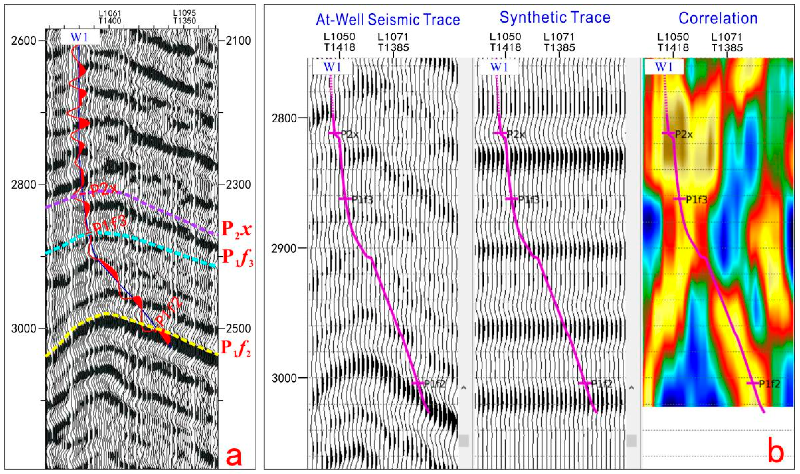
Operationally, we fixed t0 = 2866 ms near the near-vertical part of the well and shifted t1 = 2973 ms downward to t2 = 3003 ms (Figure 3). This corresponds to stretching a 107 ms interval by 30 ms, i.e., a stretch of 28.0%. After stretching, the synthetic trace matched the at-well seismic trace well, and the correlation along the trajectory improved markedly (Figure 5), consistent with the regional seismic facies constraint. The stretch/squeeze amounts applied to other highly deviated wells in the area are summarized in Table 2. These wells consistently displayed considerable stretch/squeeze magnitudes (all considerably large, in contrast to vertical wells).
These results had direct practical implications. The calibrated tie was used in subsequent high-resolution geological modeling, provided a reliable basis for velocity-model refinement in detailed exploration, and supported new-well geological design. Drilling verification indicated that the proposed strategy produced robust horizon calibration for the highly deviated well and effectively reduced drilling risk.

3. Result and Discussion

The fundamental distinction relative to vertical wells is geometric: in vertical wells, the log path is broadly consistent with the (assumed) seismic propagation path, whereas in highly deviated wells, the log path differs from the seismic path, especially in the deviated interval. The farther toward the bottom hole (larger lateral displacement from the wellhead), the less representative the TVD-converted logging velocity becomes for the local seismic travel path. Based on the theoretical analysis and the W1 case study, we draw the following practical conclusions.
  • Horizon picks in highly deviated wells should be guided primarily by regional seismic facies, using waveform coupling between the synthetic and the seismic trace as the quantitative check.
  • Large stretch/squeeze can be justified in the deviated interval to correct for trajectory-driven mis-tie, and the conventional “small stretch only” constraint from vertical-well practice may not apply. This provides a more reliable tie and a stronger data foundation for downstream workflows such as velocity modeling.
Because a highly deviated well follows an inclined trajectory, its map-view projection is essentially a line. Along this trajectory, each measured point provides a deterministic time-depth pair, and thus a dense set of in situ velocity constraints. Compared with vertical wells, highly deviated wells can therefore supply richer drilled velocity information and can be exploited more effectively in velocity-field modeling.
Accurate models are often difficult to obtain in structurally complex areas or where lithology and mineralogy vary rapidly laterally. At well locations, P-wave velocity can be derived reliably from sonic logs and is commonly treated as a “hard” constraint. Between wells, however, velocities are typically populated by interpolation of well-based values or by other indirect approaches, which introduces spatial uncertainty. In a deviated interval, the series of fixed time-depth tie points provides additional geometric control. By introducing pseudo-wells, the velocity information directly above these fixed points can be corrected and better constrained, thereby improving the overall model.
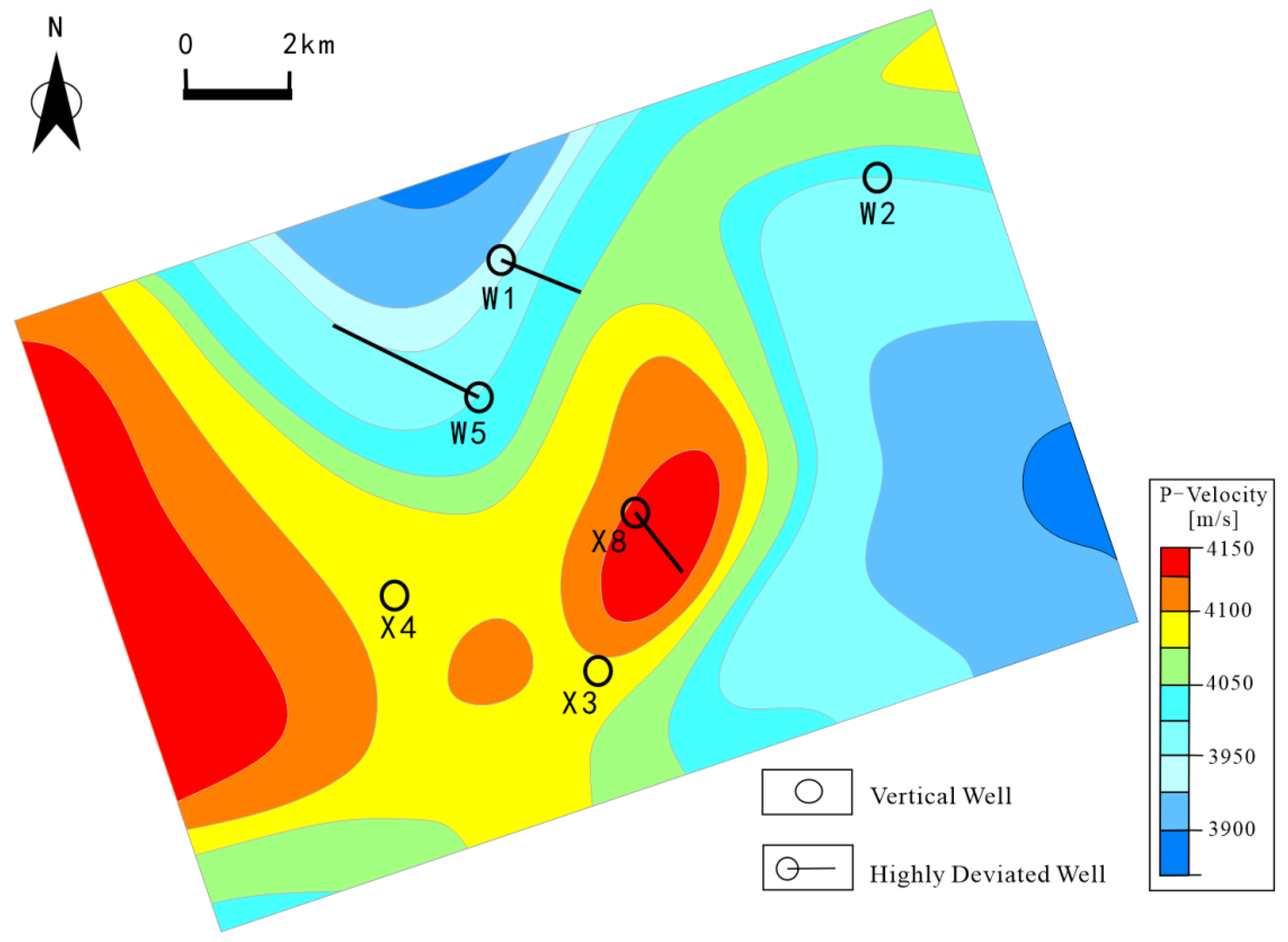
We illustrate this concept using the model around Well W1. The map of interval velocity for the Xiazijie Formation and Fengcheng Formation (Figure 6) shows clear lateral variability. In this model, six wells were used to build the velocity field. At the well locations, the P-wave velocities were taken from measured logs and are thus treated as accurate; the corresponding interval-velocity parameters are listed in Table 3. Across these six wells, the difference between the maximum and minimum velocities is 198.3 m/s, with a mean velocity of 4029.8 m/s, corresponding to a relative spread of ~5%. In contrast, velocities in the interwell region were obtained by interpolation and therefore remain uncertain.
Seismic-to-well tie indicates that, in the W1 area, the base of the Fengcheng Formation (P1f2) should occur at the zero-phase position, marking the transition from a strong trough to a strong peak. We converted the regional time-domain seismic volume to depth using the existing model; however, the converted depth-domain section shows that the W1 P1f2 base does not fall on the zero-phase event identified by the well tie (Figure 7). This mismatch is best explained by lateral variability in interval velocity across the area and by the uncertainty introduced when interwell velocities are populated by interpolation and other indirect methods.
Drilling data provide an independent constraint. At Well W1, the drilled elevation of the P1f2 base is −4486.2 m (point B in Figure 7). After time-depth conversion, the elevation of the same zero-phase tie event is −4536.0 m (point C). From the structural map of the base of the Lower Urho Formation, the elevation directly above the well is −3243.9 m (point A). The true stratigraphic thickness from A to B is therefore 1242.3 m, whereas the converted thickness from A to C is 1292.1 m. The time-depth conversion thus overestimates thickness by 49.8 m (Table 4), indicating that the interval velocity used at this location is lower than the true value (Figure 7). To correct this bias, pseudo-wells need to be introduced to update the P-wave velocity field, while the fixed time-depth points provided by the highly deviated well are used to recover an accurate seismic interval velocity at the well location and, in turn, to improve the model.
We introduced a pseudo-well at the base of P1f2 in the highly deviated Well W1 to correct the local velocity field. The two-way time interval from the base of the Lower Urho Formation to the base of P1f2 is 607.7 ms. Based on the structural map of the Lower Urho Formation, the true stratigraphic thickness between these two horizons is 1242.3 m. Using the two-way travel time from the seismic section, we calculated an effective interval velocity of 4088.5 m/s. In contrast, the existing model assigned an interval velocity of 4252.4 m/s at the same location; the drilling-constrained velocity is therefore 96.14% of the model value.
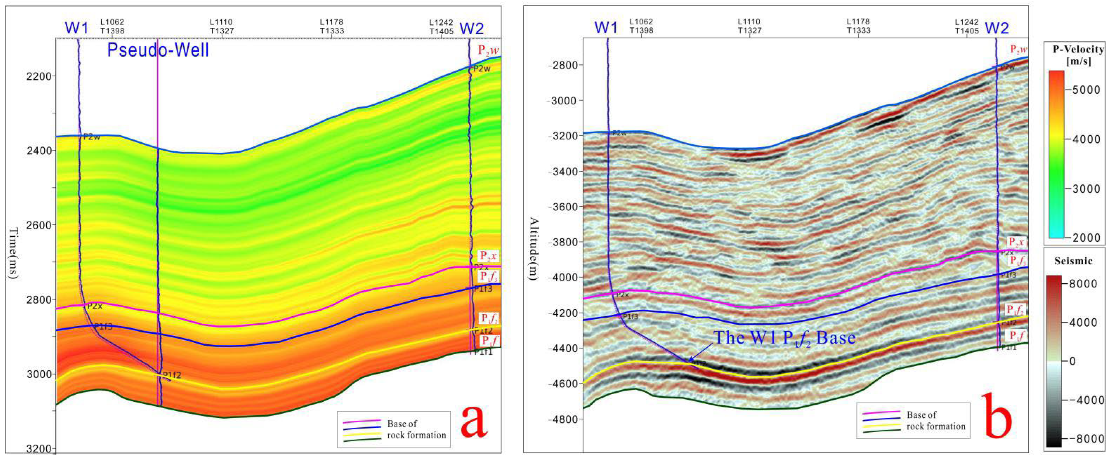
To update the model, we extracted the original velocity function at the pseudo-well from the initial model and scaled the entire curve by 0.9614. The modified pseudo-well velocity function was then incorporated into the velocity-model rebuilding workflow to generate an updated velocity field. In the revised geological model, the base of P1f2 in Well W1 falls at the expected zero-phase position between the trough and peak, consistent with the seismic-to-well tie (Figure 8).
Vertical wells provide 1D velocity constraints along the borehole, whereas highly deviated wells—when combined with pseudo-well constraints—can supply velocity information over a 2D plane aligned with the well trajectory and thus offer a stronger constraint for velocity-field modeling. Because directional wells are affected by trajectory-related mis-tie and can exhibit larger uncertainties in synthetic-to-seismic calibration, they have often been excluded from high-resolution interval-velocity modeling. This practice is suboptimal for the Wuxia fault zone in the Junggar Basin, where the Permian Fengcheng Formation is deeply buried, highly deviated wells are numerous, and several of them serve as key regional control wells. Leveraging these deviated-well constraints in refined velocity modeling is therefore critical for guiding horizontal drilling in the Fengcheng play.
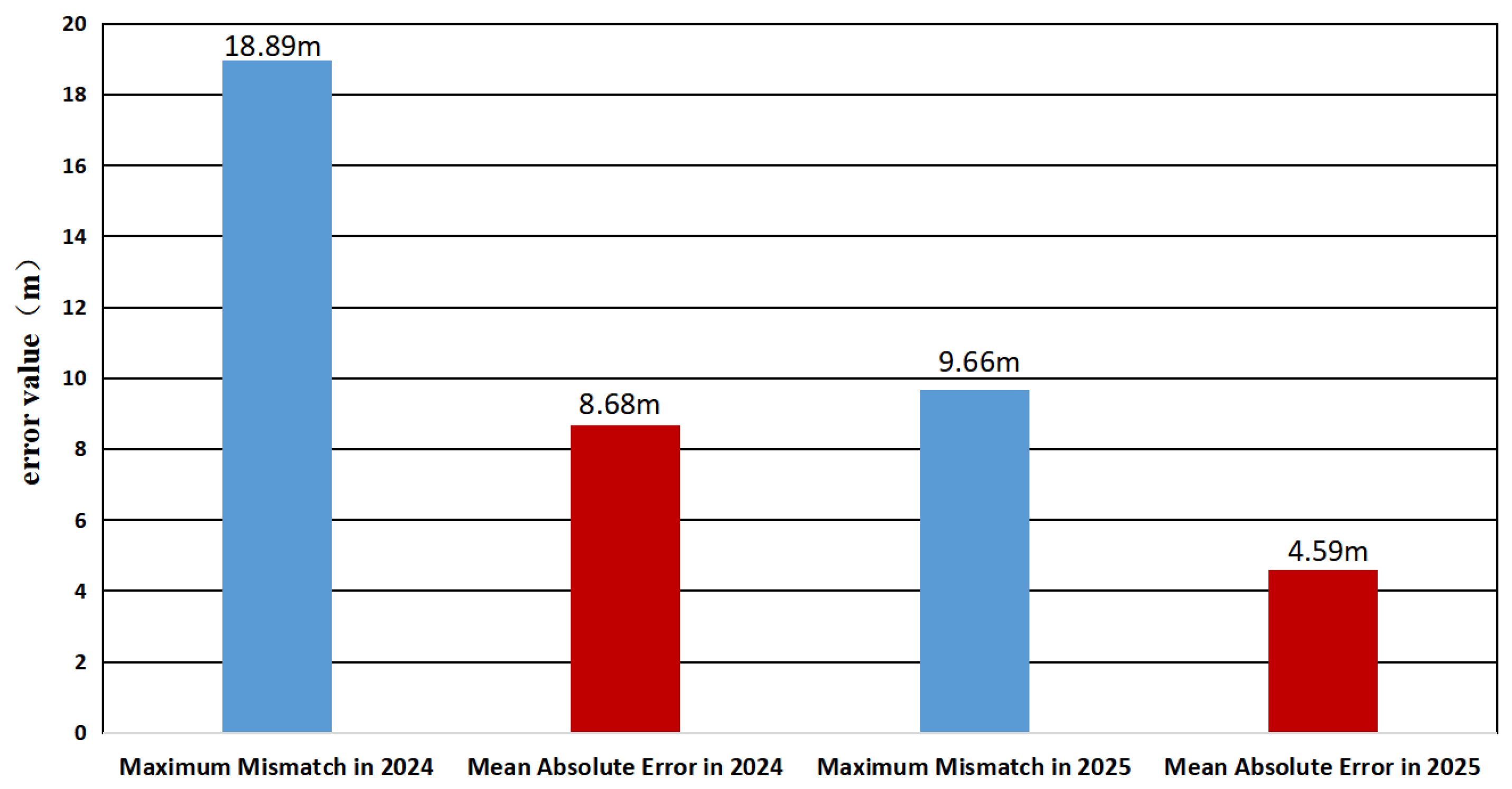
In the Mabei area, the Fengcheng reservoirs occur at ~5000 m depth. For six horizontal wells completed in 2024, the maximum mismatch between the planned and drilled elevations of the A/B targets reached 18.98 m, and the mean absolute error was 8.68 m. In 2025, after pseudo-well constraints were introduced and highly deviated-well data were incorporated into refined velocity modeling—thereby enriching the 2D velocity constraints along well trajectories—the depth-domain model accuracy improved substantially. For the six horizontal wells completed in 2025, the maximum A/B target elevation mismatch decreased to 9.66 m, and the mean absolute error dropped to 4.59 m, markedly improving target prediction and providing more reliable guidance for horizontal drilling (Figure 9).

4. Conclusions

  • Post-stack time-domain seismic volumes obtained after processing steps such as NMO correction and migration effectively assume vertical seismic propagation. In highly deviated wells, the logging path is inclined and therefore differs from this assumed propagation direction. As a result, the 1D velocity model derived from a conventional synthetic tie does not represent the effective seismic travel velocity at specific depth points within the deviated interval, which explains the large bias commonly observed in the initial tie.
  • Workflows developed for vertical-well synthetics are not directly transferable to the deviated interval of highly deviated wells. For these wells, horizon calibration should be guided primarily by regional seismic facies and validated by waveform coupling between synthetic and seismic traces. Accordingly, large stretching/squeezing of the original logs can be warranted, and the conventional “small stretch only” rule of thumb from vertical-well practice may not apply.
  • In velocity-field modeling, vertical wells provide 1D velocity control along depth, whereas highly deviated wells provide a dense set of fixed time-depth points along a near-linear map-view trajectory. With pseudo-well constraints, these data can supply 2D velocity information along the trajectory plane, improve velocity-model accuracy, and produce a more reliable depth-domain model. Drilling results confirmed that the updated depth model provides practical guidance for geological well planning and reduces drilling risk.

Author Contributions

Conceptualization, H.M. and L.Z. (Liping Zhang); methodology, L.Z. (Liping Zhang); software, T.L.; validation, Y.Z., L.Z. (Lei Zhong) and X.C. (Xuan Chen); resources, X.C. (Xiaoxuan Chen); data curation, X.C. (Xiaoxuan Chen); writing—original draft preparation, H.M.; writing—review and editing, L.Z. (Liping Zhang); visualization, T.L.; supervision, Y.Z.; project administration, L.Z. (Liping Zhang); funding acquisition, L.Z. (Liping Zhang). All authors have read and agreed to the published version of the manuscript.

Funding

This research was financially supported by the project “National Science and Technology Major Project (2025ZD1400305)”.

Institutional Review Board Statement

Not applicable.

Informed Consent Statement

Not applicable.

Data Availability Statement

All data and materials are available upon request from the corresponding author. The data are not publicly available due to ongoing research using a part of the data.

Conflicts of Interest

Hailong Ma, Yao Zhao, Lei Zhong and Xiaoxuan Chen were employed by Research Institute of Exploration and Development, Xinjiang Oilfield Company, PetroChina, Karamay 834000, China. Ting Lou was employed by No. 1 Oil Production Plant of Xinjiang Oilfield Company, CNPC, Karamay 834000, China. The remaining authors declare that the research was conducted in the absence of any commercial or financial relationships that could be construed as a potential conflict of interest.

References

  1. Tomassi, A.; De Franco, R.; Trippetta, F. High-resolution synthetic seismic modelling: Elucidating facies heterogeneity in carbonate ramp systems. Pet. Geosci. 2025, 31, 2024–2047. [Google Scholar] [CrossRef] [Scilit]
  2. Ling, Y. The Practice and Exploration of Seismic Data Acquisition, Processing and Interpretation Integration; Petroleum Industry Press: Beijing, China, 2007. [Google Scholar]
  3. Faleide, T.S.; Braathen, A.; Lecomte, I.; Anell, I. Exploring seismic detection and resolution thresholds of fault zones and gas seeps in the shallow subsurface using seismic modelling. Mar. Pet. Geol. 2022, 143, 105776. [Google Scholar] [CrossRef] [Scilit]
  4. Noureddine, M.A.; De Martin, F.; El Meouche, R.; Sammuneh, M.A.; Ababsa, F.; Beaufils, M. Neural Network-Based Metamodel of synthetic seismograms: Application for uncertainty quantification. Eng. Appl. Artif. Intell. 2025, 151, 110613. [Google Scholar] [CrossRef] [Scilit]
  5. Eivazi, R. A novel analytical approach to design horizontal well completion using ICDs to eliminate heel-toe effect. Sci. Rep. 2025, 15, 11094. [Google Scholar] [CrossRef] [Scilit]
  6. Xiao, H.M.; Luo, Y.C.; Zhao, X.L.; Zhang, H.Q.; Liu, X.W. Factors Influencing Productivity of Horizontal Wells with CO2 Inter-Fracture Flooding. Xinjiang Pet. Geol. 2022, 43, 479–483. [Google Scholar]
  7. Zhang, J.; Hu, D.D.; Qin, J.H.; Wang, Y.W.; Tang, H.Y. Optimization of Key Fracturing Parameters for Profitable Development of Horizontal Wells in Mahu Conglomerate Reservoirs. Xinjiang Pet. Geol. 2023, 44, 184–194. [Google Scholar]
  8. Yushchenko, T.; Demin, E.V.; Khabibullin, R.A.; Sorokin, K.S.; Khachaturyan, M.V.; Baykov, I.V.; Gatin, R.I. Case Studies and Operation Features of Long Horizontal Wells in Bazhenov Formation. SPE Prod. Oper. 2023, 38, 185–199. [Google Scholar] [CrossRef] [Scilit]
  9. Al-Rashidi, H.; Hussein, M.R.; Erhamah, A.; Malik, S.; Al-Hajri, A.; Salehi, N.; Rossi, G.O.; Zaitoun, A.; Almeida, D. Mitigating Water Production from High Viscosity Oil Wells in Unconsolidated Sandstone Formations. SPE Prod. Oper. 2022, 37, 762–766. [Google Scholar] [CrossRef] [Scilit]
  10. Zheng, J.; Fu, Y.Q.; Chen, M.; Jing, C.; Zhang, J.; Zhou, H.; Zhang, J.H. Application of Vertical P-Wave Slownesses in Porosity Evaluation of Shale Gas Reservoirs in Highly Deviated or Horizontal Wells. Xinjiang Pet. Geol. 2021, 42, 598–604. [Google Scholar]
  11. Ramirez Palacio, G.J.; Almario, F.; Chacon, A.C.; Rojas, E.M.; Hernandez, N.J.; Valencia, M. Production Profiles Recorded Using Fiber-Optic Technology in Wells with Electrical Submersible Pump Lift System. SPE Prod. Oper. 2023, 38, 746–763. [Google Scholar] [CrossRef] [Scilit]
  12. Singh, U.; Pathan, R.; Joshi, A.D.; Cavé, A.; Fouchard, C.; Baume, A. Accelerated Design of Sidetrack and Deepening Well Trajectories. SPE J. 2023, 29, 1862–1872. [Google Scholar] [CrossRef] [Scilit]
  13. Fang, X.D. A grouped calibration method of synthetic seismograph with complex geology: A case study of Gunan-209 area, Shengli oilfield. China Offshore Oil Gas 2006, 18, 313–315. [Google Scholar]
  14. Yuan, L.H.; Liu, H.; Li, J.H. Application of Well Seismic Joint Fine Calibration Technology in Stratigraphic Correlation of Hailar Basin. J. Oil Gas Technol. 2012, 34, 63–67. [Google Scholar]
  15. Sun, Z.T.; Meng, X.J.; Shen, G.Q.; Niu, X.M.; Ji, Y.X.; Wang, Y.M. The technology of making high-precision synthetic seismogram. Oil Geophys. Prospect. 2002, 37, 640–643. [Google Scholar]
  16. Zhang, Y.H.; Li, G.L. Deviated Well Horizon Calibration Technology and Its Application. Geophys. Prospect. Pet. 1999, 38, 121–126. [Google Scholar]
  17. Zhang, X.K.; Zhou, Y.X.; Liu, B. Method for making an inclined well synthetic seismogram. Oil Geophys. Prospect. 2000, 35, 774–778. [Google Scholar]
  18. AlGharbi, W.M.; Bell, R.E.; John, C.M. SRT-AI: Identifying seismic reflection terminations using deep learning. Appl. Comput. Geosci. 2025, 27, 100271. [Google Scholar] [CrossRef] [Scilit]
  19. Sun, Z.C.; Gu, Z.G.; Li, J.; Yang, B. Correction of well logs in the case of severe borehole enlargement. Xinjiang Pet. Geol. 2006, 27, 559–561. [Google Scholar]
  20. Zhang, J.-H.; Zhang, B.-B.; Zhang, Z.-J.; Liang, H.-X.; Ge, D.-M. Low-frequency data analysis and expansion. Appl. Geophys. 2015, 12, 212–220. [Google Scholar] [CrossRef] [Scilit]
  21. Song, J.G.; Li, H.; Liu, L.; Liu, L.Y. Quality control methods of synthetic seismograms. Prog. Geophys. 2009, 24, 176–182. [Google Scholar]
  22. Galiana-Merino, J.J.; Rosa-Herranz, J.L.; Rosa-Cintas, S.; Martinez-Espla, J.J. Seismic Wave Tool: Continuous and discrete wavelet analysis and filtering for multichannel seismic data. Comput. Phys. Commun. 2013, 184, 162–171. [Google Scholar] [CrossRef] [Scilit]
  23. Dahlin, A.; Lecomte, I.; Senger, K.; Smyrak-Sikora, A.; Braathen, A.; Stemmerik, L. Analysing lithological complexity in outcrop-scale seismic models of interbedded siliciclastics and carbonates from Svalbard. Mar. Pet. Geol. 2025, 181, 107494. [Google Scholar] [CrossRef] [Scilit]
  24. Mu, Q.; Li, G.; Zhang, W.; Chi, R. Effectiveness evaluation of tight sandstone reservoirs based on NMR logging. Xinjiang Pet. Geol. 2025, 46, 121–126. [Google Scholar]
  25. Tschannen, V.; Ghanim, A.; Ettrich, N. Partial automation of the seismic to well tie with deep learning and Bayesian optimization. Comput. Geosci. 2022, 164, 105120. [Google Scholar] [CrossRef] [Scilit]
  26. Jin, L.; Su, G.Z.; Liu, G.L.; Zhu, P.Y.; Li, L.; Hu, Y.P. The influencing factors and countermeasures of synthetic seismic record production. Geophys. Prospect. Pet. 2004, 43, 267–271. [Google Scholar]
  27. Xiao, D.Z.; Luo, Y.H.; Zeng, X.H.; Fang, X.Y.; Chen, K.; Huan, J.L. Inclined Well Logging Curve Correction and True Vertical Thickness Calculation Method Based on 3D Modeling. Chin. J. Eng. Geophys. 2023, 20, 281–289. [Google Scholar]
  28. Wang, Y.G.; Han, W.G.; Liu, H.J. Analysis and matching of multi-scale geophysical data. Oil Geophys. Prospect. 2008, 43, 333–339. [Google Scholar]
  29. Zhang, R.; Xu, Q.Z.; Parhat; Wang, H.Y.; Wei, J.L. Discussion on Improving the Precision of Formation Pressure Prediction: The Relationship between Sonic Logging Formation Velocity and Seismic Formation Velocity. J. Oil Gas Technol. 2010, 32, 274–276. [Google Scholar]
  30. Bi, J.F.; Cai, J.H. A method for making and calibrating synthetic records of horizontal wells: A case study on Well Zhuang 202-Ping 1 in the Zhanhua sag. China Pet. Explor. 2018, 23, 88–93. [Google Scholar]
Figure 1. Schematic illustration of travel-time to a specific depth point during seismic-to-well tie for a directional well.
Applsci 16 03628 g001
Figure 2. Structural location map of Well W1.
Applsci 16 03628 g002
Figure 3. Seismic–geological interpretation profile along the well tie line of W1–W2 wells.
Applsci 16 03628 g003
Figure 4. Interval velocity profile along the W1–W2 wells. (The vertical axis represents two-way travel time (TWT), and the horizontal axis corresponds to the seismic section along the W1–W2 wells. The velocity profile, displayed in a color scale ranging from light blue to green to yellow to red, is overlain on the seismic section.)
Applsci 16 03628 g004
Figure 5. Well-tie results after applying a 28.0% local stretch to the synthetic seismogram. (a) Seismic section through Well W1. (b) Comparison of the at-well seismic trace, synthetic trace, and their correlation.
Applsci 16 03628 g005
Figure 6. Planar Velocity Map of the Xiazijie Formation and Fengcheng Formation in the W1 Well Area.
Applsci 16 03628 g006
Figure 7. Depth-Domain Seismic Profile After Time-Depth Conversion Along the W1–W2 Wells.
Applsci 16 03628 g007
Figure 8. Updated velocity-model sections and time-depth conversion results using a pseudo-well constraint. (a) Updated interval-velocity section along the W1-pseudo-well-W2 profile. (b) Updated depth-domain seismic section along the W1–W2 profile.
Applsci 16 03628 g008
Figure 9. Comparison of predicted target accuracy for horizontal wells drilled in 2024 and 2025.
Applsci 16 03628 g009
Table 1. Vertical depth and interval velocity parameters of the geological model encountered by directional drilling.
Formation TVD (m)Seismic TVD (m)Interval Velocity (m/s)
H1′: 974H1: 1633V1:3000
H2′: 1240H2: 1560V2:3500
H3′: 930H3: 727V3:4000
H4′: 856H4: 80V4:3800
Table 2. Statistics on the stretch/squeeze of synthetic seismograms for highly deviated wells drilled in the Permian formations within the Wuxia Fault Belt of the western Junggar Basin.
Well LocationW5W6X5X8
stretch/squeeze (%)20242927
Table 3. Interval-velocity parameters for the Xiazijie Formation and Fengcheng Formation in the W1 area.
Well LocationW1W2W5X3X4X8
Interval velocity (m/s)3935.33965.43971.84092.44068.54133.6
Interval-velocity deviation from the mean (m/s)−92.5−63.4−58.061.636.7100.8
Table 4. Statistical table of relevant parameters and errors between the actual and initial conversion models for Well W1.
Elevation of the Base of P1f2 (m)Stratigraphic Thickness (m)Interval Velocity (m/s)
Initial time-depth conversion model−4536.01292.14252.4
Measured at Well W1−4486.21242.34088.5
Error−49.849.8163.9
Disclaimer/Publisher’s Note: The statements, opinions and data contained in all publications are solely those of the individual author(s) and contributor(s) and not of MDPI and/or the editor(s). MDPI and/or the editor(s) disclaim responsibility for any injury to people or property resulting from any ideas, methods, instructions or products referred to in the content.