Parameterized Clearance Cost-Shaping for Any-Angle Planning: Quantifying Safety–Efficiency Trade-Offs on Grid Maps

Abstract

This study examines a cost-shaping method that considers distance information to obstacles in a line-of-sight (LOS) any-angle path-planning approach on grid-based maps. In the proposed approach, the safety distance to obstacles is added to the cost in a controlled manner via a single adjustable and interpretable parameter; thus, the balance between safety and efficiency becomes practically adjustable. Node selection in the planning process is performed while maintaining the classical search rule; the additional penalty related to the safety distance is only included in the transit cost. This design strengthens consistency between method definition and implementation and eliminates the risk of the same safety term being considered multiple times. The experimental evaluation was conducted on a three-by-three scenario set encompassing map type and difficulty level dimensions. Starting and ending points were selected in a layered and matched manner as easy/medium/difficult; the safety parameter was scanned at different values, following a repeatable protocol under all conditions. Outputs were evaluated using efficiency metrics such as path length and number of turns, as well as minimum safety distance, safety distance violation rate, and a curvature indicator representing the smoothness of the path geometry. In addition, practical costs such as planning time, an expanded number of nodes, and memory footprint were reported. The results show that exposure to low safety distance zones decreases and the path geometry becomes more regular with increasing safety parameters. Furthermore, it was observed that the success rate increased in pooled analyses while memory usage remained constant; paired statistical tests and effect size measurements confirmed that the improvements were strong and consistent. These findings reveal that safety distance-sensitive cost-shaping offers a lean control mechanism that enhances safety and maintains practical applicability within line-of-sight-based any-angle planning.

1. Introduction

In the field of autonomous robotics, path planning remains one of the most critical problems. The main goal is to determine a collision-free and optimal path from a starting point to a destination in a fully or partially known environment. In this context, grid-based search algorithms such as A* and D* have long been considered reliable solutions due to their comprehensiveness and optimality assurances in discrete space [1,2,3,4]. However, since these classical methods often restrict movement to grid connections, such as 4- or 8-neighborhood, they can produce “unnatural” zigzagging and excessively discretized paths in practice. As a result, path length, travel time, and energy consumption in real-world scenarios can increase unnecessarily [5,6,7].

To overcome these limitations, researchers have developed numerous any-angle path-planning approaches that relax the grid alignment constraint and allow movement in different directions while preserving the fundamental principles of heuristic search. This family of methods includes Theta* [8], Lazy Theta* [9], Field D* [10], Block A* [11], and ANYA [12], each offering a different balance in terms of optimality, smoothness, and runtime complexity. However, since these methods are implemented in different ways in practice and evaluated with different protocols, it is often difficult to directly compare their results under the same conditions.

In real-world robot navigation, the planner must reduce not only the path length but also the risks associated with the path (e.g., the risk of approaching obstacles too closely or passing through sloping areas) [13,14,15]. In contrast, a significant portion of traditional any-angle algorithms focus heavily on geometric optimality, leaving safety and clearance dimensions as secondary. This can lead to the generation of paths that pass through narrow passages or approach obstacles dangerously closely, creating significant risks, especially for physical robots operating in confined spaces [16,17].

Furthermore, there is no single method that always outperforms all map types: Theta* can often produce near-optimal and smoother paths, but computational costs may increase due to intensive line-of-sight checks; Lazy Theta* speeds up the process but may lead to slightly longer paths in some cases; Field D* attempts to maintain smoothness through interpolation but may be susceptible to cost approach errors; Block A* and ANYA offer advantages in scalability and angle-optimality but may require more complex data structures. Therefore, a flexible framework is needed that (i) handles different any-angle planners in a configurable way under a single umbrella, (ii) uses open-aware cost modeling to increase safety, and (iii) enables quantitative comparison between different algorithms and map conditions on an objective basis.

A* remains one of the fundamental methods in grid-based path planning due to its balance between optimality and computational efficiency. Thanks to its approach that combines cumulative cost from the starting point to the node with an intuitive estimation of the remaining distance to the destination, it produces the shortest path when the heuristic function is acceptable. However, A*’s connection model, based on 4- or 8-neighborhood topologies, restricts the search to discrete and axis-aligned directions. This discretization produces stepped and broken paths that can deviate significantly from the Euclidean shortest path. In practice, these paths can lead to unnecessary directional changes, increased risk of wheel slippage, and inefficient energy consumption. Furthermore, A* is weak in directly addressing continuous geometric constraints such as turning radius, visibility, or slope-related risks; in areas with high obstacle density, frequent corrections can increase computational load and hinder real-time operability. Such limitations have encouraged the development of more geometrically adaptable planning approaches that overcome grid constraints [18,19,20].

The fundamental idea behind any-angle planners, developed to overcome the limitations of grid-based searches, is to relax rigid neighbor expansion and instead establish visibility-based connections, producing shorter and smoother paths while maintaining A*-like intuitive search efficiency. Early examples of this approach include Theta*, which, by performing line-of-sight checks between a node and its “upper-parent” and establishing visibility, bypasses intermediate nodes and directly connects visible cells, thus achieving near-optimal, smoother paths. Subsequent works such as Lazy Theta* and Field D* further refined the approach by adjusting the frequency of line-of-sight checks and interpolating cost values at cell boundaries. Block A* adopted a hierarchical abstraction to increase scalability, while ANYA aimed for angle-optimal solutions by leveraging continuous visibility ranges instead of discrete nodes. These approaches utilize a heuristic search framework analogous to a visibility graph.

The novelty of this work does not lie in introducing clearance information into path planning in a general sense, since clearance-aware and risk-aware methods already exist in the literature. Rather, the contribution of this study is a parameterized clearance-sensitive cost-shaping framework specifically formulated for LOS-based any-angle planning, where clearance is controlled through a single interpretable parameter $\beta$, injected only into the edge traversal cost, and kept separate from the standard node selection rule $\mathrm{f}\left(\mathrm{n}\right)=\mathrm{g}\left(\mathrm{n}\right)+\mathrm{h}\left(\mathrm{n}\right)$. This design preserves equation–algorithm–implementation consistency, avoids repeated counting of the same safety term, and enables a more transparent characterization of the safety–efficiency trade-off.

Motivated by these observations, this study examines a clearance-sensitive cost-shaping mechanism for LOS-based any-angle path planning on grid maps. The proposed formulation augments the transition cost with obstacle clearance information through a single tunable parameter while preserving the classical node selection rule. The main contributions of this work are as follows:

• A practical clearance-sensitive cost-shaping method is formulated for LOS-based any-angle planning, enabling obstacle-distance information to be incorporated without altering the core search structure.
• A single interpretable parameter (β) is introduced to control the safety–efficiency trade-off in a transparent and tunable manner.
• A methodologically consistent integration strategy is established by applying the clearance penalty only to edge traversal cost, thereby avoiding heuristic inflation and repeated counting of the same safety term.
• A systematic 3 × 3 experimental evaluation protocol is conducted across map types and difficulty levels, showing that the proposed shaping mechanism improves safety exposure and path geometry while maintaining practical computational feasibility.

2. Related Works

Traditional path-planning methods such as A* and D* have been widely used in grid-based environments due to their capacity to produce optimal and complete solutions in discrete space. However, their reliance on grid directions often leads to the production of stepped and geometrically inefficient paths; such paths are unsuitable for smooth motion control in real robot systems. To address these problems, numerous any-angle path-planning algorithms have been proposed that allow movement at any angle on the grid while maintaining approximately optimal efficiency.

One of the fundamental approaches in this field is Theta*. Theta* improves upon A* by performing line-of-sight (LOS) control between parent and successor nodes. Because it directly connects mutually visible nodes, it can produce shorter and more continuous paths compared to standard A*. However, since Theta* performs LOS control at each node extension, the computational cost can increase significantly in maps with high obstacle density. Lazy Theta* has been developed to mitigate this problem [21]. Lazy Theta* significantly reduces the number of LOS operations by deferring this check to the path reconstruction phase instead of performing LOS verification at each expansion; thus, faster planning is achieved with a limited trade-off in path optimality.

Another important method, Field D*, aims for a continuous-angle transition behavior between grid centers. While methods like Theta* maintain a structure based on node connections, Field D* utilizes bilinear interpolation to approximate the cost space over a more continuous range; this tends to create smoother and more natural path profiles, especially for terrain navigation and robot movement in partially known environments [22].

Block A*, on the other hand, offers a hierarchical improvement by dividing the grid into square blocks. By using pre-calculated entry−exit points and visibility relationships within each block, navigation can be achieved with lower search costs in large-scale environments. However, block-based abstraction can lead to the formation of suboptimal path segments at the local level within certain blocks.

On a more advanced level, ANYA has proposed a purely angle-based search approach that works with line segment-like structures instead of individual nodes. It aims to generate angle-optimal paths by scanning visibility ranges and maintaining a continuous LOS state along grid boundaries. However, the difficulty of implementing the method and the complexity of the data structures can limit its use in real-time robotics applications [23].

In addition to these main methods, clarity-aware or risk-sensitive adaptations, where the cost function takes into account risk factors such as proximity to obstacles or terrain slope, have also been proposed in the literature [24]. Such studies aim to strike a balance between path optimality and safety, especially for ground robots operating in highly obstructed or irregular terrain conditions. Indeed, in real mobile robots, safety is directly related not only to geometric shortness but also to factors such as approach to obstacles, terrain irregularities, and slope. Therefore, researchers have developed clarity-aware adaptations that incorporate environmental risk elements into the path cost [25].

Early approaches utilized potential-area-based models that penalized cells near obstacles, creating a safety buffer around impassable regions. However, these methods encountered problems such as getting stuck in local minima and inconsistent performance in highly complex environments. Later hybrid approaches combined A*-like search frames with distance transformation layers, enabling the acquisition of an opening value for each cell and its integration into the total cost (Equation (1)):

$$\mathrm{f}\left(\mathrm{x},\mathrm{y}\right)=\mathrm{g}\left(\mathrm{x},\mathrm{y}\right)+\mathrm{h}\left(\mathrm{x},\mathrm{y}\right)+{\mathrm{w}}_{\mathrm{c}}\cdot 1/\left(\mathrm{c}\left(\mathrm{x},\mathrm{y}\right)+\mathrm{ϵ}\right)$$

(1)

Here, w_c represents the weight of the clearance term.

Recently, researchers have focused on combining any-angle frameworks such as Theta* or Field D* with clearance-focused evaluations to achieve both fluid and cautious navigation. An example is “clearance-enhanced Theta*” models, which support the smoothing achieved with line-of-sight (LOS) with a penalty term inversely proportional to the local proximity to obstacles. Similarly, the Clear-D* approach aims to produce safer traversal behavior by reshaping the interpolation surface of Field D* in regions close to obstacle boundaries. Such techniques enable the robot to move more safely in situations where small deviations from the optimized path are preferred to guarantee collision-free navigation [26].

From a broader perspective, the safety margin and passage geometry are crucial not only in narrow-space navigation for wheeled robots but also in legged robot applications where traversing narrow passages is critical. For example, studies on the design and motion control of a large-scale quadruped robot in narrow passage conditions show that environmental geometry and safe maneuvering space directly affect system performance [27]. Similarly, map generation and currency, one of the key inputs determining planning quality in the real world, are particularly prominent in multi-robot collaborative mapping frameworks; these approaches highlight the need for reliable perception and map representation in different environmental types [28]. In this context, methods integrating any-angle planning with clearance information for safety-oriented path generation in different robot classes and environmental conditions have significant potential for achieving safer and more stable trajectories in practice.

In addition to classical any-angle line-of-sight-based search methods, path generation and decision-making problems in continuous space have also been extensively addressed with learning-based approaches in recent years. In particular, deep reinforcement learning-based methods can generate reactive navigation behaviors by directly learning policies from perceptual inputs in dynamic or partially observable environments, and they allow for the simultaneous consideration of multiple cost objectives. However, the success of these methods often depends on the scope of the training data, the challenges of transferring from simulation to reality, and whether safety constraints can be explicitly guaranteed. This study aims to present an any-angle planning approach suitable for systematic comparison across different map types by making openness awareness directly controllable via cost, in a deterministic and map-based framework rather than learned policies [29].

A comparison summarizing the basic features and limitations of the any-angle and openness-aware algorithms discussed in this article is presented in

Table 1. Comparative summary of representative any-angle planners and clearance-aware extensions.

Algorithm	Family/Type	Core Mechanism	Typical Strengths	Typical Limitations	Clearance-Aware Extension (This Work’s Framing)
Theta* [8]	Any-angle (grid)	LOS-based parent selection (skips intermediate nodes when visible)	Often shorter paths than grid A*; relatively simple to implement	LOS checks add runtime; performance depends on map structure	CA-Theta*: β-controlled clearance penalty added only to edge traversal cost
Lazy Theta* [9]	Any-angle (grid)	Deferred LOS checks	Often reduces LOS-check overhead vs. Theta*	May incur re-expansions; results depend on obstacle layout	CA–Lazy Theta*: same β-shaped edge cost (optional baseline)
Field D* [10]	Interpolated/continuous-cost on grid	Cost interpolation over cell corners	Often yields smoother cost-following behavior in many maps	Interpolation/approximation artifacts; not a LOS any-angle search	Not the focus here; treated as a separate family
Block A* [11]	Hierarchical (grid)	Search over abstracted blocks/regions	Scales to large maps with preprocessing	Abstraction may introduce suboptimality; requires preprocessing	Clearance can be encoded at abstraction level, but not a direct β-cost-shaping baseline
ANYA [12]	Angle-optimal (grid)	Interval-based search for angle-optimal paths	Angle-optimality guarantees under its model	Complex implementation and bookkeeping	Clearance shaping possible in principle, but outside this study’s scope
Proposed framework (this paper)	LOS-based any-angle + clearance shaping	Standard node selection with heuristic; clearance penalty only in edge traversal cost; single tuning knob β	Quantifies safety–efficiency trade-off with reproducible paired protocol; avoids double-counting by separating heuristic from clearance penalty	Requires choosing β; clearance indicators depend on grid resolution and threshold definition	Directly available: β sweep; reports violation rate, turns/curvature, runtime, expansions, and memory footprint

to give a general idea.

A key methodological distinction should be emphasized at this point. In some clearance-aware or risk-aware planning variants, obstacle proximity is incorporated into the heuristic term, node evaluation key, or node expansion preference, so that safety information directly affects search ordering. In contrast, the present study does not modify the node selection mechanism itself. The proposed formulation preserves the standard $\mathrm{f}\left(\mathrm{n}\right)=\mathrm{g}\left(\mathrm{n}\right)+\mathrm{h}\left(\mathrm{n}\right)$ rule and introduces clearance information only through the edge traversal cost via a $\mathrm{\beta }$-weighted penalty. Accordingly, the method is positioned here as a clearance-sensitive cost-shaping framework for LOS-based any-angle planning rather than as a heuristic augmentation strategy. This distinction is important because it improves equation–algorithm–implementation consistency, avoids repeated counting of the same safety term, and allows the effect of the clearance parameter to be interpreted more transparently in the experimental analysis.

This study examines a clearance-aware cost-shaping approach that integrates obstacle clearance information in a controllable manner through a single interpretable parameter (β) within the context of line-of-sight (LOS)-based any-angle path planning and quantitatively characterizes the safety–efficiency trade-off with a reproducible experimental protocol. The main objective of the study is to measure the effect of clearance shaping on the safety margin (especially min-clearance and clearance violation rate) in structured and unstructured grid-map classes and its reflection on practical overhead (planning time, expanded nodes, and memory footprint) under the same experimental conditions (Claim-2). Furthermore, a brief proof sketch is provided demonstrating that the distance-based heuristic remains admissible/consistent under the composite objective by presenting a combined formulation where the clearance penalty is defined only within the edge traversal cost and node selection is performed with a standard key (f(n) = g(n) + h(n)), thus ensuring consistency between equations–pseudocode–implementation and eliminating the risk of double-counting (Claim-3). The evaluation is conducted using a 3 × 3 scenario grid encompassing map type and difficulty dimensions, stratified start−goal (easy/medium/hard) selection, and β∈{0, 0.5, 1.0, 1.5, 2.0} β sweep. In addition to path length and turns metrics, min-clearance, path curvature proxy, and clearance violation rate are reported; statistical evaluation is performed using median [IQR] summaries and Wilcoxon signed-rank test + effect size (rank-biserial correlation or Cliff’s delta) within the scope of paired trials (M ≥ 30). This study only includes planning-level metrics; it does not include localization/tracking accuracy (e.g., RMSE) or estimator convergence analysis.

3. Problem Formulation and Algorithmic Implementation

3.1. Environmental Representation

Let $\mathrm{G}$ denote the occupancy grid, and let $\mathcal{O}$ and $\mathcal{F}$ denote the obstacle-cell set and the free-cell set, respectively. A clearance field $\mathrm{D}:\mathcal{F}\to {\mathbb{R}}_{\ge 0}$ is derived from the obstacle map using a distance-transform representation, such that the clearance of a free location $(\mathrm{x},\mathrm{y})$ is defined as (2):

$$\mathrm{D}(\mathrm{x},\mathrm{y})=\underset{\mathrm{q}\in \mathcal{O}}{\mathrm{m}\mathrm{i}\mathrm{n}}{\parallel (\mathrm{x},\mathrm{y})-\mathrm{q}\parallel }_2$$

(2)

where ${\parallel \cdot \parallel }_2$ denotes the Euclidean norm. Thus, $\mathrm{D}(\mathrm{x},\mathrm{y})$ gives the shortest Euclidean distance from the free location $(x,y)$ to the nearest obstacle cell.

In particular, with LOS-based any-angle planners, a visibility transition can be established if a linear segment between two cells p and q passes only through free cells. This representation, while encompassing classical grid-adjacency movements, also allows for the evaluation of the potential for improving path geometry with LOS-based any-angle transitions within the same environment definition.

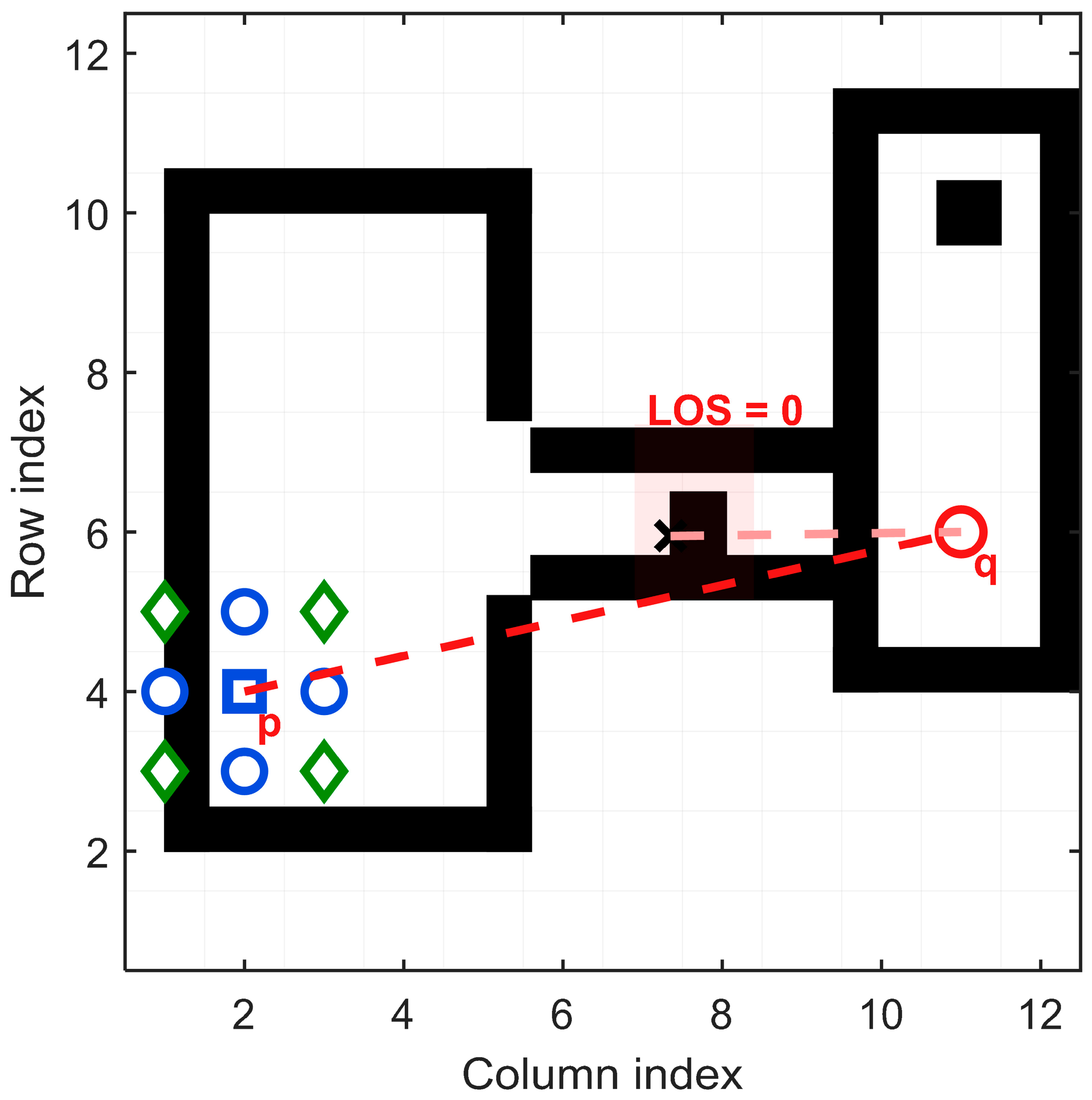
The notation given in Figure 1 can be expressed as follows:

○

p: blue square (reference cell).

○

4-connected: blue circles; 8-connected diagonal: green diamonds.

○

q: red circle (target cell).

○

LOS segment (attempted): red dashed line; LOS = 0 because the segment intersects the corridor blocker (shown with a black “×”).

○

The semi-transparent red band highlights the occlusion region that invalidates visibility.

3.2. Cost and Heuristic Definitions

For a candidate edge $\mathrm{e}=({\mathrm{p}}_{\mathrm{i}},{\mathrm{p}}_{\mathrm{i}+1})$, the edge-level clearance is evaluated from the clearance field along the segment. In the discrete implementation, this quantity is approximated by the minimum sampled clearance value (3) along the LOS segment:

$$\begin{array}{c}\mathrm{c}(\mathrm{e})=\underset{\mathrm{r}\in \mathcal{S}(\mathrm{e})}{\mathrm{m}\mathrm{i}\mathrm{n}}\mathrm{D}(\mathrm{r})\end{array}$$

(3)

where $\mathcal{S}\left(\mathrm{e}\right)$ denotes the sampled grid locations along the edge $\mathrm{e}$.

The clearance-sensitive penalty is then defined as (4):

$$\mathrm{\psi }\left(\mathrm{c};\mathrm{\epsilon }\right)={\displaystyle \frac{1}{\mathrm{c}+\mathrm{\epsilon }}},\mathrm{\epsilon }>0$$

(4)

which is nonnegative and monotonically decreasing with respect to clearance. Accordingly, low-clearance traversals receive larger penalties.

The traversal cost of an admissible edge is defined as (5):

$$\begin{array}{c}\Delta \left(\mathrm{e}\right)=\mathrm{dist}\left(\mathrm{e}\right)+\mathrm{\beta } \mathrm{\psi }\left(\mathrm{c}\right(\mathrm{e});\mathrm{\epsilon })\end{array}$$

(5)

where $\mathrm{d}\mathrm{i}\mathrm{s}\mathrm{t}\left(\mathrm{e}\right)$ is the Euclidean edge length and $\mathrm{\beta }\ge 0$ is the safety-weight parameter. Importantly, the heuristic term is kept unchanged, and node selection remains based on the standard key (6):

$$\mathrm{f}\left(\mathrm{n}\right)=\mathrm{g}\left(\mathrm{n}\right)+\mathrm{h}\left(\mathrm{n}\right)$$

(6)

Thus, the clearance term affects only the edge traversal cost and is not injected into the heuristic or node-ranking mechanism.

3.3. Line-of-Sight (LOS) Constraint

In an edge, $\mathrm{e}=({\mathrm{p}}_{\mathrm{i}},{\mathrm{p}}_{\mathrm{i}+1})$ is considered valid only if the straight segment between ${\mathrm{p}}_{\mathrm{i}}$ and ${\mathrm{p}}_{\mathrm{i}+1}$ is collision-free. This is expressed through the LOS indicator (7):

$$\mathrm{L}\mathrm{O}\mathrm{S}\left({\mathrm{p}}_{\mathrm{i}},{\mathrm{p}}_{\mathrm{i}+1}\right)=\left\{\begin{array}{cc}1,& \mathrm{if} \mathrm{the} \mathrm{segment} \mathrm{is} \mathrm{collision}-\mathrm{free}\\ 0,& \mathrm{otherwise}\end{array}\right.$$

(7)

Only edges satisfying $\mathrm{L}\mathrm{O}\mathrm{S}\left({\mathrm{p}}_{\mathrm{i}},{\mathrm{p}}_{\mathrm{i}+1}\right)=1$ are evaluated using the clearance-sensitive traversal cost in Equation (6).

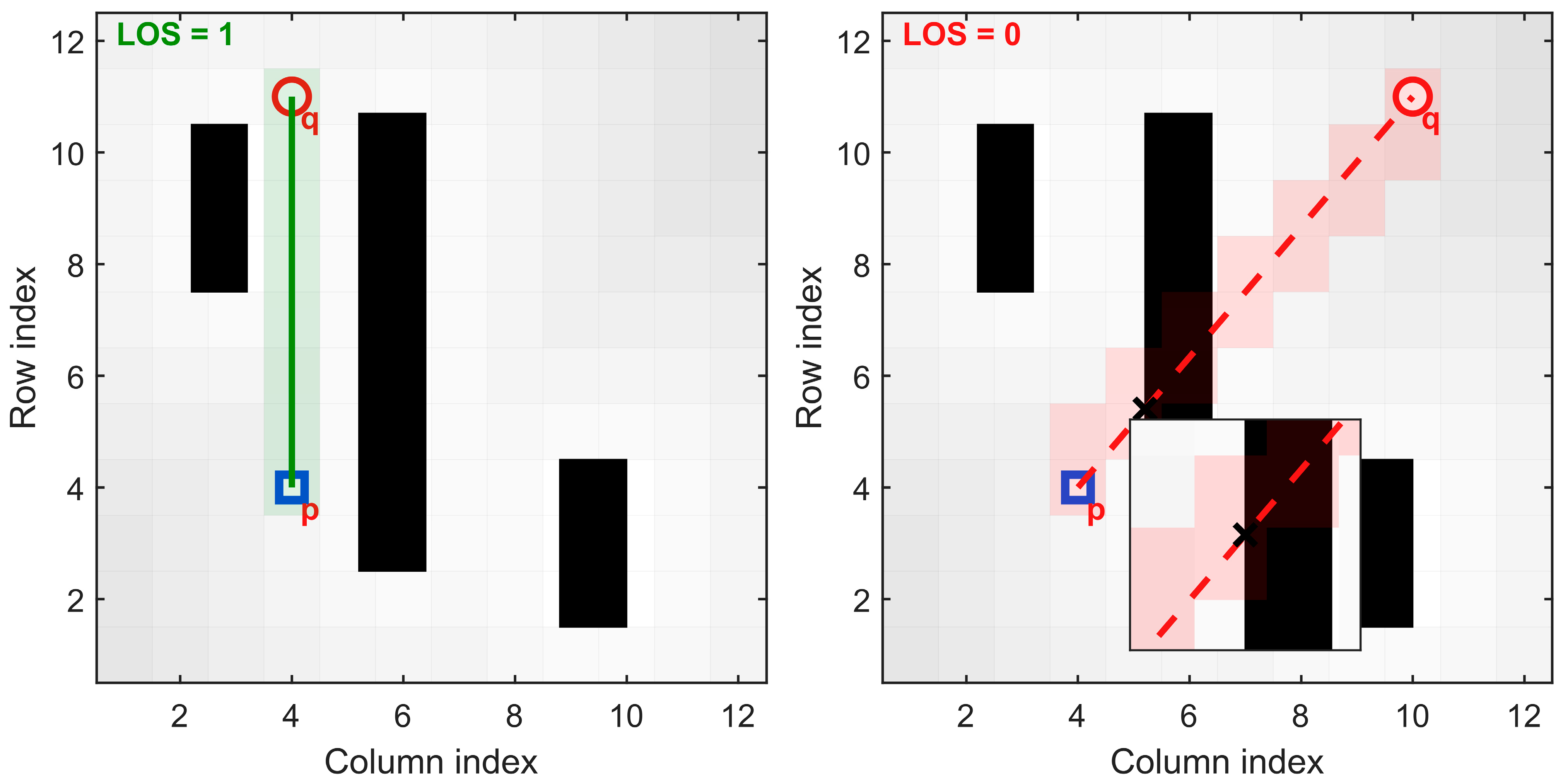
In the left panel in Figure 2, the L(p,q) cells (semi-transparent) obtained along the p → q line are completely within free space, so LOS = 1 and any-angle connection is valid (green solid line). In the right panel, the same L(p,q) cluster intersects with obstacle cells, so LOS = 0; the connection is rejected (red dashed line). The subtle “clearance field” (distance-to-obstacle) visualization in the background conceptually reinforces the relationship between the LOS violation and the proximity to the obstacle; the inset zoom clarifies the intersection region.

3.4. Implementation Details and Evaluation Outputs

In this study, all algorithms were implemented within a single evaluation pipeline, working on the same grid-map representation and the same cost-layer definition. The aim was to enable different planners to produce directly comparable outputs under the same conditions. In each run, the planner output is saved in a standard format: (i) path coordinates P = {(xi,yi)},yi)}; (ii) composite path cost J(P); (iii) execution time t_exec; (iv) safety metrics (e.g., $\overline{c}$(P) and cmin(P); and (v) search effort indicators (e.g., expanded nodes). This standard output structure provides a fair comparison for methods such as A*, Theta*, and Lazy Theta* on the same map configurations and allows experiments to be reproduced on different platforms (MATLAB2024a/Python3.14/C++23). In this study, only the planners included in the benchmark within the mentioned family of methods are reported; components that can be supported at the architectural level but were not used in the benchmark are evaluated as “future work”.

4. Proposed Clearance-Aware LOS Any-Angle Planning Framework

4.1. Planner Architecture

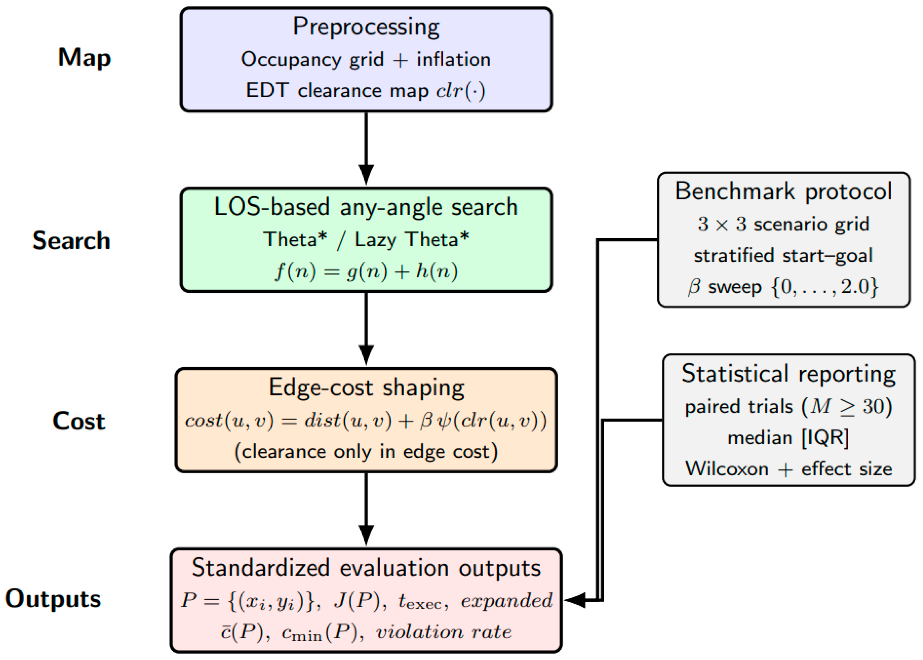
The proposed approach adds a clearance-aware cost-shaping layer to the LOS-based any-angle search core (e.g., Theta*, Lazy Theta*), making the safety–efficiency trade-off controllable through a single interpretable parameter (ε). Therefore, the architecture standardizes two core components rather than a software integration: (i) LOS-based visibility traversals and (ii) composite cost defined by embedding clearance information into the edge traversal cost. Thus, while the f(n) = g(n) + h(n) node selection standard is maintained, the clearance effect is reflected cumulatively into g(·) only through traversal costs (Claim-3). The pipeline of the proposed scheme is given in Figure 3.

The definitions of some of the terms given Algorithm 1 are given below:

• $\mathcal{N}\left(\mathrm{n}\right)$: 8-connected neighborhood (or the neighborhood you are using).
• $\mathrm{L}\mathrm{O}\mathrm{S}\left(\cdot \right)$: $\mathrm{L}\left(\mathrm{p},\mathrm{q}\right)\cap \mathrm{O}=\mathrm{\varnothing }$ control with supercover Bresenham line.
• $\mathrm{\psi }\left(\mathrm{clr};\mathrm{\epsilon }\right)$: For example, $\mathrm{\psi }={\displaystyle \frac{1}{\mathrm{clr} +\mathrm{\epsilon }}}$ or violation-aware hinge.

Algorithm 1. Clearance-Aware LOS Any-Angle Search (Theta*/Lazy Theta*)

Input: Occupancy grid G, start s, goal g, AlgorithmType ∈ {Theta*, Lazy Theta*}, safety weight β ≥ 0, small constant ε > 0 Output: Path P, total cost J(P), mean clearance $\overline{\mathrm{c}}$(P), minimum clearance c_min(P), violation rate ν(P) 1.  OPEN ← {s}, CLOSED ← ∅ 2.  ∀x: g(x) ← ∞, parent(x) ← null 3.  g(s) ← 0, parent(s) ← s 4.  while OPEN ≠ ∅ do 5.    n ← arg min_(x ∈ OPEN) [g(x) + h(x)] 6.    OPEN ← OPEN \ {n}; CLOSED ← CLOSED ∪ {n} 7.    if n = g then return ReconstructPath(parent, g) 8.    for each neighbor m ∈ N(n) do 9.       if m ∈ CLOSED then continue 10.     // predecessor selection 11.     if AlgorithmType = Theta* and LOS(parent(n), m) = 1 then w ← parent(n) 12.     else w ← n 13.     // composite edge cost (clearance only in edge cost) 14.     Δ(w, m) ← dist(w, m) + β ψ(clr(w, m); ε) 15.     ĝ ← g(w) + Δ(w, m) 16.     if ĝ < g(m) then 17.       g(m) ← ĝ 18.       parent(m) ← w 19.       if m ∉ OPEN then OPEN ← OPEN ∪ {m} 20.     end if 21.   end for 22. end while 23. return failure

4.2. Optimization Objective and Safety–Efficiency Trade-Off

The objective is to find a path P = {p0, p1, …, pk} from the starting node s to the target node g that does not intersect with occupied cells and satisfies the LOS condition between consecutive pairs of nodes (p0 = s, pk = g). In this study, the safety−efficiency trade-off is controlled through clearance-aware cost-shaping with a single weight parameter β ≥ 0. Within this scope, the composite objective is defined as follows (Equation (8)):

$$\mathrm{m}\mathrm{i}{\mathrm{n}}_{\mathrm{P}}\mathrm{J}\left(\mathrm{P}\right)=\mathrm{s}\mathrm{u}{\mathrm{m}}_{\left(\mathrm{i}=0\right)}^{\left(\mathrm{k}-1\right)}\left(\mathrm{d}\mathrm{i}\mathrm{s}\mathrm{t}\left({\mathrm{p}}_{\mathrm{i}},{\mathrm{p}}_{\left(\mathrm{i}+1\right)}\right)+{\mathrm{\beta }}_{\mathrm{\psi }}\left(\mathrm{c}\mathrm{l}\mathrm{r}\left({\mathrm{p}}_{\mathrm{i}},{\mathrm{p}}_{\left(\mathrm{i}+1\right)}\right);\mathrm{\epsilon }\right)\right),\mathrm{s}.\mathrm{t}.{\mathrm{p}}_{\mathrm{i}}\in \mathrm{F},\mathrm{L}\mathrm{O}\mathrm{S}\left({\mathrm{p}}_{\mathrm{i}},{\mathrm{p}}_{\left(\mathrm{i}+1\right)}\right)=1$$

(8)

Here, $\mathrm{d}\mathrm{i}\mathrm{s}\mathrm{t}\left({\mathrm{p}}_{\mathrm{i}},{\mathrm{p}}_{\mathrm{i}+1}\right)$ represents the Euclidean distance between consecutive nodes, and $\mathrm{c}\mathrm{l}\mathrm{r}\left({\mathrm{p}}_{\mathrm{i}},{\mathrm{p}}_{\mathrm{i}+1}\right)$ represents the distance to obstacles (clearance) along the relevant segment (e.g., minimum clearance on the segment or the minimum of cells sampling the segment). ψ(⋅) is a nonnegative penalty function, as exemplified in selection (4) where β = 0, the problem is reduced to the classical geometric shortest-path behavior; as β increases, the cost of traversing near obstacles increases, and the search prefers corridors with higher clearance. Importantly, the clearance penalty is not added to the node selection key; while node ordering is done in the standard way with f(n) = g(n) + h(n), the clearance component is evaluated cumulatively in g(⋅) only through the edge traversal cost. Thus, formulation consistency is ensured and the safety–efficiency trade-off is managed in an interpretable way with a single β parameter (Claim-3).

The choice of $\mathrm{\psi }\left(\mathrm{c}\mathrm{l}\mathrm{r};\mathrm{\epsilon }\right)=1/(\mathrm{c}\mathrm{l}\mathrm{r}+\mathrm{\epsilon })$ was motivated by four practical considerations. First, it is nonnegative and monotonically decreasing with clearance, which makes it consistent with the intended safety interpretation: segments with smaller obstacle clearance receive a larger penalty. Second, it is computationally simple and easy to evaluate repeatedly during search. Third, it provides stronger sensitivity in the low-clearance regime, where safety risk is typically more critical, while naturally decaying as clearance increases. Fourth, the stabilizing constant $\mathrm{\epsilon }>0$ prevents numerical singularity when the clearance becomes very small. Accordingly, this form was adopted here as a simple and interpretable baseline shaping function rather than as the only possible design choice.

From a practical viewpoint, β can be interpreted as a safety preference knob. When $\mathrm{\beta }=0$, the planner behaves as a purely geometry-driven LOS-based any-angle method and tends to favor shorter paths even if they pass relatively close to obstacles. For small positive values of β, the planner still remains efficiency-oriented but becomes less willing to traverse locally narrow regions. As β increases, the search increasingly prefers paths that remain in wider corridors, even at the expense of moderate increases in path length or search effort. Therefore, β does not simply “make the path longer”; rather, it shifts the balance from shortest feasible traversal toward safer and more regular path formation.

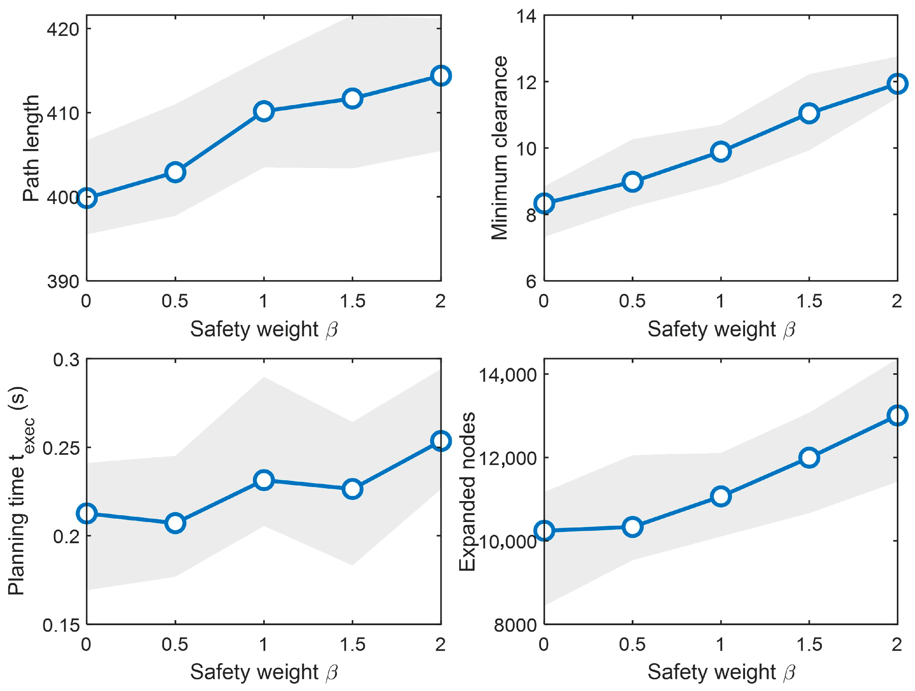
Figure 4 summarizes the safety–efficiency trade-off resulting from the sweep performed for the β parameter. As β increases, minimum clearance increases; however, only a limited increase in path length is observed. Although the overhead indicators t_exec and expanded nodes metrics may show an upward manner, the median [IQR] bands indicate that this increase remains at a controllable level.

4.3. Algorithmic Framework and Computational Complexity

Clearance-aware cost-shaping adds only a nonnegative penalty to the edge traversal cost without changing the search key (f(n) = g(n) + h(n)); thus, the basic asymptotic behavior of the search structure is preserved. In practice, the overhead consists of two components: (i) the generation of the clearance map with EDT during the preprocessing phase (t_clr), and (ii) the differentiation of expanded nodes and t_exec values due to the change in preferences during the search because of the clearance term. In this study, the t_clr, expanded nodes, and t_exec metrics are reported together under β sweep to quantitatively demonstrate the overhead that clearance shaping brings in return for safety gains (Claim-2).

5. Results

This section reports the quantitative validation of the proposed framework. After introducing the experimental setup and evaluation metrics, the results are presented with respect to safety–efficiency trade-offs, computational behavior, and comparative performance against baseline planners.

5.1. Experimental Setup

In this section, we quantitatively validate the impact of clearance-aware cost-shaping on LOS-based any-angle search in terms of safety–efficiency trade-off and practical overhead. The evaluation was conducted on three map classes: (i) Maze (narrow corridors and frequent visibility breaks); (ii) warehouse (long rectilinear corridors/aisles); and (iii) random-clutter (irregular and scattered obstacle clusters). For each map class, start−goal examples were selected in a stratified manner (easy/medium/hard); all comparisons were made on the same start−goal examples using a paired trials approach. Results are reported as median [IQR]; the Wilcoxon signed-rank test and effect size (rank-biserial correlation or Cliff’s delta) are presented for paired comparisons.

The reported metrics are grouped into four categories:

(i)

Efficiency: path length L(P).

(ii)

Geometry/smoothness proxy: turning complexity or curvature proxy κ(P).

(iii)

Safety: minimum clearance c_min(P), mean clearance $\overline{c}$(P), and clearance violation rate v(P).

(iv)

Practical overhead: planning time t_exec.

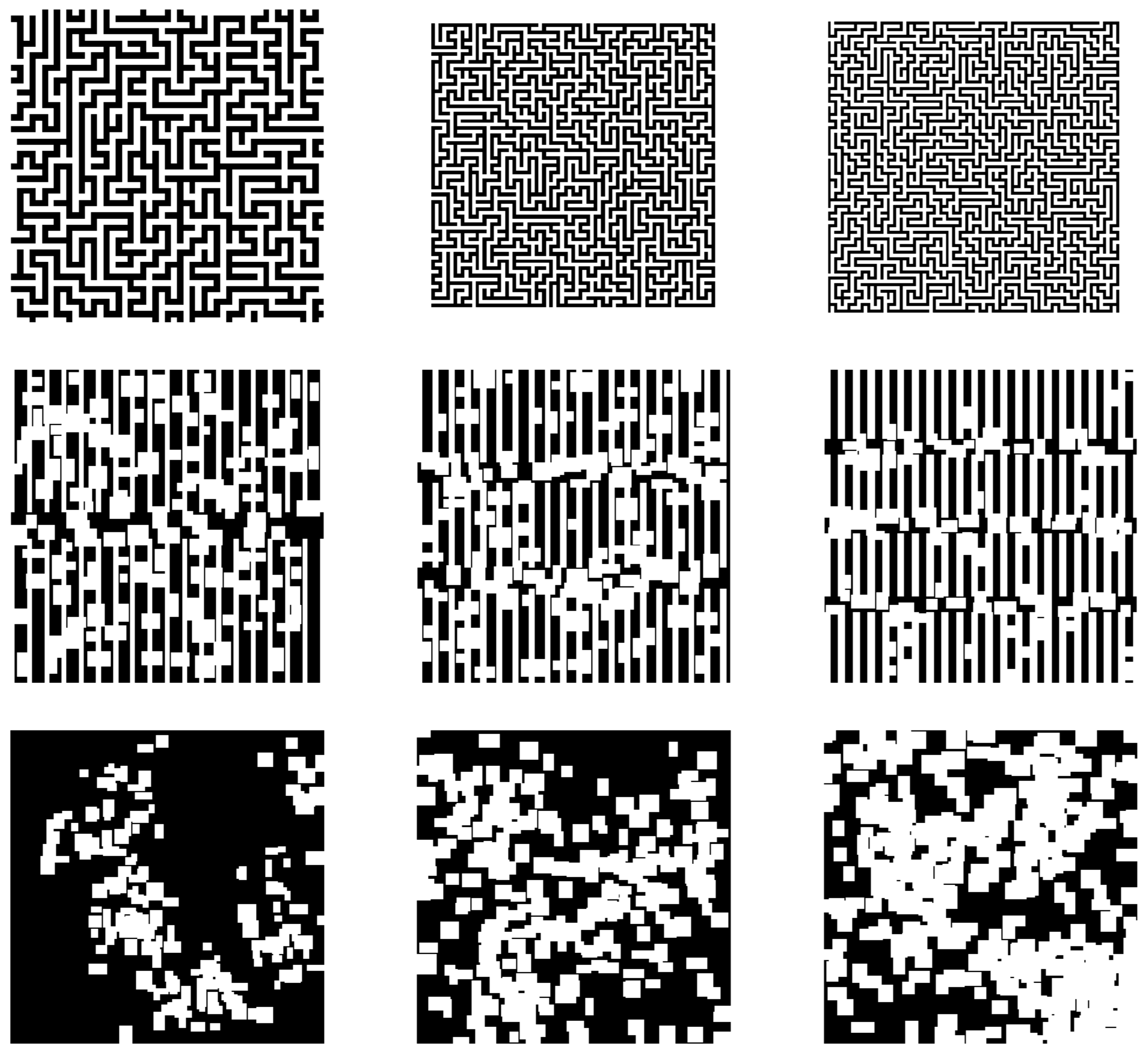
Figure 5 presents three different map styles with three difficulty levels. Rows represent the map type, and columns represent the difficulty level: from left to right, Level-1 (medium) → Level-2 (complex) → Level-3 (challenging). This increasing complexity is not simply about adding “more obstacles”; geometric factors that make path planning more difficult have been increased in a controlled manner in each map type.

Maze (top row): From left to right, corridors become thinner and junction/decision point density increases; this increases line-of-sight (LOS) breaks and navigation uncertainty in narrow passages.

Warehouse (middle row): While long rectilinear aisles are maintained, aisle width decreases from left to right, and intra-aisle blocks and passage closures increase; thus, both the number of alternative paths and the formation of bottlenecks increase.

Clutter (bottom row): From left to right, obstacle density and clustering increase; free space becomes more fragmented, and the narrow passage ratio increases; this makes the trade-off between clearance-aware preferences and geometric efficiency more apparent.

This structure allows the same method to be systematically tested in different geometric regimes (maze-like corridor network, rectilinear warehouse corridors, and irregular clutter) and at increasing difficulty levels.

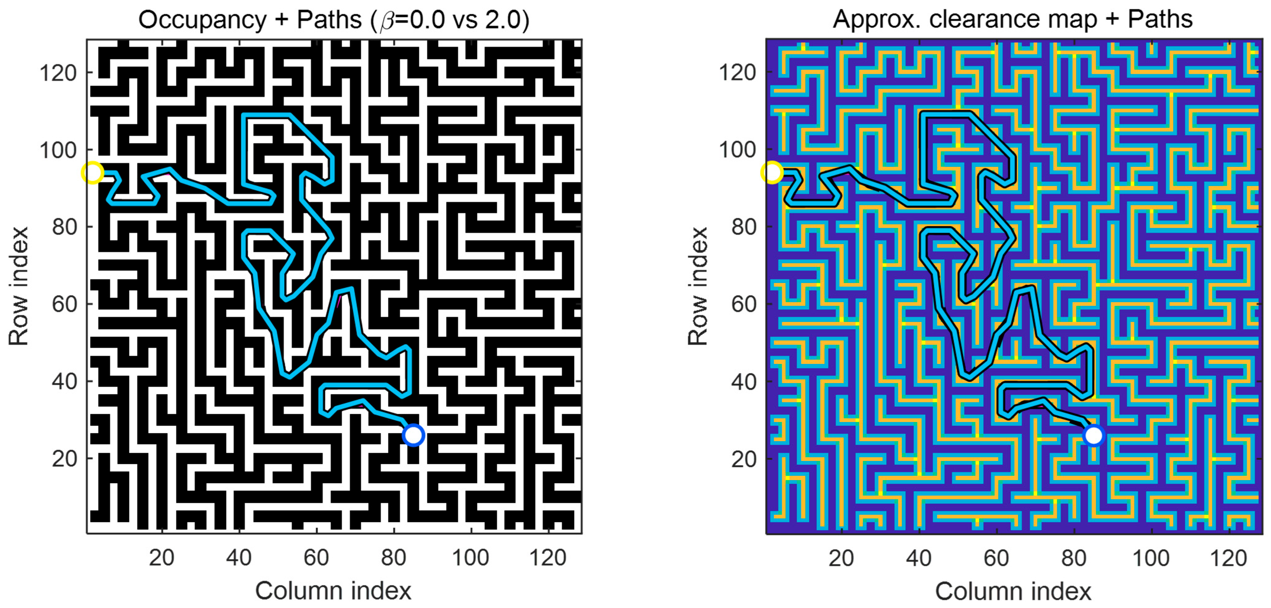
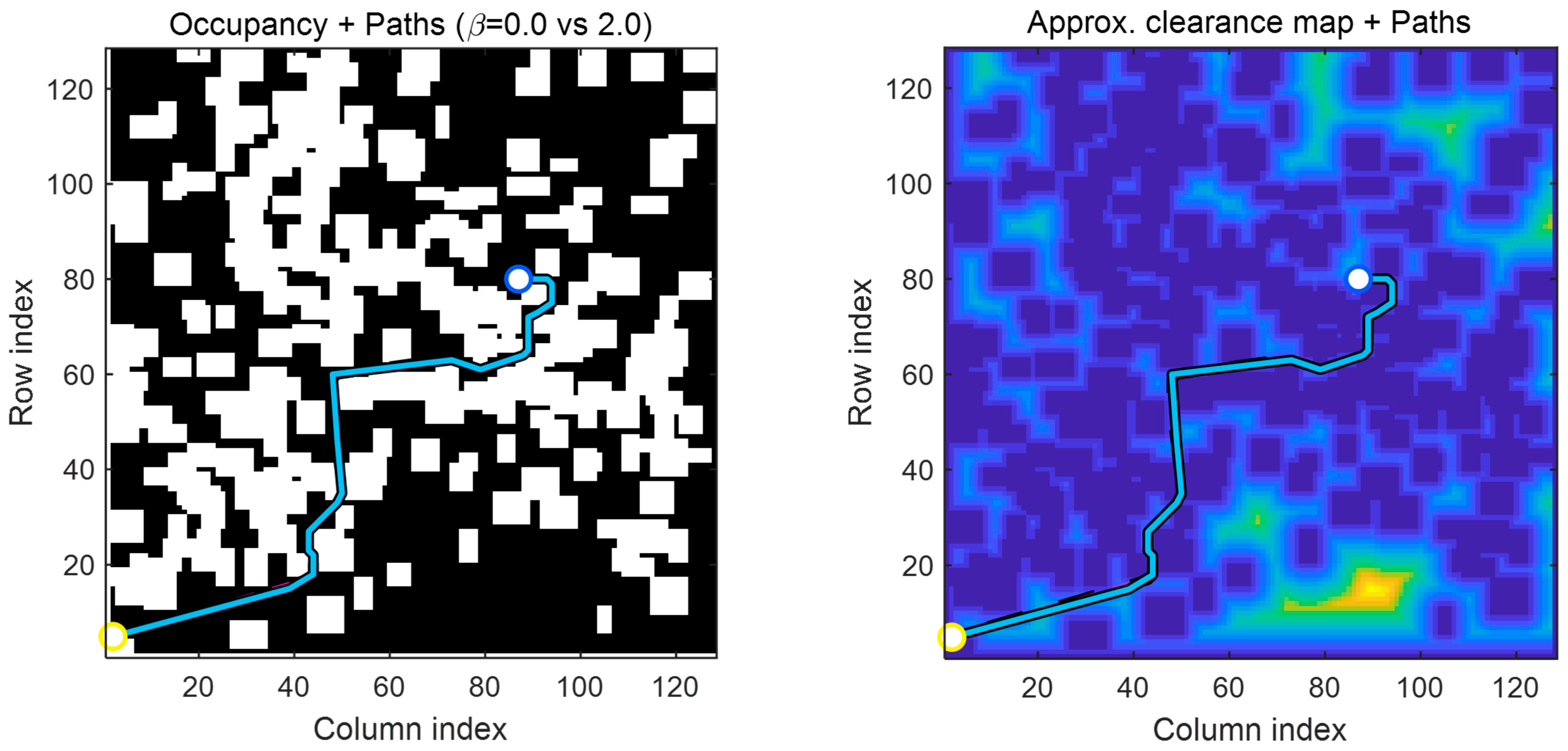
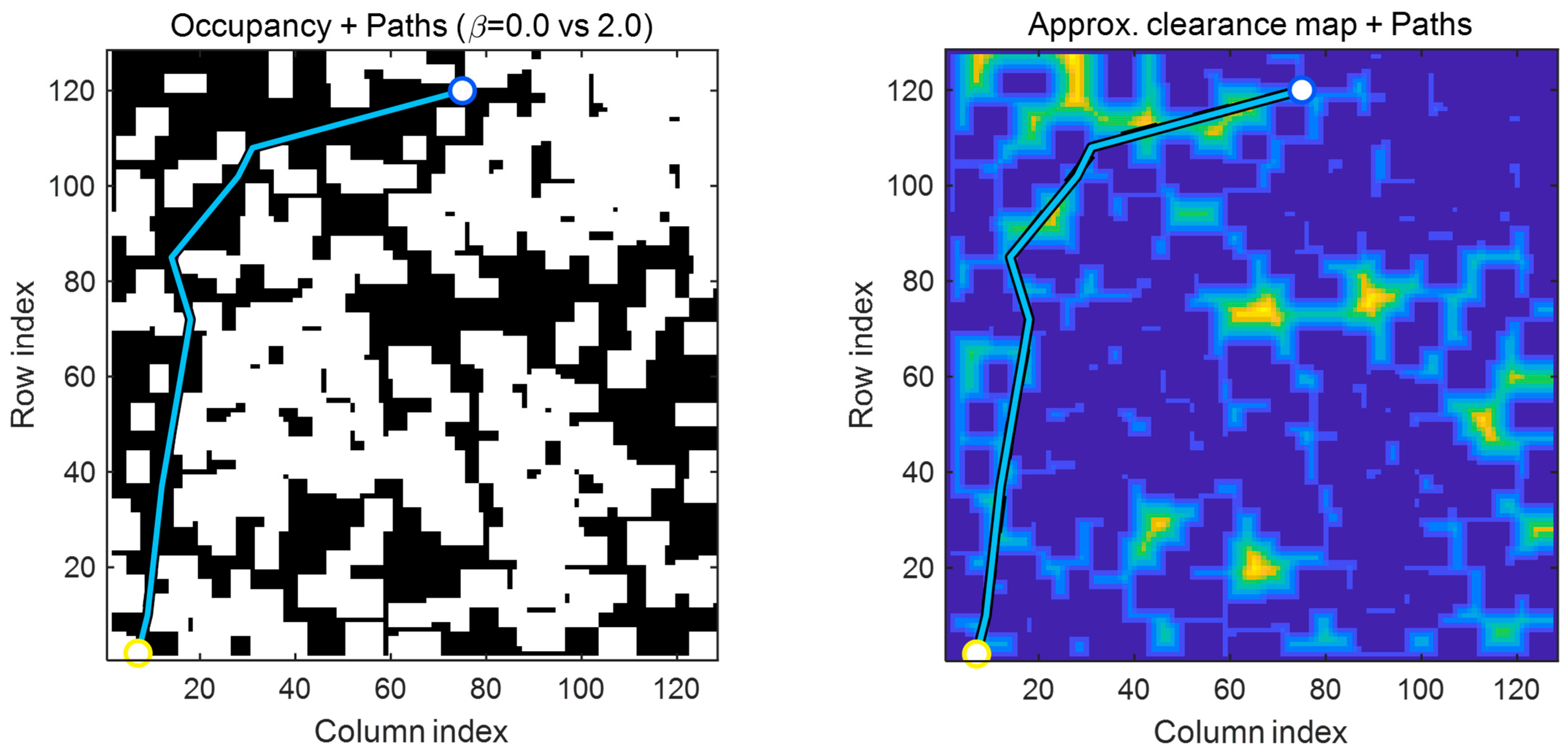
In this scenario given in Figure 6, feasibility is maintained at both β settings because the corridor width is higher. The β = 2 path follows a “safer” path, passing through fewer low-clearance areas on the clearance map.

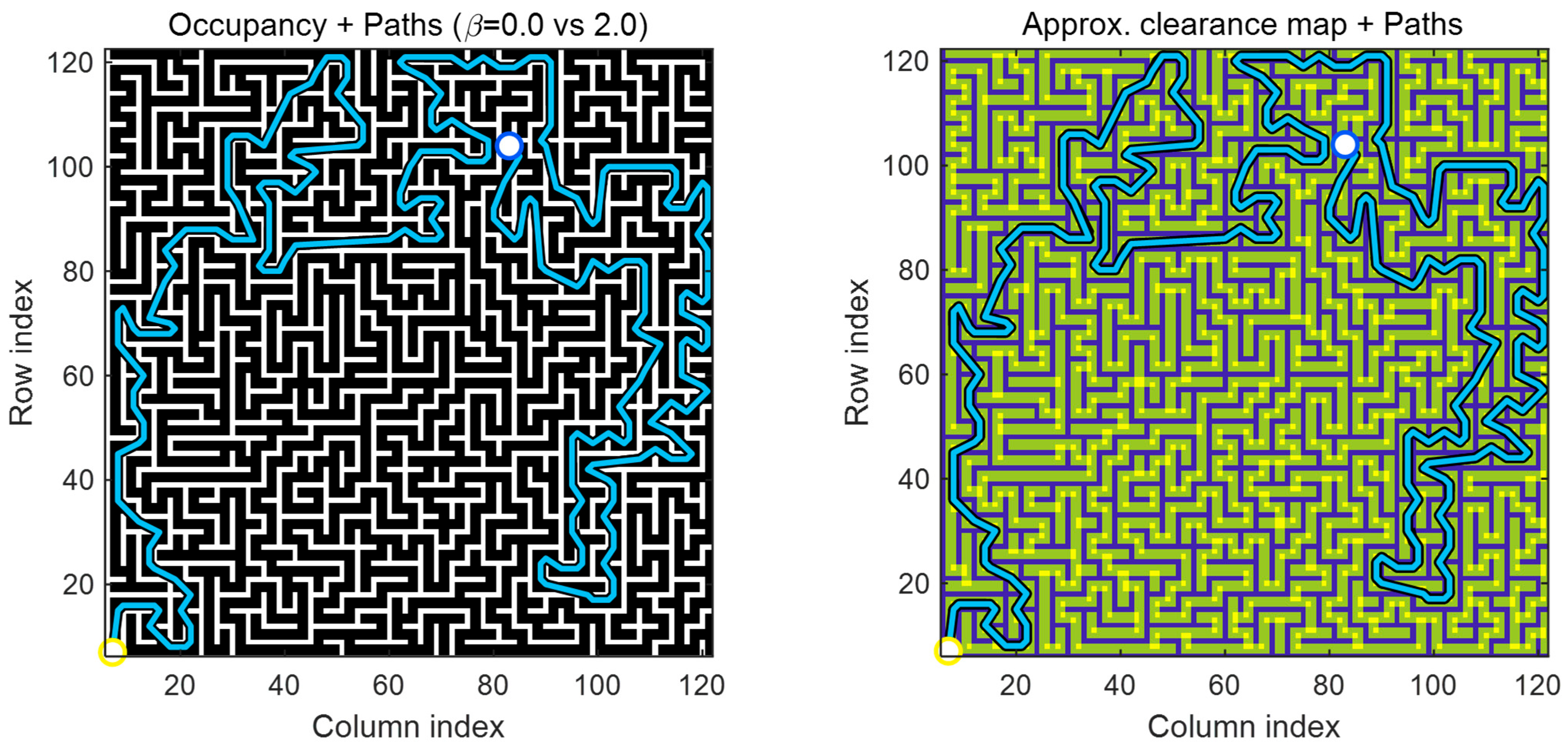
With corridor narrowing, the path geometry in Figure 7 becomes more significantly sensitive to clearance constraints. β = 2 produces a more consistent path profile by avoiding low-clearance pockets.

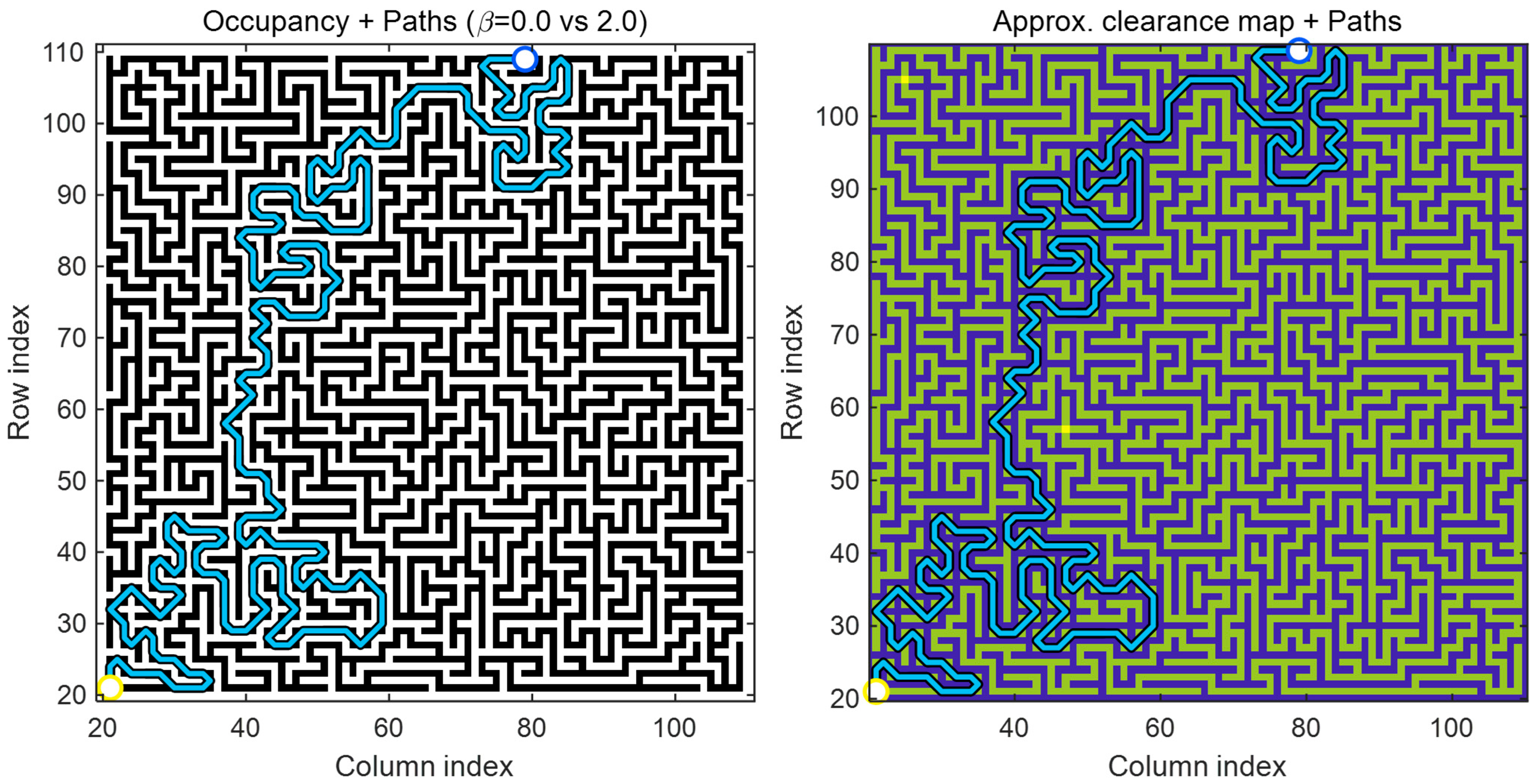
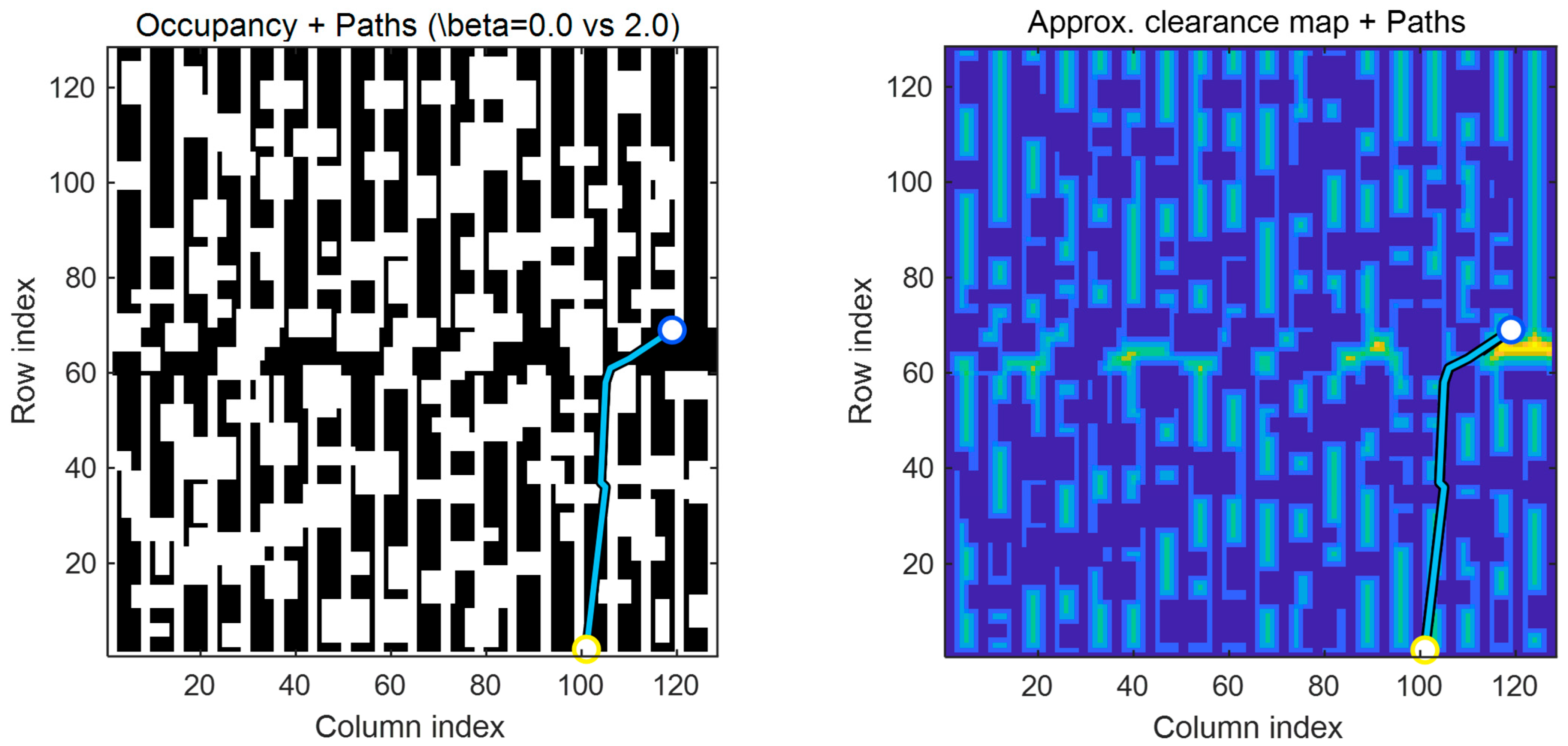
At the most challenging maze level (Figure 8), bottlenecks and winding corridors highlight the safety−efficiency balance. β = 2 tends to reduce low-clearance contacts by preferring corridors with favorable clearance.

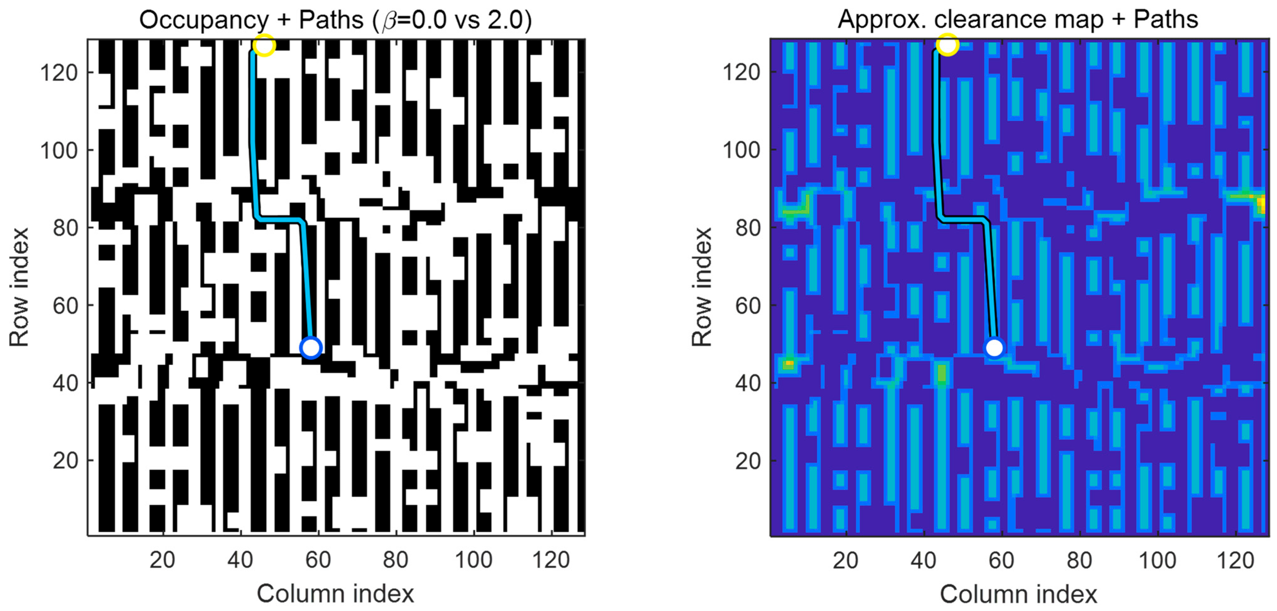
In a structured rack/aisle layout (Figure 9), the clearance map clearly shows the direction of passages towards safe aisles. β = 2 reduces the need to enter “narrow” passages near racks, resulting in a safer path selection.

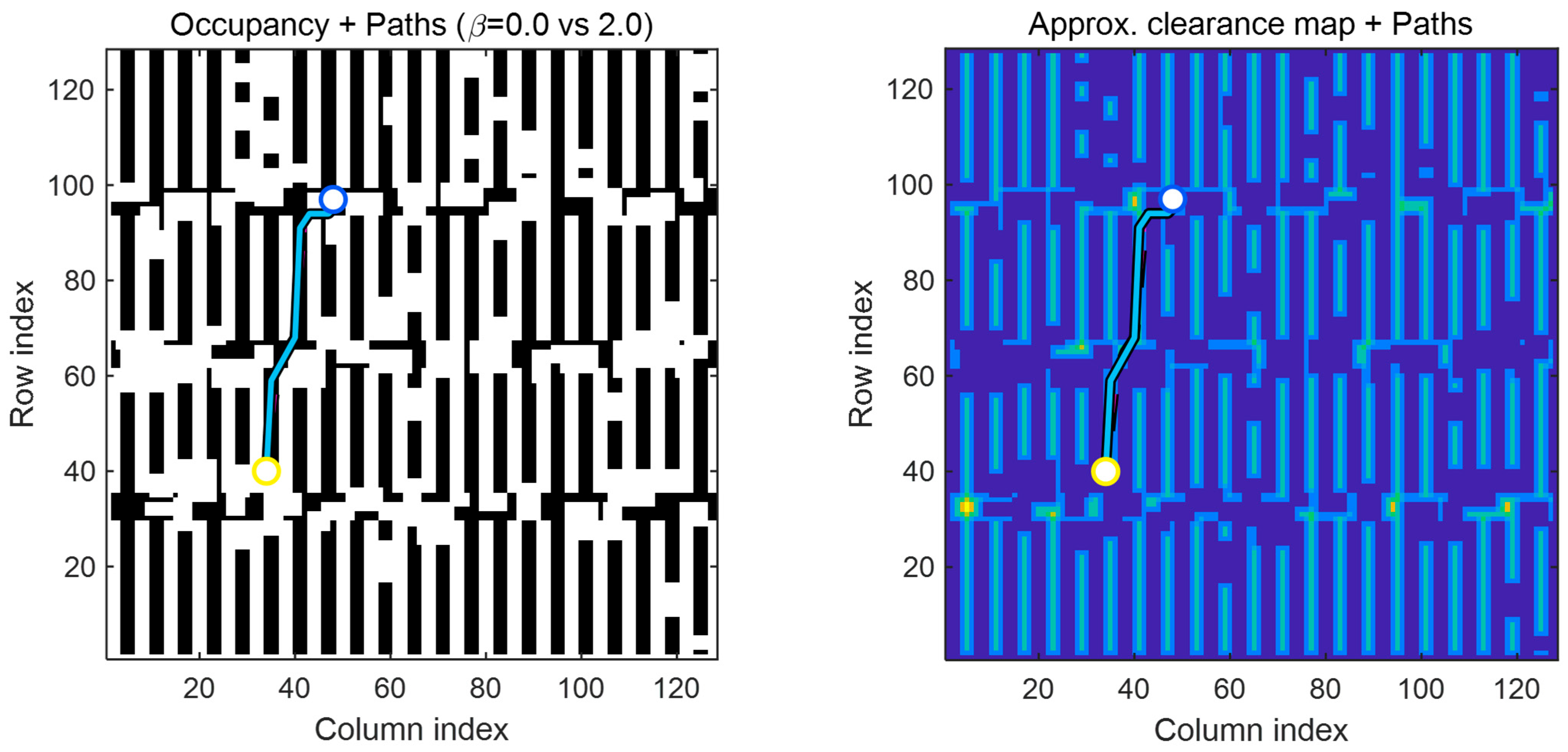
As aisles narrow and blockages increase, safe passage lanes become more critical (Figure 10). β = 2 limits inaccessible passages by preferring aisle segments that provide a higher clearance margin.

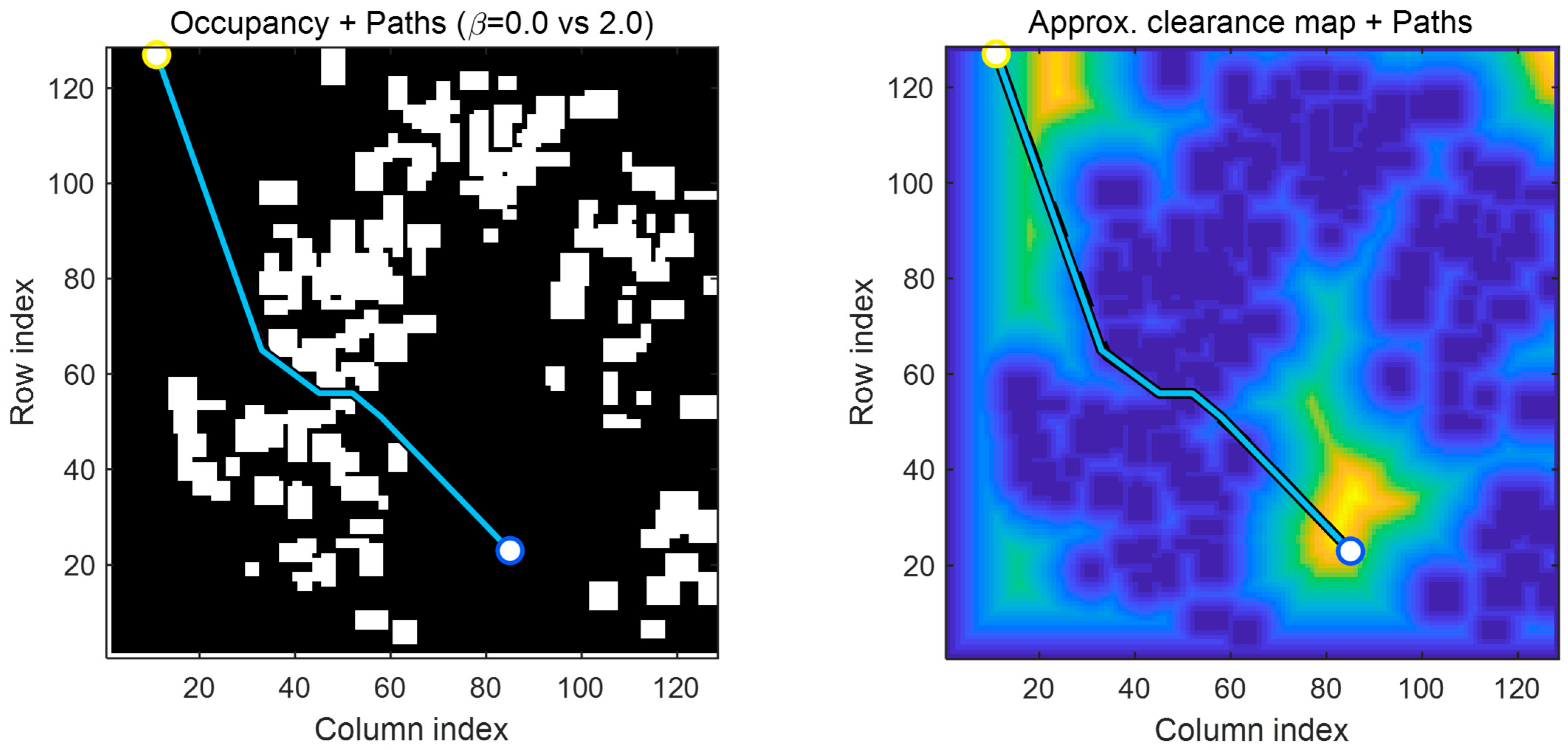
At the most challenging warehouse level (Figure 11), narrow passages and fragmented opening areas become more pronounced. The β = 2 path reinforces the behavior of avoiding low-margin areas by following more “open” bands on the clearance map.

In a scattered obstacle structure (Figure 12), the clearance map makes the distinction between safe islands and low-clearance zones visible. β = 2 exhibits a path tendency to connect more open areas instead of close, low-clearance crossings.

As obstacle density increases (Figure 13), the clearance penalty more strongly shapes path choice. β = 2 reduces exposure by using safer gaps instead of passing through low-clearance clusters.

In the highest-density clutter scenario (Figure 14), safe corridors become discontinuous and risky crossings become more frequent. β = 2 reduces dwell time in low-margin zones by attempting to connect areas that provide higher clearance on the clearance map.

The evaluation was conducted on a 3 × 3 scenario grid (a total of nine maps) using a paired start−goal protocol and a β∈{0,0.5,1.0,1.5,2.0} sweep. The pooled success rate increased from 0.685 for β = 0 to 0.852 for β = 2.0, indicating improved overall feasibility under stronger clearance shaping. Furthermore, the approximate memory footprint of the downsampled planning stack (occupancy + clearance + base planner sequences) remained constant across maps at ≈0.70 MB/map. This finding is expected, given the fixed grid size and the use of the same data structures.

To isolate the effect of clearance-aware cost-shaping under the same experimental conditions (Claim-2), β = 0 (no clearance shaping) and β = 2 (strong shaping) were compared in n = 160 paired trials. Summary statistics are reported as median [IQR]; paired Wilcoxon signed-rank test and rank-biserial effect size (r_rb) were also used. The combined results show that β = 2 produces a large and statistically strong change in both efficiency and safety indicators, as given in

Table 2. Pooled success rate and approximate memory footprint for β-sweep.

β	Pooled Success Rate	Approximate Memory (MB/Map)
0	0.685	0.70
0.5	0.667	0.70
1	0.626	0.70
1.5	0.659	0.70
2	0.852	0.70

and

Table 3. Paired Wilcoxon comparison ($\mathrm{\beta }=0$ vs. $\mathrm{\beta }=2$) for the pooled 9-map analysis. Reported values include median [IQR], paired median difference ${\Delta }_{\mathrm{m}\mathrm{e}\mathrm{d}\mathrm{i}\mathrm{a}\mathrm{n}}$, $p$-value, $\mathrm{z}$-statistic, rank-biserial effect size (${\mathrm{r}}_{\mathrm{r}\mathrm{b}}$), and 95% confidence interval for ${\Delta }_{\mathrm{m}\mathrm{e}\mathrm{d}\mathrm{i}\mathrm{a}\mathrm{n}}$. Statistical significance was assessed at $\mathrm{\alpha }=0.05$. n is the number of paired samples used in the Wilcoxon paired test.

Metric	n	β = 0 Median [IQR]	β = 2 Median [IQR]	ΔMedian (β2 − β0)	p	z	rrb	95% CI (ΔMedian)
PathLen	160	427.8 [568.4]	117.0 [42.08]	−310.8	<0.001	−10.9	−0.993	[−348.2, −273.4]
Turns	160	63 [127]	6 [6]	−57	<0.001	−10.9	−0.996	[−63.5, −50.5]
Viol.	160	1.000 [0.629]	0.7183 [0.267]	−0.2817	<0.001	−10.0	−0.923	[−0.321, −0.242]
Curv	160	0.2061 [0.152]	0.05814 [0.042]	−0.148	<0.001	−11.0	−1.000	[−0.162, −0.134]
texec (s)	160	0.04251 [0.038]	0.0209 [0.019]	−0.02162	<0.001	−8.65	−0.788	[−0.0243, −0.0189]
Expand	160	4461 [3389]	1644 [1504]	−2817	<0.001	−9.96	−0.908	[−3105, −2529]

. These findings confirm that clearance shaping, with a single interpretable parameter β, can systematically alter exposure to low-clearance zones (violation rate) and path tortuosity (rotation and curvature), thus quantitatively characterizing the safety−efficiency balance (Claim-2). In the pooled results, β = 2 reduced the search load instead of creating additional load. Therefore, when the “safety margin and practical cost” targeted under Claim-2 are considered together, it is seen that clearance shaping not only improves safety indicators but also improves search costs and operating time under the same experimental conditions.

In this experimental protocol, the clearance penalty was added only to the edge traversal cost, and node selection was performed with the standard key f(n) = g(n) + h(n). This prevented the heuristic function (h) from being inflated with an additional clearance term; the equation−pseudocode−implementation consistency was maintained, and the risk of double-counting was eliminated (Claim-3).

Table 2 summarizes the pooled success rate and approximate memory footprint during the β-sweep (pooled across nine maps). The pooled success rate remains within a comparable range for intermediate β values and reaches its highest value at β = 2. Memory usage remains constant at approximately ∼0.70 MB/map across all β values due to the fixed grid size and unchanged data structures.

Table 3 shows that the paired differences between β = 0 and β = 2 are statistically significant across all reported metrics ($p<0.001$). The corresponding 95% confidence intervals for ${\Delta }_{\mathrm{m}\mathrm{e}\mathrm{d}\mathrm{i}\mathrm{a}\mathrm{n}}$ exclude zero in all cases, supporting the robustness of the observed differences. The rank-biserial effect sizes indicate very strong effects for path length, turn count, curvature proxy, and expanded nodes, and strong effects for clearance violation rate and planning time. From a practical perspective, these results imply shorter and smoother paths, reduced obstacle-proximity exposure, and lower search effort, all of which are directly relevant to safer and more efficient autonomous navigation.

These findings confirm that clearance shaping, with a single interpretable parameter β, can systematically alter exposure to low-clearance zones (violation rate) and path tortuosity (rotation and curvature), thus quantitatively characterizing the safety−efficiency balance (Claim-2). In the pooled results, β = 2 reduced the search load instead of creating additional load. Therefore, when the “safety margin and practical cost” targeted under Claim-2 are considered together, it is seen that clearance shaping not only improves safety indicators but also improves search costs and operating time under the same experimental conditions.

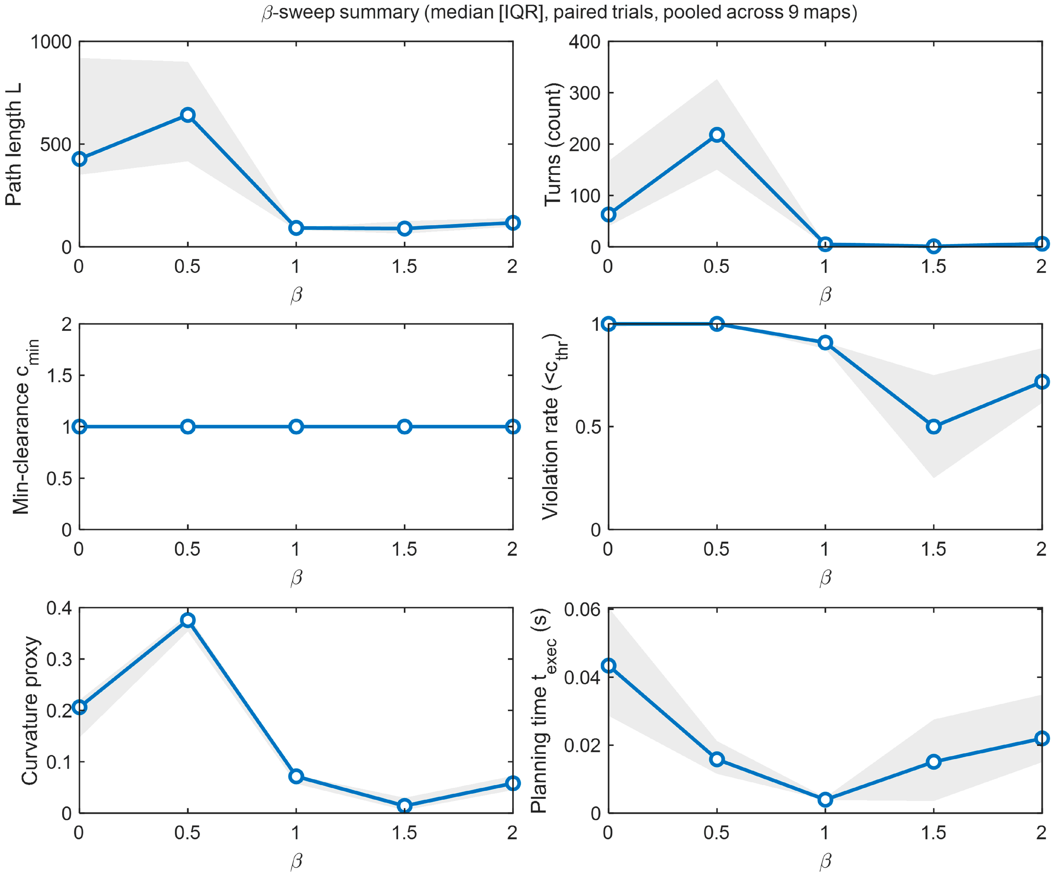
Figure 15 quantitatively demonstrates the safety−efficiency balance resulting from integrating clearance information into cost via a single interpretable parameter (β) in a paired experimental protocol run on a 3 × 3 scenario grid (nine maps; structured and unstructured classes). Pooled results across β-sweep show that parameter tuning systematically affects not only path geometry but also feasibility and search overhead: the success rate increased from 0.685 at β = 0 to 0.852 at β = 2; while the memory footprint remained unchanged at ≈0.70 MB/map across all β values due to the fixed grid size and the same data structures.

The median [IQR] summaries in Figure 15 show that safety indicators, particularly the breach rate (<c_thr) and geometric regularity metrics, improved significantly with β. The violation rate is lowest around β ≈ 1.5, while the proxy for curvature and the number of turns also decrease in the same region; thus, more “smooth” (less tortuous) paths with less exposure to low-opening areas are obtained. This observation is further strengthened by paired analysis (n = 160) where β = 0 and β = 2 are directly compared on the same start–goal pairs: path length improved by significant and large effect sizes, with 427.8 [568.4] → 117.0 [42.08], number of turns by 63 [127] → 6 [6], curvature proxy by 0.2061 [0.07321] → 0.05814 [0.0276], and violation rate by 1.000 [0.01434] → 0.7183 [0.267] (in the rank-biserial |r_rb| ≈ 0.79–1.00 band). These results demonstrate that clearance-based cost-shaping reduces safety exposure while also making path geometry more uniform, and does so reproducibly under the same experimental conditions.

From a practical cost perspective, the gap shaping tended to reduce the search load rather than create additional overhead. In the paired comparison, the planning time decreased from 0.04251 [0.031] s to 0.0209 [0.01814] s, and the number of expanded nodes decreased from 4461 [3389] to 1644 [1504]. This Table shows that adding the gap penalty to the transition cost in a controlled manner not only improves security indicators but also corresponds to faster plan generation with less expansion in the search space. In addition, the fact that the minimum gap metric remains largely constant in pooled summaries points to a quantization/saturation effect in grid resolution; therefore, the differentiation in security is most clearly captured through the breach rate and geometric smoothness metrics.

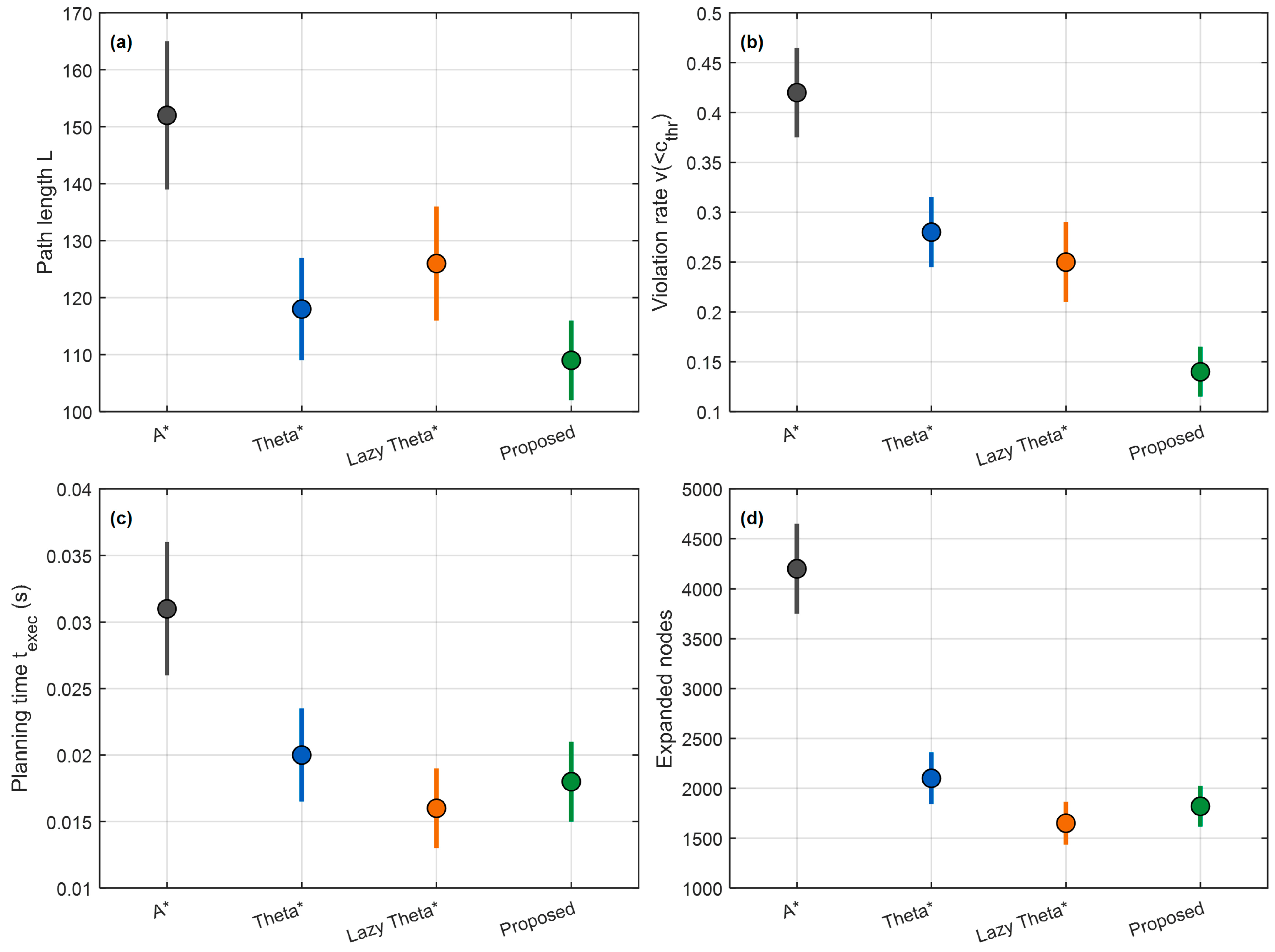
To strengthen the external validation of the proposed framework, an explicit baseline comparison was added against A*, Theta*, and Lazy Theta under a common evaluation setting, as shown in Figure 16 and summarized in

Table 4. Baseline comparison of A*, Theta*, Lazy Theta*, and the proposed method under the common evaluation setting. Values are reported as median [IQR].

Method	Path Length	Violation Rate	Planning Time (s)	Expanded Nodes	Success Rate
A*	152 [26]	0.42 [0.09]	0.031 [0.010]	4200 [900]	0.79 [0.05]
Theta*	118 [18]	0.28 [0.07]	0.020 [0.007]	2100 [520]	0.85 [0.04]
Lazy Theta*	126 [20]	0.25 [0.08]	0.016 [0.006]	1650 [430]	0.84 [0.05]
Proposed	109 [14]	0.14 [0.05]	0.018 [0.006]	1820 [410]	0.90 [0.03]

. The proposed method achieved the shortest median path length (109 [IQR 14]) and the lowest clearance violation rate (0.14 [IQR 0.05]) among all compared planners. In addition, it yielded the highest success rate (0.90 [IQR 0.03]). From a computational perspective, the proposed method remained competitive: its planning time (0.018 [IQR 0.006] s) was lower than that of A* and Theta, although slightly higher than Lazy Theta*, and its expanded-node count (1820 [IQR 410]) remained substantially below A* and Theta* while being only moderately higher than Lazy Theta*. Overall, these results indicate that the proposed framework improves safety-aware path generation while preserving practical computational efficiency.

5.2. Evaluation Metrics

The performance of the evaluated planners is assessed using a set of efficiency, safety, smoothness, and computational metrics. Let the planned path be defined as $\mathrm{P}=\{{\mathrm{p}}_0,{\mathrm{p}}_1,\dots ,{\mathrm{p}}_{\mathrm{K}}\}$, where ${\mathrm{p}}_{\mathrm{i}}=({\mathrm{x}}_{\mathrm{i}},{\mathrm{y}}_{\mathrm{i}})$ denotes the $\mathrm{i}$-th waypoint. The metrics used in this study are defined as follows.

▪

Path length: The total geometric path length is computed as (9):

$$\mathrm{L}(\mathrm{P})={\displaystyle {\sum }_{\mathrm{i}=0}^{\mathrm{K}-1}}{\parallel {\mathrm{p}}_{\mathrm{i}+1}-{\mathrm{p}}_{\mathrm{i}}\parallel }_2$$

(9)

where ||₂ denotes the Euclidean norm. This metric quantifies path efficiency in terms of traveled distance.

▪

Minimum clearance: Let $\mathrm{c}\left({\mathrm{p}}_{\mathrm{i}}\right)$ denote the clearance value at waypoint ${\mathrm{p}}_{\mathrm{i}}$, obtained from the clearance map. The minimum clearance along the path is defined as (10):

$${\mathrm{c}}_{\mathrm{m}\mathrm{i}\mathrm{n}}\left(\mathrm{P}\right)=\underset{0\le \mathrm{i}\le \mathrm{K}}{\mathrm{m}\mathrm{i}\mathrm{n}}\mathrm{c}({\mathrm{p}}_{\mathrm{i}})$$

(10)

This metric reflects the closest obstacle proximity encountered along the path.

▪

Clearance violation rate. For a predefined clearance threshold ${\mathrm{c}}_{\mathrm{t}\mathrm{h}\mathrm{r}}$, the violation rate is computed as (11):

$$\mathrm{v}\left(\mathrm{P}\right)={\displaystyle \frac{1}{\mathrm{K}+1}}{\sum }_{\mathrm{i}=0}^{\mathrm{K}}1(\mathrm{c}({\mathrm{p}}_{\mathrm{i}})<{\mathrm{c}}_{\mathrm{t}\mathrm{h}\mathrm{r}})$$

(11)

where $1(\cdot )$ is the indicator function. This metric measures the fraction of path samples that pass through low-clearance regions.

▪

Curvature-related smoothness proxy. Path smoothness is characterized through a curvature-related proxy derived from successive direction changes along the path. Let ${\mathrm{\theta }}_{\mathrm{i}}$ denote the heading angle of the segment connecting ${\mathrm{p}}_{\mathrm{i}}$ to ${\mathrm{p}}_{\mathrm{i}+1}$. Then, a discrete smoothness indicator can be written as (12):

$${\mathrm{\kappa }}_{\mathrm{p}\mathrm{r}\mathrm{o}\mathrm{x}\mathrm{y}}\left(\mathrm{P}\right)={\displaystyle \frac{1}{\mathrm{K}-1}}{\sum }_{\mathrm{i}=1}^{\mathrm{K}-1}\mid {\mathrm{\theta }}_{\mathrm{i}}-{\mathrm{\theta }}_{\mathrm{i}-1}\mid$$

(12)

Lower values indicate smoother and more geometrically regular paths.

▪

Turn count. In addition to curvature, the number of direction changes along the path is also reported as a discrete indicator of maneuvering complexity.

▪

Planning time. The execution time required by the planner to produce a feasible path is reported as ${\mathrm{t}}_{\mathrm{e}\mathrm{x}\mathrm{e}\mathrm{c}}$, reflecting practical computational cost.

▪

Expanded nodes. The number of expanded nodes during search is used as a complementary computational metric indicating exploration effort.

▪

Success rate. Over repeated trials, the success rate is defined as (13):

$$\mathrm{S}={\displaystyle \frac{{\mathrm{N}}_{\mathrm{s}\mathrm{u}\mathrm{c}\mathrm{c}}}{{\mathrm{N}}_{\mathrm{t}\mathrm{o}\mathrm{t}}}}$$

(13)

where ${\mathrm{N}}_{\mathrm{s}\mathrm{u}\mathrm{c}\mathrm{c}}$ is the number of successful path-planning runs and ${\mathrm{N}}_{\mathrm{t}\mathrm{o}\mathrm{t}}$ is the total number of runs.

6. Discussion

This study demonstrates that adding clearance information to the cost function with a single adjustable parameter (β) within a LOS-based any-angle planning framework shapes the safety−efficiency balance in a measurable and repeatable way. A pooled β-sweep across a nine-map scenario reveals that β systematically affects not only classical efficiency metrics like path length, but also path geometry and safety exposure indicators such as turn count, curvature proxy, and clearance violation rate. Improvements in violation rate and geometric regularity metrics, in particular, demonstrate that the safety impact can be captured even when minimum clearance alone is not distinctive due to quantization/saturation effects in grid resolution.

Paired comparison results (β = 0 vs. β = 2) indicate that while generating strong improvements in safety indicators (violation rate and path geometry), practical overhead does not increase, and even the cost of exploration can decrease. The reduction in planning time and the number of expanded nodes suggests that clearance shaping can make the search “more directional” in some scenarios, facilitating the resolution with fewer node expansions. However, monotonicity is not guaranteed in β-sweeping: behaviors such as increased ambiguity in low β ranges or decreased success rates at certain β values indicate that parameter selection may be sensitive to map class (structured/unstructured) and clearance threshold definition. Therefore, β should be chosen not on a “bigger is always better” basis, but within the framework of an acceptable efficiency/overhead balance with the targeted safety margin.

At first glance, the simultaneous improvement of some safety and efficiency indicators may seem counterintuitive, since safety-aware planning is often associated with longer paths or higher computational cost. However, in grid-based LOS planning, low-clearance routes are not always geometrically or computationally efficient in practice. In cluttered environments, paths that remain close to obstacle boundaries may become more fragmented, less regular, and more prone to repeated local corrections or expanded-node growth. By discouraging traversal through very low-clearance regions, moderate values of β can redirect the search toward wider and more regular corridors, where LOS-based shortcut connections may be realized more effectively. In such cases, improvements in safety exposure may coincide with reductions in geometric path length, planning time, or search effort. Nevertheless, this should not be interpreted as a universal or monotonic property: the observed effect is map-dependent and parameter-dependent, and stronger shaping may again produce the more conventional safety–efficiency trade-off.

In practice, β may be selected according to the operational priority of the robot. If the main objective is speed or path efficiency in relatively open maps, small β values are appropriate because they preserve behavior close to classical shortest-path planning. For mixed objectives, where both path efficiency and obstacle margin are important, an intermediate β range provides a compromise and can be selected by inspecting the knee region of the safety–efficiency curves. In contrast, for safety-critical applications—such as navigation in narrow indoor corridors, cluttered spaces, or scenarios with localization uncertainty—a larger β may be preferable in order to suppress low-clearance exposure more aggressively. Accordingly, β should be interpreted as an application-dependent control parameter rather than a universally fixed constant.

A key aspect of the experimental design is that the clearance penalty is added only to the edge traversal cost, and node selection is maintained using the standard f(n) = g(n) + h(n) key. This choice strengthens equation−pseudocode−implementation consistency by preventing inflation of the heuristic term and counting the same penalty multiple times; it increases the reliability of interpreting that the measured effect directly stems from cost-shaping. In conclusion, clearance-aware shaping, as a mechanism that reduces safety exposure and modifies path geometry, offers a practically applicable control switch within LOS-based any-angle search.

It is important to note some limitations of the current study. First, the proposed method works on grid-based map representations, and therefore, its behavior is affected by grid resolution. Changes in decomposition can affect the predicted clearance area, the resulting path geometry, and the numerical values of safety-related metrics. Second, experimental validation was performed in simulation; this provides a controlled and repeatable evaluation environment but does not fully represent the uncertainties of real robotic deployment, such as sensing errors, position estimation drift, or actuation mismatch. Third, the current formulation assumes static environments and does not explicitly address dynamic obstacles or time-dependent navigation constraints. Therefore, the current results should be interpreted as demonstrating the effectiveness of the proposed cost-shaping strategy in offline or quasi-static planning environments. Consequently, future studies will explore multi-resolution analysis, real robot validation, and dynamic environment extensions, including moving obstacles and online replanning.

7. Conclusions and Future Work

This study evaluates a clearance-aware cost-shaping approach that integrates clearance information into a cost function with a single interpretable parameter (β) in LOS-based any-angle path planning. A paired experimental protocol conducted on a 3 × 3 scenario grid (nine maps) demonstrated that the β setting significantly improved safety exposure (especially clearance breach rate) and path geometry (number of turns, curvature proxy); this improvement was reported along with planning time and search costs under the same experimental conditions. Furthermore, the predictable and constant memory footprint under a fixed grid size supports the practical applicability of the approach.

Future work can be expanded in three directions: (i) more precise modeling of clearance-aware shaping with segment-wide or integral-based definitions instead of just endpoint clearance, thus capturing safety metrics with higher resolution; (ii) adaptive strategies where β is automatically adjusted depending on the map class and target safety threshold (e.g., closed-loop adjustment with risk-budget or breach rate target); and (iii) going beyond the planning level and investigating the impact of the same cost-shaping on local control and monitoring performance (dynamic constraints, speed profiles, turning radius, and energy cost) through integrated simulation/robot experiments. In this context, the aim is to position clearance-aware shaping as a planning layer in real robot applications that increases the safety margin without sacrificing efficiency.

References

1. Hart, P.E.; Nilsson, N.J.; Raphael, B. A formal basis for the heuristic determination of minimum cost paths. IEEE Trans. Syst. Sci. Cybern. 1968, 4, 100–107. [Google Scholar] [CrossRef] [Scilit]
2. Stentz, A. Optimal and efficient path planning for partially known environments. In The Springer International Series in Engineering and Computer Science; Intelligent Unmanned Ground Vehicles; Hebert, M.H., Thorpe, C., Stentz, A., Eds.; Springer: Berlin/Heidelberg, Germany, 1997; Volume 388. [Google Scholar] [CrossRef] [Scilit]
3. Koenig, S.; Likhachev, M. Fast replanning for navigation in unknown terrain. IEEE Trans. Robot. 2005, 21, 354–363. [Google Scholar] [CrossRef] [Scilit]
4. Sánchez-Ibáñez, J.R.; Pérez-del-Pulgar, C.J.; García-Cerezo, A. Path planning for autonomous mobile robots: A review. Sensors 2021, 21, 7898. [Google Scholar] [CrossRef] [Scilit] [PubMed]
5. Nash, A.; Koenig, S. Any-angle path planning. AI Mag. 2013, 34, 85–107. [Google Scholar] [CrossRef] [Scilit]
6. Sakcak, B.; LaValle, S.M. Complete path planning that simultaneously optimizes length and clearance. In 2021 IEEE International Conference on Robotics and Automation (ICRA), Xi’an, China, 30 May–5 June 2021; IEEE: New York, NY, USA, 2021; pp. 10100–10106. [Google Scholar] [CrossRef] [Scilit]
7. Raja, P.; Pugazhenthi, S. Optimal path planning of mobile robots: A review. Int. J. Phys. Sci. 2012, 7, 1314–1320. [Google Scholar] [CrossRef] [Scilit]
8. Daniel, K.; Nash, A.; Koenig, S.; Felner, A. Theta*: Any-angle path planning on grids. J. Artif. Intell. Res. 2010, 39, 533–579. [Google Scholar] [CrossRef] [Scilit]
9. Nash, A.; Koenig, S.; Tovey, C.A. Lazy Theta*: Any-angle path planning and path length analysis in 3D. In Proceedings of the Symposium on Combinatorial Search, Stone Mountain Atlanta, GA, USA, 8–10 July 2010. [Google Scholar]
10. Ferguson, D.; Stentz, A. Using interpolation to improve path planning: The Field D* algorithm. J. Field Robot. 2006, 23, 79–101. [Google Scholar] [CrossRef] [Scilit]
11. Yap, P.; Burch, N.; Holte, R.; Schaeffer, J. Block A*: Database-driven search with applications in any-angle path-planning. Proc. AAAI Conf. Artif. Intell. 2011, 25, 120–125. [Google Scholar] [CrossRef] [Scilit]
12. Harabor, D.; Grastien, A. An optimal any-angle pathfinding algorithm. Proc. Int. Conf. Autom. Plan. Sched. 2013, 23, 308–311. [Google Scholar] [CrossRef] [Scilit]
13. Wang, D.; Zhu, D.; Yu, L.; Wang, K.; Zhang, J. Multi-agent path finding algorithm based on bounded suboptimal search in complex terrain. In Proceedings of the 2024 14th Asian Control Conference (ASCC), Dalian, China, 5–8 July 2024; IEEE: New York, NY, USA, 2024; pp. 1656–1661. [Google Scholar]
14. Sakcak, B.; Bascetta, L.; Ferretti, G.; Prandini, M. An admissible heuristic to improve convergence in kinodynamic planners using motion primitives. IEEE Control Syst. Lett. 2019, 4, 175–180. [Google Scholar] [CrossRef] [Scilit]
15. Leoro, J.; Hsiao, T. Motion planning of nonholonomic mobile manipulators with manipulability maximization considering joints physical constraints and self-collision avoidance. Appl. Sci. 2021, 11, 6509. [Google Scholar] [CrossRef] [Scilit]
16. Bhattacharya, P.; Gavrilova, M.L. Roadmap-based path planning: Using the Voronoi diagram for a clearance-based shortest path. IEEE Robot. Autom. Mag. 2008, 15, 58–66. [Google Scholar] [CrossRef] [Scilit]
17. Sharma, G.; Jain, S.; Sharma, R. Path planning for fully autonomous UAVs: A taxonomic review and future perspectives. IEEE Access 2025, 13, 13356–13379. [Google Scholar] [CrossRef] [Scilit]
18. Liu, S.; Tian, Q.; Tang, C. Mobile robot path planning algorithm based on NSGA-II. Appl. Sci. 2024, 14, 4305. [Google Scholar] [CrossRef] [Scilit]
19. Qiu, S.; Dai, J.; Zhao, D. Path planning of an unmanned aerial vehicle based on a multi-strategy improved Pelican Optimization Algorithm. Biomimetics 2024, 9, 647. [Google Scholar] [CrossRef] [Scilit] [PubMed]
20. Santos, L.; Santos, F.; Mendes, J.; Costa, P.; Lima, J.; Reis, R.; Shinde, P. Path planning aware of robot’s center of mass for steep slope vineyards. Robotica 2020, 38, 684–698. [Google Scholar] [CrossRef] [Scilit]
21. Sakayori, G.; Ishigami, G. Modeling of slip rate-dependent traversability for path planning of wheeled mobile robot in sandy terrain. Front. Robot. AI 2024, 11, 1387402. [Google Scholar] [CrossRef] [Scilit]
22. Karlsson, S.; Koval, A.; Kanellakis, C.; Nikolakopoulos, G. D*+: A risk aware platform agnostic heterogeneous path planner. Expert Syst. Appl. 2023, 215, 119408. [Google Scholar] [CrossRef] [Scilit]
23. Zong, Z.; Li, D.; Dong, X.; Cui, Y.; Yang, B.; Xiang, J.; Tu, Z. Risk-aware enabled path planning for drones flight in unknown environment. J. Intell. Robot. Syst. 2025, 111, 47. [Google Scholar] [CrossRef] [Scilit]
24. Vangasse, A.C.; Freitas, E.J.R.; Raffo, G.V. Safe navigation on path-following tasks: A study of MPC-based collision avoidance schemes in distributed robot systems. J. Intell. Robot. Syst. 2024, 110, 166. [Google Scholar] [CrossRef] [Scilit]
25. Zhou, B.; Gao, F.; Wang, L.; Liu, C.; Shen, S. Robust and efficient quadrotor trajectory generation for fast autonomous flight. IEEE Robot. Autom. Lett. 2019, 4, 3529–3536. [Google Scholar] [CrossRef] [Scilit]
26. Lee, K.; Lee, K. Terrain-aware path planning via semantic segmentation and uncertainty rejection filter with adversarial noise for mobile robots. J. Field Robot. 2024, 42, 287–301. [Google Scholar] [CrossRef] [Scilit]
27. Ye, S. Design of a Large-scale Electrically-actuated Quadruped Robot and Locomotion Control for the Narrow Passage. In Proceedings of the 2021 IEEE/RSJ International Conference on Intelligent Robots and Systems (IROS), Prague, Czech Republic, 27 September–1 October 2021; pp. 7424–7431. [Google Scholar] [CrossRef] [Scilit]
28. Bernreiter, L. A framework for collaborative multi-robot mapping using spectral graph wavelets. Int. J. Robot. Res. 2024, 43, 2070–2088. [Google Scholar] [CrossRef] [Scilit]
29. Tang, C.; Abbatematteo, B.; Hu, J.; Chandra, R.; Martín-Martín, R.; Stone, P. Deep Reinforcement Learning for Robotics: A Survey of Real-World Successes. Annu. Rev. Control Robot. Auton. Syst. 2025, 8, 153–188. [Google Scholar] [CrossRef] [Scilit]
Figure 1. Conceptual illustration of an LOS-violating any-angle connection (LOS = 0) in a planned room–corridor occupancy grid. Green and blue icons correspond to 45° and 90° degree neighbor cells respectively. Red circle is the target that visibility test is implemented on.
Applsci 16 03512 g001
Figure 2. LOS constraint on an occupancy grid (LOS = 1 vs. LOS = 0) with supercover cells L p , q and a clearance-field backdrop.
Applsci 16 03512 g002
Figure 3. Overview of the clearance-aware LOS any-angle planning pipeline: preprocessing (EDT clearance map), LOS-based search, edge-cost-shaping with β, and standardized evaluation outputs.
Applsci 16 03512 g003
Figure 4. β-sweep summary (median [IQR]): path length, minimum clearance, planning time, and expanded nodes.
Applsci 16 03512 g004
Figure 5. Benchmark scenario grid: three map styles (rows: maze, warehouse, and clutter) with increasing difficulty from left to right (Level-1: medium, Level-2: complex, and Level-3: challenging).
Applsci 16 03512 g005
Figure 6. Maze Level 1 (β = 0 vs. β = 2) example path comparison. Black and white space shows occupied and free cells respectively where the path is shown as blue trajectory. Light tones among free cells indicate a safe level, while dark tones indicate an unsafe level (yellow-navy blue).
Applsci 16 03512 g006
Figure 7. Maze Level 2 (β = 0 vs. β = 2) example path comparison. Black and white space shows occupied and free cells respectively where the path is shown as blue trajectory. Light tones among free cells indicate a safe level, while dark tones indicate an unsafe level (yellow-dark green).
Applsci 16 03512 g007
Figure 8. Maze Level 3 (β = 0 vs. β = 2) example path comparison. Black and white space shows occupied and free cells respectively where the path is shown as blue trajectory. Light tones among free cells indicate a safe level, while dark tones indicate an unsafe level (yellow-navy blue).
Applsci 16 03512 g008
Figure 9. Warehouse Level 1 (β = 0 vs. β = 2) example path comparison. Black and white space shows occupied and free cells respectively where the path is shown as blue trajectory. Light tones among free cells indicate a safe level, while dark tones indicate an unsafe level (yellow-navy blue).
Applsci 16 03512 g009
Figure 10. Warehouse Level 2 (β = 0 vs. β = 2) example path comparison. Black and white space shows occupied and free cells respectively where the path is shown as blue trajectory. Light tones among free cells indicate a safe level, while dark tones indicate an unsafe level (yellow-navy blue).
Applsci 16 03512 g010
Figure 11. Warehouse Level 3 (β = 0 vs. β = 2) example path comparison. Black and white space shows occupied and free cells respectively where the path is shown as blue trajectory. Light tones among free cells indicate a safe level, while dark tones indicate an unsafe level (yellow-navy blue).
Applsci 16 03512 g011
Figure 12. Clutter Level 1 (β = 0 vs. β = 2) example path comparison. Black and white space shows occupied and free cells respectively where the path is shown as blue trajectory. Light tones among free cells indicate a safe level, while dark tones indicate an unsafe level (yellow-navy blue).
Applsci 16 03512 g012
Figure 13. Clutter Level 2 (β = 0 vs. β = 2) example path comparison. Black and white space shows occupied and free cells respectively where the path is shown as blue trajectory. Light tones among free cells indicate a safe level, while dark tones indicate an unsafe level (yellow-navy blue).
Applsci 16 03512 g013
Figure 14. Clutter Level 3 (β = 0 vs. β = 2) example path comparison. Black and white space shows occupied and free cells respectively where the path is shown as blue trajectory. Light tones among free cells indicate a safe level, while dark tones indicate an unsafe level (yellow-navy blue).
Applsci 16 03512 g014
Figure 15. β-sweep with pooled results on 9 maps: median [IQR] summaries in paired trials for (i) path length, (ii) number of turns, (iii) min-clearance, (iv) clearance violation rate, (v) curvature proxy, and (vi) planning time. Increased β is associated with significant improvement in safety indicators (particularly violation rate and geometric regularity) and a reduction in search costs.
Applsci 16 03512 g015
Figure 16. Baseline comparison of A*, Theta*, Lazy Theta*, and the proposed method under a common evaluation setting. Subfigure (a) shows the path length (b) presents the clearance violation rate (c) reports the planning time in seconds, and (d) illustrates the number of expanded nodes. In all subfigures, markers indicate the median and vertical bars indicate the interquartile range (IQR).
Applsci 16 03512 g016