Appointment-Based Lock Scheduling for Inland Vessels Under Arrival Time Uncertainty

Abstract

Appointment-based lock scheduling can mitigate congestion at inland ship locks, but the inherent uncertainty in vessel arrivals frequently causes severe schedule degradation, disrupting the original lockage plans. To address this challenge, we develop an optimization framework that quantifies arrival-time uncertainty using a deep ensemble to generate generates reliable prediction intervals, and embeds a rescheduling mechanism for missed appointments within a multi-objective model. The model is solved with a hybrid heuristic that combines Differential Evolution, Variable Neighborhood Search, and Non-dominated Sorting Genetic Algorithm II (DE–VNS–NSGA-II). Compared to conventional evolutionary techniques, hybrid Particle Swarm Optimization (PSO) approaches, and recent advanced algorithms (GSAA-RL and ADEA-KC), the proposed algorithm effectively overcomes premature convergence in highly constrained discrete scheduling spaces by leveraging DE for robust global exploration and VNS for deep local refinement. In simulations with 143 vessels, the approach reduced average waiting time by 18.51% (28.63 h to 23.33 h), lowered the schedule adjustment rate by 9.02% (0.331 to 0.301), and decreased lock-utilization loss by 5.06% (0.413 to 0.392) relative to a standard baseline. The results demonstrate more stable schedules and more efficient use of lock capacity under uncertainty, providing a data-driven decision-support tool for lock operators to dynamically mitigate disruptions and reallocate passage quotas at inland navigation hubs.

1. Introduction

With the continued growth in inland waterway freight demand, the operational pressure on ship locks has intensified significantly, making lock congestion a critical bottleneck restricting improvements in navigation efficiency. Given the fixed structural dimensions of ship locks, their capacity is inherently constrained and cannot be substantially increased through physical expansion. For instance, at the Three Gorges–Gezhouba hub, the annual throughput exceeded 170 million tons in 2023. In 2022, the average daily number of vessels waiting to transit reached 877, with an average waiting time of 172.19 h, highlighting the structural mismatch between rapidly growing demand and limited transit capacity. Under the conventional “first-come, first-served” dispatching policy, the efficiency of lock resource utilization remains low, and vessel congestion continues to worsen. Therefore, in the context of capacity constraints, there is an urgent need to develop more scientific and efficient lock scheduling mechanisms to alleviate congestion, improve navigation efficiency, and support the high-quality development of the inland waterway transport system.

The concept of appointment-based scheduling was first applied in the field of road transportation, where it has proven effective in mitigating issues such as low parking resource utilization and traffic congestion. For instance, Sun et al. [1], Metz et al. [2], and Lan et al. [3] proposed appointment-based optimization strategies for parking lots, private vehicle travel, and customized bus services, respectively, which significantly improved the efficiency of resource allocation. The appointment mechanism has since been extended to other modes of transportation, including air transport [4] and rail transit [5], demonstrating promising potential for broader application. In recent years, the concept of appointment scheduling has also been introduced to waterborne transportation, with research efforts primarily focusing on port operations. For example, Ma et al. [6] jointly optimized appointment systems for container truck arrivals and yard crane scheduling, while Torkjazi et al. [7] developed a mathematically based truck appointment system to coordinate time arrangements and reduce operational conflicts between terminals and transport companies.

In contrast, appointment-based scheduling for vessel lock operations remains in its early research stages. Gao et al. [8] developed a bi-objective optimization model to evaluate the carbon emission reduction benefits under an appointment system. Liu et al. [9] proposed an optimization approach incorporating non-punctual arrivals, appointment adjustment, and dynamic rescheduling, based on an M/M/C queuing model and a hybrid PSO-SA algorithm. These studies demonstrate the potential of appointment mechanisms to alleviate lock congestion and enhance navigation efficiency. However, most existing models rely on deterministic assumptions regarding vessel arrival times, failing to capture the inherent uncertainties frequently observed in real-world operations. Neglecting such temporal variability can lead to mismatches between optimized plans and actual execution, resulting in appointment violations, decreased resource utilization, frequent rescheduling, and ultimately, reduced feasibility and stability of the appointment-based scheduling system. These issues undermine the overall efficiency and predictability of vessel lock operations. Furthermore, solving the resulting multi-objective scheduling problem presents significant computational challenges. While hybrid PSO variants (e.g., MORCGA-MOPSO-II, BORCGA-BOPSO, and CBHPSO) excel in continuous domains, they often suffer from premature convergence in highly constrained, discrete lock scheduling. Therefore, there is a clear need for tailored algorithms that synergize global exploration and local refinement.

This study proposes an appointment-based lock scheduling optimization framework for inland waterways that explicitly incorporates arrival time uncertainty. The main contributions of this work are threefold. First, a deep ensemble learning method is introduced to quantify the uncertainty of vessel arrival times and construct reliable prediction intervals, which serve as both input features and boundary constraints for the scheduling model. Second, a multi-objective optimization model is developed to simultaneously minimize average waiting time, appointment rescheduling rate, and lock resource loss, thereby enhancing the stability and efficiency of scheduling decisions in the presence of appointment violations. Third, to address the tendency of the traditional NSGA-II algorithm to converge to local optima, a hybrid heuristic algorithm combining differential evolution, variable neighborhood search, and NSGA-II (DE-VNS-NSGA-II) has been developed to enhance solution accuracy and robustness.

The remainder of this paper is organized as follows. Section 2 reviews the related literature on appointment-based scheduling under arrival time uncertainty. Section 3 introduces the arrival time uncertainty prediction model, the lock scheduling optimization methodologies, and the proposed solution algorithm. Section 4 presents simulation-based experiments to validate the effectiveness of the proposed method. Section 5 discusses the advantages of this proposed method and potential future research directions.

2. Literature Review

2.1. Vessel Lock Scheduling Methods

In the context of single-lane lock scheduling, Tian et al. [10] proposed a heuristic algorithm that integrates lock operation rules and vessel priority levels to optimize lock passage sequences. Xie et al. [11] developed a waiting time prediction model based on a BP neural network and proposed a corresponding scheduling strategy, which enhanced the capability for proactive management of vessel congestion risks. In addition, to further reduce vessel waiting times, Hammedi et al. [12] introduced a two-stage optimization approach that first allocates time slots at the macro level and then determines detailed lock operation plans at the micro level, thereby achieving a hierarchical decomposition of the scheduling problem and reducing model complexity.

Research on multi-lane lock scheduling places greater emphasis on modeling scheduling complexity and system coordination. Various multi-objective optimization algorithms have been employed, such as genetic algorithms [13], bilevel (BL) algorithms [14], and particle swarm optimization (PSO) methods [9]. Liu et al. [9] further proposed a hybrid approach by integrating PSO with a genetic simulated annealing algorithm to optimize lock chamber allocation and dynamic scheduling strategies. Some studies focus on the more complex scenarios of cascade or multi-lane lock coordination. For instance, Pan [15] proposed a hierarchical constraint-based joint scheduling model to address the complexity of multi-lane coordination. Yang et al. [16] combined an improved NSGA-III algorithm with orthogonal experimental design to improve both the diversity and quality of cascade lock scheduling solutions. Xin et al. [17], in the context of multi-stage lock chains in the Xijiang River Basin, considered congestion indices and water level conditions to develop a dynamic binary tree-based scheduling model for multi-factor driven optimization.

Overall, existing studies have primarily focused on reducing vessel waiting time, balancing resource utilization, and improving transit efficiency, with considerable progress in algorithmic modeling. However, most of these works still rely on the conventional “first-come, first-served” rule, which proves insufficient when faced with uneven vessel arrival distributions and periodic peak congestion. With the advancement of smart lock systems and digital technologies, appointment-based scheduling has received growing attention for its potential to guide orderly vessel arrivals and coordinate traffic rhythms. Jiang et al. [18] emphasized that appointment systems can enhance scheduling foresight and regulatory flexibility, offering notable advantages in congestion mitigation and equitable service resource allocation.

2.2. Appointment-Based Scheduling in Transportation Systems

Current research on appointment-based scheduling is primarily focused on road transportation, where the concept of “appointment-based mobility services” has been widely applied to alleviate congestion and enhance traffic efficiency. Applications include customized bus services [1], parking reservations [2], and Mobility-as-a-Service (MaaS) systems [3]. Yahia et al. [19] proposed an appointment dispatching strategy for intelligent taxi systems. Yang et al. [20] formulated an integer linear programming model to minimize parking frequency for autonomous vehicles. Liu et al. [21] designed a route optimization model for shared mobility systems, employing the Dantzig-Wolfe decomposition method for the solution. Li et al. [22] further studied the joint optimization of route planning and vehicle scheduling for airport shuttle services. These studies have significantly improved the intelligence and resource efficiency of road traffic scheduling. In the rail domain, Gao et al. [23] developed a coordinated optimization model integrating passenger appointment requests and train operations to better align supply with demand and enhance operational resilience.

The appointment mechanism has also been extended to the port sector, particularly to improve container handling efficiency and mitigate congestion at yards and gates. Truck Appointment Systems (TAS) and Vehicle Booking Systems (VBS) have been adopted in several international terminals [24]. Sun et al. [25] reported on the implementation outcomes of TAS in the ports of Los Angeles and Long Beach. Ma et al. [6] proposed a method to control truck arrival times based on vessel operation windows, aiming to coordinate landside traffic with maritime operations.

Accurately predicting vessel arrival times is fundamentally challenged by the continuous movement uncertainty inherent in dynamic inland waterway environments [26]. To date, a substantial body of research on sailing, arrival, and handling times has been established, primarily concentrated on coastal port environments [27,28] with a focus on vessel scheduling [29] and berth allocation [30]. Building on these foundational studies, specialized appointment-based scheduling models have been developed for inland waterways and specific navigation channels. For instance, Jiang et al. [18] explored hybrid appointment strategies using an entropy-weighted TOPSIS model, while Zhao et al. [31] and Liu et al. [9] introduced rescheduling mechanisms and hybrid algorithms (e.g., PSO-SA) to mitigate the effects of appointment violations and non-punctual arrivals. Furthermore, complex factors such as environmental constraints and safety separation requirements have been successfully integrated into heuristic and sliding-window algorithms for critical waterways, including the Kiel Canal [27], the Bosphorus Strait [29], and the Yangtze River [32].

However, despite these advancements in modeling and algorithm design, systematic modeling of uncertainty specifically within inland waterway scheduling remains limited [33]. Most existing studies do not fully account for the volatility of actual vessel arrival times within complex inland systems. Merely predicting delays is insufficient for maintaining operational stability, and the scheduling system must also possess the adaptive capacity to respond to real-time disruptions. Consequently, as demonstrated by Ortega et al. [34], the integration of effective disruption management and dynamic rescheduling frameworks is essential for recovering system efficiency and maintaining traffic flow stability under the inherent operational uncertainties of inland waterways.

2.3. Concluding Remarks and Implications for Model Development

Vessel arrival times in inland waterways are subject to significant variability driven by dynamic factors such as waterway conditions, flow fluctuations, and navigation density. While existing lock scheduling studies have begun to incorporate such uncertainties (see

Table 1. Summary of the reviewed studies on appointment-based scheduling under uncertainty.

Literature	Research Area	Uncertainty Factors	Uncertainty Handling Method	Solution Algorithm	Model/Objective Function
Qu et al. (2023) [30]	Port	Arrival Time	Two-stage Robust Optimization	Decomposition Algorithm	Continuous Berth Allocation & Cost Minimization
Ma et al. (2022) [6]	Port	Arrival Time	Collaborative Optimization Strategy	Joint Scheduling Algorithm	Yard Crane Scheduling & Truck Arrival Coordination
Gan et al. (2021) [32]	Inland waterway	Dynamic Traffic Flow	Rolling Horizon Dynamic Scheduling	Online Scheduling Algorithm	One-way Channel Scheduling & Waiting Time Minimization
Xie et al. (2024) [11]	Inland waterway	Waiting Time	BP Neural Network Prediction	Speed Optimization Strategy	Vessel Speed Optimization & Active Congestion Management
Zhao et al. (2022) [31]	Inland waterway	Arrival Time	Rescheduling Mechanism	Bi-objective Optimization	Carbon Emission Reduction & Efficiency Optimization
Liu et al. (2025) [9]	Inland waterway	Arrival Time	Dynamic Rescheduling	Hybrid PSO-SA Algorithm	Waiting Time Minimization & Lock Chamber Capacity Matching

), most current appointment-based models still rely on static reservation rules that assume punctual arrivals. This discrepancy often leads to frequent appointment violations and resource mismatches, ultimately undermining the efficiency of traffic regulation. Therefore, it is imperative to move beyond deterministic assumptions and develop optimization approaches that explicitly incorporate arrival time uncertainty through robust quantification, such as deep ensemble learning, to enhance the system’s dynamic adaptability and operational reliability.

Furthermore, solving the resulting multi-objective scheduling problem presents substantial computational challenges, particularly in highly constrained, discrete lock environments. Although existing hybrid Particle Swarm Optimization (PSO) frameworks [35,36] perform well in continuous domains, they often struggle with premature convergence and limited local search capabilities when applied to discrete scheduling. This technical bottleneck necessitates the development of advanced hybrid algorithms—such as the integration of Differential Evolution (DE) for global exploration and Variable Neighborhood Search (VNS) for deep local refinement. Such a methodological synergy is essential to overcome premature convergence in discrete spaces and ensure a high-quality distribution of the Pareto front in intelligent inland waterway management.

3. Methodology

3.1. Problem Statement

In the context of inland waterway logistics, the ship lock serves as a critical bottleneck facility governing the transfer of cargo across dam complexes. To mitigate the spatial-temporal mismatch between ship arrival flows and fixed lockage capacity, and to alleviate waterway congestion, navigation authorities have implemented a Ship Appointment Scheduling strategy designed to smooth the arrival pattern of vessels and enhance the utilization rate of lock resources. Within this strategy, the planning horizon is discretized into multiple appointment periods, where each period is constrained by a strict appointment quota due to the physical limitations of lock chambers. The standard workflow dictates that ships initiate the appointment declaration process using real-time positioning data provided by GPS. Based on their estimated time of arrival, ships select a preferred appointment period. If the quota for the selected period has not been reached, the appointment is confirmed, whereas if the quota is exhausted, the ship must perform a reappointment by selecting an alternative period with available capacity.

However, the operational reality frequently deviates from the theoretical schedule due to the stochastic nature of maritime conditions. Influenced by complex hydrological conditions, weather variability, and navigation speeds, ships often fail to arrive strictly within their reserved time slots. This non-punctual arrival behavior disrupts the pre-planned schedule and is categorized into early arrivals and late arrivals. Early arrivals typically have a negligible impact on the scheduling system, as these vessels can simply wait at the anchorage area until their valid slot opens without consuming lockage capacity. In contrast, late arrivals constitute a significant disturbance, resulting in wasted capacity in the original slot and creating a backlog that necessitates a robust rescheduling strategy to mitigate negative ripple effects. Consequently, accurately identifying and managing these potential non-compliant vessels within an uncertain environment constitutes the core challenge of this study.

To effectively address the uncertainty of late arrivals, navigation authorities must introduce a mechanism for the quantification of uncertainty in ship arrival time prediction, thereby calculating the confidence probability of a ship arriving within its designated appointment period. By establishing a risk threshold, the scheduling system can proactively identify “high-risk” vessels whose predicted arrival time intervals extend beyond their original time windows. For these vessels, quantitatively adjudicated as “unable to arrive punctually,” navigation rules and temporal constraints dictate that they cannot be served in past or currently missed periods; instead, they must be rescheduled to subsequent periods where residual quota is available.

3.2. Framework Overview

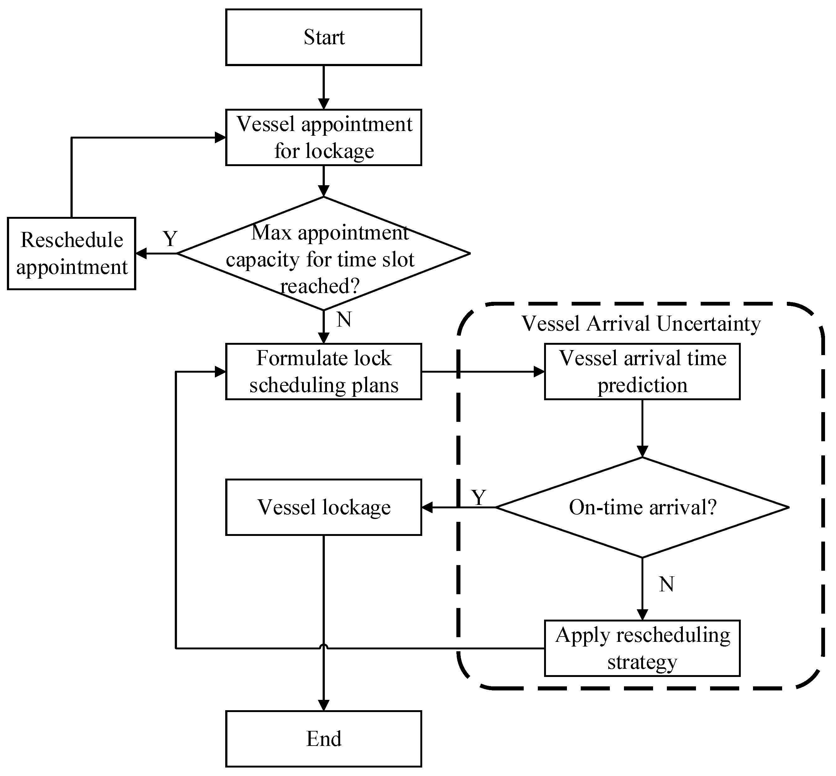
This study develops an appointment-based lock scheduling framework for inland vessels, comprising two main stages: appointment planning and execution with dynamic adjustment, as illustrated in Figure 1.

In the appointment planning stage, the system first sets capacity limits for each time slot and evaluates vessel appointment requests in real time. If the requested slot has reached its capacity, the system proactively guides the vessel to select an alternative available time slot, thereby avoiding appointment clustering and improving the overall balance of lock chamber utilization. If capacity is available, a preliminary passage plan is generated and an appointment time is assigned based on the submitted request.

In the execution and dynamic adjustment stage, a Gaussian-distribution-based neural network model is employed to probabilistically predict whether a vessel can arrive on time, outputting the expected arrival time mean and variance. If the vessel is likely to arrive as scheduled, the system executes the original appointment. Otherwise, based on predefined rescheduling rules, the system dynamically adjusts the vessel’s assigned time slot to accommodate the uncertainty and mitigate potential scheduling conflicts. Specifically, to mitigate the disruption that late-arriving vessels impose on the planned reservation schedule, we propose an arrival-triggered rescheduling strategy. For delayed vessels, the strategy reassigns them to subsequent feasible slots. Meanwhile, early-arriving vessels are actively integrated into the current schedule to dynamically fill slots vacated by delays or underutilized chamber space. Ultimately, the strategy determines the final slot allocations by jointly minimizing average waiting time, adjustment rate, and lock-chamber loss.

As illustrated in Figure 1, the decision process focuses on a single lockage slot (1.5 h) rather than the entire scheduling horizon. The system checks capacity limits specifically for the current time window. If the appointment request exceeds the limit of this 1.5-h slot, the vessel is guided to a later one. This step-by-step validation ensures that congestion is managed precisely for each lockage cycle, preventing overload in any specific period.

Furthermore, in cascade lock systems, the aforementioned gap-filling strategy provides cascading benefits. By dynamically filling vessel vacancies, it maximizes the throughput of the current hub and, to a certain extent, accelerates the dissipation of delayed queues. This flow-smoothing effect stabilizes the upstream discharge rate, thereby attenuating the propagation of arrival uncertainty and localized congestion to downstream facilities.

3.3. Arrival Time Uncertainty Quantification Model

3.3.1. Feature Vector Construction

To enable effective quantification of vessel arrival time uncertainty, a comprehensive and standardized feature vector is constructed as input to the prediction model. The feature construction process involves the following three main steps.

(1) Key feature selection

To capture the factors contributing to arrival time uncertainty, this study selects three main categories of features: temporal features, static vessel attributes, and dynamic vessel attributes. More details are shown in

Table 2. Description of selected features.

Feature Category	Feature Name	Feature Description
Temporal features	Lockage reservation timestamp	The exact time a vessel submits its request to reserve a passage slot through a lock.
	Scheduled arrival time	The estimated time of arrival at the lock is as planned by the scheduling system.
	Actual time of arrival	The clock time when the vessel actually arrives at the defined reference point (e.g., lock)
Static attributes	Vessel type	The classification of a vessel based on its primary function and design, such as a bulk carrier, container ship, etc.
	Ship length	The longitudinal dimension of a vessel from end to end.
	Ship width	The maximum transverse width of a vessel at its widest point.
	Tonnage	The total weight a vessel can safely carry.
	Priority level	The priority transit level is established according to the vessel or cargo type.
Dynamic attributes	Speed over ground	The vessel’s actual speed over the ground during its voyage.
	Traffic density	The number of vessels or congestion level in the approach channel during the voyage.
	Water flow speed	The real-time river current speed in the approach channel.

.

Temporal features: These include the scheduled arrival time and the actual time of arrival used for model training. To represent the initial condition of the scheduling plan, the vessel’s lockage reservation timestamp is also included.

Static vessel attributes: These features remain constant during navigation but significantly influence sailing performance and lock resource requirements. Key attributes include vessel type, length, beam, tonnage, and priority level.

Dynamic vessel attributes: These attributes combine the vessel’s operational state with the real-time navigational environment. Speed over ground (SOG) serves as the primary operational indicator. To address environmental complexity, the feature set couples water flow speed with traffic density.

(2) Feature quantification and normalization

For temporal features, all timestamps are converted into UNIX time format. Each value is then transformed into a relative time (in seconds) by subtracting the timestamp of midnight on the same day. This approach preserves the temporal order while effectively reducing the numerical range of the features, facilitating model training and convergence. The transformation is defined as:

$$t_{\mathrm{r}}=T_{\mathrm{t}}-T_{\mathrm{mid}}$$

(1)

where T_t denotes the original UNIX timestamp, and T_mid is the UNIX timestamp of 00:00 on the same day.

For discrete categorical features such as vessel type and priority level, this study adopts one-hot encoding [37]. This method transforms each categorical attribute into a multi-dimensional binary vector, in which only one element is set to 1 and all others are 0. For example, if there are three vessel types (bulk carrier, container ship, and chemical tanker), the category “bulk carrier” is encoded as [1, 0, 0]. This encoding technique prevents the model from performing meaningless ordinal comparisons among categories and ensures the mutual independence of categorical features, thereby enhancing model generalization and training stability.

For continuous numerical features such as vessel length, beam, tonnage, and speed over ground, the differences in units and value ranges may lead to unstable gradient updates or disproportionate feature influence during model training. To address this, Min-Max normalization [37] is applied to rescale all numerical features into the [0, 1] range. The normalization is defined as:

$$x_{norm}={\displaystyle \frac{x-x_{min}}{x_{max}-x_{min}}}$$

(2)

Here, x denotes the original feature value, while $x_{min}$ and $x_{max}$ represent the minimum and maximum values of that feature across the entire dataset.

(3) Feature vector construction

After the above processing, all features of each vessel i are integrated into a standardized feature vector ${\mathbf{x}}_i$. For a dataset containing N vessels, a final input matrix X of size N × D is formed, where D is the total number of processed feature dimensions. This matrix X serves as the final input to the subsequent deep ensemble neural network model, ensuring that the model can efficiently and accurately capture the complex relationships between features and vessel arrival time uncertainty.

3.3.2. Model Architecture

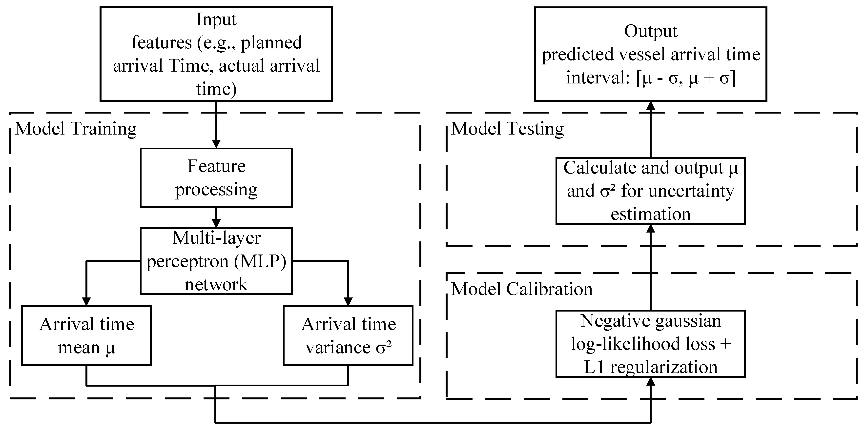
The arrival time uncertainty prediction model developed in this study adopts a deep ensemble neural network architecture, where multiple sub-networks collaborate to predict the expected value and variance of vessel arrival time, thereby characterizing its probabilistic distribution. Figure 2 illustrates the overall workflow of the model, covering key components such as feature processing, sub-network modeling, and Gaussian parameter generation, providing uncertainty modeling and quantification support for inland vessel appointment-based lock scheduling.

The first stage is the training phase, in which the model takes vessel feature vectors as input. The backbone network adopts a multi-layer perceptron (MLP) structure to perform high-dimensional feature mapping and extract key factors influencing vessel arrival time, such as channel congestion and environmental variability. To improve the model’s sensitivity to input perturbations, Monte Carlo Dropout (MC Dropout) is integrated into the backbone, randomly deactivating certain neuron connections during training. This enhances the model’s ability to capture predictive uncertainty while maintaining training stability.

To further improve robustness, the model incorporates multiple parallel sub-networks that extract intermediate features from different layers of the backbone and independently perform arrival time prediction. Their outputs are aggregated using a weighted ensemble strategy to form a unified prediction result.

Since the uncertainty in data stems from the inherent randomness of the process, it is common practice to assume the data follows a Gaussian distribution [38]. Therefore, ship arrival times are assumed to follow a Gaussian distribution with a given mean u and variance ${\sigma }^2$. The output layer is parameterized as a Gaussian distribution, jointly generating the predicted mean μ (expected arrival time) and standard deviation σ (representing uncertainty), expressed as:

$$\mu =f_u\left(x\right)$$

(3)

$${\sigma }^2=f_{{\sigma }^2}\left(x\right)$$

(4)

where x denotes the input feature vector, while $f_u$ and $f_v$ represent the independent neural network branches for predicting the mean and standard deviation, respectively.

To optimize the Gaussian distribution output, the model is trained using the negative log-likelihood (NLL) loss function, which minimizes the probabilistic distance between the predicted distribution and the actual arrival time. It is defined as follows:

$$L_{NLL}={\displaystyle \frac{1}{N}}\sum _{i=1}^N\left({\displaystyle \frac{{\left(y_i-{\mu }_i\right)}^2}{2{\sigma }_i^2}}+{\displaystyle \frac{1}{2}}ln\left(2\pi {\sigma }_i^2\right)\right)$$

(5)

where $y_i$ denotes the actual arrival time of vessel i, while ${\mu }_i$ and ${\sigma }_i$ represent the predicted mean and standard deviation, respectively. N is the total number of samples.

To improve model stability and prevent overfitting, an L1 norm regularization term is incorporated into the loss function. The resulting composite loss is defined as:

$$L=L_{NLL}+\lambda \parallel \theta {\parallel }_1$$

(6)

where λ is the regularization weight (with a value range of 0 < λ ≤ 10), and θ denotes the model parameters.

The second stage is the calibration phase, which aims to improve the stability and interpretability of the predicted variance in the Gaussian output. Due to noise in the training data and the complexity of input features, the model’s initial variance predictions may deviate from reality, resulting in distorted uncertainty intervals and reduced reliability of the predictive distribution. To address this issue, an auxiliary loss term is introduced to regularize the predicted variance and suppress its undesired divergence. This approach enhances the numerical stability and semantic consistency of variance estimation while preserving sensitivity to input perturbations, thereby improving the overall reliability of the predicted distribution. The auxiliary loss term is defined as follows:

$$L_{\sigma }={\displaystyle \frac{1}{N}}\sum _{i=1}^N\hspace{0.33em}\left|{\sigma }_i-{\sigma }_{ref}\right|$$

(7)

where ${\sigma }_{\mathrm{r}\mathrm{e}\mathrm{f}}$ denotes the reference variance, which serves to constrain the model output and ensure that the predicted variance remains within a reasonable range.

The third stage is the testing phase, during which the model uses the trained and calibrated parameters to generate the final arrival time prediction and its corresponding uncertainty interval based on the input feature vector. The prediction follows a Gaussian distribution N(μ, σ²), where μ denotes the most likely arrival time (i.e., the mean), and σ represents the standard deviation. The uncertainty interval is defined as [μ−ασ, μ+ασ], where α is a confidence factor. This interval provides a quantitative boundary for uncertainty, enabling the scheduling system to dynamically adjust appointment windows and improve both responsiveness and robustness.

3.4. Appointment-Based Lock Scheduling Model for Inland Vessels Under Arrival Time Uncertainty

3.4.1. Modeling Assumptions

To ensure the feasibility and practical applicability of the model, several rational assumptions and simplifications are made regarding the scheduling scenario and operational rules. These include the following:

(1)

Appointment Constraint Assumption: To guarantee the proactiveness and controllability of the scheduling system, it is assumed that all vessels must complete appointment registration at least one day in advance. Vessels without appointments are excluded from the current scheduling model and are not considered in resource allocation or queuing decisions.

(2)

Missed Appointment Handling: The rescheduling mechanism in this model only applies to cases of delayed arrival, where vessels arrive later than their reserved time slots but are still within the lock waiting area. Vessels that cancel their appointment or fail to arrive entirely are removed from the scheduling plan and are not included in rescheduling or resource reallocation.

(3)

Chamber Allocation Simplification: To ensure computational tractability while maintaining spatial accuracy, vessels are geometrically represented as rigid rectangles based on their maximum length and width. A lockage allocation is considered physically feasible if these rectangular models can be packed within the lock chamber boundaries without any overlapping.

3.4.2. Appointment-Based Scheduling Model

Under the condition of uncertain vessel arrival times, lock scheduling must possess dynamic adaptability to accommodate fluctuations in actual traffic flow. To achieve this, operators may adjust appointment quotas and rescheduling policies in real time, guiding vessels to distribute more evenly across available time slots and smoothing the overall arrival pattern.

The core objective of scheduling is to jointly minimize three key performance indicators: average vessel waiting time, appointment adjustment ratio, and lock resource loss rate. Based on this, a multi-objective optimization model is formulated as follows:

$$min{Z}_1={\displaystyle \frac{{\sum }_{n=1}^N{\sum }_{i=1}^I{W}_{ni}{\lambda }_{ni}}{{\sum }_{n=1}^N{\sum }_{i=1}^I{\lambda }_{ni}}}$$

(8)

$$min{Z}_2={\displaystyle \frac{{\sum }_{n=1}^N\hspace{0.33em}{\sum }_{i=1}^I\hspace{0.33em}max\left\{A_{ni}-B_{ni}+x_{ni}-y_{ni},x_{ni}\right\}}{{\sum }_{n=1}^N\hspace{0.33em}{\sum }_{i=1}^I\hspace{0.33em}{A}_{ni}}}$$

(9)

$$min{Z}_3={\displaystyle \frac{{\sum }_{n=1}^N\left(S_n-{\sum }_{i=1}^I{L}_{ni}\right)}{{\sum }_{n=1}^N{S}_n}}$$

(10)

$$s.t.\left\{\begin{array}{cc}0<{\displaystyle {\sum }_{n=1}^N{\displaystyle {\sum }_{i=1}^I{\lambda }_{ni}\le {\displaystyle {\sum }_{n=1}^N{\displaystyle {\sum }_{i=1}^I{A}_{ni}}}}}\hfill & \hfill \hspace{1em}\hspace{1em}\hspace{1em}(11)\\ 0<y_{ni}\le A_{ni}+x_{ni}\hfill & \hfill \hspace{1em}\hspace{1em}\hspace{1em}(12)\\ 0<{\lambda }_{ni}\le y_{ni}\hfill & \hfill \hspace{1em}\hspace{1em}\hspace{1em}(13)\\ u_i-F^{-1}{\sigma }_i\le T{p}_i\le u_i+F^{-1}{\sigma }_i\hfill & \hfill \hspace{1em}\hspace{1em}\hspace{1em}(14)\\ 0\le x_{ni}\le \alpha ·(A_{ni}+x_{ni})\hfill & \hfill \hspace{1em}\hspace{1em}\hspace{1em}(15)\\ {\displaystyle {\sum }_{i}sare{a}_i\le Larea}\hfill & \hfill \hspace{1em}\hspace{1em}\hspace{1em}(16)\\ {\displaystyle \sum _{k=1}^K{\displaystyle \sum _{i=1}^m{L}_{ik}}}⩽L\hfill & \hfill \hspace{1em}\hspace{1em}\hspace{1em}(17)\\ {\displaystyle \sum _{k=1}^K{\displaystyle \sum _{i=1}^m{W}_{ik}}}⩽W\hfill & \hfill \hspace{1em}(18)\\ L_{ik}=l_{ik}+l_{\mathrm{safe}}\hfill & \hfill \hspace{1em}\hspace{1em}\hspace{1em}(19)\\ W_{ik}=w_{ik}+w_{\mathrm{safe}}\hfill & \hfill \hspace{1em}\hspace{1em}\hspace{1em}(20)\end{array}\right.$$

where objective function (8) minimizes the average waiting time of vessels within the reservation horizon. $Z_1$ denotes the objective function of average vessel waiting time. N is the total number of vessels. I is the total number of reservation attempts. $W_{ni}$ is the average waiting time of vessel i for the i-th appointment period on day n. ${\lambda }_{ni}$ is the actual number of vessels arriving during the i-th appointment on day n. Objective function (9) minimizes the vessel arrival adjustment ratio within the reservation horizon. $Z_2$ represents the objective function of vessel arrival adjustment ratio. $A_{ni}$ is the number of vessel arrivals under the originally declared system for the i-th reservation on day n, $B_{ni}$ is the vessel number of missed appointment for the i-th reservation on day n, $x_{ni}$ represents the number of rescheduled vessels for the i-th appointment period on day n, and $y_{ni}$ is the assigned appointment quota for that time slot. Objective function (10) minimizes the lock chamber loss rate within the reservation horizon. Here, $Z_3$ denotes the objective function of lock chamber loss rate. $S_n$ is the utilized lock chamber area on day n, and $L_{ni}$ is the area loss due to no-shows during the i-th appointment on day n.

The constraints are defined as follows: Constraint (11) ensures scheduling feasibility by requiring that the total number of vessels scheduled for passage does not exceed the total number of vessels that have actually arrived. Constraint (12) ensures that the appointment quota for each time slot is sufficient to accommodate both normally arriving vessels and d vessels. Constraint (13) dictates that the number of vessels scheduled to pass in a given time slot cannot exceed the assigned quota for that slot. Constraint (14) mandates that the effective passage time ($T{p}_i$) for a vessel must fall within its predicted arrival time confidence interval, defined by the mean ($u_i$) and standard deviation (${\sigma }_i$). Constraint (15) limits the maximum allowable rescheduling rate, denoted by α. Constraint (16) ensures that the total occupied area of vessels in a single lock operation does not exceed the chamber’s capacity. Here, ${sarea}_i$ is the lock chamber area occupied by vessel i, and Larea is the total lock chamber area. Constraint (17)–(20) ensures that any two vessels are separated by a safe distance in at least one spatial direction, and the sum of the safety zone dimensions of the transiting vessels must be less than the dimensions of the lock chamber.$L_{ik},W_{ik}$ represents the usable length and width of the lock chamber, respectively. $L_{ik},W_{ik}$ represents the length and width of the safety zone for the i-th vessel entering the lock chamber during the k-th time period, respectively. $l_{ik},w_{ik}$ represents the length and width of the i-th vessel entering the lock chamber during the k-th time period, respectively. $l_{safe},w_{safe}$ represents the length and width of the safe distance for vessel navigation, respectively.

The mathematical symbols of the appointment-based lock scheduling model are described in

Table 3. The mathematical symbols of model.

Symbols	Explanations
$Z_1$	Average ship waiting time objective function
$Z_2$	Ship arrival adjustment rate objective function
$Z_3$	Lock chamber loss rate objective function
N	Total number of ships
I	Total number of ship appointment attempts
$W_{ni}$	Average ship waiting time for the i-th appointment period on day n
${\lambda }_{ni}$	Actual number of ship arrivals in the i-th appointment period on day n
$A_{ni}$	Number of vessel arrivals under the declared system for the i-th appointment period on day n
$B_{ni}$	vessel number of missed appointment for the i-th reservation on day n
$x_{ni}$	Number of rescheduled vessels for the i-th appointment period on day n
$y_{ni}$	Assigned appointment quota for the i-th appointment period on day n
$S_n$	Utilization area of the lock chamber on day n
$L_{ni}$	Lock chamber area occupied by missed appointment of ships for i-th appointment period on day n
${Tp}_i$	Passage time for vessels under the i-th ship appointment schedule
$F^{-1}$	Confidence probability under ship appointment schedule
$u_i$	Mean of arrival time under the i-th ship appointment schedule
${\sigma }_i$	Standard deviation of arrival time under the i-th ship appointment schedule
α	Maximum allowable rescheduling rate
${sarea}_i$	Utilization area of lock chamber occupied by vessel i
Larea	Total area of the lock chamber
L, W	Usable length and width of the lock chamber, respectively
$L_{ik},W_{ik}$	The length and width of the safety zone for the i-th vessel entering the lock chamber during the k-th time period, respectively
$l_{ik},w_{ik}$	The length and width of the i-th vessel entering the lock chamber during the k-th time period, respectively
$l_{safe},w_{safe}$	The length and width of the safe distance for vessel navigation, respectively

.

3.5. Improved Optimization Algorithm

3.5.1. Hybrid VNS-NSGA-II Algorithm

NSGA-II (Non-dominated Sorting Genetic Algorithm II) is a classical multi-objective evolutionary algorithm that has been widely applied to solving multi-objective optimization problems [39]. By incorporating fast non-dominated sorting, crowding distance comparison, and elitism, NSGA-II effectively approximates the Pareto-optimal front. However, when dealing with large-scale and constraint-rich combinatorial problems, it often suffers from weak local search capability, premature convergence, and insufficient global exploration [39], which can limit both solution diversity and optimality.

To enhance search robustness and the ability to escape local optima, this study integrates the Variable Neighborhood Search (VNS) strategy into the NSGA-II framework. VNS is a metaheuristic that dynamically switches between different neighborhood structures, enabling wider exploration and more efficient local refinement. The resulting hybrid VNS-NSGA-II algorithm is tailored to the appointment-based lock scheduling problem for inland vessels, with the goal of improving solution quality and the uniformity of the Pareto front.

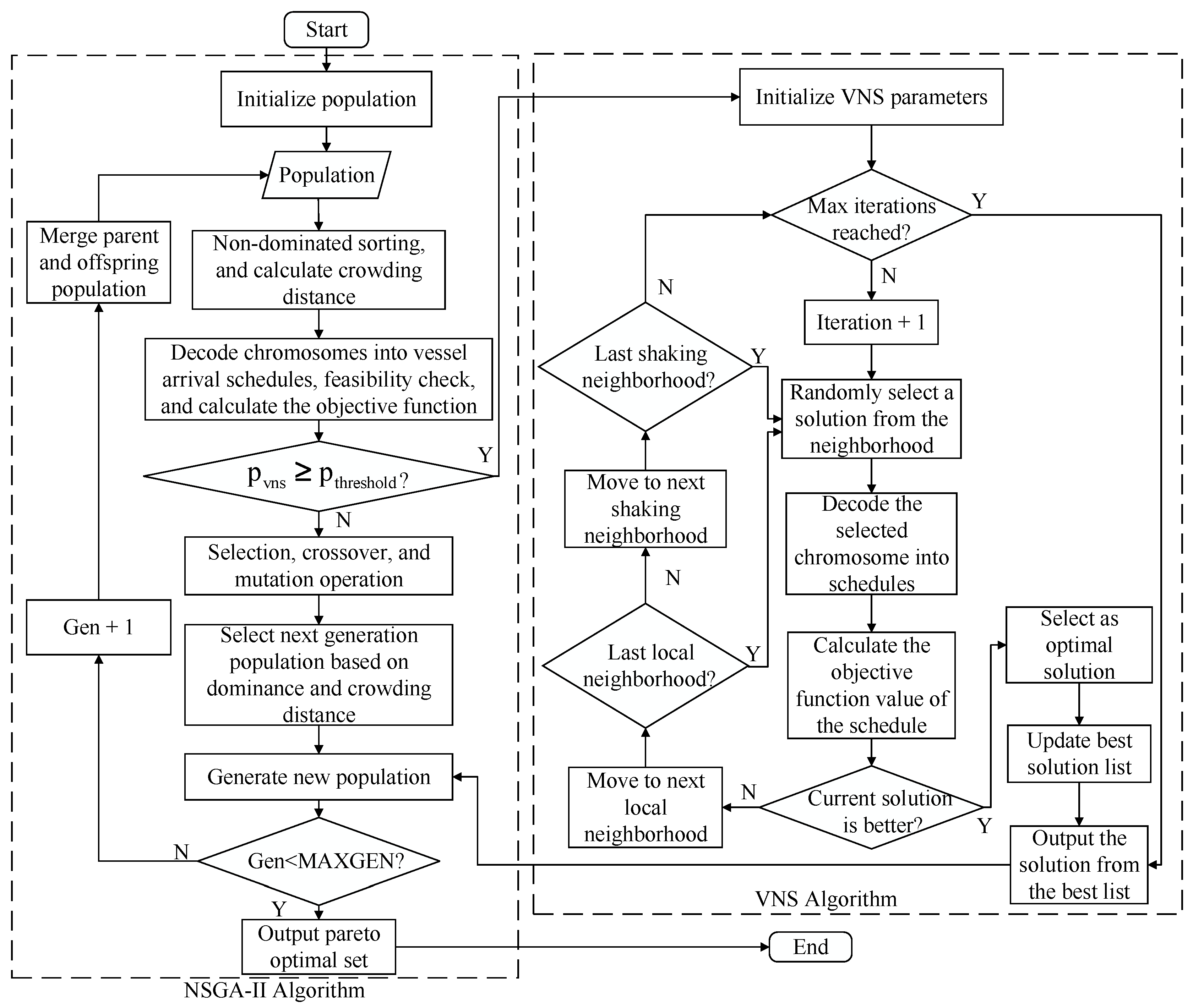
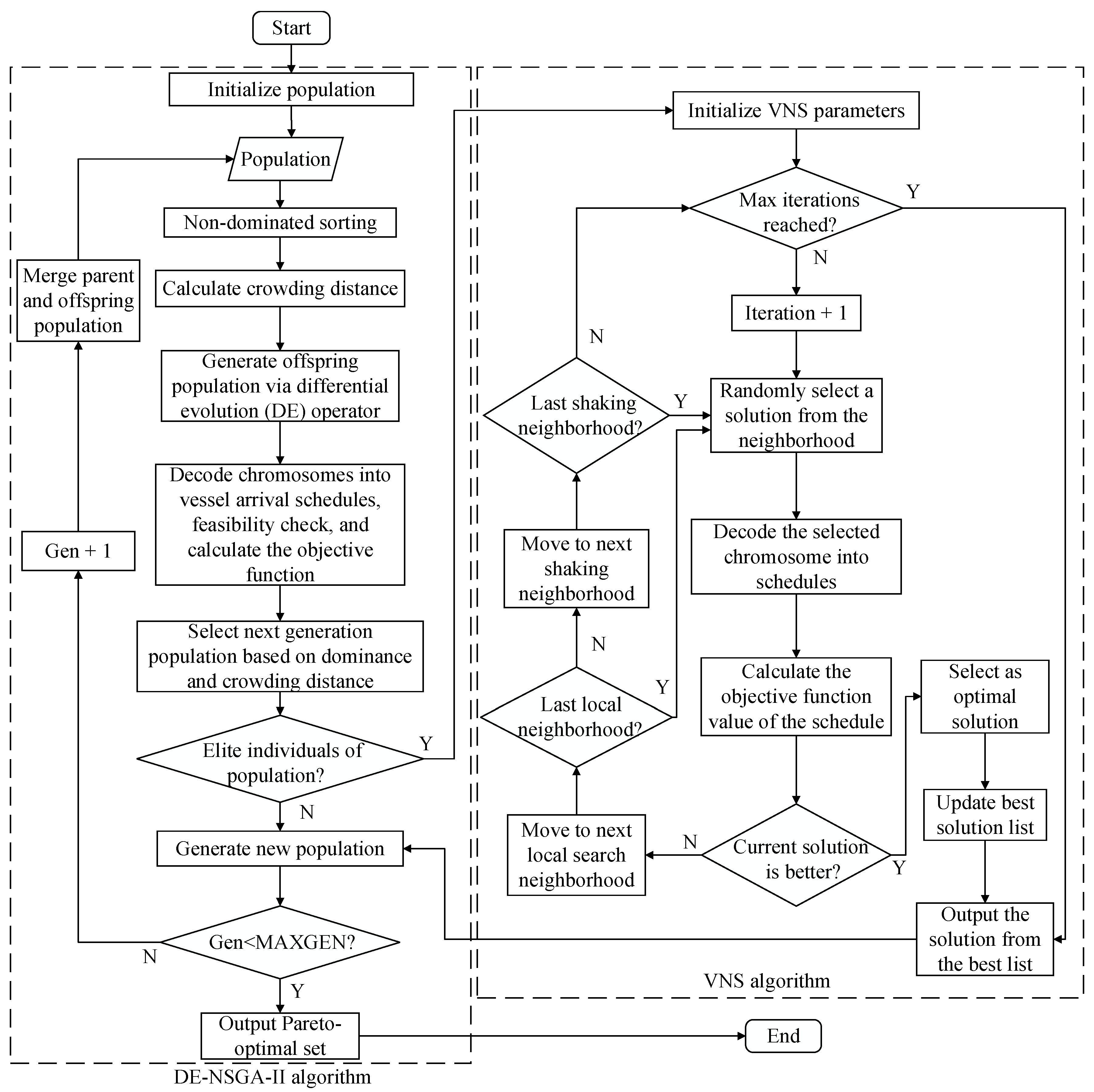
The overall workflow of the proposed hybrid VNS–NSGA-II algorithm is illustrated in Figure 3. NSGA-II serves as the main framework, within which a VNS module is embedded to achieve coordinated global and local search. The algorithm starts by initializing a population of candidate solutions, each representing a feasible appointment schedule. Through fast non-dominated sorting and crowding distance comparison, high-quality individuals are selected.

In each iteration, NSGA-II performs crossover and mutation to generate offspring, which are combined with the parent population for sorting and selection. If the maximum number of generations (MAXGEN) is not reached, the algorithm enters the VNS module when the selection probability of each solution for VNS $p_{vns}$ exceeds probability threshold $p_{threshold}$, where it dynamically switches among perturbation neighborhoods ${SD}_{\mathsf{\Theta }}$(Θ = 1, 2, 3) and local search structures ${LS}_{\mathsf{\varpi }}$(ϖ = 1, 2, 3). Perturbations are applied to escape local optima, followed by local refinement within each neighborhood to enhance solution diversity and quality.

The improved solutions are then fed back into the NSGA-II population for the next generation. This process repeats until the termination condition is met, ultimately yielding a high-quality Pareto front that provides a robust and balanced scheduling solution for inland vessel lock operations.

3.5.2. DE-VNS-NSGA-II Algorithm

To enhance global search capability and convergence efficiency, and to address the tendency of traditional NSGA-II to fall into local optima, this study integrates a Differential Evolution (DE) mechanism into the VNS-NSGA-II framework, forming a hybrid multi-objective algorithm termed DE-VNS-NSGA-II. In this approach, DE serves as the main evolutionary engine to replace conventional crossover and mutation, while VNS provides local search and NSGA-II ensures elite selection, yielding a complementary and synergistic optimization framework. The procedure of DE-VNS-NSGA-II is shown in Figure 4.

The DE operator in this algorithm consists of three basic operations: mutation, crossover, and selection. To balance convergence speed and population diversity, a “DE/current-to-pbest” mutation strategy is adopted, which combines fast convergence with diversity preservation. This strategy guides the search direction by exploiting information from superior individuals within the current population. For each target vector $z_{i,g}$ in the current population, the corresponding mutant vector $m_{i,g}$ is generated as follows:

$$m_{i,g}=z_{i,g}+S·\left(z_{\mathit{elite},g}^q-z_{i,g}\right)+S·\left(z_{r1,g}-z_{r2,g}\right)$$

(21)

Here, $z_{i,g}$ denotes the current individual in generation g. $z_{\mathrm{elite},g}^q$ is an elite vector randomly selected from the top individuals of the current population, and q is a parameter in the interval (0, 1] that determines the greediness of the mutation strategy. $z_{r1,g}$ and $z_{r2,g}$ are two distinct individuals randomly chosen from the population, whose difference vector is used to generate perturbations; S is a fixed scaling factor. In the classical DE algorithm, the control parameters are typically kept constant throughout the entire evolutionary process.

After generating the mutant vector $m_{i,g}$, a binomial crossover is applied to construct the trial vector $w_{j,i,g}$, where the elements of the mutant and target vectors are recombined with a given probability as follows:

$$w_{j,i,g}=\left\{\begin{array}{ll}{m}_{j,i,g}& {\mathrm{rand}}_j\le CP \mathrm{or} j=j_{\mathrm{rand}}\\ z_{j,i,g}& \mathrm{otherwise}\end{array}\right.$$

(22)

where j denotes the dimension index of the vector. CP is the fixed crossover probability, and $j_{\mathrm{rand}}$ represents a randomly generated dimensional index. This ensures the trial vector inherits at least one dimension from the mutant vector, thereby guaranteeing effective information exchange. Finally, a one-to-one greedy selection strategy is applied between the trial vector $w_{i,g}$ and its corresponding target vector $z_{i,g}$, with the superior individual retained for the next generation. For a minimization problem, the selection process can be expressed as follows:

$$z_{i,g+1}=\left\{\begin{array}{ll}{w}_{i,g}& f\left(w_{i,g}\right)\le f\left(z_{i,g}\right)\\ z_{i,g}& f\left(w_{i,g}\right)>f\left(z_{i,g}\right)\end{array}\right.$$

(23)

where f (·) denotes the objective function value. These three operations—mutation, crossover, and selection—collectively constitute the complete Differential Evolution (DE) operator. This operator is embedded into the iterative process of the hybrid DE-VNS-NSGA-II algorithm, serving as its core global search engine. It works synergistically with the local refinement capability of VNS and the elite preservation mechanism of NSGA-II to jointly drive the population to evolve efficiently and stably towards the Pareto-optimal front.

4. Case Study

4.1. Data Instances

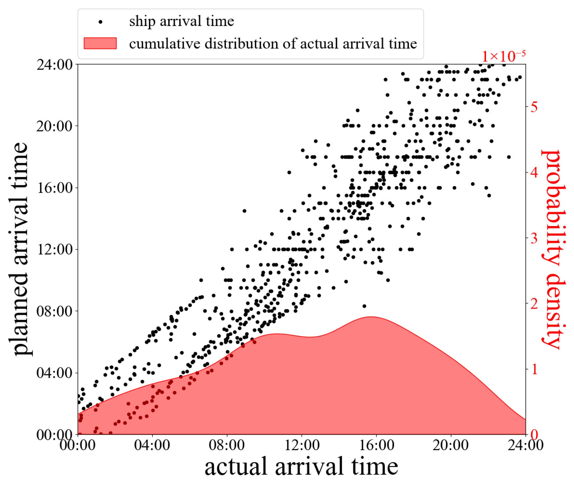
The experimental data used in this study were derived from 15 consecutive days of vessel lock passage records at a certain inland waterway transportation hub. To visually illustrate the uncertainty in vessel arrival times, this paper compares the planned arrival times with the actual arrival times and plots a scatter diagram as shown in Figure 5. The horizontal axis represents the planned arrival time, while the vertical axis indicates the corresponding actual arrival time.

As shown in Figure 5, most data points cluster near the diagonal line, indicating a strong positive correlation between the two variables. However, a number of scattered points deviate significantly from the diagonal, forming a broad distribution band that visually reveals substantial fluctuations in actual arrival times. Any scheduling strategy relying on deterministic planned times risks failure during actual operation. This uncertainty constitutes the key challenge addressed by this study.

To further reveal the temporal patterns of vessel arrivals, a kernel density estimation (KDE) curve is superimposed at the bottom of the figure. This curve illustrates the probability density distribution of the actual arrival times. The shape of the density curve indicates that vessel arrivals are not uniformly distributed but exhibit pronounced peaks during specific periods, particularly around 15:00–18:00. This “tidal phenomenon” demonstrates the practical necessity of implementing lock reservation and scheduling mechanisms to achieve peak shaving and valley filling.

4.2. Parameter Tuning

The DE-VNS-NSGA-II algorithm contains several critical parameters: Population sizes, NP; Iterations of DE and NSGA-II algorithm; $Iter\_NSDE$; Crossover probability, Pc; Mutation probability, Pm; Scaling factor, Sf; Max neighbors, kmax; Max iterations of the VNS algorithm, $MaxIter\_VNS$; Interval parameter of frequency interaction between algorithms, K.

The best parameter combination of the algorithm is determined through multiple orthogonal simulation experiments [40].

Table 4. Levels of the parameters for DE-VNS-NSGA-II Algorithm.

Parameter	Parameter Level
	1	2	3	4	5
NP	80	90	100	110	120
$Iter\_NSDE$	100	150	200	250	300
Pc	0.7	0.75	0.8	0.85	0.9
Pm	0.05	0.1	0.15	0.2	0.25
Sf	0.2	0.3	0.4	0.5	0.6
kmax	1	2	3	4	5
$MaxIter\_VNS$	500	1000	1500	2000	2500
K	10	30	50	70	90

shows that each parameter is treated as a factor varying at five different levels. To ensure the credibility of the experiment, the DE-VNS-NSGA-II algorithm performs 20 independent repeated experiments on each combination at the same time limit. Meanwhile, the average HV values are collected as the response variable. HV metric [41] is calculated as follows:

$$\mathrm{HV}=\mathrm{volume}\left(U_{z=1}^{W_{\max }}\left[f_1\left({\omega }_z\right),r_1\right]\times \dots \times \left[f_K\left({\omega }_z\right),r_K\right]\right)$$

(24)

where $\{r_1,r_2,\dots ,r_k\}$ represents the referenced point for all the objectives. Obviously, a greater HV value represents a better combination.

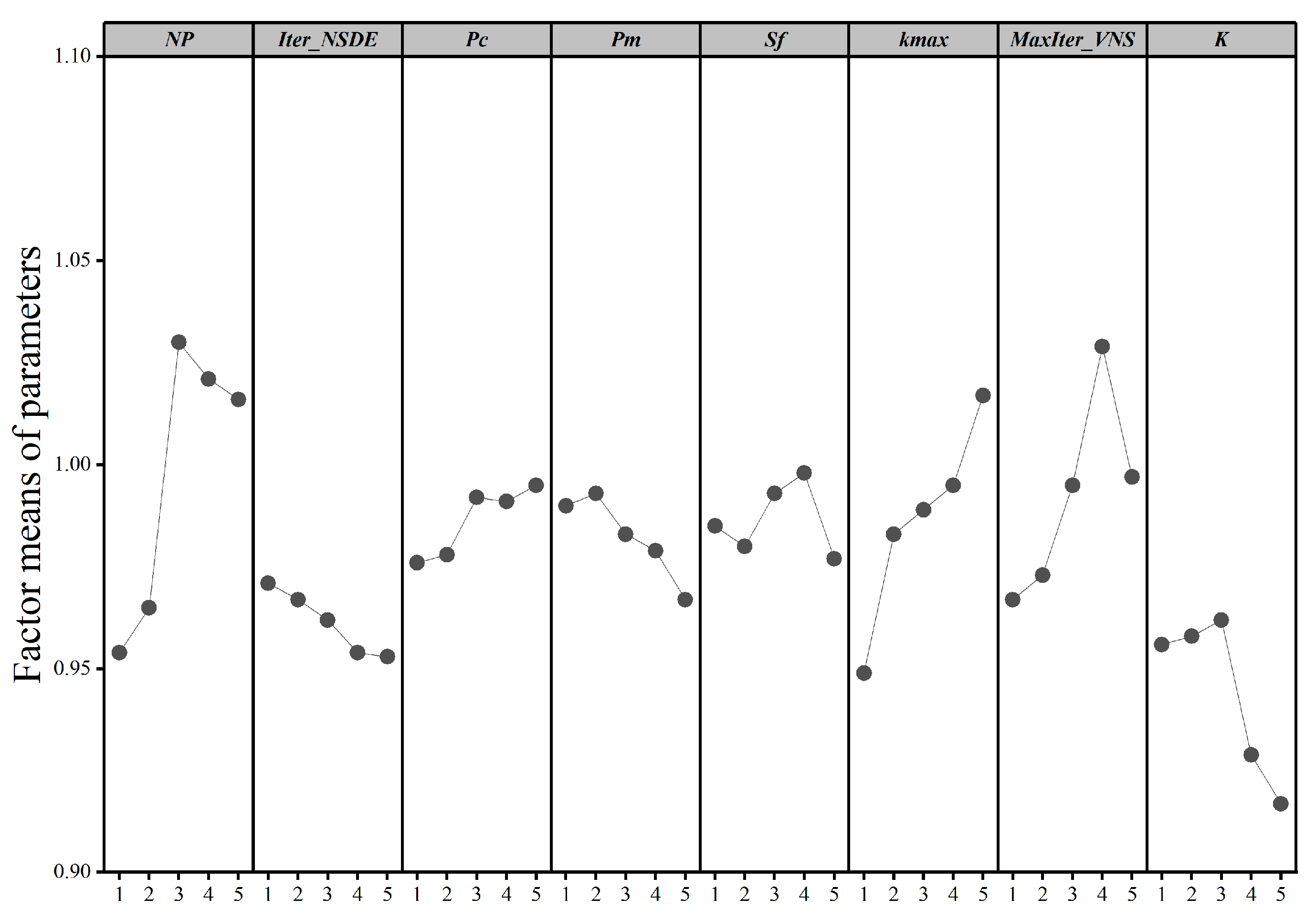
By conducting a sensitivity analysis and comparing the results of the main effect in Figure 6, the optimal parameter combination sets of the DE-VNS-NSGA-II algorithm are as follows: $NP=100$, $Iter\_NSDE=200$, $Pc=0.9$, $Pm=0.1$, $Sf=0.5$, $kmax=5$, $MaxIter\_VNS=1000$, $k=50$.

We also adopt a Taguchi analysis method for the other four competitive algorithms (i.e., NSGA-II, VNS-NSGA-II, GSAA-RL [42] and ADEA-KC [43]). Due to the reason of space limitations, we only provide the values of parameters after tuning in

Table 5. The parameters for the competitive algorithms.

Algorithms	Parameters
NSGA-II	$NP=100$, $Ite{r}_{NSGA2}=200$, $Pc=0.9$, $Pm=0.2$
VNS-NSGA-II	$NP=100$, $Iter\_NSGA2=200$, $Pc=0.8$, $Pm=0.2$, $kmax=5$, $MaxIter\_VNS=1000$, $Pvns=0.1$
GSAA-RL [42]	$NP=100$, $Maxgen=400,GGAP=0.9$, $T_0=2,R=0.9$, $\alpha =0.6, \gamma =0.65, \epsilon =0.85$
ADEA-KC [43]	$NP=120,N_{Cluster}=6,Ite{r}_{kmeans}=15,Maxgen=200,\alpha =0.75,\gamma =0.6,\epsilon =0.7$

Notes: $Iter\_NSGA2$: Iterations of NSGA-II algorithm; $Maxgen$: Max generations; $GGAP$: Selection probability; $T_0$: Initial temperature; $R$: Cooling factor; $\alpha$: Learning rate; $\gamma$: Discount rate; $\epsilon$: Greed rate; $N_{Cluster}$: Cluster number; $Ite{r}_{kmeans}$: Iterations of K-means algorithm.

.

4.3. Analysis of Uncertainty Intervals of Vessel Arrival Times

4.3.1. Prediction of Uncertainty Intervals of Vessel Arrival Times

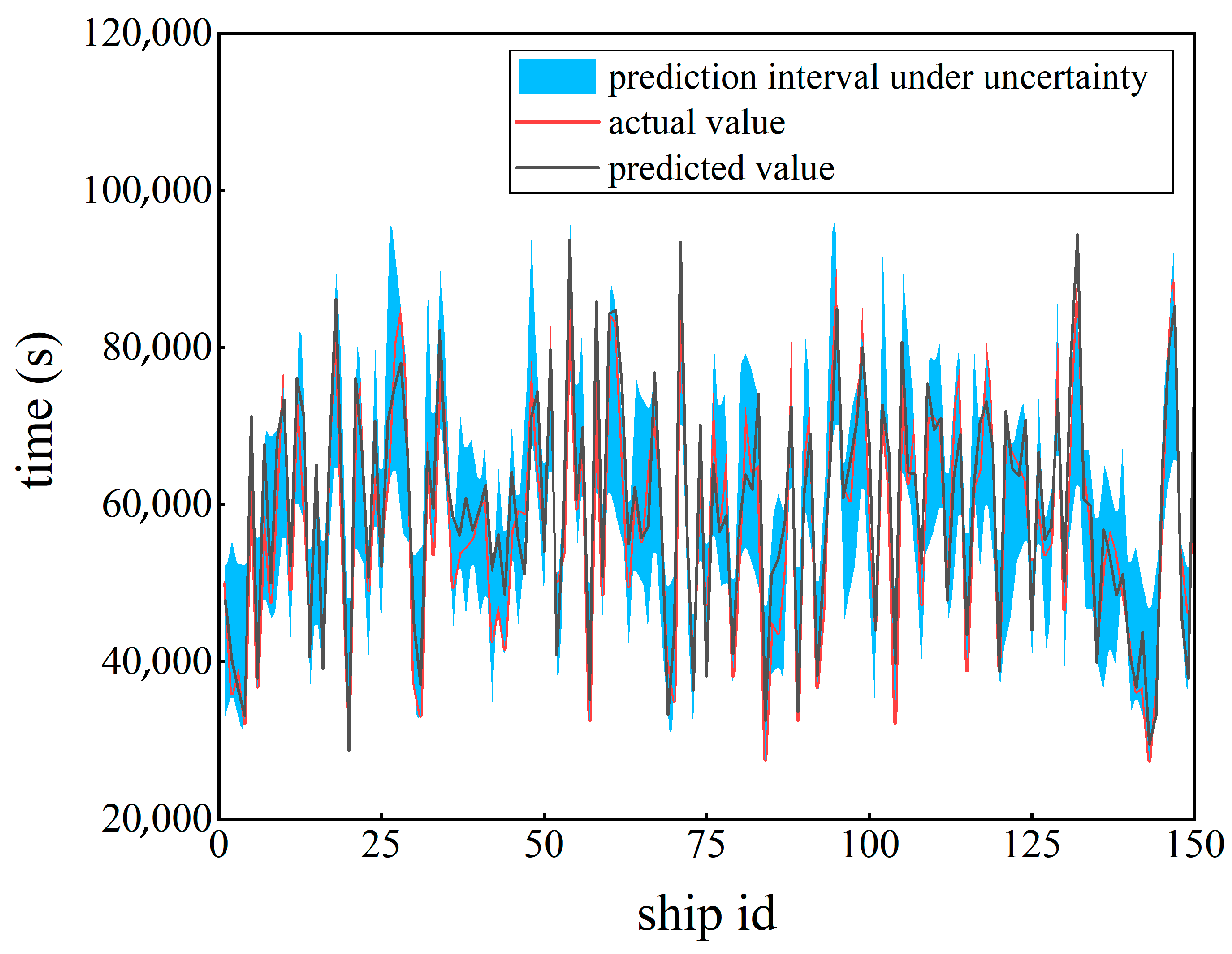
Figure 7 illustrates the quantified uncertainty of vessel arrival time predictions. The horizontal axis corresponds to vessel IDs, while the vertical axis denotes the arrival time. The red curve represents the actual arrival times, the black curve indicates the predicted values, and the blue shaded region marks the model’s predicted uncertainty intervals. These intervals reflect the model’s confidence: wider intervals imply higher uncertainty and lower reliability, whereas narrower intervals suggest greater confidence in the predictions.

As shown in Figure 7, all actual arrival times lie within the predicted uncertainty intervals. This finding confirms the effectiveness of the proposed uncertainty quantification method for vessel arrival time prediction. It demonstrates the model’s ability to reliably capture the range of prediction uncertainty, thereby providing a robust data foundation for subsequent uncertainty-aware vessel scheduling optimization.

4.3.2. Validation of Uncertainty Intervals of Vessel Arrival Times

To validate the uncertainty intervals of vessel arrival times, we consider model outputs that consist of the predicted arrival times together with their corresponding uncertainty intervals. This setup provides a comprehensive view of both accuracy and confidence. Given that inland waterway shipping is affected by numerous uncontrollable factors, perfectly precise predictions are infeasible; accordingly, we adopt a 90% confidence level (significance level of 0.1) as the target coverage for the intervals.

The accuracy of the predicted arrival times is evaluated using Mean Absolute Error (MAE), Root Mean Square Error (RMSE), and Mean Absolute Percentage Error (MAPE) [44], while interval reliability is assessed by the empirical coverage under the 90% target. The corresponding formulas are given as follows:

$$MAE={\displaystyle \frac{1}{N}}\sum _{i=1}^N\hspace{0.33em}\left|\left(y_i-{\widehat{y}}_i\right)\right|$$

(25)

$$RMSE=\sqrt{{\displaystyle \frac{1}{N}}\sum _{i=1}^N\hspace{0.33em}{\left(y_i-{\widehat{y}}_i\right)}^2}$$

(26)

$$MAPE={\displaystyle \frac{1}{N}}\sum _{i=1}^N\hspace{0.33em}{\displaystyle \frac{\left|{\widehat{y}}_i-y_i\right|}{\left|y_i\right|}}$$

(27)

where $y_i$ denotes the true value of the i-th sample. ${\widehat{y}}_i$ is the predicted value of the i-th sample. N represents the number of sample data points for prediction.

To validate the reliability and practical interpretability of the prediction intervals for vessel arrival time, this study introduces two commonly used evaluation metrics: Prediction Interval Coverage Probability (PICP) and Mean Prediction Interval Width (MPIW) [45].

PICP quantifies the proportion of actual arrival times falling within the predicted ETA intervals at a given confidence level. Ideally, at a 90% confidence level, about 90% of true values should be contained. A significantly lower PICP indicates overestimated model confidence. Its mathematical expression is:

$$PICP={\displaystyle \frac{1}{N}}\sum _{i=1}^N\hspace{0.33em}\mathbb{I}\left(y_i\in \left[{\widehat{y}}_{i,L},{\widehat{y}}_{i,U}\right]\right)$$

(28)

where N denotes the total number of samples. y_i is the true observed value of the i-th sample. ${\widehat{y}}_{i,L}$ and ${\widehat{y}}_{i,U}$ represent the lower and upper bounds of the predicted interval for the i-th sample, respectively. $\mathbb{I}\left(·\right)$ is the indicator function, which equals 1 if the condition inside the parentheses is satisfied and 0 otherwise.

MPIW is defined as the average width of all prediction intervals, reflecting the compactness of the intervals. A smaller MPIW indicates a more precise characterization of uncertainty and greater practical utility. In practice, it is important to balance PICP and MPIW to avoid excessively wide intervals that reduce usability or overly narrow intervals that fail to provide sufficient coverage. The mathematical expression of MPIW is:

$$MPIW={\displaystyle \frac{1}{N}}\sum _{i=1}^N\hspace{0.33em}\left({\widehat{y}}_{i,U}-{\widehat{y}}_{i,L}\right)$$

(29)

To assess the performance of uncertainty interval estimation, this study evaluates the proposed model (M3) against two representative uncertainty forecasting methods using five metrics. These two reference methods are: M1 (Quantile Regression Model) [37]: avoids specific distributional assumptions and directly models conditional quantiles; M2 (Monte Carlo Dropout Model) [46]: approximates Bayesian inference by applying Dropout during both training and inference.

As shown in

Table 6. Comparison of Uncertainty Interval Validation for Vessel Arrival Times among M1, M2, and M3.

Metric	M1	M2	M3
MAE	10.76	10.49	10.39
RMSE	13.45	12.89	12.83
MAPE	13.64	12.88	12.57
PICP	85.32	80.69	93.45
MPIW	29.78	25.93	22.57

, the proposed model (M3) delivers superior performance in both arrival time prediction and uncertainty quantification. For arrival time prediction, M3 achieves the lowest errors across three key metrics: a Mean Absolute Error (MAE) of 10.39, a Root Mean Square Error (RMSE) of 12.83, and a Mean Absolute Percentage Error (MAPE) of 12.57%. These results consistently surpass those of the Quantile Regression model (M1) and the MC Dropout model (M2), underscoring the higher predictive accuracy of M3. In terms of uncertainty quantification, M3 attains a Prediction Interval Coverage Probability (PICP) of 93.45%, compared with 85.32% for M1 and 80.69% for M2, demonstrating its stronger interval reliability. More importantly, while ensuring sufficient coverage, M3 achieves the narrowest Mean Prediction Interval Width (MPIW) of 22.57, highlighting its superior interval compactness and more precise representation of uncertainty.

4.4. Results of Optimization in Vessel Lockage Appointment Scheduling

Using the Three Gorges Navigation Hub on the Yangtze River as the case study, vessels with lockage demands over a consecutive three-day period were selected to construct the data sample set (see

Table 7. Ship dataset for lock schedule.

Ship ID	Application Time for Appointment	Estimated Arrival Time	Ship Type	Ship Width (m)	Ship Length (m)	Ship Tonnage (t)	Ship Priority	Ship Speed (kn)
1	2024-01-04 00:24:00	2024-01-08 01:07:48	bulk carrier	17.01	81.76	7842.68	1	6
2	2024-01-04 21:47:00	2024-01-08 01:35:16	bulk carrier	17.35	132.77	6974.18	1	7
3	2024-01-03 15:13:00	2024-01-08 03:56:03	bulk carrier	15.77	101.78	6188.76	1	7
4	2024-01-07 22:25:00	2024-01-08 03:56:57	container ship	16.93	109.3	1389.82	6	4
5	2024-01-01 14:08:00	2024-01-08 04:03:35	Ro-Ro ship	16.25	105.1	6714.37	1	5
…	…	…	…	…	…	…	…	…
140	2024-01-10 17:31:00	2024-01-10 20:40:41	bulk carrier	15.41	83.08	4884.99	1	7
141	2024-01-10 16:18:00	2024-01-10 20:43:33	bulk carrier	15.11	84.62	5298.74	1	5
142	2024-01-10 15:41:00	2024-01-10 21:12:57	bulk carrier	13	86.66	4410.4	1	4
143	2024-01-05 03:40:00	2024-01-10 21:39:20	bulk carrier	18.16	93.92	6058.44	1	6

). The entire period was discretized into 48 scheduling sessions of 1.5 h each, within which approximately 143 vessels submitted lockage requests. It should be emphasized that the vessel priority indicated in Table 7 refers to the preferential lockage rights granted to vessels due to the time-sensitivity of their cargo. In accordance with the regulations of the Three Gorges Ship Lock, passenger vessels and container ships, for example, are entitled to priority passage.

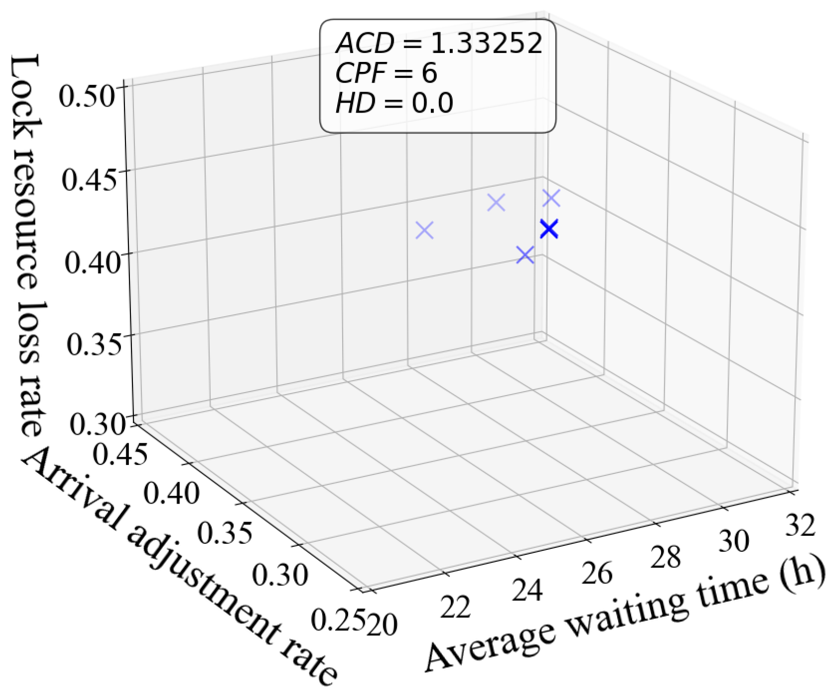
Figure 8 shows the Pareto front of scheduling solutions obtained by the NSGA-II algorithm under uncertain vessel arrival times. The value of the average crowding distance (ACD), the cardinality of the Pareto front (CPF), and the Hausdorff distance (HD) are 1.33252, 6, 0, respectively. Using the Pareto front of the NSGA-II algorithm as the baseline reference, an HD equal to 0 demonstrates that the proposed algorithm has achieved the exact same non-dominated solutions. The front is moderately dispersed, with most solutions concentrated at intermediate levels of waiting time and imbalance, indicating a basic capacity for multi-objective trade-offs, though stability could be improved.

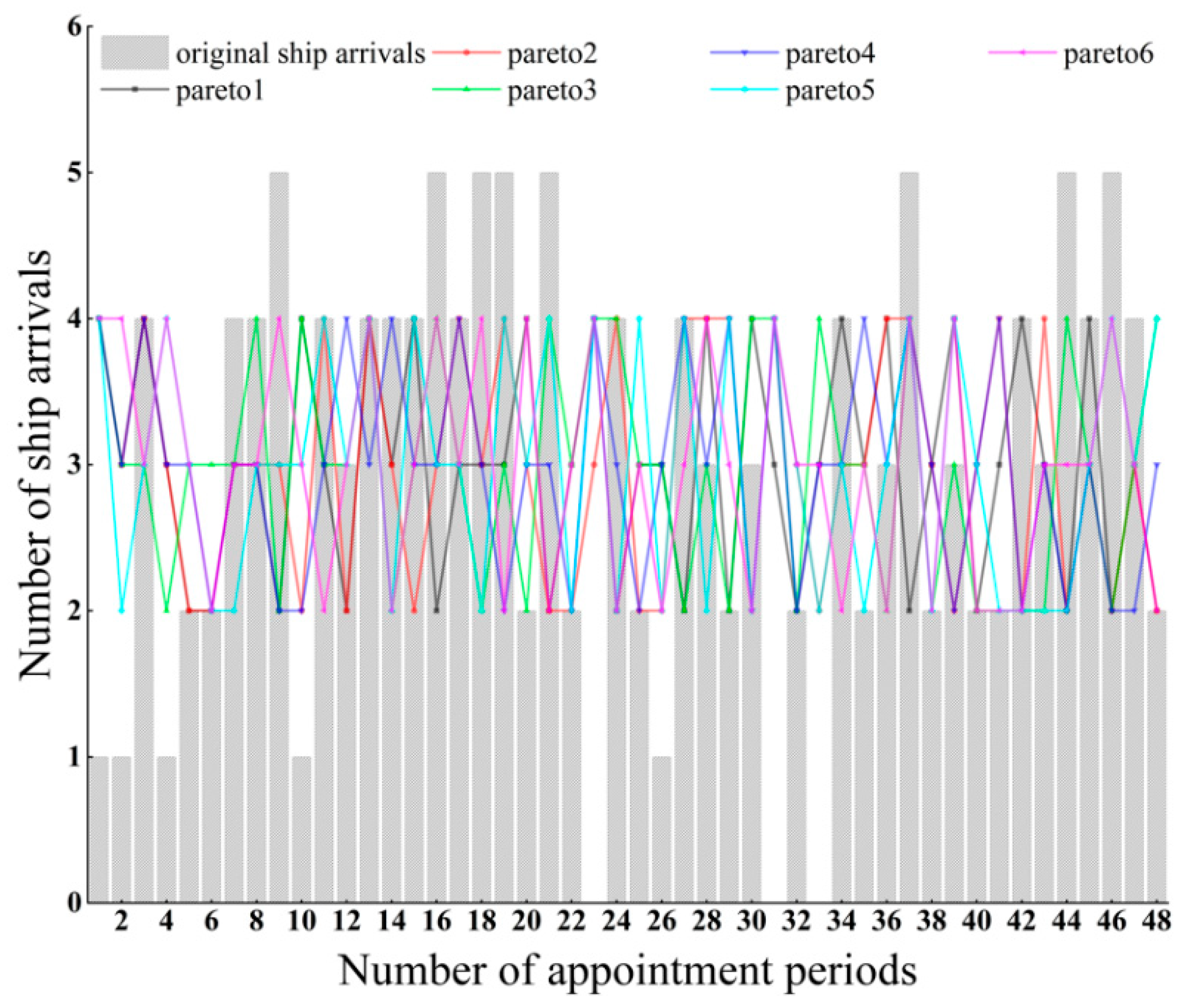
Figure 9 presents the corresponding distribution of scheduled arrival times. While vessel clustering persists in certain intervals with high peaks and fluctuations, the optimized distribution achieves peak-shaving during busy periods and load-filling in low-demand periods, resulting in a more balanced temporal structure. These results suggest that, even without local search mechanisms, the NSGA-II algorithm provides a degree of temporal regulation that helps mitigate congestion caused by concentrated arrivals.

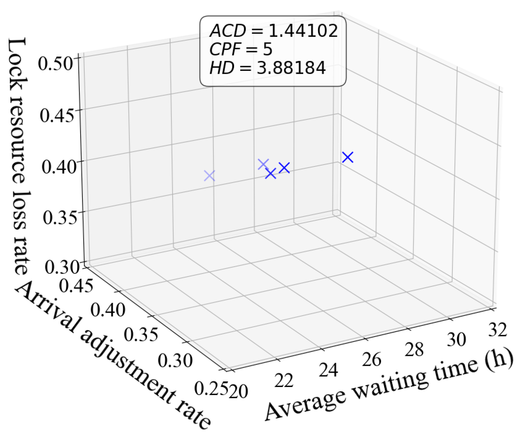
Figure 10 shows the Pareto distribution of optimal appointment scheduling solutions obtained by the VNS-NSGA-II algorithm under uncertain vessel arrival times. The values of ACD, CPF, and HD are 1.44102, 5, and 3.88184, respectively. Compared with NSGA-II, the solution set is denser and exhibits broader boundary coverage, indicating enhanced local search capability through the Variable Neighborhood Search (VNS) mechanism.

Figure 11 presents the corresponding optimized arrival distribution, where fluctuations are reduced, peak congestion alleviated, and low-demand periods partially filled, yielding a smoother and more balanced temporal pattern. Overall, VNS-NSGA-II outperforms NSGA-II in peak-shaving and valley-filling, improving scheduling balance and resource utilization under uncertainty.

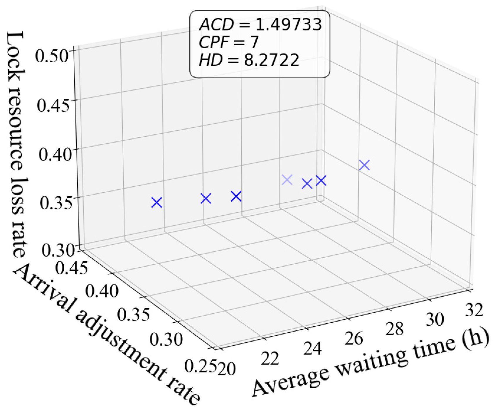
Figure 12 presents the Pareto-optimal solutions obtained by the DE-VNS-NSGA-II algorithm under uncertain vessel arrival times. The values of ACD, CPF, and HD are 1.49733, 7, and 8.2722, respectively, outperforming the other two algorithms. Driven by these maximum indicator values, the resulting Pareto front not only maintains a well-distributed structure but also achieves broader boundary expansion.

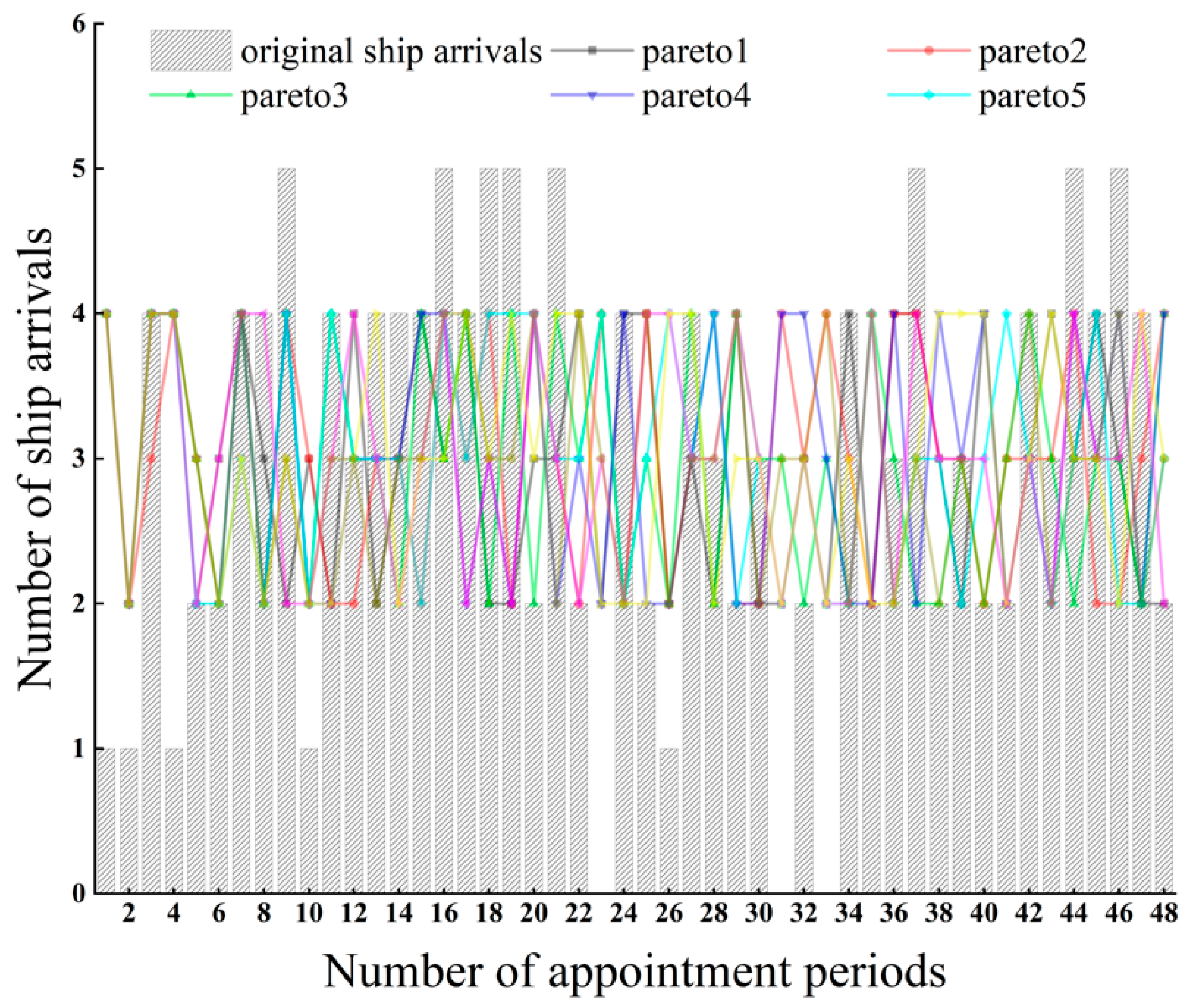
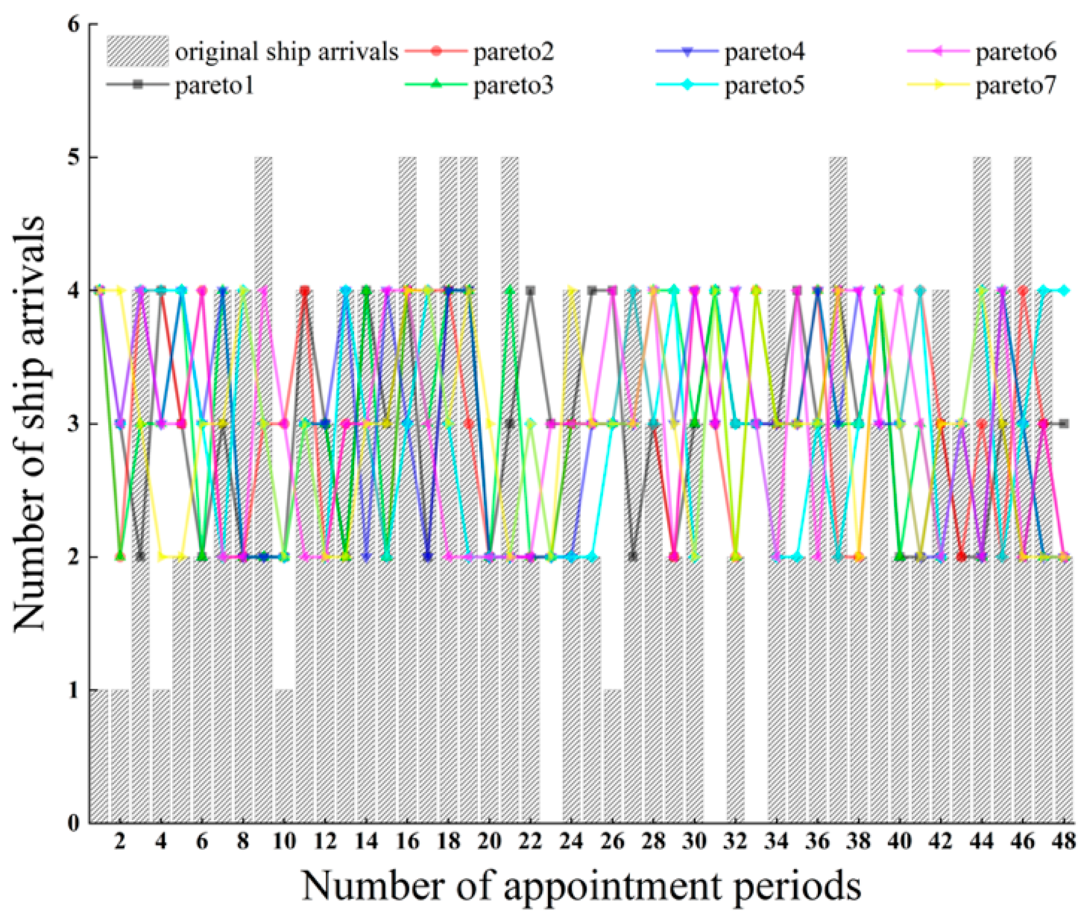
Figure 13 shows the algorithm’s responsiveness to appointment violations, where delayed vessels were dynamically adjusted and reassigned through the re-appointment mechanism. Overall, vessel arrivals across time intervals remained stable, without notable congestion or idle gaps, and the schedule exhibited a high degree of balance. These results confirm that the DE-VNS-NSGA-II algorithm offers enhanced adaptive control and scheduling stability under both arrival uncertainty and operational disturbances, providing robust support for intelligent scheduling in complex navigation environments.

Therefore, it can be concluded that the proposed approach possesses superior global search capabilities and greater robustness than its predecessors.

4.5. Comparative Evaluation of Metaheuristic Algorithms for Vessel Lockage Scheduling Under Uncertainty

To comprehensively evaluate the performance of the proposed DE-VNS-NSGA-II, this section compares it against four well-established and state-of-the-art benchmark evolutionary algorithms. Brief descriptions of these baseline algorithms are provided as follows:

NSGA-II: A popular multi-objective genetic algorithm utilizing fast non-dominated sorting and crowding distance mechanisms to ensure solution diversity and elitism.

VNS-NSGA-II: A hybrid approach embedding Variable Neighborhood Search into NSGA-II to significantly enhance local exploitation capabilities and overall solution quality.

GSAA-RL [42]: A hybrid optimization method merging genetic and simulated annealing algorithms, using reinforcement learning for dynamic parameter adaptation and enhanced search.

ADEA-KC [43]: An adaptive differential evolution algorithm leveraging K-means clustering to guide population mutation strategies, balancing global exploration and local exploitation.

Based on three evaluation metrics: average vessel waiting time (Z₁), appointment adjustment ratio (Z₂), and lock resource loss rate (Z₃) (see

Table 8. Comparison of five algorithms on objective values and computation time.

Algorithms	Objective						CT (s)
	Z1		Z2		Z3
	Value	IR	Value	IR	Value	IR
NSGA-II	28.62531	/	0.33127	/	0.41253	/	215.59
VNS-NSGA-II	24.31683	15.05%	0.30861	6.84%	0.39721	3.71%	363.3
DE-VNS-NSGA-II	23.32713	18.51%	0.30138	9.02%	0.39167	5.06%	342.48
GSAA-RL [42]	23.83417	16.74%	0.30453	8.07%	0.39415	4.46%	1544.82
ADEA-KC [43]	24.95769	12.81%	0.31149	5.97%	0.40135	2.71%	116.72

). The results indicate that DE-VNS-NSGA-II outperforms the other algorithms across all metrics, achieving an average waiting time of 23.32713 h, an adjustment ratio of 0.30138, and a lock resource loss rate of 0.39167.

Table 8 reports the improvement rates (IR) of VNS-NSGA-II and DE-VNS-NSGA-II relative to the baseline NSGA-II across the three objectives, where IR denotes the improvement rate and CT represents the computation time. The results show that DE-VNS-NSGA-II achieves the greatest improvements in all objectives: average waiting time is reduced by 18.51% (from 28.62531 h to 23.32713 h), arrival adjustment ratio by 9.02% (from 0.33127 to 0.30138), and lock resource loss rate by 5.06% (from 0.41253 to 0.39167). By contrast, the improvement rates for VNS-NSGA-II are 15.05%, 6.84%, and 3.71% on the three objectives, respectively; for GSAA-RL, they are 16.74%, 8.07%, and 4.46%; and for ADEA-KC, they are 12.81%, 5.97%, and 2.71%. Notably, DE-VNS-NSGA-II demonstrates more significant improvements in the arrival adjustment ratio and lock resource loss rate, indicating its effectiveness in optimizing population initialization, reducing scheduling adjustments, and enhancing lock resource utilization through variable neighborhood search. We conduct these experiments of comparison performance in the workstation with a CPU of 3.0 GHz and a RAM size of 256 GB. However, due to its more complex process, DE-VNS-NSGA-II required 342.48 s to complete. Despite being more time-consuming than NSGA-II, it outperforms VNS-NSGA-II slightly in terms of speed. Through a performance comparison with new algorithms proposed in recent related papers, we found that although GSAA-RL utilizes reinforcement learning strategies to obtain high-quality solutions, its computation time is as high as 1544.82 s, indicating that it is unsuitable for rapid-response scheduling scenarios. In contrast, ADEA-KC relies on clustering methods to optimize the population structure and achieves an extremely fast solving speed of only 116.72 s; this makes it suitable for scenarios with high real-time requirements, despite its average solution quality.

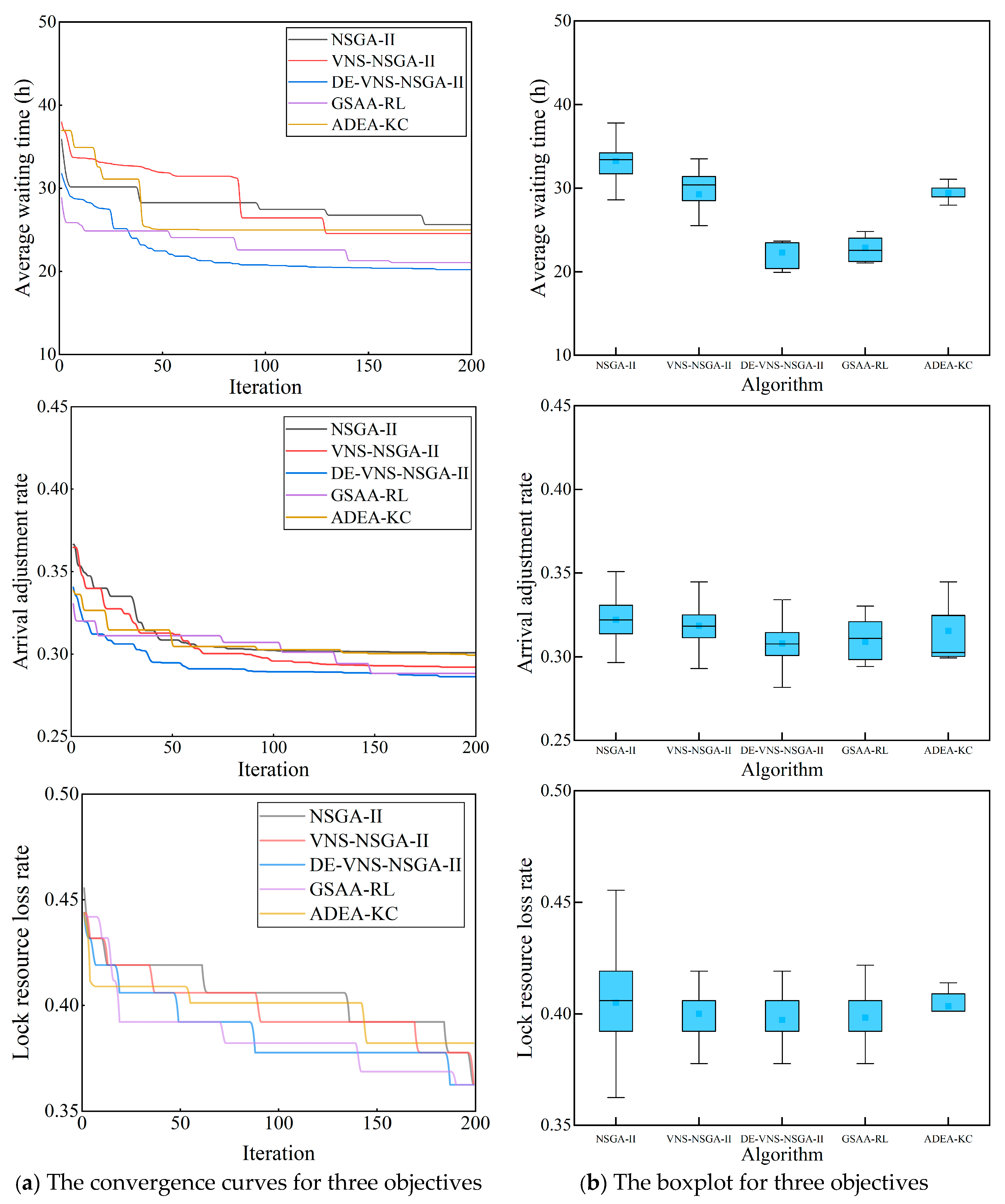
To comprehensively evaluate the overall performance of the proposed algorithm, Figure 14 provides a visual comparison of NSGA-II, VNS-NSGA-II, DE-VNS-NSGA-II, GSAA-RL, and ADEA-KC in terms of convergence speed and solution stability. Figure 14a illustrates the convergence behavior of the algorithms during the iterative process. When simultaneously optimizing the three objectives—average vessel waiting time, appointment adjustment ratio, and lock resource loss rate—DE-VNS-NSGA-II exhibits a highly directed convergence toward stability and resource efficiency. For instance, with respect to average waiting time, DE-VNS-NSGA-II converges to 23.32713 h, whereas the baseline NSGA-II converges to 28.62531 h, and the recently proposed algorithms GSAA-RL and ADEA-KC converge to 23.83417 h and 24.95769 h, respectively. This result indicates that the incorporation of Differential Evolution (DE) and Variable Neighborhood Search (VNS) effectively enhances optimization efficiency compared to both traditional and recent advanced methods.

Beyond convergence speed, solution stability is also essential. As shown in the boxplot comparison in Figure 14b, DE-VNS-NSGA-II consistently achieves lower medians and narrower interquartile ranges across all three objectives. Its boxplots lie substantially below those of the other algorithms, indicating a more compact solution set and reduced variability. These results suggest that the proposed algorithm not only delivers higher-quality solutions but also demonstrates stronger robustness.

In summary, by incorporating Differential Evolution (DE) and Variable Neighborhood Search (VNS) into NSGA-II to enhance local exploration, DE-VNS-NSGA-II achieves concurrent improvements in computational efficiency and solution quality. The algorithm is capable of rapidly generating high-quality scheduling solutions while maintaining stability and reliability, thus outperforming the benchmark algorithms in overall performance.

5. Discussion

5.1. Methodological Advantages

This study proposes an integrated vessel appointment scheduling framework that combines uncertainty quantification, multi-objective optimization, and efficient solution methods. Its contributions and advantages lie in three aspects: the accuracy of the uncertainty quantification model, the superiority of the optimization algorithm, and the robustness of the scheduling scheme.

First, to address the unpredictability of vessel arrival times, a deep ensemble learning-based prediction model was developed for uncertainty quantification. As shown in Table 2, the proposed model (M3) outperforms other models in point prediction, achieving the lowest MAE, RMSE, and MAPE values, thereby confirming its accuracy in capturing the underlying trend. This proposed DE-VNS-NSGA-II model attains a Prediction Interval Coverage Probability (PICP) of 93.45%, exceeding the 90% confidence target, with the narrowest Mean Prediction Interval Width (MPIW) of 22.57 among all benchmarks. This indicates that the model not only provides reliable coverage of actual arrival times but also yields compact and practically useful prediction intervals. By transforming vague uncertainties into mathematically analyzable intervals, this approach establishes a solid data-driven foundation for robust scheduling optimization, consistent with recent developments in transportation prediction research [46].

Second, the proposed DE-VNS-NSGA-II algorithm demonstrates significant advantages in solving complex, large-scale lock scheduling problems. By synergistically integrating the robust global exploration of Differential Evolution (DE) with the deep local intensification of Variable Neighborhood Search (VNS), the algorithm effectively overcomes the premature convergence frequently observed in standard NSGA-II. As demonstrated in Table 4, this hybrid approach yields substantial operational benefits: it reduces the average vessel waiting time by 18.51%, lowers the appointment adjustment ratio by 9.02%, and decreases the lock resource loss rate by 5.06% compared to the baseline NSGA-II. From a practical application perspective, these algorithmic improvements translate into highly stable and predictable lockage schedules. The rapid convergence and robust optimization performance ensure that lock operators can swiftly generate reliable, high-quality rescheduling plans—even under uncertain arrival conditions. Consequently, this algorithmic framework provides a highly efficient, data-driven decision-support tool for real-time inland waterway management [47].

Third, the proposed method demonstrates robust scheduling performance under arrival time uncertainty. Here, robustness is not limited to a single dimension but reflects the ability of the scheduling scheme to sustain system efficiency and resource utilization with minimal adjustment costs. Specifically, by lowering the appointment adjustment ratio to its minimum while simultaneously reducing average waiting time and lock resource loss, the method achieves a balanced trade-off among efficiency, stability, and resource utilization. This approach is consistent with the principles of robust berth allocation [48] and dynamic vehicle routing [49], while extending these concepts to the context of inland lock scheduling. The results highlight the practical applicability of the proposed approach for intelligent scheduling in complex and uncertain operational environments.

5.2. Limitations for Future Improvement

For computational tractability, we model arrival-time prediction errors as Gaussian, which yields closed-form uncertainty intervals and efficient estimation. In practice, however, empirical error distributions often deviate from normality, showing skewness, multimodality, or heteroscedasticity [50], so the Gaussian specification can be imprecise and may degrade coverage calibration and validity under distributional shifts. To mitigate this misspecification, we will relax the Gaussian assumption using distribution-free conformal calibration and more flexible likelihoods or mixtures. In parallel, we will develop a fusion-based deep learning framework that integrates heterogeneous signals via attention-based feature fusion [51]. Models will be trained with robustness-oriented losses and calibrated post hoc with conformal methods to provide better specified and better calibrated uncertainty across routine and perturbed conditions.

This study models rescheduling as a constraint-feasible time slot reallocation that optimizes a predefined set of objectives. While this abstraction improves tractability, it omits important operational principles, including fairness across vessels, implementability within command and acknowledgment workflows, and stability under repeated adjustments. Consequently, solutions may perform well on the specified objectives yet be difficult to implement or accept in practice. To better align with real operations, the formulation will explicitly encode fairness within the multi-objective model using measures such as equity of waiting and minimax delay criteria, consistent with observations in berth-allocation research where fairness is often secondary to efficiency [52]. Implementability will be strengthened by making the command–acknowledgment–execution pipeline explicit, with lead times, acceptance decisions, and resource availability modeled as decision-linked constraints [53]. Within the feasible region defined by these operational constraints, Pareto-efficient plans will be generated using multi-objective methods already common in maritime scheduling, and candidate schedules will then be validated with agent-based or rolling-horizon tests to reflect dynamic arrivals and operational feedback in ports and locks [18,54].

6. Conclusions

This study advances a robustness-oriented lock-reservation scheduling framework that explicitly accounts for uncertainty in vessel arrivals. Arrival-time uncertainty is quantified with a deep ensemble incorporating real-time hydrological and traffic features, furnishing calibrated probabilistic inputs. A multi-objective formulation, supported by a bidirectional rescheduling mechanism, then reconciles efficiency, schedule stability, and lock-chamber utilization. Notably, maximizing lock utilization inherently generates a flow-smoothing effect that attenuates uncertainty propagation for downstream facilities. The resulting problem is solved efficiently with the hybrid heuristic DE–VNS–NSGA-II to yield implementable schedules. Using real operational data, our simulation experiments show substantial gains over the benchmark: average vessel waiting time decreases by 18.51%, the schedule-adjustment rate by 9.02%, and lock-chamber resource loss by 5.06%. Taken together, these improvements indicate that the proposed approach enhances adaptability and overall scheduling performance under arrival-time uncertainty, providing a robust, practice-oriented basis for intelligent traffic management in complex inland waterway environments. From a practical application perspective, lock operators can utilize the predicted uncertainty intervals to dynamically adjust appointment quotas and issue early warnings to vessels. Furthermore, the automated rescheduling mechanism provides a systematic protocol to dynamically reassign time slots, directly reducing the reliance on inefficient manual interventions during operational disruptions.

Despite these gains, the current study has certain limitations that outline future research directions. First, we model arrival errors as Gaussian and do not explicitly encode implementability or fairness in rescheduling. Next, we will relax the Gaussian assumption via conformal calibration and flexible likelihoods, and embed fairness and workflow-compatible constraints to obtain well-calibrated and executable schedules.