Structural Deformation Prediction and Uncertainty Quantification via Physics-Informed Data-Driven Learning

Abstract

In structural health monitoring, purely data-driven methods for deformation prediction are often susceptible to time-varying boundary conditions under complex operating scenarios, leading to insufficient physical interpretability and limited generalization across different conditions. To address these challenges, this study proposes a Physics-Informed Dual-branch Long Short-Term Memory framework (PINN-DualSHM). The framework employs dual-branch LSTMs to separately extract temporal features of structural mechanical responses and environmental thermal effects. Dynamic decoupling and fusion of these heterogeneous features are achieved through an adaptive cross-attention mechanism. Furthermore, physical priors, including the thermodynamic superposition principle and structural settlement monotonicity, are embedded into the loss function as regularization terms, complemented by a dual uncertainty quantification system based on heteroscedastic regression and MC Dropout. Experimental results based on long-term measured data from an industrial base project in Shenzhen demonstrate that PINN-DualSHM significantly outperforms baseline models such as LSTM, CNN-LSTM, and GAT-LSTM. Specifically, the Root Mean Square Error (RMSE) is reduced by 65.25%, and the coefficient of determination (R²) reaches 0.925. Physical consistency analysis confirms that the introduction of physical constraints effectively suppresses anomalous predictive fluctuations that violate mechanical laws. Uncertainty decomposition reveals that aleatoric uncertainty is dominant (93.7%), objectively indicating that the current system’s accuracy bottleneck lies in sensor noise rather than model capability. By enhancing prediction accuracy while providing credible quantitative assessments and physical interpretability, the proposed method provides a scientific basis for the operation, maintenance optimization, and upgrading decisions of SHM systems.

1. Introduction

Structural safety is related to public security and social stability. Statistical data shows that the existing urban building area in China is approximately 24.8 billion square meters, which includes 1.04 million dilapidated buildings and numerous historical structures. Given the large building inventory and ongoing structural aging, real-time deformation prediction based on monitoring data is important for risk warning and failure prevention. Traditional numerical or physical prediction methods, such as consolidation theory and finite element analysis, rely on accurate stratigraphic parameters and boundary conditions. However, these parameters are difficult to obtain accurately in practice. The model calibration process is complex, and it is difficult to fully account for factors like soil anisotropy, nonlinear seepage, and construction disturbances. Furthermore, these methods have limited online data assimilation capabilities and cannot dynamically update predictions as monitoring data accumulates, restricting their applicability in long-term maintenance.

To address the limitations of traditional methods in data assimilation, deep learning methods have been applied to structural deformation prediction. Convolutional Neural Networks (CNNs) [1,2,3,4,5,6,7,8], Generative Adversarial Networks (GANs) [9,10,11], and Long Short-Term Memory (LSTM) networks [12] have shown nonlinear fitting capabilities in multi-factor coupled time-series forecasting. Nevertheless, purely data-driven models have inherent limitations [13]. First, the physical interpretability of the models is low; they cannot distinguish between mechanical and thermal strains, and the prediction results can violate basic physical laws. Second, they depend on large sample sizes, making them prone to overfitting in scenarios with sparse data. Third, they lack uncertainty quantification mechanisms and cannot provide confidence intervals. Finally, their generalization ability is limited, and prediction accuracy decreases under varying boundary conditions or unseen operational states.

To address the generalization and interpretability issues of purely data-driven methods, hybrid modeling approaches represented by Physics-Enhanced Machine Learning (PEML) have been studied in structural health monitoring. Physics-Informed Neural Networks (PINNs) [14] introduce governing equations or physical priors into the loss function, providing a physically constrained approach for data-driven modeling. Haywood-Alexander et al. [15] reviewed three implementation routes for PEML in monitoring and digital twins. Liu et al. [16] applied a physics-guided deep Markov model to identify uncertain nonlinear dynamical systems. Lai et al. [17] applied physics-informed neural ordinary differential equations to structural parameter identification. Additionally, Cianci et al. [18,19] constructed a PEML-based grey-box predictive model and an Early Warning System (EWS), achieving environmental effect filtering and decoupling in bridge bearing displacements. These studies confirm the effectiveness of physical constraints in improving model generalization, robustness, and interpretability.

However, the application of PINNs and uncertainty quantification (UQ) in engineering still faces objective limitations. Regarding physical constraints, standard PINNs rely on minimizing the residuals of partial differential equations (PDEs). Due to unclear boundary conditions and sparse sensor deployments in actual buildings, it is difficult to calculate high-order spatiotemporal derivatives accurately. Meanwhile, existing studies mostly focus on a single physical field, with less research on the joint modeling of multi-source heterogeneous monitoring signals. Many methods use fixed physical constraint weights and do not adaptively adjust them based on dynamic features during training. Regarding UQ, current studies rarely decompose epistemic and aleatoric uncertainties simultaneously. Bayesian Neural Networks (BNNs) provide posterior distributions but involve high computational costs, making it difficult to apply to long-sequence multi-step forecasting. Deep Ensembles incur high deployment costs. The MC Dropout method is relatively lightweight, but its estimation is sensitive to hyperparameters, and it lacks calibration guidelines for civil engineering monitoring scenarios [20].

To address these limitations, this study proposes a physics-informed dual-branch long short-term memory network framework (PINN-DualSHM). This framework models structural strain and environmental temperature signals separately through a dual-branch LSTM encoder, and it uses an adaptive cross-attention mechanism for the dynamic weighted fusion of multi-source heterogeneous features. To avoid the computational difficulties of solving complex PDEs, this study formulates the thermodynamic superposition principle and structural monotonicity as soft constraints embedded in the joint loss function, maintaining the physical rationality of the predictions. Simultaneously, a decomposition framework combining heteroscedastic regression and MC Dropout is used to quantify epistemic and aleatoric uncertainties. This study aims to supplement existing methods in physical consistency, multi-source fusion, and UQ, providing a quantitative basis for the maintenance optimization and risk decision-making of monitoring systems.

2. Fundamental Principles

2.1. Deformation Mechanism and Construction of Physics Constraints

In structural engineering, the displacement at an arbitrary point is jointly governed by the internal stress and strain states, which can be described by the kinematic equations, constitutive relations, and thermodynamic relationships. According to the thermodynamic superposition principle, the total strain can be decomposed into mechanical strain induced by external loads and thermal strain induced by temperature variations. The thermal strain follows the linear law of thermal expansion with respect to temperature change. By combining the above relations, a partial differential equation governing settlement displacement can be derived, in which the external term is determined by the loading conditions and boundary constraints.

$$\epsilon (z)={\displaystyle \frac{du(z)}{dz}}$$

(1)

Equation (1) defines the kinematic relationship between strain and displacement under the assumption of one-dimensional (1D) small deformation, where $u(z)$ represents the axial displacement at depth $z$, and $\epsilon (z)$ denotes the normal strain. The rationale for this 1D simplification is twofold: first, the settlement deformation in this project is predominantly characterized by vertical compression with sufficient lateral constraints, allowing lateral displacement components to be neglected; second, the longitudinal geometric dimension of the monitored section is significantly larger than its transverse dimensions, satisfying the plane-section (Euler-Bernoulli) assumption, which renders linearized strain valid within the margin of engineering precision.

$$\sigma =E\cdot {\epsilon }_{\mathrm{mech}}$$

(2)

Equation (2) presents the linear elastic constitutive equation (Hooke’s Law), where $E$ is the equivalent elastic modulus of the soil or structure. It is assumed that only the mechanical strain ${\epsilon }_{\mathrm{mech}}$ contributes to stress, whereas the free thermal expansion induced by temperature does not directly generate stress (in the absence of constraints). The linear elastic assumption aligns well with field-measured data within the normal service load range, while any nonlinear effects exceeding the elastic limit are implicitly captured by the data-driven component of the proposed model.

$${\epsilon }_{\mathrm{total}}={\epsilon }_{\mathrm{mech}}+\alpha \Delta T$$

(3)

Equation (3) decomposes the total strain into two components: mechanical strain and thermal strain, where $\alpha$ is the coefficient of thermal expansion and $\Delta T$ is the temperature difference relative to the reference temperature. This decomposition serves as the essential prerequisite for the validity of Equation (4) and provides the theoretical foundation for incorporating temperature sensor data into the physical constraints of the network.

$${\displaystyle \frac{d}{dz}}\left\{E\cdot \left({\displaystyle \frac{du(z)}{dz}}-\alpha \Delta T(z)\right)\right\}+f(z)=0$$

(4)

As previously discussed, standard Physics-Informed Neural Networks (PINNs) provide a foundational framework for physics-constrained modeling. However, practical engineering applications often suffer from sparse sensor distribution, material degradation, and time-varying boundary conditions. Under these limitations, directly solving partial differential equations (PDEs) as hard constraints frequently leads to difficulties in computing high-order derivatives and causes training instability.

Considering these objective limitations, this study does not directly solve the governing PDEs for structural deformation. Instead, inspired by the core concept of PINNs, the key physical mechanisms are formulated as soft constraints and embedded into the loss function. Specifically, the aforementioned equations and mechanical relationships are incorporated into the training process as implicit penalty terms. If the model predictions violate fundamental physical laws, such as mechanical equilibrium, the loss function automatically imposes a penalty. Compared to explicitly solving PDEs, this approach provides greater engineering flexibility. It can better accommodate the time-varying nature of external loads and the spatial heterogeneity of foundation parameters [14]. Centered on the intrinsic physical relationships of structural deformation, this study constructs the following three core physical constraints, which effectively introduce prior mechanistic information while ensuring stable model training:

(1) Strain Consistency Constraint ($L_{sn}$): Based on the thermodynamic superposition principle, this constraint enforces that the sum of the predicted mechanical strain and thermal strain should be consistent with the total strain measured by sensors, expressed as:

$${\epsilon }_{total}={\epsilon }_{mech}+{\epsilon }_{th}$$

(5)

where ${\epsilon }_{total}$ denotes the total strain measured by sensors, and ${\epsilon }_{mech}$ and ${\epsilon }_{th}$ represent the model-predicted mechanical strain and thermal strain, respectively.

(2) Temperature-Thermal Strain Relationship Constraint ($L_{th}$): Based on the thermal expansion characteristics of materials, this constraint enforces that thermal strain is proportional to temperature variation, expressed as:

$${\epsilon }_{th}\approx \alpha \cdot \Delta T$$

(6)

where $\alpha$ denotes the coefficient of thermal expansion. Considering that this parameter may vary with material aging in practical engineering applications, it is configured as a learnable parameter in this study, enabling the model to adaptively identify it from data.

(3) Strain-Settlement Monotonic Constant ($L_{mc}$): According to the principle of mechanical structure, when the strain increases, the settlement shows a monotonic state. This constant penalty violates the physical monotonic prediction, making the model output more physically reasonable.

The aforementioned multi-level physical constraint design avoids the computational difficulties associated with calculating derivatives for complex PDEs. If the model predictions violate fundamental principles such as boundary force equilibrium or monotonicity, the loss function automatically imposes an implicit penalty. Compared to explicitly solving PDEs, this approach offers greater flexibility. It can effectively accommodate time-varying loads and the spatial heterogeneity of foundation parameters. Furthermore, while ensuring engineering deployability, it significantly enhances the physical consistency and training stability of the model under complex, unseen conditions.

2.2. Long Short-Term Memory (LSTM)

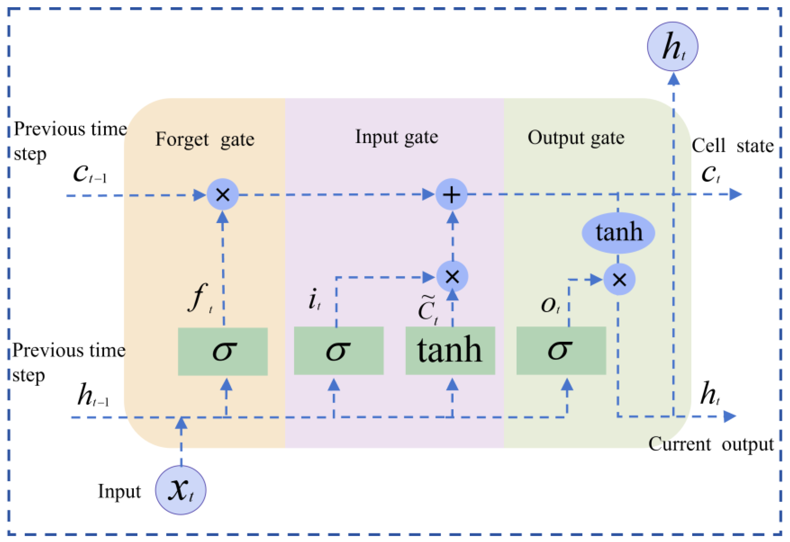
Recurrent Neural Networks (RNNs) use a recursive structure to model sequence dependencies and are applied in time series tasks. However, conv RNNs encounter the problems of gradient vanishing and explosion when dealing with long-sequence learning. This not only hinders the retention of long-term information but also makes the stability and convergence of training worse. Hochreiter et al. proposed LSTM nets [21,22]. LSTM uses a gating mechanism to regulate the forgetting, writing, and output of information, and introduces a cell state as an information channel across time steps. Design the ability to enhance long-term dependence, and also relieve the problem of gradient disappearance to a certain extent. Figure 1 shows the basic architecture of the LSTM unit.

Engineering applications show that LSTM is more robust and generative than traditional RNN [23,24]. Its gating mechanism can suppress noise and filter out irrelevant fluctuations, and enhance the selection and extraction of key time features. Therefore, LSTM is a commonly used deep learning model in tasks such as dynamic system response prediction, nonlinear time series modeling, and engineering structure health monitoring.

Structural health monitoring sequence data typically exhibit nonlinearity and distributed lag effects. In this study, a unidirectional long short-term memory (LSTM) network is utilized as the core of the encoder. By integrating historical context information within the observation window, the LSTM network effectively captures temporal dependencies. This approach facilitates a clear description of the influence of the thermal lag effect and strain accumulation effect on the structural response.

2.3. Uncertainty Quantification Mechanism

In structural health monitoring (SHM) applications, single point predictions cannot reflect the reliability boundaries of the results, limiting the objectivity of risk assessment and maintenance decision-making. Therefore, introducing probabilistic forecasting and quantifying uncertainty is necessary [25]. Within a statistical framework, uncertainty is primarily categorized into aleatoric uncertainty and epistemic uncertainty. Aleatoric uncertainty originates from the inherent randomness of the system. It is an irreducible component, typically characterized by learning the distribution parameters of the predicted data. Conversely, epistemic uncertainty reflects a lack of model knowledge. It is usually caused by model structural limitations, parameter estimation biases, and incomplete training data coverage. Theoretically, this uncertainty can be reduced by supplementing data or improving the model.

To achieve joint assessment of both types of uncertainty, this study adopts a hybrid mechanism combining heteroscedastic regression with MC Dropout. Epistemic uncertainty is estimated through Monte Carlo Dropout (MC Dropout), which can be viewed as an approximate inference of Bayesian Neural Networks (BNN). Bayesian neural networks assign a prior distribution $W$ to the weights $p(W)$ and infer the posterior distribution $p(W\left|X,Y)\right.$ conditioned on observed data $X,Y$. Since the posterior distribution is typically intractable analytically, MC Dropout maintains active Dropout layers during both training and inference phases to achieve variational approximation of the weight posterior. During inference, performing $T$ stochastic forward passes yields a predictive distribution ${\left\{{\widehat{y}}_t\right\}}_{t=1}^T$ composed of $T$ prediction samples.

Aleatoric uncertainty is characterized through heteroscedastic regression. This study augments the prediction head with a variance output branch, enabling the model to output both the predicted mean of settlement ($\mu$) and the variance ${\sigma }_{ac}^2$ simultaneously. The model is trained end-to-end by maximizing the Gaussian likelihood, with the loss function formulated as follows:

$$L_{nll}={\displaystyle \frac{1}{2{\sigma }_{ac}^2}}{||y-\mu ||}^2+{\displaystyle \frac{1}{2}}\log ({\sigma }_{ac}^2)$$

(7)

This loss function encourages the model to output larger variance when noise is strong or patterns are unclear, while outputting smaller variance when patterns are stable.

The final uncertainty statistics are defined as follows. The predicted mean is given by:

$$\widehat{\mu }={\displaystyle \frac{1}{T}}{\displaystyle \sum {\mu }_i}$$

(8)

Epistemic uncertainty is computed as:

$${\sigma }_{ec}^2={\displaystyle \frac{1}{T}}{\displaystyle \sum {({\mu }_i-\widehat{\mu })}^2}$$

(9)

Aleatoric uncertainty is expressed as:

$${\sigma }_{ac}^2={\displaystyle \frac{1}{T}}{\displaystyle \sum {\sigma }_{ac,i}^2}$$

(10)

Total uncertainty is obtained by:

$${\sigma }_{total}^2={\sigma }_{ec}^2+{\sigma }_{ac}^2$$

(11)

In terms of implementation, the model keeps Dropout active during inference only in the fusion projection layer and the mean prediction head to estimate epistemic uncertainty. Conversely, Dropout within the LSTM encoder serves merely as a regularization technique during training and is deactivated during inference. The final model output consists of the predicted mean and the total variance. The former provides a point estimate, while the latter indicates the overall predictive uncertainty level.

The uncertainty decomposition results provide an objective basis for subsequent engineering maintenance decisions. When epistemic uncertainty dominates, it indicates that current operational conditions may fall outside the coverage of the training data. In this case, supplementing measured data or recalibrating the model is recommended. When aleatoric uncertainty dominates, according to Kendall and Gal [20], this uncertainty originates not only from sensor measurement noise. It also encompasses unmodeled dynamic effects (such as local foundation heterogeneity and construction load fluctuations), missing covariates (such as groundwater levels and seasonal temperature accumulation), and approximation errors of physical constraints, alongside other inherent random factors.

According to general findings in deep learning uncertainty quantification, when a model is sufficiently trained on an adequate dataset, epistemic uncertainty is typically much lower than aleatoric uncertainty [26]. If the model’s decomposition results exhibit this pattern, it indicates that the model parameters have largely converged on the existing data and possess good stability. In such scenarios, the system’s uncertainty is primarily driven by external noise and measurement errors. Therefore, from an engineering perspective, priority should be given to improving sensing system hardware and data collection quality.

3. Construction of Physics-Informed Dual-Branch LSTM Prediction Model

3.1. Physics-Constrained Joint Loss Function

To balance the numerical accuracy and physical consistency of the settlement prediction, this study formulates the model training as a multi-objective optimization problem. The joint loss function consists of a weighted combination of a data-driven loss and physical regularization terms:

$$L_{total}=L_{data}+{\lambda }_1{L}_{sn}+{\lambda }_2{L}_{th}+{\lambda }_3{L}_{mc}+{\lambda }_4{L}_{nll}$$

(12)

where $L_{data}$ represents the data-driven loss, and ${\lambda }_i$ are the weight coefficients for the physical regularization and uncertainty terms, adjusting their contributions to the total loss. These weights remain fixed during training, and their specific values are determined based on dimensional balance and gradient magnitude matching observed in preliminary experiments.

The data-driven loss employs a weighted combination of Mean Squared Error (MSE) and Pearson correlation loss:

$$L_{data}=w_{mse}\cdot L_{MSE}+w_{corr}\cdot L_{corr}$$

(13)

The MSE is calculated point-by-point across the sample and time-step dimensions to constrain the absolute accuracy of the predicted values:

$$L_{MSE}={\displaystyle \frac{1}{B\cdot T_p}}{\displaystyle \sum _{b=1}^B{\displaystyle \sum _{k=1}^{T_p}{({\widehat{y}}_{b,k}-y_{b,k})}^2}}$$

(14)

where B is the batch size, $T_p$ is the number of prediction steps, and ${\widehat{y}}_{b,k}$ and $y_{b,k}$ are the predicted and measured settlements of the b-th sample at the k-th step, respectively.

The correlation loss is based on the Pearson correlation coefficient. It is calculated by flattening the predicted and measured values within a batch to constrain the overall temporal trend:

$$L_{corr}=1-{\displaystyle \frac{{\displaystyle \sum _i({\widehat{y}}_i-\overline{\widehat{y}})}(y_i-\overline{y})}{\sqrt{{\displaystyle \sum _i{({\widehat{y}}_i-\overline{\widehat{y}})}^2}+ϵ}\cdot \sqrt{{\displaystyle \sum _i{(y_i-\overline{y})}^2}+ϵ}}}$$

(15)

where $ϵ={10}^{-8}$ is a numerical stability term to prevent division by zero. The MSE focuses on correcting amplitude deviations, while the correlation loss focuses on maintaining trend consistency. The two complement each other to jointly improve the numerical fitting and temporal morphological prediction.

The physical constraints and uncertainty terms consist of the three previously extracted physical constraints and a negative log-likelihood term for aleatoric uncertainty, detailed as follows:

(1)

Strain Consistency Constraint

Based on the thermodynamic strain superposition principle, the sum of the mechanical strain and thermal strain predicted by the model is required to approximate the measured total strain within the complete observation window. The residual of this constraint is aggregated in a mean square format across the time and sensor node dimensions:

$$L_{sn}={\displaystyle \frac{1}{T_{obs}\cdot N_s}}{\displaystyle \sum _{t=1}^{T_{obs}}{\displaystyle \sum _{n=1}^{N_s}{({\epsilon }_{total}^{t,n}-{\widehat{\epsilon }}_{mech}^{t,n}-{\widehat{\epsilon }}_{th}^{t,n})}^2}}$$

(16)

where $N_s$ is the number of structural strain sensor nodes. This term ensures that physical consistency holds throughout the entire historical observation sequence.

(2)

Temperature and Thermal Strain Relationship Constraint

Based on the material’s thermal expansion characteristics, this term constrains the predicted thermal strain to be proportional to the temperature increment. The temperature increment is defined as the temperature difference of the current time step relative to the initial step of the observation window. The constraint residual is defined as:

$$L_{th}={\displaystyle \frac{1}{T_{obs}\cdot N_s}}{\displaystyle \sum _{t=1}^{T_{obs}}{\displaystyle \sum _{n=1}^{N_s}{({\widehat{\epsilon }}_{th}^{t,n}-\alpha \cdot \Delta T^t)}^2}}$$

(17)

where the thermal expansion coefficient $\alpha$ is set as a learnable parameter, initialized to ${\alpha }_0=1.2\times {10}^{-5}/°\mathrm{C}$. To accommodate long-term parameter drift caused by factors such as material aging, is adaptively corrected in a data-driven manner.

(3)

Settlement Monotonicity Constraint

The project is located on a coastal soft soil foundation. Under continuous gravity and consolidation effects, the settlement primarily exhibits a long-term unidirectional accumulation pattern. Accordingly, a monotonicity soft constraint is applied to the prediction sequence to penalize abnormal rebound, while allowing reasonable short-term fluctuations caused by groundwater, elastic deformation, etc. In the measured daily-scale data, approximately 49.5% of adjacent steps are non-monotonic, which aligns with engineering phenomena such as tides and elastic deformation. On a monthly scale, about 79% show unidirectional accumulation, consistent with consolidation theory. Therefore, this constraint is positioned as a regularization against long-term trend violations rather than a hard constraint for every step. It adopts a ReLU form: a penalty is generated when ${\widehat{y}}_{k+1}<{\widehat{y}}_k$, and the gradient is zero when ${\widehat{y}}_{k+1}\ge {\widehat{y}}_k$, avoiding interference with physically compliant predictions.

$$L_{mc}={\displaystyle \frac{1}{T_p-1}}{\displaystyle \sum _{k=1}^{T_p-1}\max }(0,-({\widehat{y}}_{k+1}-{\widehat{y}}_k))$$

(18)

(4)

Negative Log-Likelihood Term

To support probabilistic forecasting and heteroscedastic aleatoric uncertainty quantification, the prediction head simultaneously outputs the settlement mean and variance. The model is trained by maximizing the Gaussian likelihood, which is equivalent to minimizing the negative log-likelihood:

$$L_{nll}={\displaystyle \frac{1}{B\cdot T_p}}{\displaystyle \sum _{b=1}^B{\displaystyle \sum _{k=1}^{T_p}\left[\frac{{(y_{b,k}-{\widehat{\mu }}_{b,k})}^2}{2{\widehat{\sigma }}_{b,k}^2+ϵ}+\frac{1}{2}\ln ({\widehat{\sigma }}_{b,k}^2+ϵ)\right]}}$$

(19)

where $ϵ={10}^{-6}$ is a numerical stability term. This term encourages the model to output a larger variance when the pattern is ambiguous or the noise is high, and a smaller variance when the pattern is stable, achieving input-adaptive uncertainty estimation.

The configuration of weight coefficients in the joint loss function follows the principles of dimensional balance and gradient stability. Preliminary experiments observed significant differences in the gradient magnitudes of various unweighted loss terms. To prevent a single loss term from dominating the optimization process, this study uses the weight of the data-driven loss as a baseline to scale the other terms. Specifically, larger weight values are assigned to the strain consistency and temperature-thermal strain constraints to ensure the effective restriction of physical laws. Smaller weight values are assigned to the monotonicity constraint and uncertainty terms, which primarily serve for regularization and calibration.

Table 1. Weight configurations for the joint loss function.

Category	Weight Symbol	Corresponding Loss Term	Value
Data-driven	$w_{mse}$	Mean Squared Error (MSE)	1.0
	$w_{corr}$	Pearson correlation loss	0.2
Physical constraints	${\lambda }_1$	Strain consistency constraint	0.8
	${\lambda }_2$	Temperature-thermal strain relationship constraint	1.0
	${\lambda }_3$	Settlement monotonicity constraint	0.5
Uncertainty	${\lambda }_4$	Negative log-likelihood term	0.15

lists the specific configuration of these weights, achieving a balance between data fitting and physical priors while considering both convergence speed and generalization accuracy.

3.2. Adaptive Cross-Attention Fusion Mechanism

Heterogeneous sensor data fusion, directly splicing or averaging may lead to information dilution and noise amplification, especially when the environmental variables and structures have dynamically changing variables for the settings under different operations. Static fusion cannot capture the correlations accompanying time changes. To solve this problem, this study introduces an adaptive cross-attention mechanism, dynamically allocates fusion weights to different modal features according to the environmental state, so that the fusion representation is more effective and more robust.

The environmental feature encoding vector takes the query and structural information as keys and values. Such a setup enables the model to adaptively select structural information important for settlement under specific environmental states. In addition, a gating module is introduced by introducing the temperature fluctuation intensity. The standard deviation of the temperature sequence measures the environmental disturbance intensity and generates adaptive weights through a learnable gate:

$$\left\{\begin{array}{l}\beta =\sigma (W_{\beta }\cdot [{\sigma }_T,H_{env},H_{st}]+b_{\beta })\\ H_{fu}=\beta \cdot Attention(Q,K,V)+(1-\beta )\cdot H_{st}\end{array}\right.$$

(20)

where $\beta \in [0,1]$ represents the adaptive weight, and $W_{\beta }$ and $b_{\beta }$ are learnable parameters. Large temperature fluctuations lead to weight gain, and the model relies more on fused features to play a role. Small temperature fluctuations lead to weight loss, and at this time the model mostly relies on the characteristics of the structure branch itself. This mechanism enables the model to adjust the fusion strategy by itself for different situations, thereby enhancing the robustness in various environments.

3.3. Overall Architecture of PINN-DualSHM

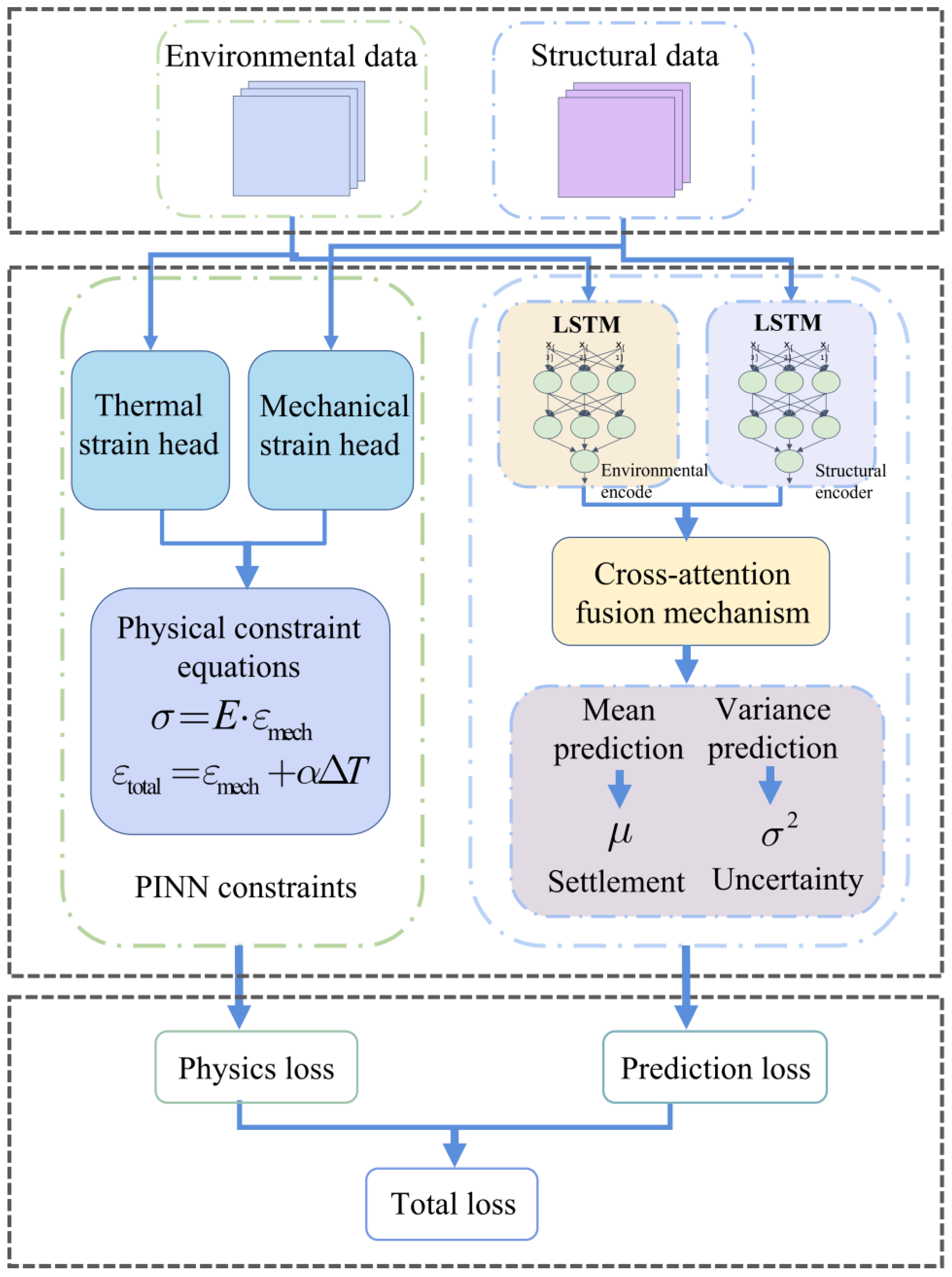
Based on the aforementioned modules, this study constructs the PINN-DualSHM end-to-end prediction framework. The architectural flowchart of the framework is illustrated in Figure 2, which has three stages: feature encoding, dynamic fusion, and probability decoding. Due to the sparse spatial distribution of monitoring nodes and the limitation of engineering computing resources, a lightweight bidirectional LSTM is used to construct parallel dual branches in the encoding stage. The two branches respectively extract features related to structural mechanical response and environmental hysteresis effect. Then, the adaptive cross-attention mechanism is used to dynamically adjust the weights of these heterogeneous features and perform global aggregation. The aggregated features are input into the feedforward prediction head for direct multi-step prediction, reducing the error accumulation risk often associated with autoregressive decoding.

To enhance physical consistency and the credibility of results, the model integrates a physical constraint branch and an uncertainty quantification mechanism. The physical constraint branch decouples force and thermal strain components from the encoded features and uses a physical loss function to regularize the main prediction path. This integration increases the physical consistency of the output. The probability prediction component combines the mean and variance of the prediction head and uses MC Dropout for inference. This method achieves the joint estimation of epistemic and aleatory uncertainties, improves the generalization performance of the model, and enhances its engineering application value.

4. Engineering Case Study and Data Analysis

4.1. Project Overview

This study verifies the engineering applicability of the PINN-DualSHM framework based on measured data from an industrial base project in Shenzhen. The building is a frame-shear wall structure with two underground floors and ten above-ground floors, covering a total construction area of approximately 33,564 m². It is located in a coastal soft soil foundation area. Under the long-term combined effects of seasonal temperature and humidity alternation and surrounding traffic loads, its structural deformation exhibits significant nonlinear and time-varying characteristics, which increases the complexity of deformation prediction.

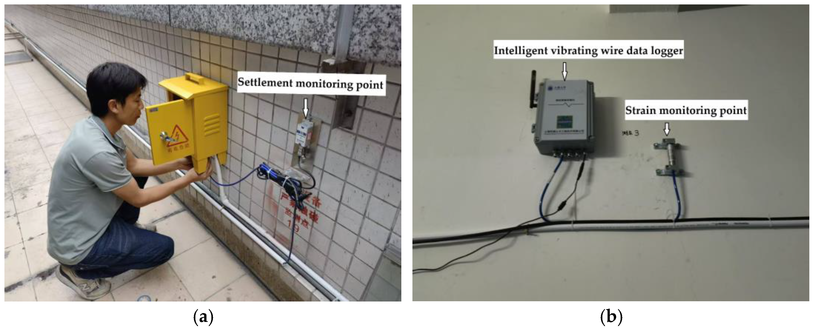
According to the mechanical characteristics of the structure, the on-site monitoring network is deployed at key load-bearing locations (as shown in Figure 3). The system utilizes vibrating wire strain gauges to collect the strain responses of the shear walls and frame columns (key measurement points are YB3 and YB4). It employs hydrostatic levelers to obtain building settlement data as the predictive target of the model, and synchronously records the ambient and structural surface temperatures to objectively quantify the coupling effect of the temperature field on structural deformation.

The experiment extracts continuous monitoring data from 12 October 2023 to 2 July 2025 (with a sampling interval of 8 h). After data cleaning, a total of 1798 valid time steps are obtained. The dataset is sequentially divided into training, validation, and test sets at a ratio of 7:2:1. To eliminate the dimensional differences of the multi-source heterogeneous data, all input variables undergo Z-score standardization before training.

Regarding sample construction, this study adopts a sliding window strategy. The model takes the strain and temperature sequences of 40 historical time steps as joint inputs to fully extract the long-term temporal dependence characteristics of the structural response. It directly outputs the predicted settlement values of the target monitoring point for the next 6 time steps, achieving multi-step forward prediction. During the inference phase, the model combines the MC Dropout technique (configured with 50 forward samples) and the variance prediction branch to synchronously quantify epistemic uncertainty and aleatoric uncertainty. This mechanism decomposes the total predictive uncertainty into two interpretable and independent components, ultimately providing a predictive interval with probabilistic confidence for engineering maintenance and risk decision-making.

4.2. Experimental Setup

The proposed PINN-DualSHM model is implemented using the PyTorch 2.8.0 framework. In the network architecture, the dual-branch encoder employs unidirectional LSTMs with a hidden layer dimension of 64. The feature fusion module utilizes a 4-head adaptive cross-attention mechanism with an output dimension of 128. The prediction module consists of a 256-dimensional mean prediction branch and a 128-dimensional variance prediction branch. Model training uses the Adam optimizer with a batch size of 32 and an initial learning rate of 0.0001. Specific model parameters and training configurations are detailed in

Table 2. Model parameters and training configurations.

Category	Parameter	Value
Data sampling	$\mathrm{Observation} \mathrm{window} T_{obs}$	40
	$\mathrm{Prediction} \mathrm{step} T_p$	6
	Batch size	32
Model structure	LSTM layers/structure	2 layers/Unidirectional
	Attention heads	4
	Feature fusion dimension	128
	MC Dropout rate (LSTM/fusion/prediction)	0.3/0.2/0.1
Uncertainty	Number of MC samples	50
Training configuration	Optimizer/weight decay	$\mathrm{Adam}/1\times {10}^{-4}$
	Learning rate schedulerGradient clipping threshold	Cosine annealing
		1.0
	Early stopping patience	20
	Random seed	42

.

To systematically evaluate the predictive performance of the model, three types of baseline models are selected for comparative analysis. Among them, the basic LSTM model serves as a primary control to verify the necessity of introducing physical constraints and the dual-branch structure. The feature-enhanced CNN-LSTM model is used to examine the effectiveness of the adaptive cross-attention mechanism in processing multi-source heterogeneous information, compared to conventional feature concatenation. Additionally, the spatiotemporal GAT-LSTM model evaluates the performance differences between the physics-guided strategy and purely data-driven graph modeling in a multi-sensor fusion scenario.

To ensure the objectivity and fairness of the comparative experiments, all models adopt identical data splitting ratios, input channels, observation window lengths, and prediction steps. Meanwhile, the core LSTM components of all baseline models are fixed at 2 layers with a uniform hidden layer dimension of 128, ensuring that the parameter scales of all models are comparable. Regarding the training strategy, all models are uniformly configured with the Adam optimizer and employ consistent weight decay, cosine annealing learning rate scheduling, gradient clipping thresholds, and early stopping patience. Finally, the quantitative evaluation metrics for prediction accuracy are uniformly set to Root Mean Square Error (RMSE), Mean Absolute Error (MAE), and the coefficient of determination (R²).

4.3. Experimental Results and Analysis

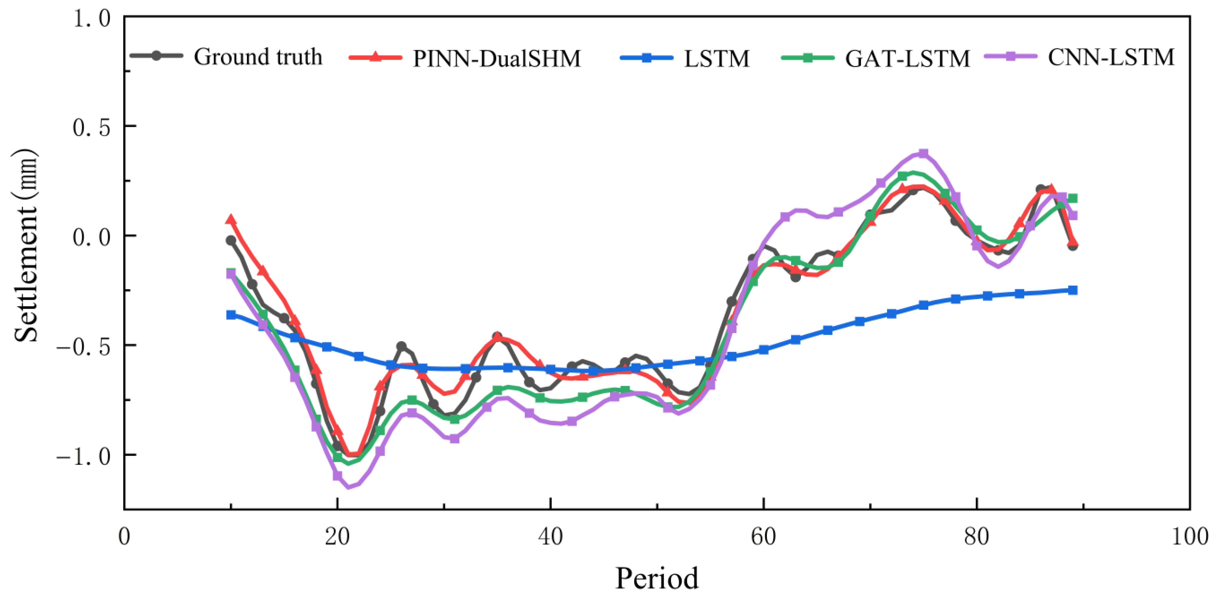
Figure 4 illustrates the comparison between settlement prediction trajectories of various models and actual monitored values on the test set. From the morphology of temporal fitting curves, although the baseline LSTM model captures the general trend of settlement variation, it exhibits noticeable phase lag and amplitude deviation at critical inflection points such as peaks and troughs, reflecting its insufficient capability for decoupling multi-source heterogeneous data. CNN-LSTM and GAT-LSTM demonstrate improvements in overall fitting accuracy but still exhibit oscillations in local nonlinear transition regions. In contrast, PINN-DualSHM’s prediction trajectory demonstrates higher consistency with measured values, maintaining smaller errors during stable phases while exhibiting superior tracking stability during significant fluctuation intervals, indicating that physics-guided and feature decoupling mechanisms facilitate constraint of the solution space and suppression of local noise amplification.

Table 3. Comparison of prediction results for different models.

Model	RMSE (mm)	MAE (mm)	R2	RMSE 95% CI
LSTM	0.281	0.228	0.352	[0.247, 0.313]
CNN-LSTM	0.160	0.145	0.788	[0.146, 0.176]
GAT-LSTM	0.109	0.091	0.901	[0.095, 0.124]
PINN-DualSHM	0.098	0.087	0.925	[0.0946, 0.1014]

quantization results show that PINN-DualSHM performs well in indicators such as RMSE, MAE, and R². Compared with the baseline LSTM, PINN-DualSHM reduces RMSE by 65.12%. Relative to CNN-LSTM and GAT-LSTM, the proposed model decreases the RMSE by 38.75% and 10.09%, while improving the R² by 17.38% and 2.66%, respectively. The research shows that increasing network complexity or adding spatial topology may improve the fitting degree, but there are bottlenecks in cases such as complex dynamic boundaries. Introducing physical constraints and reducing heterogeneous features can better improve the prediction stability and generalization ability under different conditions.

In addition, the coefficient of determination R² of the PINN-DualSHM model reaches 0.925, indicating its reliable capability to explain the overall structural deformation response. The relatively narrow 95% confidence interval of the RMSE, [0.0946, 0.1014], further reflects that the introduction of physical constraints and the heterogeneous feature decoupling mechanism contributes to enhancing predictive stability and generalization capability across different operating conditions. Unlike purely data-driven models, the proposed method embeds the thermodynamic strain superposition principle and settlement monotonicity into the loss function as regularization terms. This mechanism enables the model to fit the data while accommodating key physical priors, thereby reducing the risk of overfitting to a certain extent, decreasing predictive outputs that violate physical laws, and improving the model’s robustness when handling complex conditions such as temperature lag and strain accumulation.

4.4. Statistical Robustness and Significance Analysis of Predictive Performance

To examine the stability of the proposed method under random initialization and sampling conditions, and to objectively evaluate whether its performance difference relative to the baseline models possesses statistical significance, this section conducts an analysis from three dimensions: repeated experiments with multiple random seeds, Bootstrap confidence interval estimation, and significance testing of sample-wise errors.

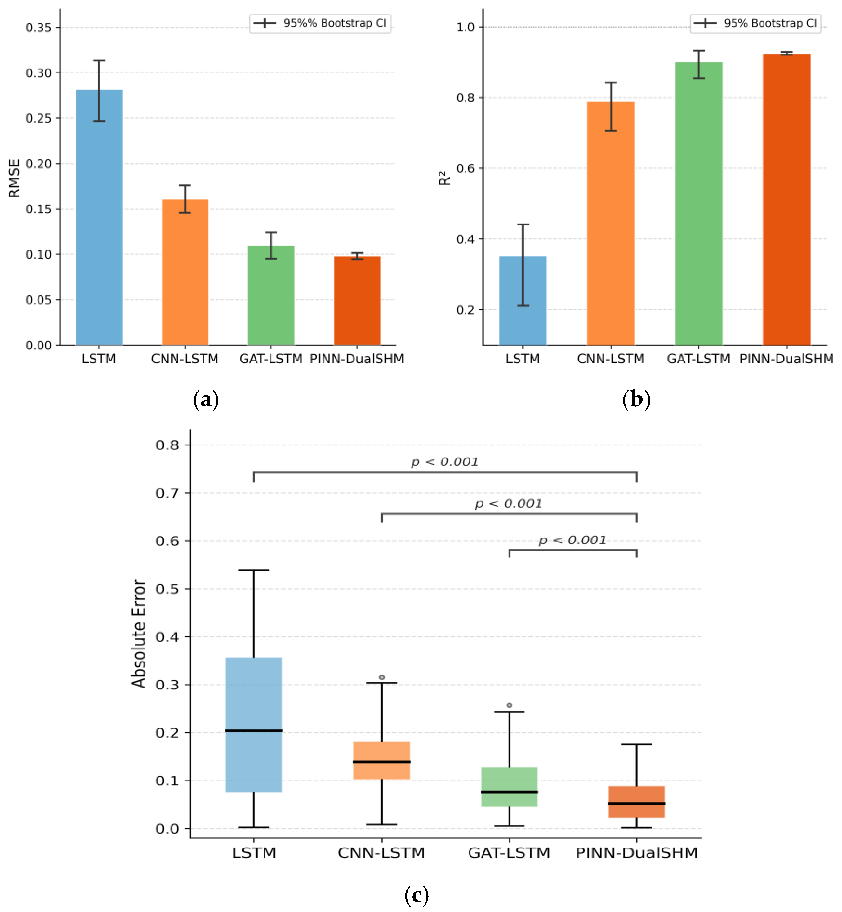
Figure 5a illustrates the Root Mean Square Error (RMSE) of the compared models on the test set. The error bars above the bar charts represent the 95% confidence intervals calculated based on 1000 Bootstrap resampling iterations. The data show that the PINN-DualSHM model achieves a mean RMSE of 0.098, with a 95% confidence interval of [0.0946, 0.1014]. This interval does not overlap with that of the suboptimal model, GAT-LSTM, indicating that the reduction in prediction error achieved by the proposed method is statistically grounded. Similarly, Figure 5b compares the coefficient of determination (R²) of each model. The mean R² of PINN-DualSHM reaches 0.925, with a confidence interval of [0.9209, 0.9291], demonstrating a relatively robust advantage in both data goodness-of-fit and result stability.

Figure 5c presents the distribution of sample-wise absolute errors using box plots. The connecting lines and annotations in the figure reflect the -values of pairwise comparisons between PINN-DualSHM and the baseline models. The test results indicate a significant difference in error distribution between the proposed model and the baseline LSTM and CNN-LSTM models. Furthermore, the comparative conclusion with GAT-LSTM is consistent with the aforementioned phenomenon of non-overlapping confidence intervals. Synthesizing the evaluation results from multiple random seeds and the Bootstrap method, it can be confirmed that the predictive performance of PINN-DualSHM possesses reliable statistical robustness. Its performance improvement relative to the baseline models exhibits significant statistical meaning in terms of RMSE, R², and error distribution.

4.5. Physical Consistency Results and Analysis

In structural health monitoring applications, relying solely on purely statistical error metrics such as RMSE or MAE has inherent limitations. Numerical metrics can only reflect the average degree of fit of a model on an existing dataset; they cannot verify whether the predicted sequence truly follows engineering mechanics principles. If the prediction results exhibit anomalous fluctuations that contradict physical reality (such as severe, irreversible settlement rebound in soft soil foundations), even if the overall error value is extremely low, it will directly compromise the reliability and practical engineering value of the monitoring and early warning system. Therefore, this section conducts an independent evaluation from two dimensions: settlement monotonicity and the temperature-strain coupling mechanism. This step aims to go beyond pure data-driven accuracy assessment and verify the rationality and interpretability of the PINN-DualSHM model outputs at the physical mechanism level.

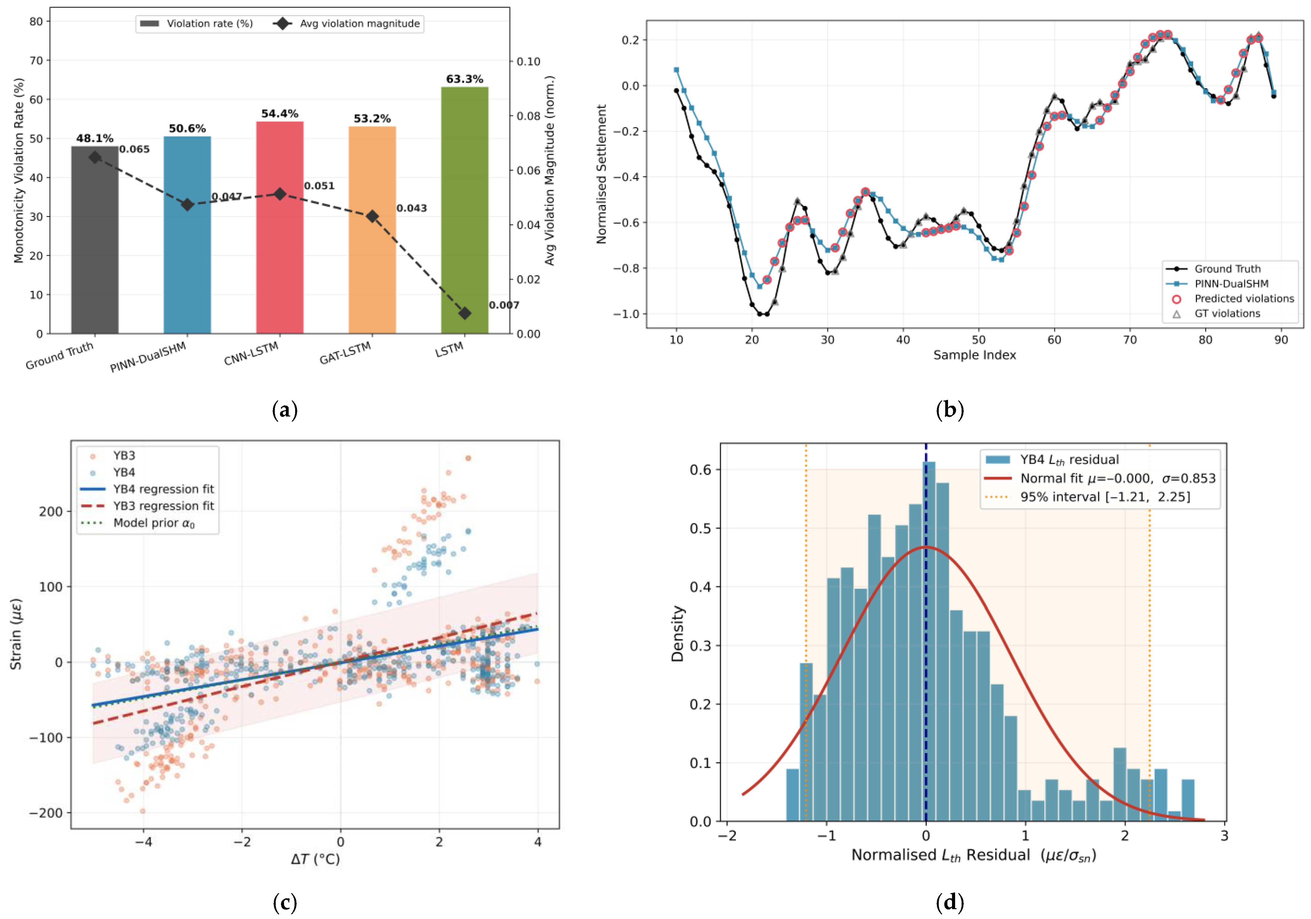
Regarding settlement monotonicity, Figure 6a,b compare the monotonicity violation rate, average violation magnitude, and representative settlement time histories of each model on the test set. The analysis indicates that PINN-DualSHM can effectively suppress abnormal reverse jumps that do not conform to foundation consolidation laws, and its violation rate is closest to the inherent level of the actual monitoring data. Unlike the basic LSTM model, which loses true elastic rebound details due to excessive smoothing, the proposed model accurately retains the short-term reversible deformation that highly coincides with the measured data. This objectively reflects that the monotonicity soft constraint plays a precise screening function in engineering practice: it accommodates reasonable physical fluctuations caused by tides or elastic deformation, while selectively correcting distortions induced by numerical noise.

Regarding the temperature-strain mechanism, Figure 6c,d verify the objective basis of the thermal expansion prior and the strain decomposition assumption. Linear regression results based on the full monitoring data show that the ${\alpha }_{YB3}=1.327\times {10}^{-5}/°\mathrm{C}$ and ${\alpha }_{YB4}=1.119\times {10}^{-5}/°\mathrm{C}$ closely match the physical prior values embedded in the model, demonstrating that the setting of the thermal constraint aligns with the measured environment. Meanwhile, after deducting the thermal expansion component, the distribution of the remaining strain residuals exhibits characteristics of a near-zero mean, a single peak, and no systematic long-term drift. The slightly long right tail of the residuals objectively reveals the true stress state where the structure is prone to generating larger positive additional strains under complex conditions such as heavy traffic loads.

In summary, the physical consistency check confirms the constraining efficacy of prior knowledge from the underlying data level. The introduction of physical constraints does not diminish the numerical fitting accuracy of the model; instead, it circumvents the blindness of black-box models from the perspective of mechanical mechanisms, significantly enhancing the credibility of the prediction results in practical engineering decision-making.

4.6. Uncertainty Quantification Results and Engineering Decision Insights

Following the verification of the model’s predictive accuracy and physical consistency, this section further evaluates the dual uncertainty quantification mechanism of PINN-DualSHM to define the predictive confidence of the model under complex operating conditions, providing a probabilistic basis for safety-critical engineering decisions.

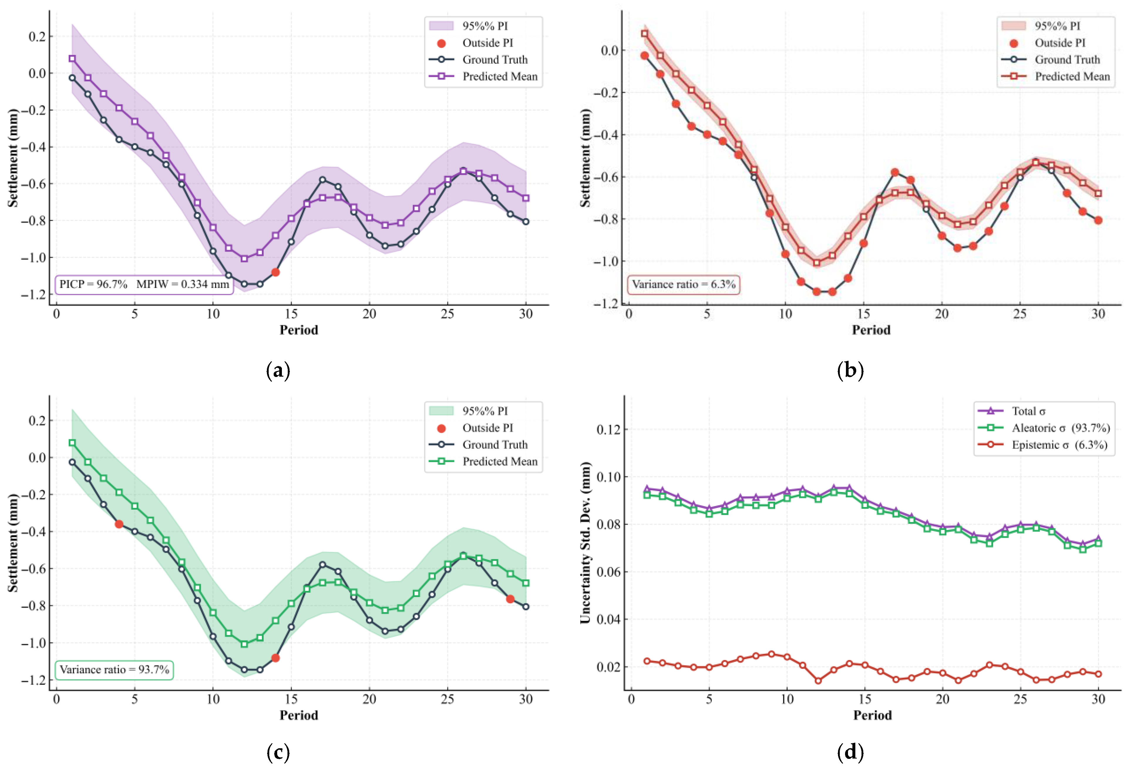
Figure 7a illustrates the 95% prediction interval (PI) formed by the superposition of epistemic and aleatoric uncertainties. The results show that the Prediction Interval Coverage Probability of PINN-DualSHM reaches 96.7%, and the Mean Prediction Interval Width is controlled at 0.334 mm. This width is of the same order of magnitude as the actual fluctuation amplitude of the settlement in the test set, indicating that the prediction interval avoids excessive widening while ensuring high coverage, demonstrating practical engineering applicability. Figure 7b and Figure 7c independently present the 95% intervals corresponding to epistemic uncertainty and aleatoric uncertainty, respectively. A comparison reveals that the epistemic uncertainty interval, which characterizes the stability of model parameters, is relatively narrow, whereas the aleatoric uncertainty interval is wider and envelops the vast majority of the actual observations. The standard deviation evolution curves in Figure 7d further confirm that the total uncertainty is predominantly governed by aleatoric uncertainty (accounting for 93.7%), with the epistemic component remaining at a low level. This decomposition result objectively reflects that after sufficient training and multiple rounds of MC Dropout sampling, the model’s own epistemic bias has been effectively reduced.

The absolute dominance of aleatoric uncertainty indicates that the residual error in the current predictions primarily stems from the inherent, irreducible variability of the data. Specifically, this randomness may originate from short-term disturbances that are not fully modeled, such as sensor measurement noise, sampling errors, and local foundation heterogeneity, as well as missing covariate information in the inputs, such as real-time load distribution or groundwater level fluctuations. It is worth noting that because this study has explicitly constrained structural thermal expansion and consolidation settlement monotonicity through physical priors in the loss function, this residual aleatoric uncertainty more likely reflects objective environmental random disturbances beyond the constraint boundaries, rather than a deficiency in the model’s feature extraction capability.

Synthesizing the above analysis, the quantification design based on heteroscedastic regression and MC Dropout can provide well-calibrated probabilistic interval estimates for settlement prediction. The explicit uncertainty decomposition mechanism enhances the credibility of the black-box model and provides a quantitative reference for subsequent structural state assessment and maintenance risk decision-making.

4.7. Ablation Study

To evaluate the contribution of the core components of PINN-DualSHM to the overall performance, ablation variants are designed for comparison. In

Table 4. Comparison of prediction results under different model configurations.

Test ID	Model Configuration	RMSE (mm)	MAE (mm)	R2
EXP-0	Complete	0.098	0.087	0.925
EXP-1	Removing dual-stream	0.365	0.306	0.810
EXP-2	Removing cross-attention	0.147	0.098	0.895
EXP-3	Removing PINN constraints	0.400	0.340	0.805

, the complete model has the best performance in all indicators: the RMSE is 0.098 mm, the MAE is 0.087 mm, and the R² is 0.925. After removing physical constraints, the dual-branch structure and the adaptive cross-attention mechanism, etc., have performance degradation to different degrees.

Once the physical constraints in the variant are removed, the performance drops significantly. This indicates that physical priors are relatively important for stable generation. Physical constraints limit the space of solutions, enabling predictions to be carried out in accordance with the laws of mechanics and avoiding strange outputs under non-training conditions. When the dual-branch structure is removed, the RMSE increases by 292.48%, which also shows that the decoupled model is necessary for structural response and environmental thermal efficiency. Independently encoding features from different physical mechanisms enhances the feature representation efficiency and generation ability of the model. The performance will also decrease after removing the adaptive cross-attention. This shows that dynamic feature fusion can capture the interaction of multi-source data more than simple concatenation or stacking.

Ablation studies confirm that all three parts, namely physical guidance, time-domain decoupling and adaptive fusion mechanism, must be present.

5. Conclusions

To address the issues of lacking physical interpretability and insufficient generalization capability in structural deformation prediction, this study proposes a physics-informed deep learning framework named PINN-DualSHM. Based on the validation using measured data from an industrial base project in Shenzhen, the following conclusions are drawn:

• By utilizing a dual-branch LSTM encoder and an adaptive cross-attention mechanism, the model effectively separates and extracts structural mechanical responses and environmental thermal effects. Experimental results demonstrate that this mechanism accurately captures temperature lag effects and complex nonlinear deformation trends. The coefficient of determination reaches 0.925, and the predictive accuracy and stability significantly outperform traditional purely data-driven baseline models.
• By embedding the thermodynamic superposition principle and settlement monotonicity into the loss function as regularization terms, the inherent mechanical deficiencies of black-box models are compensated. Physical consistency assessments confirm that this design not only reduces the risk of overfitting but also ensures that the predicted sequences strictly adhere to the objective laws of foundation consolidation and thermal expansion, effectively suppressing anomalous reverse jumps caused by numerical noise.
• Based on heteroscedastic regression and the MC Dropout mechanism, the study reveals that aleatoric uncertainty dominates the total variance (approximately 93.7%). This finding objectively indicates that the current bottleneck in predictive accuracy primarily stems from sensor measurement noise rather than algorithmic logic, providing scientific quantitative support for engineering maintenance strategies prioritized toward “optimizing sensing hardware.”

In summary, the PINN-DualSHM framework achieves a deep integration of physical mechanisms and deep learning advantages, demonstrating significant engineering application prospects for deformation prediction under complex operating conditions. Future research could explore the introduction of nonlinear finite element equations to characterize structural plastic behavior, develop model compression techniques for edge-side deployment, and integrate multi-source monitoring data such as computer vision to further enhance the system’s practicality and interference resistance.

References

1. Fan, G.; Li, J.; Hao, H. Lost data recovery for structural health monitoring based on convolutional neural networks. Struct. Control Health Monit. 2019, 26, e2433. [Google Scholar] [CrossRef]
2. Fan, G.; Li, J.; Hao, H. Dynamic response reconstruction for structural health monitoring using densely connected convolutional networks. Struct. Health Monit. 2021, 20, 1373–1391. [Google Scholar] [CrossRef]
3. Lei, X.M.; Siringoringo, D.M.; Sun, Z.; Fujino, Y. Displacement response estimation of a cable-stayed bridge subjected to various loading conditions with one-dimensional residual convolutional autoencoder method. Struct. Health Monit. 2023, 22, 1790–1806. [Google Scholar] [CrossRef]
4. Li, Y.X.; Ni, P.; Sun, L.M.; Zhu, W. A convolutional neural network-based full-field response reconstruction framework with multitype inputs and outputs. Struct. Control Health Monit. 2022, 29, e2961. [Google Scholar] [CrossRef]
5. Oh, B.K.; Glisic, B.; Kim, Y.; Park, H.S. Convolutional neural network-based data recovery method for structural health monitoring. Struct. Health Monit. 2020, 19, 1821–1838. [Google Scholar] [CrossRef]
6. Oh, B.K.; Park, Y.; Park, H.S. Seismic response prediction method for building structures using convolutional neural network. Struct. Control Health Monit. 2020, 27, e2519. [Google Scholar] [CrossRef]
7. Tang, Z.Y.; Bao, Y.Q.; Li, H. Group sparsity-aware convolutional neural network for continuous missing data recovery of structural health monitoring. Struct. Health Monit. 2021, 20, 1738–1759. [Google Scholar] [CrossRef]
8. Wu, R.T.; Jahanshahi, M.R. Deep Convolutional Neural Network for Structural Dynamic Response Estimation and System Identification. J. Eng. Mech. 2019, 145, 04018125. [Google Scholar] [CrossRef]
9. Fan, G.; He, Z.Y.; Li, J. Structural dynamic response reconstruction using self-attention enhanced generative adversarial networks. Eng. Struct. 2023, 276, 115334. [Google Scholar] [CrossRef]
10. Fan, G.; Li, J.; Hao, H.; Xin, Y. Data driven structural dynamic response reconstruction using segment based generative adversarial networks. Eng. Struct. 2021, 234, 111970. [Google Scholar] [CrossRef]
11. Lei, X.M.; Sun, L.M.; Xia, Y. Lost data reconstruction for structural health monitoring using deep convolutional generative adversarial networks. Struct. Health Monit. 2021, 20, 2069–2087. [Google Scholar] [CrossRef]
12. Duan, D.Y.; Wang, Z.C.; Sun, X.T.; Xin, Y. A data fusion method for bridge displacement reconstruction based on LSTM networks. Smart Struct. Syst. 2022, 29, 599–616. [Google Scholar]
13. Zhang, Z.; Sun, C. Structural damage identification via physics-guided machine learning: A methodology integrating pattern recognition with finite element model updating. Struct. Health Monit. 2021, 20, 1675–1688. [Google Scholar] [CrossRef]
14. Raissi, M.; Perdikaris, P.; Karniadakis, G.E. Physics-informed neural networks: A deep learning framework for solving forward and inverse problems involving nonlinear partial differential equations. J. Comput. Phys. 2019, 378, 686–707. [Google Scholar] [CrossRef]
15. Haywood-Alexander, M.; Bacsa, K.; Liu, W.; Lai, Z.; Chatzi, E. Physics Enhanced Machine Learning for Monitoring and Twinning. Struct. Health Monit. 2023. [Google Scholar] [CrossRef]
16. Liu, W.; Lai, Z.; Bacsa, K.; Chatzi, E. Physics-guided deep markov models for learning nonlinear dynamical systems with uncertainty. Mech. Syst. Signal Process. 2022, 178, 109276. [Google Scholar] [CrossRef]
17. Lai, Z.; Mylonas, C.; Nagarajaiah, S.; Chatzi, E. Structural identification with physics-informed neural ordinary differential equations. J. Sound. Vib. 2021, 508, 116196. [Google Scholar] [CrossRef]
18. Cianci, E.; Civera, M.; De Biagi, V.; Chiaia, B. Predictive Modelling of bridge bearing displacements with Physics-Enhanced Machine Learning (PEML) environmental effects filtering. ce/papers 2025, 8, 156–163. [Google Scholar] [CrossRef]
19. Cianci, E.; Civera, M.; De Biagi, V.; Chiaia, B. Physics-informed machine learning for the structural health monitoring and early warning of a long highway viaduct with displacement transducers. Mech. Syst. Signal Process. 2026, 242, 113659. [Google Scholar] [CrossRef]
20. Kendall, A.; Gal, Y. What uncertainties do we need in bayesian deep learning for computer vision? Adv. Neural Inf. Process. Syst. 2017, 30, 5580–5590. [Google Scholar]
21. Hochreiter, S.; Schmidhuber, J. Long short-term memory. Neural Comput. 1997, 9, 1735–1780. [Google Scholar] [CrossRef]
22. Rossi, R.A.; Zhou, R.; Ahmed, N.K. Deep Inductive Graph Representation Learning. IEEE Trans. Knowl. Data Eng. 2020, 32, 438–452. [Google Scholar] [CrossRef]
23. Huo, J.; Liu, S.; Zhang, Z.; Liu, Q. Multi-Scale Long-Short Term Memory Neural Network Method for Predicting Wind Pressure on Coal Shed Surface. Eng. Mech. 2024, 41, 179–186. [Google Scholar]
24. Chen, X. Prediction of Building Settlement Induced by Tunnel Excavation Using TimeGAN and LSTM Neural Network. S. China J. Seismol. 2022, 42, 107–115. [Google Scholar]
25. Zhang, W. Structural Integrity Management of Offshore Engineering Based on the Value of Health Monitoring Information. Harbin Inst. Technol. 2024, 8. [Google Scholar] [CrossRef]
26. Hüllermeier, E.; Waegeman, W. Aleatoric and epistemic uncertainty in machine learning: An introduction to concepts and methods. Mach. Learn. 2021, 110, 457–506. [Google Scholar] [CrossRef]
Figure 1. Internal architecture of LSTM cell.
Applsci 16 03194 g001
Figure 2. Architecture of the PINN-DualSHM hybrid model.
Applsci 16 03194 g002
Figure 3. On-site equipment installation diagram. (a) Settlement monitoring points; (b) Strain monitoring points.
Applsci 16 03194 g003
Figure 4. Prediction results of different models.
Applsci 16 03194 g004
Figure 5. Evaluation results. (a) Comparison of RMSE metrics across models; (b) Comparison of R2 across models; (c) Sample-wise absolute error distributions and significance tests.
Applsci 16 03194 g005
Figure 6. Physical constraint diagnostics. (a) Monotonicity violation rate versus violation magnitude; (b) Time series tracking of monotonicity; (c) Temperature-strain scatter and regression plot; (d) Temperature-strain residual distribution.
Applsci 16 03194 g006
Figure 7. Uncertainty quantification results. (a) Total uncertainty; (b) Epistemic uncertainty; (c) Aleatoric uncertainty; (d) Decomposition comparison.
Applsci 16 03194 g007