Surface Morphology Effects on Turbulent Structure and Diffusion Across Multiple Underlying Surfaces in a Wind Tunnel

Abstract

Turbulent structure and diffusion over different underlying surfaces are fundamental to understanding mass and momentum exchange in the atmospheric boundary layer. This study investigated these processes over six distinct surfaces—flat plate, sand, grass, small gravel, large gravel, and vegetation—through wind tunnel experiments combined with high-frequency velocity measurements. Quadrant analysis, Reynolds stress decomposition, and turbulence kinetic energy budget analysis were employed to elucidate the mechanisms driving variations in diffusion coefficients. The results reveal two distinct turbulence generation regimes: over rigid surfaces (flat plate, sand, gravel), turbulence is primarily generated by roughness elements, whereas over canopy surfaces (grass, vegetation), canopy-induced shear and wake dynamics dominate. Consequently, the vertical profiles of turbulent diffusion coefficients K_x and K_z exhibit markedly different patterns across surface types. For rigid surfaces, diffusion coefficients peak near the surface and decay monotonically with height. For canopy surfaces, diffusion coefficients reach their maximum at the canopy top, reflecting the dual influence of canopy-induced shear and energy dissipation within the canopy. These findings provide a mechanistic understanding of surface-induced variability in turbulent diffusion processes and offer quantitative parameterizations that can improve pollutant dispersion modeling over complex terrain.

1. Introduction

The exchange of momentum and scalars in the atmospheric boundary layer (ABL) is profoundly influenced by underlying surface conditions. Numerous studies have shown that the turbulent structure of the near-surface flow field depends on surface roughness and topographic features. Over flat and smooth surfaces, turbulence generally follows classical, well-organized behavior, whereas above rough surfaces (such as urban areas or forest canopies), the turbulent structure is more complex and remains incompletely understood. These observational phenomena indicate that turbulent characteristics exhibit significant differences across various surface types, particularly in terms of turbulent transport, momentum transport, and the turbulent kinetic energy (TKE) budget. As turbulent diffusion is one of the primary mechanisms for pollutant dispersion in the atmosphere, these differences substantially influence turbulent diffusion within the ABL. Investigating the turbulent characteristics and structures in different types of boundary layers contributes to understanding the patterns of turbulent diffusion and transport properties in these layers, offering important theoretical significance and practical value for improving the simulation and prediction of pollutant dispersion and transport processes in the atmospheric environment.

Numerous studies have systematically explored the turbulent characteristics over different types of underlying surfaces. Research using classical wind tunnels, numerical simulations, and field experiments has revealed notable differences in turbulent transport between smooth and rough surfaces. Stiperski et al. [1] compared turbulent flows over complex terrain with those over flat and horizontally homogeneous terrain, finding significant anisotropy in turbulence over complex topography. Their scaling analysis demonstrated considerable deviations from the empirical formulas developed for flat, uniform terrain. Raoni et al. [2] conducted a study in the Amazon region, comparing dense forests (rough surfaces) against water surfaces (smooth surfaces). Their research revealed significant differences between these two surface types in terms of turbulence intensity, power spectra, and the temporal and length scales of eddies, as well as the primary terms in the TKE budget. These studies confirm that turbulent characteristics vary significantly across different surface types, particularly in turbulent transport, momentum transport, and the TKE budget. Keirsbulck et al. [3] examined turbulent boundary layers over smooth surfaces and rough walls, identifying fundamental structural differences between them. Lee and Sung [4] performed the direct numerical simulation (DNS) of a turbulent boundary layer (TBL) over rough and smooth walls, demonstrating that surface roughness alters turbulent stresses in both the roughness sublayer and the outer layer, thereby significantly impacting vertical turbulent transport throughout the entire TBL. Lee et al. [5] employed DNS to study TBL characteristics over cubical roughness elements and compared them with two-dimensional rod-roughened walls. Their results indicated that surface roughness substantially alters turbulent flows, not only modifying near-wall streak structures, but also restructuring hairpin vortex packets in the outer layer and significantly impacting Reynolds stresses throughout the boundary layer. However, the dimensional differences between 2D and 3D roughness had negligible effects on turbulent statistics and coherent structures. Mejia-Alvarez and Christensen [6] used PIV wind tunnel experiments to investigate flow characteristics in the roughness sublayer over highly irregular rough surfaces. Their research showed that roughness redistributes TKE and can promote TKE generation in preferred regions within the roughness sublayer. They also observed that the rough-wall flows exhibit significant spanwise local heterogeneity in the contributions of ejections and sweeps compared to smooth walls. Hwang and Lee [7] conducted DNS to analyze the TBL over streamwise-aligned surface roughness, exploring the effects of roughness on mean flow properties associated with counter-rotating large secondary flows. They found that the active transport of kinetic energy induced by ridge roughness edges closely correlates with the upward deflection of spanwise motions from the valley floor. Furthermore, Christen et al. [8] found that, in the urban roughness sublayer, the presence of buildings leads to TKE production, redistribution, and dissipation processes that distinctly differ from those over flat surfaces.

In terms of momentum transport, which describes the transfer of momentum within fluid and represents a critical aspect of turbulence, quadrant analysis serves as a common statistical method in turbulence research. This technique is used to identify and quantify the contributions of turbulent shear stress (Reynolds stress), particularly those from coherent vortex structures associated with momentum transport. Perry and Schofield [9] proposed a model based on the concept of coherent vortex structures to describe the mean velocity and shear stress distributions in turbulent boundary layers. This model decomposed the boundary layer into two distinct regions and introduced the concept of “A-vortices” to explain the turbulent structure. Shaw et al. [10] identified a fundamental difference in momentum transport mechanisms between smooth and rough walls. Their work demonstrated that momentum transport near smooth walls is dominated by outward ejection events (Quadrant Q2), whereas near rough walls, it is governed by downward sweep events (Quadrant Q4). Subsequent field observations in vegetation canopies corroborated this pattern, revealing that momentum input within the canopy primarily originates from high-momentum sweep events from above, while transport at higher levels above the canopy shifts to being dominated by ejections. Mauree et al. [11] investigated urban environments and found that building height and arrangement significantly alter momentum flux. Their research concluded that momentum transport within the urban canopy is far more complex than over flat terrain, with surface roughness playing a decisive role. Baldocchi and Meyers [12] contrasted momentum transport over smooth and rough surfaces, finding that the lower resistance of smooth surfaces leads to inefficient momentum transport. In contrast, within rough surfaces such as forest canopies, the complex structure modifies wind profiles and turbulence intensity, leading to momentum transport characteristics that differ from those measured in the surface boundary layer over flat terrain. Dixit et al. [13] investigated the universality of wall-scaling in zero-pressure-gradient turbulent boundary layers. Their study highlighted the role of TKE production, which represents the kinetic energy transfer from the mean flow to large turbulent eddies. This process signifies the conversion of momentum from the mean flow to turbulent motion, with shear effects near solid surfaces being a key mechanism for generating TKE. Desai et al. [14] further emphasized the distinctive turbulent characteristics within forest canopies compared to measurements in open sections of the atmospheric boundary layer. Their work attributed these differences to the modification of wind profiles and turbulence intensity by dense vegetation, which subsequently alters momentum transport processes. The turbulent kinetic energy budget equation encompasses production, dissipation, transport, and buoyancy terms, which collectively govern the spatial and temporal distribution of TKE. Rogachevskii et al. [15] elaborated on the development and application of the energy flux budget (EFB) turbulence closure theory in the surface layer under both convective and stably stratified atmospheric conditions. The study demonstrated that the TKE production term is closely linked to shear from the mean flow, which converts energy from the mean motion into turbulent kinetic energy. This conversion represents the key mechanism for transferring momentum from the mean flow to large turbulent eddies.

Wei [16] investigated the integral properties of TKE production and dissipation in zero-pressure-gradient turbulent boundary layers (ZPG TBLs) using DNS and high-resolution experimental data. The research identified three key findings: the connection between the mesoscale length and the peak location of Reynolds shear stress; the near-equal partitioning of integrated TKE production and dissipation at that specific location; and the variation in integral properties of TKE production and dissipation with the Reynolds number. Cindori et al. [17] compared TKE production over smooth and rough surfaces and found that TKE production relies primarily on mean shear and remains relatively low in magnitude on smooth surfaces. In contrast, TKE production intensifies significantly with increasing roughness elements over rough surfaces. Studies on the urban roughness sublayer have shown that the magnitude and distribution of all TKE budget terms, including production, dissipation, and transport, are influenced by building geometry, creating marked differences from those over flat terrain [18]. From forest canopy studies, Babić and Rotach [19] concluded that, given the substantial surface resistance and pronounced wind shear on highly rough surfaces, the shear production term typically serves as the primary source of TKE. Tian and Conan [20] employed large eddy simulation (LES) to conduct a detailed three-dimensional analysis of turbulence generation within an urban canopy. Significant regions of both positive and negative turbulence production were identified close to the ground, which were associated with distinct features of the mean flow.

The aforementioned research demonstrates that canopies and rough surfaces significantly influence turbulent transport, momentum transport, and the TKE budget within the boundary layer. Turbulent diffusion, the process driven by turbulent motions that transports mass, energy, or momentum, is directly affected by underlying surface conditions that alter its characteristics and distribution patterns in the boundary layer. Considerable research has been conducted to investigate the turbulent diffusion characteristics over canopies and rough surfaces. For instance, Ukequchi et al. [21] investigated turbulent diffusion by measuring wind speed and turbulent velocity to determine the turbulent diffusion coefficient. Their experiments revealed that the coefficient reaches the maximum at a certain height and subsequently decreases to a much smaller value under uniform flow conditions. Ohya and Sekishita [22,23] separately conducted wind tunnel experiments to investigate atmospheric boundary layers with different surface roughness and turbulent characteristics. Mouri et al. [24] performed wind tunnel experiments to examine turbulent diffusion from small surface sources into the boundary layer. Kanda and Su et al. [25,26] conducted a pioneering large-eddy simulation (LES) of flow through forest canopies. Their previous work successfully captured key features of canopy-induced turbulence and clarified essential modeling requirements and appropriate simulation forcing parameters. Yue et al. [27] developed an improved diffusion model by incorporating a drag model that accounts for resistance from plant trunks.

Considerable research has been conducted on the turbulent structures over rough surfaces and canopies, and the turbulent diffusion characteristics over rough surfaces and vegetation canopies have also been extensively studied. However, due to the significant differences in turbulence generation mechanisms between rough surfaces and canopies, studies analyzing these mechanistic differences across various rough surfaces and canopy types remain limited. A research gap persists in linking the vertical distribution of turbulent diffusion characteristics to surface properties, underscoring the need for an integrated analysis combining turbulent structures with diffusion characteristics across different surface types.

To address this research gap, in this study, the turbulent characteristics of atmospheric boundary layers over various underlying surfaces are systematically investigated through wind tunnel experiments. Six surfaces were designed: flat plate, sand surface, small gravel surface, larger gravel surface, grass surface, and vegetation model. A two-dimensional hot-wire anemometer was employed to measure streamwise and vertical fluctuating velocities under various Reynolds number conditions. By elucidating the mechanistic links between turbulent diffusion and turbulent structures through the analysis of turbulent quadrants and TKE budget terms, this work provides insights and theoretical foundations for developing empirical formulas and models of turbulent diffusion coefficients over distinct types of underlying surfaces.

2. Experimental Setup

The experiments were conducted in a direct-flow, low-turbulence wind tunnel with a test section measuring 5 m in length and 0.6 m × 0.6 m in cross-section. Six sets of homogeneous surfaces were fabricated: flat plate, sand surface, small gravel, large gravel, grass, and vegetation. High-frequency wind velocity data at various heights over each surface were acquired using a Hanghua CAT-04 Constant Temperature Anemometry (Dalian HangHua Technology Co., Ltd., Dalian, China). The two-dimensional hot-wire system consists of a 2D hot-wire probe, a data acquisition unit, a mainframe computer, and a CR04 hot-wire anemometer calibrator. In this study, a single X-type 2D hot-wire probe was used for the experiments. The temperature difference between calibration and measurement was maintained within ±1°. The CR04 hot-wire anemometer calibrator (Dalian HangHua Technology Co., Ltd., Dalian, China) is a jet device capable of delivering a set outlet velocity. Its jet nozzle has a diameter of 1.0 cm and produces a steady flow field with velocities ranging from 1 to 60 m/s. The turbulence intensity is below 0.5%. The yaw angle range is ±45°, and the rotation angle covers 0–360. Before the experiments, the hot-wire probe was calibrated using the CR04 calibrator. By adjusting the probe’s cold-resistance Ohms, overheat ratio, and balance parameter, the square-wave characteristic time of the probe was set to approximately 4.3 μs. A fourth-order polynomial function was employed for velocity fitting during calibration.

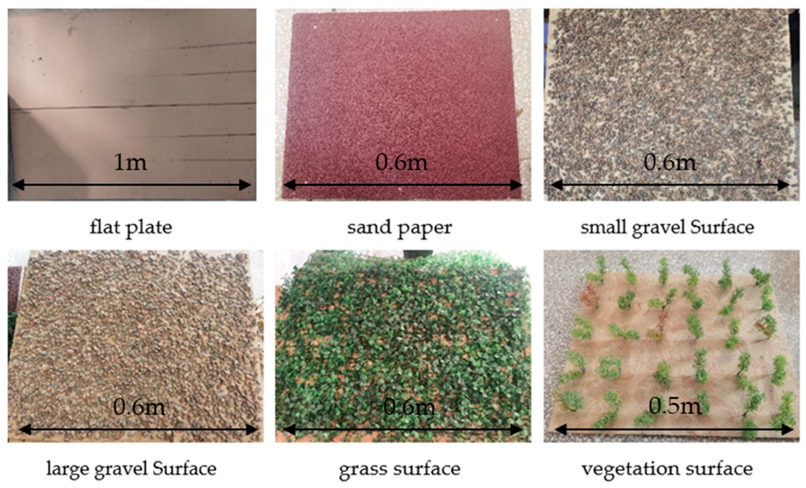
Figure 1 shows physical images of the six fabricated surfaces. The manufacturing and installation methods for each surface are described below.

Flat Plate: Five smooth plates (0.6 m × 1 m × 0.01 m) were cut and connected using fasteners within the wind tunnel to form a continuous, level surface throughout the test section.

Sand Surface: Forty-six grit sandpaper sheets (0.6 m × 0.5 m) were adhered to plates of identical dimensions using glue and secured with self-tapping screws, ensuring firm bonding and a flush surface across the test section.

Gravel Surface: White latex adhesive was evenly applied to plates (0.6 m × 0.5 m × 0.01 m). Washed and dried gravel was spread over the adhesive and compacted to achieve uniform coverage. Ten plates each were prepared using gravel with median diameters of 2 mm (small gravel) and 4 mm (large gravel).

Grass Surface: Artificial turf mats (0.6 m × 0.5 m × 0.01 m) were anchored at each corner to underlying plates of the same size. Turf at the junctions between plates was trimmed to ensure seamless continuity and surface evenness. The height of the artificial turf was approximately 30 mm.

Vegetation Surface: Plates (0.6 m × 0.5 m × 0.01 m) were drilled with 30 equally spaced holes (streamwise spacing: 0.1 m, spanwise spacing: 0.1 m). Artificial vegetation elements, approximately 0.08 m in height, were inserted into the holes.

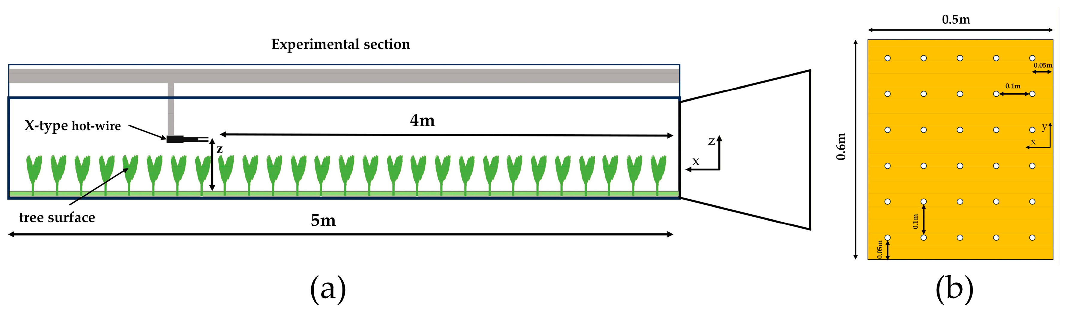
Figure 2a shows the layout of the vegetation surface in the wind tunnel experiment. The vegetation distribution is illustrated in Figure 2b. A single two-component hot-wire anemometer was positioned 4 m downstream from the test section inlet to measure high-frequency streamwise (u) and vertical ($w$) wind velocity data at various heights above each surface. Measurements were acquired at a sampling frequency of 5000 Hz, with each height level recorded for 2 min and repeated three times. Due to the gaps between the model vegetation elements, high-frequency wind velocity data were measured within the vegetation canopy for that surface. In contrast, the artificial turf of the grass surface was relatively dense, allowing measurements only above the turf layer. For all surfaces, the flat plate surface was used as the reference no-slip condition for fitting the boundary-layer wind profiles. This approach facilitates a more consistent comparison of how turbulent parameters vary with height across the different surfaces.

The mean streamwise wind velocity profiles at different heights were determined from wind tunnel experiments for each underlying surface type at varying Reynolds numbers, with measurements performed using a two-dimensional hot-wire anemometer. Based on the vertical distribution characteristics of the streamwise velocity, the flow field can be divided into the boundary layer region and the free-stream region. The boundary layer region exhibits a logarithmic velocity profile, whereas the free-stream region lies above the boundary layer. By fitting the logarithmic wind profiles, the friction velocity (u*) and aerodynamic roughness length (z₀) were determined for each surface under various Reynolds numbers. The boundary layer height (δ) was derived by substituting 0.99U_∞ into the logarithmic profile equation, where U_∞ represents the average wind velocity in the free-stream region. The Reynolds number and logarithmic profile equations are given as follows:

$$\mathit{Re}={\displaystyle \frac{{\rho U}_{\infty }D}{\mu }}$$

(1)

$$u\left(z\right)={\displaystyle \frac{u^{\ast }}{\kappa }}ln\left({\displaystyle \frac{z}{z_0}}\right)$$

(2)

The experimental parameters are defined as follows: ρ is the air density; U_∞ is the free-stream velocity; D is the characteristic length, defined as the wind tunnel height (D = 0.6 m); and μ is the dynamic viscosity of air, where u(z) represents the streamwise velocity at height z; u* is the friction velocity; κ is the von Kármán constant (typically taken as 0.41); z is the measurement height; and z₀ is the aerodynamic roughness length.

To compare the differences in flow characteristics within the boundary layer under various surface conditions, the measurement height z is non-dimensionalized relative to the corresponding boundary layer height δ under each operating condition, and is defined as the normalized height ζ = z/δ.

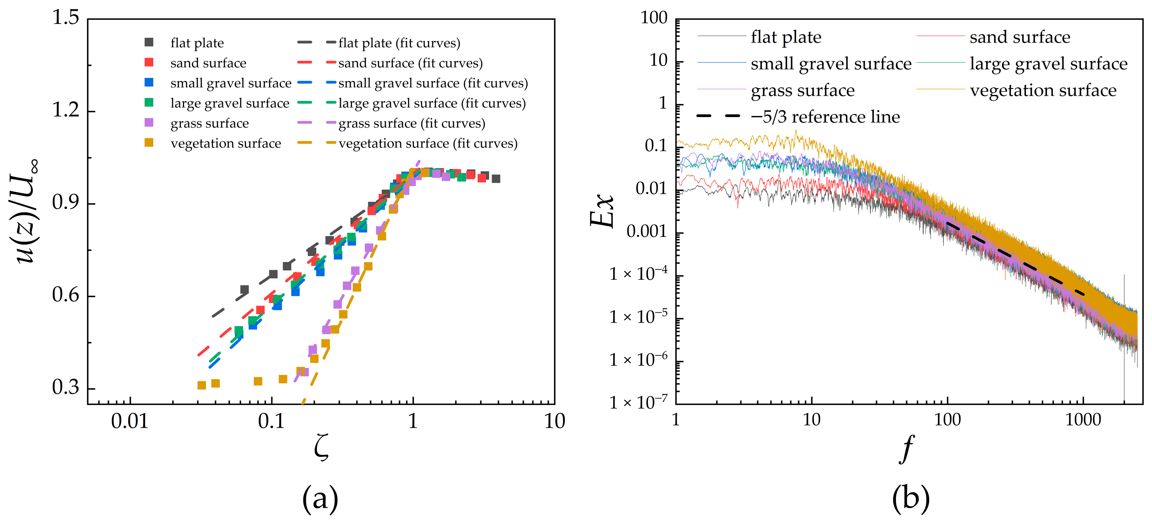
The normalized wind velocity profiles for each surface are shown in Figure 3a, where the vertical and horizontal axes represent the normalized wind velocity and normalized height, respectively. The non-dimensional velocity profile u(z)/U_∞ primarily depends on ζ and is independent of the absolute scale. This approach eliminates the scaling effects caused by differences in boundary layer thickness δ due to Reynolds number or surface roughness. The solid lines in the figure represent the fitted velocity profiles for each surface. It can be observed that the wind speed profiles near the boundary of each surface follow the logarithmic law, indicating the formation of a stable boundary layer. In this experiment, wind velocity profiles were measured at multiple streamwise locations for each surface. By a downstream distance of 2.8 m, the boundary layer velocity profiles were fully developed. To validate the reliability of the hot-wire measurements, the streamwise velocity data at a selected height within the boundary layer for each surface were processed using Fast Fourier Transform (FFT) to obtain the streamwise velocity spectra (Ex) at ζ ≈ 0.5. As shown in Figure 3b, where the vertical and horizontal axes represent Ex and frequency ƒ, respectively, the spectra for all surfaces follow the −5/3 scaling law in the frequency range of 100–500 Hz. This confirms that the sampling frequency of 5000 Hz was sufficient to capture the turbulent characteristics of the different surfaces.

The specific Re values for each surface type and test condition are listed in

Table 1. Boundary layer parameters of various underlying surfaces (friction wind speed u*, surface roughness z₀, and boundary layer height L).

u*
Underlying Surfaces	Re
	2.05 × 105	2.47 × 105	3.29 × 105	4.11 × 105	4.93 × 105
Flat plate	0.31745	0.4038	0.49194	0.64871	0.78216
Sand surface	0.42341	0.56103	0.69474	0.92387	0.95724
Small gravel surface	0.44726	0.57137	0.71204	0.90907	1.10807
Large gravel surface	0.51205	0.60197	0.70963	0.87464	1.01042
Grass surface	0.93813	1.21374	1.53541	1.91766	2.06822
Vegetation surface	1.14073	1.4450	1.76971	2.21168	2.55601
z0 (mm)
Underlying surfaces	Re
	2.05 × 105	2.47 × 105	3.29 × 105	4.11 × 105	4.93 × 105
Flat plate	0.07516	0.07221	0.05882	0.0726	0.06414
Sand surface	0.47568	0.51319	0.49094	0.61341	0.26365
Small gravel surface	0.88618	0.77654	0.68773	0.65582	0.68368
Large gravel surface	1.30151	0.89108	0.7525	0.67774	0.58672
Grass surface	15.27931	15.44486	15.55442	15.02164	11.92955
Vegetation surface	26.82192	25.43766	24.49781	23.91194	22.94488
δ (mm)
Underlying surfaces	Re
	2.05 × 105	2.47 × 105	3.29 × 105	4.11 × 105	4.93 × 105
Flat plate	73.9	72.3	74.7	82.1	77.9
Sand surface	98.7	96.2	101.1	105.8	98.4
Small gravel surface	131.2	129.8	132.8	130.3	136.0
Large gravel surface	136.3	127.2	138.5	136.5	137.0
Grass surface	177.5	187.7	188.9	191.3	203
Vegetation surface	247.5	249.2	251.2	252	250.1

. The experiment encompassed six different surfaces. For each surface, measurements were conducted at five different Reynolds numbers, resulting in a total of 30 test cases.

Table 1 presents the fitting parameters u*, z₀, and δ obtained from logarithmic velocity profiles under different wind speeds. The friction velocity u* increases monotonically with Re for all surfaces and, at a fixed Re, is larger over rougher surfaces—a trend that aligns with the classical boundary layer prediction of increasing wall shear stress with flow velocity. Notably, the increase in u* is most pronounced for the flat plate (146%), while the grass and vegetation surfaces, despite having the highest absolute u* values, show a smaller increase (120%). This reflects distinct turbulence generation mechanisms: flat plate turbulence arises from viscous sublayer instabilities, whereas canopy turbulence is driven by foliar disturbance of the flow field.

The roughness length z₀ exhibits nonlinear Re dependence: for low-roughness surfaces (flat plate, sand surface), z₀ remains stable; for high-roughness surfaces (gravel surface, grass surface, vegetation surface), z₀ decreases slightly with increasing Re. The z₀ values for grass surface (10–15 mm) and vegetation surface (22–27 mm) are an order of magnitude higher than for other surfaces. Under dense canopy conditions, z₀ reaches 40–50% of the actual vegetation height (e.g., z₀ ≈ 12–15 mm for grass surface), consistent with forest canopy observations and validating z₀ as a descriptor of surface geometry.

Boundary layer height δ decreases in the following order: vegetation > grass > large gravel > small gravel > sand surface > flat plate. The δ for grass (177.5–203.0 mm) is 2.5 times that of the flat plate (72.3–82.1 mm), consistent with roughness-enhanced turbulent mixing. For vegetation, δ ≈ 250 mm, which approaches half of the wind tunnel height (300 mm), limiting Re-induced variation. Regarding Re effects, δ increases with Re for all surfaces but with different growth rates: the flat plate shows only a 4.1% increase, conforming to smooth-wall theory, while grassland exhibits a 14% increase, reflecting the Re-dependent nature of canopy turbulence.

For comparing parameters across different surfaces at non-dimensional heights, the surface of the wooden plate is defined as the zero-displacement plane. The grass canopy is relatively dense, with its top at approximately ζ ≈ 0.14. The vegetation canopy has spacing between its elements, and due to swaying during the experiment, its top height is considered to be within ζ ≈ 0.28–0.32.

3. Results

By analyzing the high-frequency wind velocity data from the six surfaces, we obtained the probability density distributions of streamwise and vertical velocity fluctuations, quadrant distributions, and the variation in turbulent production and dissipation rate with height for each surface (flat plate, sand surface, grass, small gravel, large gravel, and vegetation). These results were used to analyze the influence of different turbulent structures on the turbulent diffusion coefficients.

3.1. Normalized Velocity Fluctuations

Parameters such as boundary layer height and turbulence intensity vary significantly across surfaces due to factors like surface roughness. This prevents the direct comparison of quadrant distribution characteristics using raw velocity fluctuations. The friction velocity u* serves as a characteristic velocity scale that directly reflects the magnitude of shear stress (i.e., momentum exchange intensity) within the flow. The streamwise (u′) and vertical ($w$′) velocity fluctuations were normalized using u*. 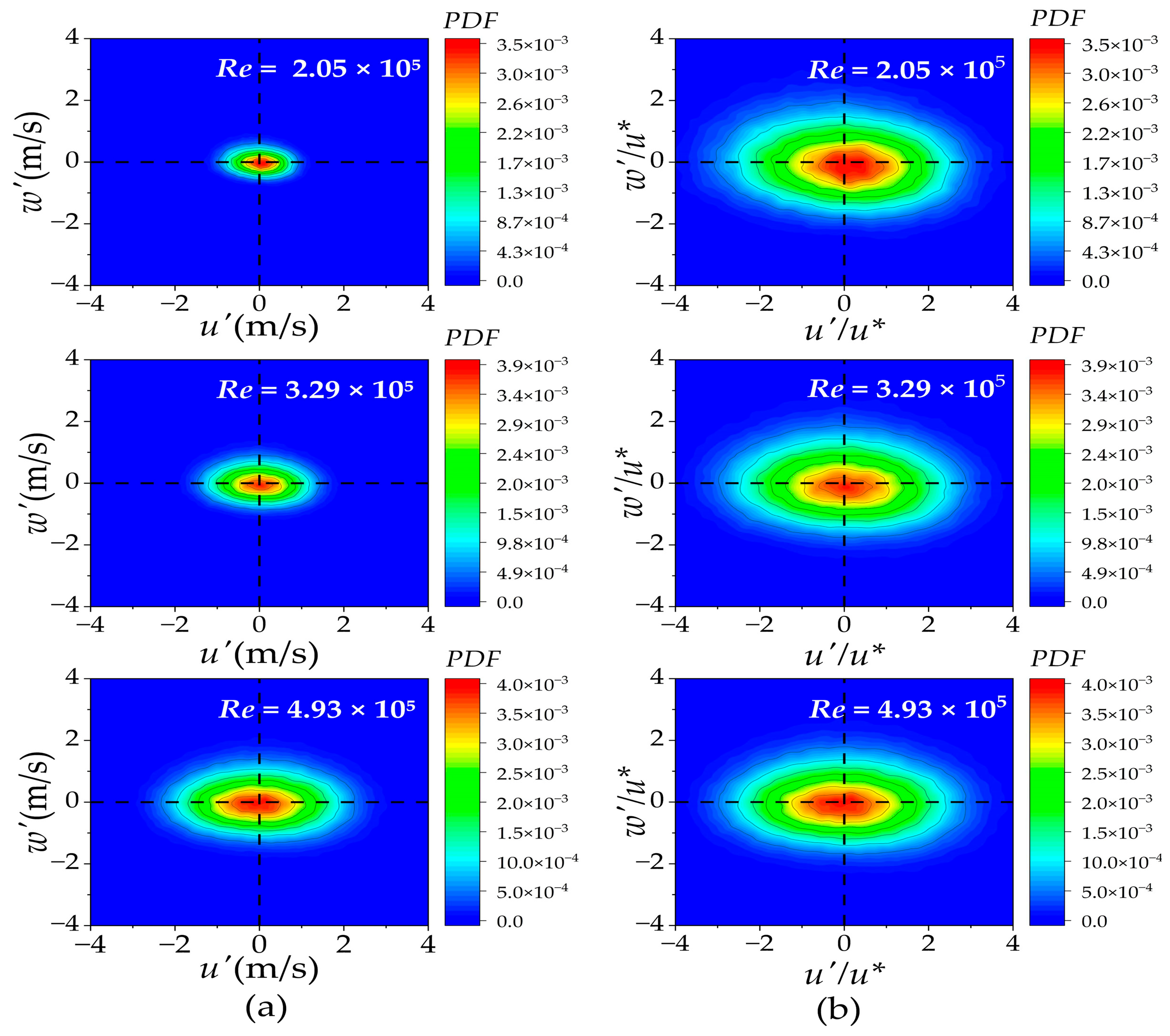Figure 4 presents the probability density distributions of both the normalized and raw velocity fluctuations at the same height over the flat plate.

As shown in Figure 4, the probability density distributions of both velocity fluctuation components over the flat plate surface approximate an elliptical shape, with relatively uniform scatter across the four quadrants. The comparison of different Reynolds numbers (rows in Figure 4) reveals that while the shape of the probability density distribution remains largely consistent at the same height, the magnitude of the velocity fluctuations increases with the Reynolds number. In contrast, the shape and magnitude of the normalized velocity fluctuations show minimal variation. In summary, the normalized velocity fluctuations directly represent the local fluctuation intensity relative to the wall-driven forcing, thereby linking the raw velocity fluctuations to the wall shear stress, which is the fundamental mechanism responsible for generating turbulence. Normalizing the raw fluctuations by the wall shear stress enables the comparative analysis of the probability density distributions across different surfaces.

3.2. Quadrant Distributions of Different Underlying Surfaces

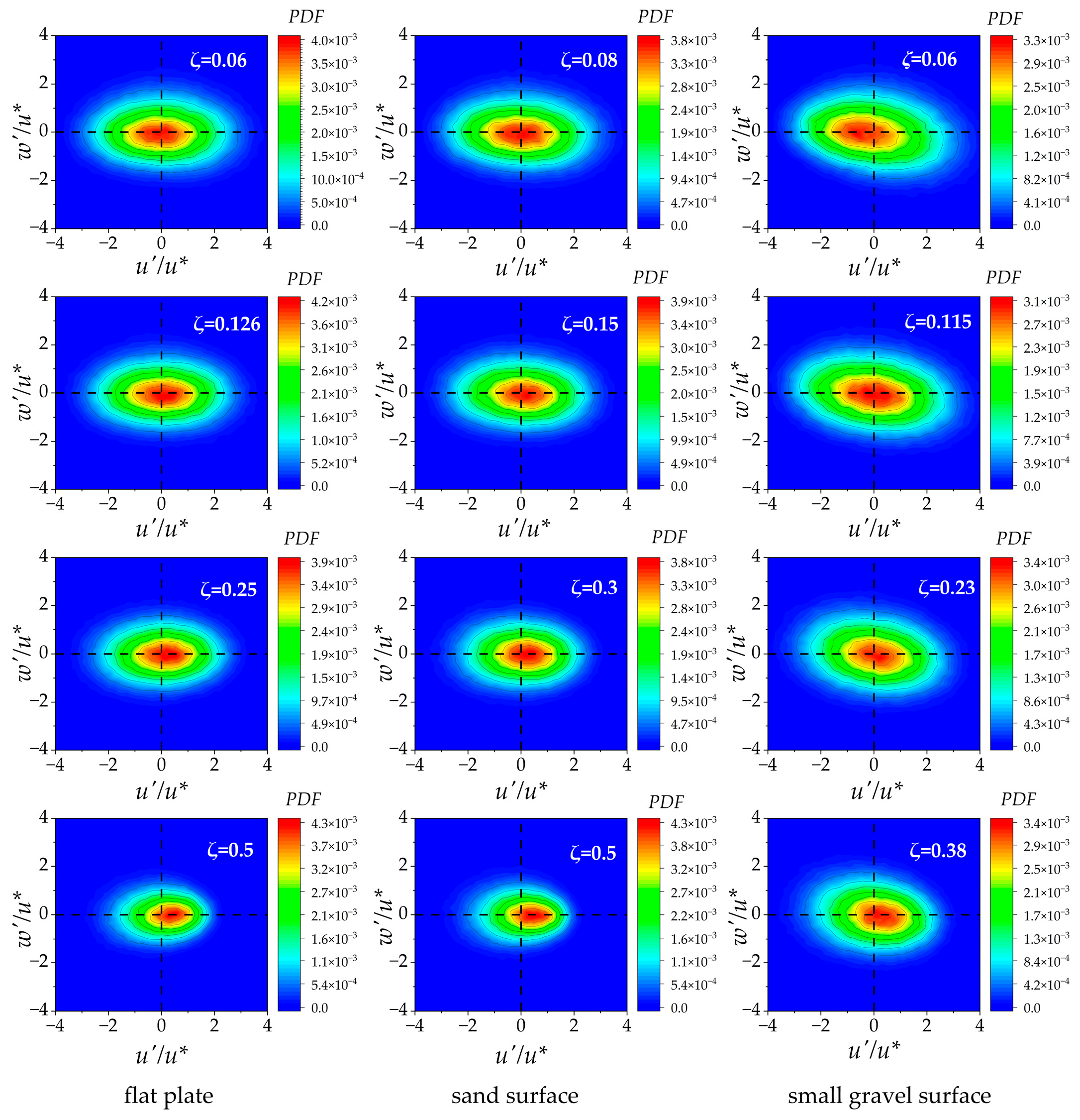
Given that velocity fluctuations in the near-wall region exhibit distinct variation patterns influenced by surface roughness elements, this study focuses on analyzing the probability density distributions of the normalized velocity fluctuations for a Reynolds number of 4.93 × 10⁵ and at normalized heights ζ < 0.5 across all surfaces. To analyze the turbulent structure of the wind velocity fluctuations, the quadrant analysis method was employed [28]. This technique categorizes the instantaneous fluctuating velocities u′ and v′ into four quadrants based on their signs:

Q1 (u′ > 0, v′ > 0): Outward Interaction, characterized by high-speed fluid moving upward.

Q2 (u′ < 0, v′ > 0): Ejection, characterized by low-speed fluid moving upward.

Q3 (u′ < 0, v′ < 0): Inward Interaction, characterized by low-speed fluid moving downward.

Q4 (u′ > 0, v′ < 0): Sweep, characterized by high-speed fluid moving downward.

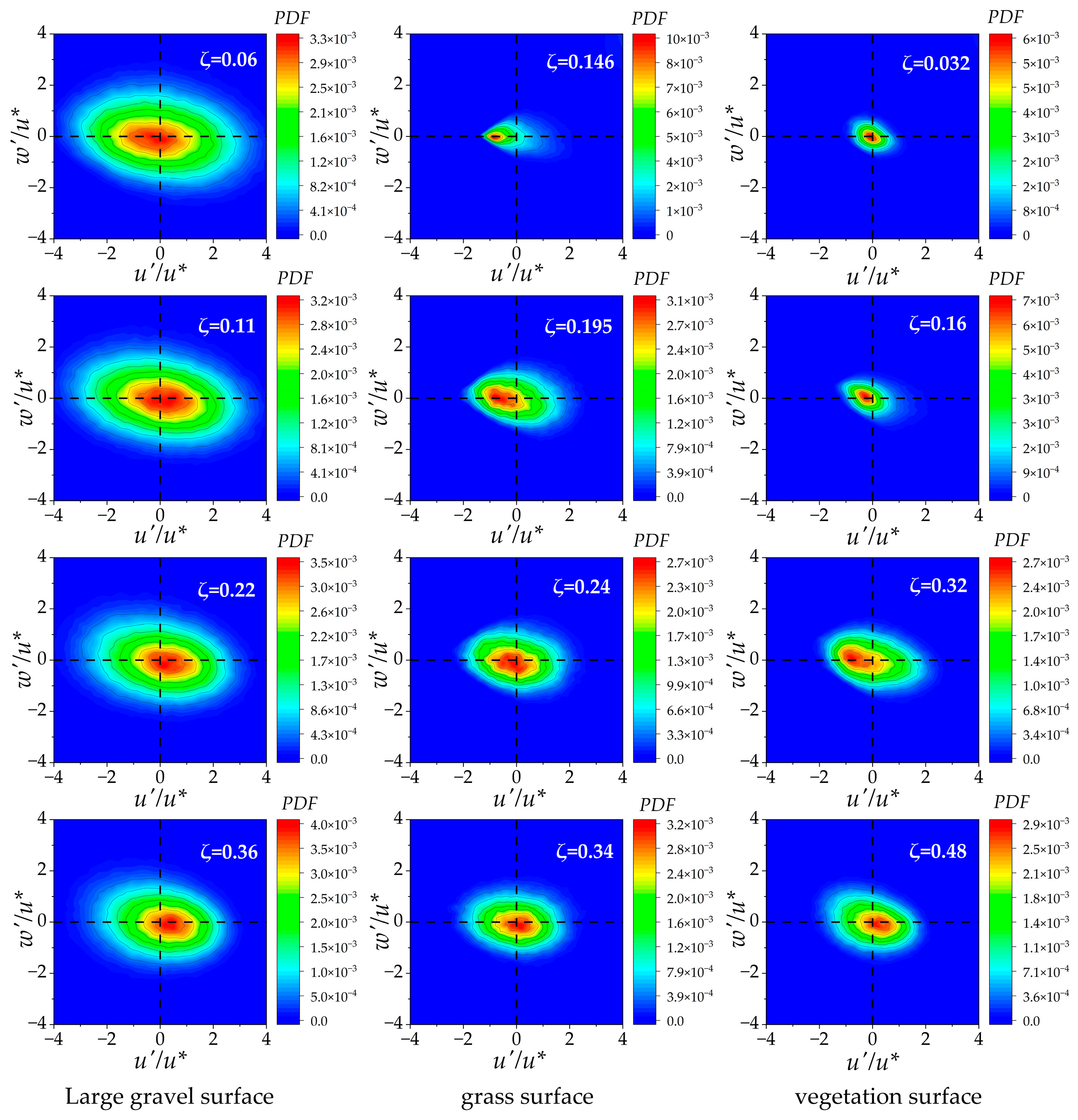
Among these, turbulent events in the Q2 and Q4 quadrants contribute most significantly to the momentum flux and constitute the primary source of Reynolds stress. Figure 5 and Figure 6 present probability density distribution contours using u*-normalized fluctuating velocities. Using u* for dimensionless normalization does not affect the distribution across the four quadrants.

Figure 5 and Figure 6 present the quadrant distributions of velocity fluctuations at various heights for all surfaces at Re = 4.93 × 10⁵. The flat plate and sand surface exhibit similar trends in quadrant distribution with the increasing height, with four quadrants maintaining a relatively balanced contribution. Near the surface, the probabilities of turbulent events across quadrants are comparable. As the height increases, the velocity fluctuations gradually become more concentrated in the Q1 and Q4 quadrants. The small and large gravel surfaces share essentially identical quadrant distribution patterns. Near the surface, Q2 occurs with significantly higher probability than in other quadrants, indicating the dominance of ejections. With the increasing height, the probability of Q2 decreases progressively, while the probability of Q4 increases, ultimately leading to the dominance of high-speed downward sweeps. The grass surface exhibits a distribution pattern in the canopy-top region (ζ = 0.147) distinct from the gravel surfaces. Immediately adjacent to the canopy, the normalized velocity fluctuations are relatively low and are predominantly concentrated in the Q2 and Q3 quadrants, forming a sharp probability peak. This peak decays rapidly with increasing height. The turbulence structure shifts initially toward the Q2 quadrant and then transitions toward the Q1 and Q4 quadrants, ultimately becoming concentrated in the Q4 quadrant. The quadrant distributions across heights for the vegetation surface differ markedly from those of the other surfaces. At all heights, the fluctuations show a concentrated distribution along the diagonal (Q2–Q4) direction, implying that the momentum transport is primarily contributed by Q2 and Q4. Similar diagonal-oriented distributions have been reported in canopy turbulence studies and are recognized as a structural feature resulting from the strong shear layer formed at the canopy top [29]. As the height increases from within the canopy upward, the distribution of velocity fluctuations over the vegetation surface initially shifts overall towards the Q2 quadrant, and then progressively transitions toward the Q4 quadrant.

With the exception of the vegetation surface, the intensity of velocity fluctuations diminishes progressively with height for all other surfaces, and the region of the maximum probability density in the distributions gradually shifts from the vicinity of u′ < 0, v′ ≈ 0 toward u′ > 0, v′ ≈ 0. In contrast, the vegetation surface exhibits a different behavior: its fluctuation intensity initially increases and then decreases with height. Near the surface, the PDF peak is located around u′ ≈ 0, v′ ≈ 0. As the height rises, this peak initially shifts toward the Q2 quadrant (u′ < 0, v′ > 0) at intermediate heights, and then further transitions to the Q4 quadrant (u′ > 0, v′ < 0) near the canopy top. Based on the quadrant distribution characteristics described above, it is evident that the flat plate and sand surface follow similar patterns; the two gravel surfaces share comparable behaviors; the grass and vegetation surfaces exhibit distinct distribution patterns. Therefore, the subsequent analysis will focus on a comparative investigation of four representative surfaces: the flat plate, small gravel, grass, and vegetation surface. 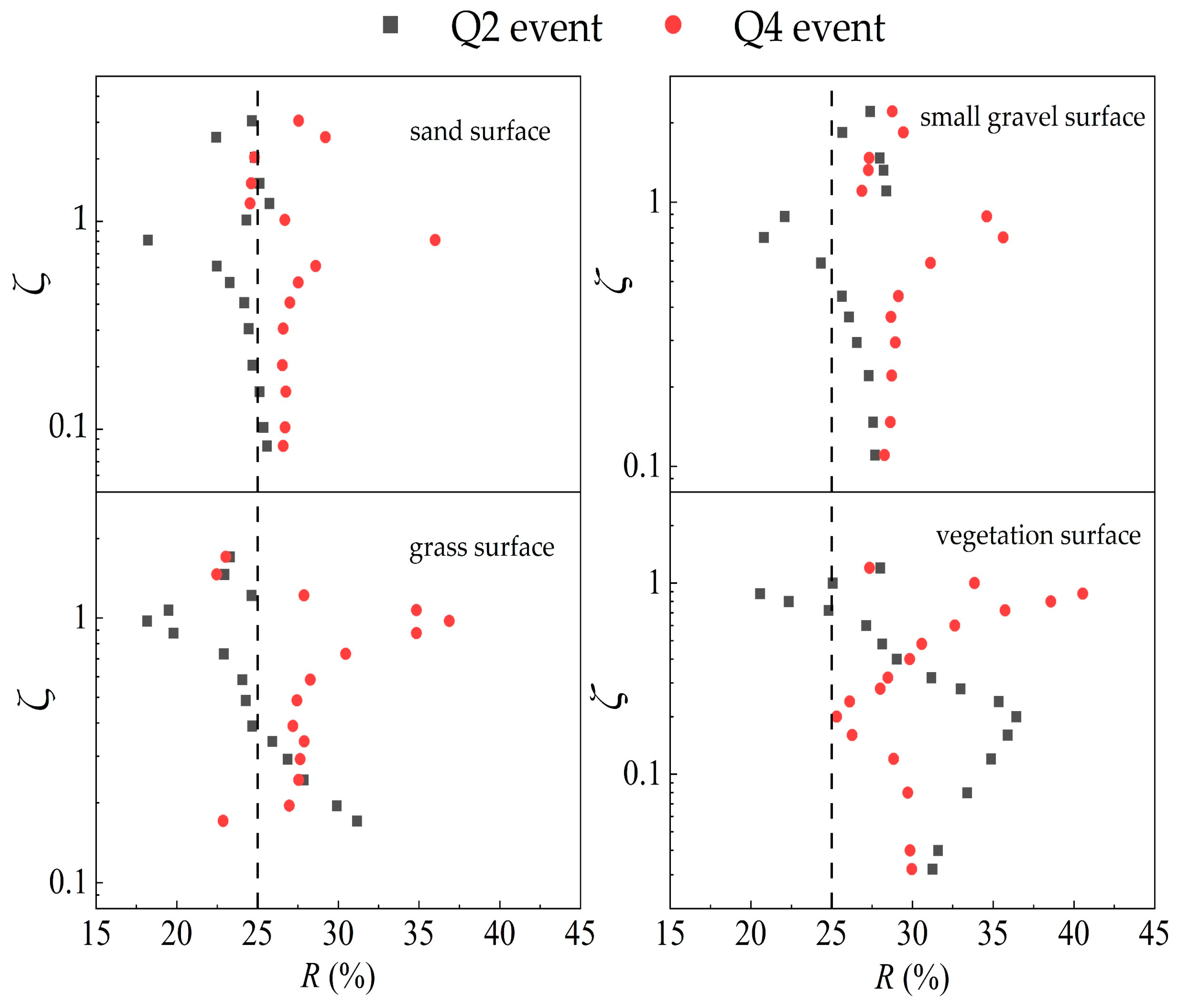Figure 7 illustrates the variation in the fractional contributions of Q2 and Q4 with the height for these four surfaces, while Figure 8 presents the combined contribution of Q2 and Q4 as a function of height.

As shown in Figure 7 and Figure 8, the probability distributions of turbulent quadrants exhibit significant differences and inherent patterns with non-dimensional height across different surfaces. Both the sand and small gravel surfaces are dominated by Q2 and Q4 in the near-surface layer, with each contributing over 25%, reflecting the typical structure of a shear-driven boundary layer. For ζ < 0.2, the probabilities of Q2 and Q4 events remain nearly constant with increasing height. However, their contributions demonstrate opposite trends at greater heights. The probability of Q2 events gradually decreases, while that of Q4 events steadily increases. Near the top of the boundary layer, the growth in Q4 accelerates, indicating enhanced downward momentum transport by large-scale turbulent structures.

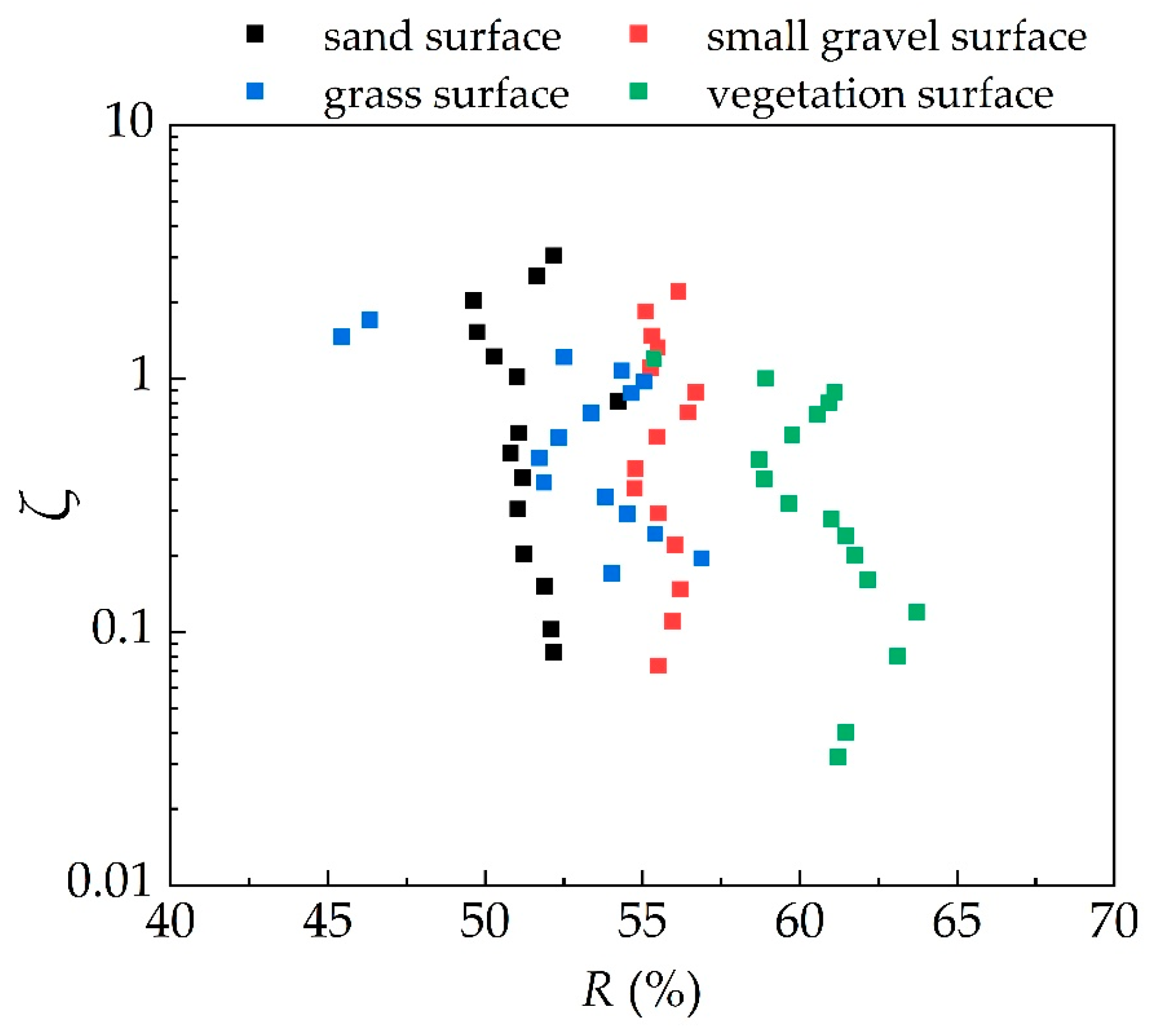
For all surfaces, the combined contribution of Q2 and Q4 gradually increases with the height from ζ ≈ 0.45 to ζ ≈ 1. When ζ < 0.55, the sand surface shows only a slight decrease in the combined contribution with the height, further confirming its relatively simple turbulence structure dominated by wall shear. In contrast, the small gravel surface exhibits a distinct peak near ζ ≈ 0.15, indicating that the roughness elements enhance the synergistic effect between Q2 and Q4 at this height, forming a zone of maximum momentum transport.

The grass surface exhibits distinct behavior in the canopy-top region (ζ = 0.147), where the probability of Q4 events is 23%, significantly lower than the 31% probability of Q2 events. As height increases, the probability of Q4 events rises markedly, while that of Q2 events decreases substantially. The two probabilities become equal near ζ = 0.24, and beyond this height the trends in Q2 and Q4 probabilities gradually converge toward those observed for the sand and small gravel surfaces. The combined Q2 + Q4 contribution increases with height, reaching a peak near ζ = 0.2, and then declines noticeably over the range ζ = 0.2–0.5.

The quadrant distribution of the vegetation surface differs markedly from all other surfaces. Within the canopy (ζ = 0.08–0.2), the trends of Q2 and Q4 are opposite to those described above. The probability of Q2 events increases with height, while that of Q4 gradually decreases. This is attributed to the unique modulation of the turbulent flow field by the tall, dense canopy. The dense foliage strongly blocks and filters the airflow, suppressing Q2 while enhancing Q4, leading to an inversion of the momentum flux mechanism (i.e., the local turbulent momentum flux becomes dominated by downward sweeps). As the height increases further above the canopy, the probabilities of Q2 and Q4 gradually converge toward distributions characteristic of conventional boundary layers. Regarding the combined Q2 + Q4 contribution, it increases with height from the near-surface layer, reaching a peak at the bottom of the vegetation canopy (ζ ≈ 0.1), and then decreases to a minimum near the canopy top (ζ ≈ 0.3). This trend aligns with findings from Böhm’s canopy turbulence experiments, which reported the dominance of sweep within dense vegetation [30]. Although the combined Q2 + Q4 contribution decreases slightly above the canopy, it remains at a relatively high level up to the top of the boundary layer. This indicates that the strong shear layer generated at the canopy top not only locally intensifies turbulence (e.g., via Kelvin–Helmholtz vortex shedding), but also transmits energy upward through turbulent transport, thereby profoundly influencing turbulence production and momentum flux across the entire boundary layer depth.

3.3. Turbulence Intensity and Reynolds Stress of Different Underlying Surfaces

The quadrant distributions of velocity fluctuations at various heights are closely related to Reynolds stress and turbulence intensity across all surfaces. The relative contributions of Q2 and Q4 at each height govern the variation in Reynolds stress with height. Subsequent analyses will examine the variation in Reynolds stress and streamwise turbulence intensity with height for the four selected surface types.

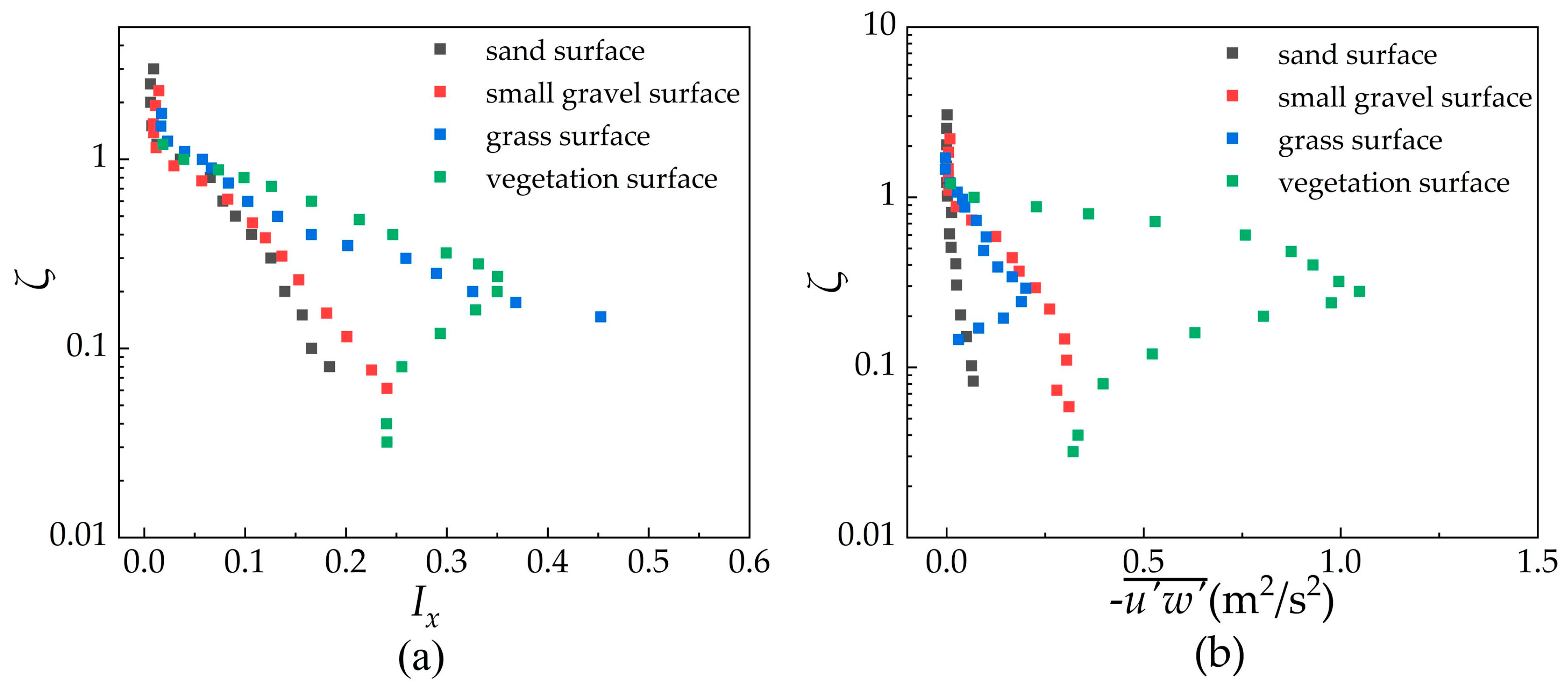
Figure 9 presents the distributions of streamwise turbulence intensity (I_x) and Reynolds stress ($-\overline{u^{\prime }{w}^{\prime }}$) with non-dimensional height for four representative surfaces at Re = 4.93 × 10⁵, i.e., flat plate, large gravel, grass, and vegetation. Streamwise turbulence intensity is a dimensionless measure of the intensity of velocity fluctuations in the streamwise (longitudinal, x-axis) direction. It quantifies the relative level of turbulence and is defined as the ratio of the root-mean-square (RMS) of the fluctuating streamwise velocity (${\mathrm{u}}_{\mathrm{rms}}^{‘}=\sqrt{\overline{{\mathrm{u}}^{‘2}}}$) to local mean streamwise velocity ($\overline{u}$), i.e., $I_x=\sqrt{\overline{{\mathrm{u}}^{‘2}}}/\overline{u}$.

Figure 9a indicates that the streamwise turbulence intensity over the vegetation surface exhibits a unimodal distribution with height, peaking near ζ ≈ 0.3 (close to the canopy top). In contrast, the turbulence intensity for the other surfaces decreases monotonically with height, approaching zero at the top of the boundary layer (ζ = 1).

Figure 9b indicates that the vertical distributions of Reynolds stress differ notably among the surfaces. Both the vegetation and grass surfaces show a unimodal pattern, increasing to a peak before gradually decreasing with height, while the sand and small gravel surfaces generally exhibit a monotonic decrease with height. For the sand and small gravel surfaces, the turbulent momentum flux is primarily generated by near-surface shear and gradually dissipates with height, consistent with the local equilibrium hypothesis for classical boundary layers. Over the grass surface, turbulence is mainly generated by shear at the canopy top. The height of the most intense momentum exchange (ζ ≈ 0.25–0.3) corresponds to the location where the contributions of Q2 and Q4 are higher (Figure 7). Except very close to the surface, the turbulence structure exhibits characteristics of a typical single shear layer. In the vegetation case, the tall, dense canopy modulates the turbulence, leading to a momentum flux inversion within the canopy. Thus, although the strong shear at the canopy top (ζ ≈ 0.3) generates large-scale eddies that maximize Reynolds stress (most efficient momentum flux), turbulent events there are dominated predominantly by Q4, causing the combined Q2 + Q4 contribution to reach a minimum. In contrast, near the canopy base (ζ ≈ 0.1), both Q2 and Q4 contribute substantially, resulting in a peak in the combined Q2 + Q4 contribution. In short, the intense turbulent mixing at the vegetation canopy top enhances momentum exchange efficiency, yet the asymmetric turbulence structure inside the canopy leads to opposite behaviors in quadrant event distributions.

A comparison of turbulence intensity and Reynolds stress reveals an inconsistency in their rankings across various surfaces: the order of peak Reynolds stress magnitude (vegetation > gravel > grass > sand) differs from that of turbulence intensity (grass > vegetation > gravel > sand). This discrepancy indicates fundamental differences in the mechanisms of turbulence energy production and dissipation among the surfaces. Although the grass surface generates the most intense velocity fluctuations (highest turbulence intensity), its flexible and dense canopy structure dissipates a substantial portion of the turbulent energy through friction with the plants. Consequently, the proportion of energy available for vertical momentum transport is relatively low, resulting in a lower peak Reynolds stress. The underlying physical mechanism is that the flexible, dense vegetation canopy dissipates substantial turbulent energy through plant sway and leaf drag, which consumes turbulent kinetic energy and reduces the efficiency of effective momentum transport. Wind tunnel studies by Finnigan and Brunet et al. demonstrated that the swaying of crops (the Honami phenomenon) can dissipate part of the turbulent energy, thereby weakening the effective transport of turbulent momentum flux [31,32]. In contrast, the tall and rigid vegetation surface (simulating shrubs or forests) organizes turbulent structures more effectively, converting turbulent energy more efficiently into vertical momentum exchange. This leads to the highest peak Reynolds stress, reflecting the greatest momentum flux efficiency and aerodynamic roughness. For low-lying rigid surfaces such as sand and gravel, turbulence originates primarily from bottom shear. As roughness decreases, both turbulence intensity and Reynolds stress diminish accordingly, following distributions consistent with classical wall-bounded turbulence theory.

Evidently, higher turbulence intensity does not directly correspond to enhanced momentum transport efficiency. The geometric and mechanical properties of the underlying surface, such as roughness element height, density, and flexibility, fundamentally determine both the distribution of turbulent energy and the characteristics of momentum exchange in the boundary layer by modulating the turbulence structure. This finding aligns with the existing literature, which demonstrates that high-roughness canopies are far more effective than low-roughness surfaces at absorbing near-surface momentum and modulating turbulence [33,34]. Furthermore, the unstable shear flow at the canopy top can significantly enhance turbulent exchange efficiency [35]. Therefore, the dominant quadrant patterns for different surfaces can be summarized as follows: the grass surface is dominated by Q2; the sand and small gravel surfaces are dominated by Q4; and the vegetation canopy shows a Q2 dominance accompanied by significant Q4 near the canopy top. This variation directly influences the magnitude and distribution of Reynolds stress: Q4 dominance leads to more intense downward momentum transport concentrated near the surface, yielding higher near-wall Reynolds stress, whereas Q2 dominance results in a more gradual momentum transfer, with the stress peak shifting upward and generally having a lower magnitude.

3.4. Turbulent Production and Dissipation Rate of Different Underlying Surfaces

To further analyze the characteristics of turbulent transport within the boundary layers over multiple surfaces, it is necessary to examine the spatiotemporal patterns of TKE in terms of its production, transport, dissipation, and conversion. This involves analyzing the vertical distributions of the turbulence production term (P_k) and the dissipation rate (ε) from the TKE budget equation. The production term represents the generation of TKE by the shear of the mean flow, while the dissipation rate denotes the dissipation rate of turbulent energy. For the dissipation rate, directly measuring the instantaneous spatial velocity gradient via Equation (4) is technically extremely difficult. The Taylor frozen turbulence hypothesis can be used to simplify this calculation, ultimately reducing the formula for the dissipation rate to Equation (5).

For the calculation of turbulent kinetic energy dissipation rate ε, Taylor’s frozen turbulence hypothesis (hereafter TH) was applied to convert temporal derivatives into spatial gradients [36]. TH postulates that turbulent structures are advected past the measurement point without significant evolution, allowing the transformation ∂/∂x = (1/ū)∂/∂t. This conversion is essential for estimating the velocity gradients (∂u_i/∂x_j) required in the dissipation rate calculation. If TH is not strictly valid for these measurements, inevitable errors are introduced when estimating Lagrangian quantities [37,38]. The validity of TH requires relatively low turbulence intensity; according to the criterion proposed by Willis and Deardorff [39], TH is acceptable when I_x < 0.5. As shown in Figure 9, the turbulence intensities for all surfaces in this study satisfy this condition, justifying the application of TH. The formulas for calculating the turbulent kinetic energy production term P_k and dissipation rate ε are given below:

$$P_k=-\langle -\overline{u^{\prime }{w}^{\prime }}\rangle {\displaystyle \frac{\partial \langle \mathrm{u}\left(\mathrm{z}\right)\rangle }{\partial \mathrm{z}}}$$

(3)

$$\epsilon =\nu \langle {\displaystyle \frac{\partial {\mathrm{u}}_{\mathrm{i}}^{‘}}{\partial {\mathrm{x}}_{\mathrm{j}}}}{\displaystyle \frac{\partial {\mathrm{u}}_{\mathrm{i}}^{‘}}{\partial {\mathrm{x}}_{\mathrm{j}}}}\rangle$$

(4)

$$\epsilon \approx 15\nu {\displaystyle \frac{\langle ((\partial {\mathrm{u}}^{\prime })/\partial {\mathrm{t})}^2\rangle }{\mathrm{u}{\left(\mathrm{z}\right)}^2}}$$

(5)

The experimental parameters are defined as follows: $-\langle -\overline{u^{\prime }{w}^{\prime }}\rangle$ is the Reynolds stress tensor. ${\displaystyle \frac{\partial \langle \mathrm{u}\left(\mathrm{z}\right)\rangle }{\partial \mathrm{z}}}$ is the mean velocity gradient tensor. $\nu$ is the kinematic viscosity of the fluid, defined as $\nu =\mu /\rho$. This represents the fluid’s resistance to shearing motion and governs the rate at which turbulent kinetic energy is converted into heat at the smallest scales. $((\partial {\mathrm{u}}^{\prime })/\partial {\mathrm{t})}^2$ is the mean square of the streamwise velocity fluctuation time derivative. $\mathrm{u}\left(\mathrm{z}\right)$ is the local mean streamwise velocity at the measurement point. In boundary layer flows. ${\mathrm{u}}^{\prime }$ is the fluctuating component of the streamwise velocity.

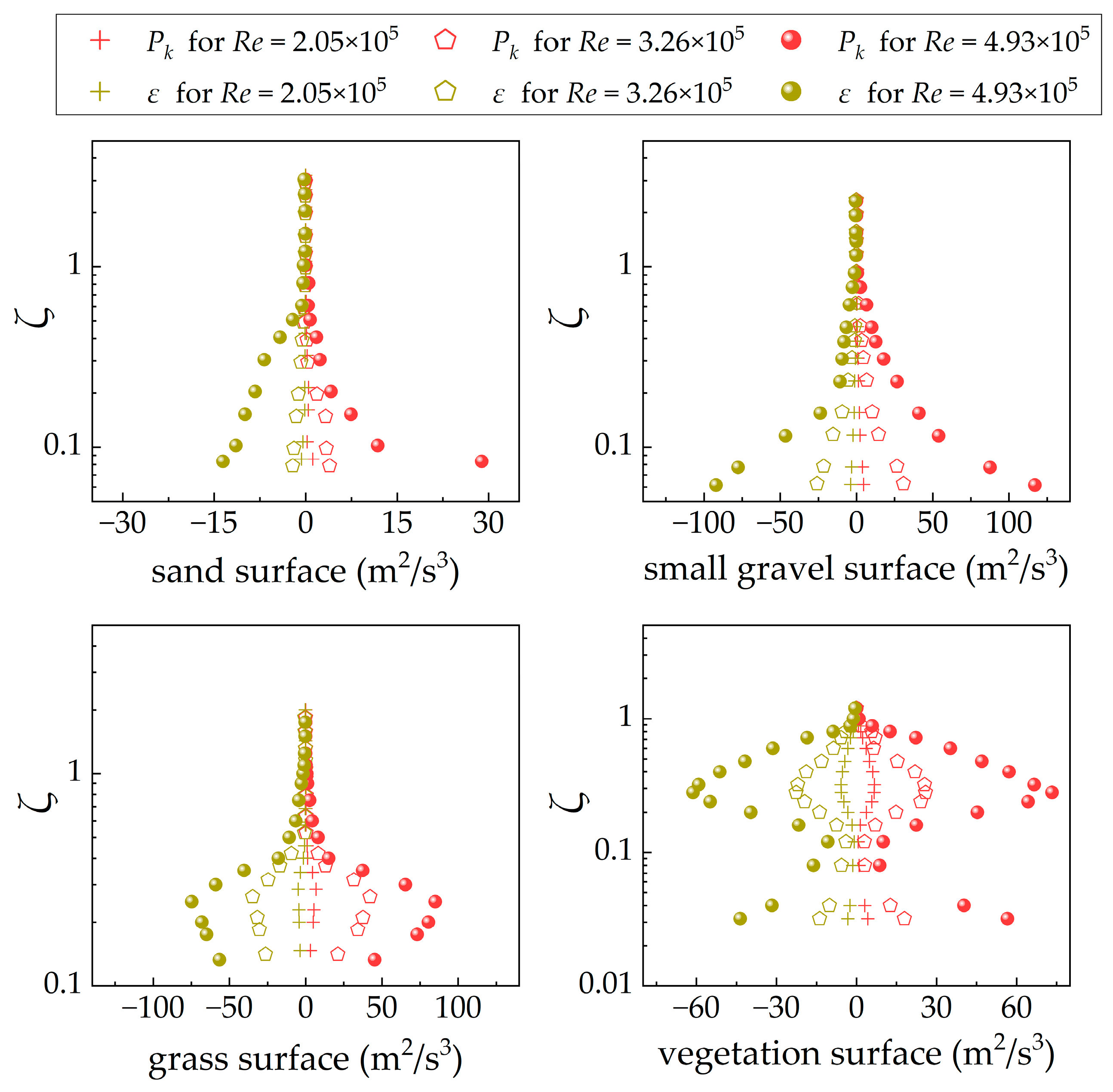
The analysis of the turbulence production and dissipation rate in the TKE budget equation for different surfaces yielded the spatial distribution patterns of TKE generation and dissipation. Figure 10 presents the distributions of the production term (red) and the dissipation rate (yellow) for four surfaces under two Reynolds numbers (Re = 2.05 × 10⁵, Re = 3.29 × 10⁵, and Re = 4.93 × 10⁵). The data points of different shapes correspond to the different Reynolds numbers.

Figure 10 presents the variation in P_k and ε with non-dimensional height for the sand, grass, small gravel, and vegetation surfaces under three Reynolds numbers. It can be observed that the response trends of P_k and ε to the changes in Re are similar across different surfaces. As Re increases, both P_k and ε at the same height increase synchronously, and this amplifying effect of higher Re becomes more pronounced closer to the surface. On smooth underlying surfaces, P_k near the ground is significantly greater than the dissipation rate. As height increases, turbulent dissipation gradually becomes dominant. For rough underlying surfaces, the pattern is similar to that of smooth surfaces, but the turbulent production term remains slightly larger than the dissipation rate with increasing height. For vegetated and grassland underlying surfaces, near the canopy layer, the turbulent production term is smaller than the turbulent dissipation rate.

For both the sand and small gravel surfaces, P_k and ε decrease monotonically with height, approaching zero near the top of the boundary layer. This reflects the trend of turbulence generated by wall shear being gradually dissipated upward. For the sand surface, the gradient of the dissipation rate ε with height remains largely unchanged across different Re values. However, its production rate P_k exhibits a steeper gradient very close to the surface at higher Re (indicating enhanced turbulence production). For the small gravel surface, both the production and dissipation rates maintain relatively high values over a certain height range near the surface. This indicates that turbulence is not merely generated and dissipated within a few millimeters of the ground, but rather is distributed more uniformly throughout a thicker roughness sublayer. The P_k and ε profiles for the small gravel surface show an inflection point near ζ ≈ 0.18—a location that corresponds to the peak Reynolds stress. For ζ < 0.18, the decline rate of both terms with height is significantly greater than for ζ > 0.18. This distribution is consistent with the local equilibrium hypothesis for classical boundary layers, where production dominates dissipation in the near-wall region, and dissipation prevails over generation farther from the wall.

For the grass surface, P_k increases significantly with height over 0.146 < ζ < 0.24, decreases markedly across 0.24 < ζ < 0.4, and then declines gradually to zero for 0.4 < ζ < 1. This vertical trend is similar to that of the Reynolds stress for the same surface, as shown in Figure 9. The dissipation rate ε follows a pattern consistent with P_k throughout the entire layer (0 < ζ < 1). These profiles further affirm that the dual-layer turbulent dynamics characteristic of flexible vegetation canopies: vortex motions near the canopy top promote reverse momentum transfer and dissipate turbulent energy, while the overlying shear layer efficiently generates TKE that sustains larger-scale motions. Notably, at canopy height (ζ = 0.146), ε exceeds P_k, indicating that canopy drag substantially alters the local turbulent energy balance.

The vegetation surface exhibits a distinct pattern in the vertical variation in P_k and ε. In the range 0 < ζ < 0.1, P_k decreases with increasing height, reaching a minimum near the canopy bottom. When 0.1 < ζ < 0.3, P_k increases rapidly, indicating that the strong shear at the canopy top drives TKE production to its peak. For 0.3 < ζ < 1, P_k then declines gently from its peak to zero. Correspondingly, the distribution of ε follows a similar trend: the dissipation rate reaches its minimum at the canopy base (ζ ≈ 0.1), peaks in the mid-upper canopy (ζ ≈ 0.3), and gradually decreases at higher altitudes, approaching P_k to achieve an energy balance.

The unimodal distribution of P_k within and above the vegetation canopy aligns with the unimodal structure of the Reynolds stress, which also peaks at the canopy top (Figure 9). This confirms that the turbulent energy is primarily generated at the canopy top and subsequently diffuses both upward and downward. This phenomenon originates from the pronounced inflection point in the velocity profile at the canopy top, which triggers instability akin to that in a free shear layer (e.g., Kelvin–Helmholtz instability), thereby generating vortex structures spanning the canopy top. These vortices are responsible for the peak in turbulence production near the canopy top. Simultaneously, they sweep high-momentum fluid into the canopy and eject low-momentum fluid out of it, resulting in the dominance of Q4 and suppression of Q2 within the canopy, as noted in the previous quadrant analysis. Research by Finnigan indicates that large-scale turbulent eddies above the canopy interact with the canopy shear layer, jointly influencing the turbulent structure within the canopy strata [40]. This explains the observed pattern that, although the P_k for the vegetation surface peaks at the canopy top, significant turbulence intensity and energy transport efficiency are maintained within a certain height range above it.

Compared with the grass surface, the vegetation surface features tall and rigid roughness elements, enabling it to generate more organized turbulent structures and convert turbulent energy more efficiently into vertical momentum flux [41]. Consequently, both the production and dissipation rates are markedly higher throughout the boundary layer for the vegetated canopy compared to the low-roughness surfaces, demonstrating pronounced non-equilibrium characteristics (P_k ≠ ε) around the canopy height. Overall, the characteristics of the turbulent energy balance for different surfaces illustrate how the height, density, and flexibility of surface roughness elements modulate the processes of turbulence production and dissipation.

3.5. Turbulent Diffusion Coefficients of Different Underlying Surfaces

The differences in turbulent characteristics across various surfaces arise from surface-morphology-induced modifications to coherent turbulent vortex structures and the associated transport mechanisms. Roughness and vegetation primarily influence turbulence by modifying near-wall shear stress distributions, inducing coherent vortices, and altering dissipation mechanisms. These factors also govern the distribution patterns of turbulent diffusion coefficients within the boundary layer over various surfaces.

Taylor’s statistical diffusion theory [42] provides the theoretical foundation for estimating turbulent diffusion coefficients, which were calculated from high-frequency streamwise and vertical velocity data measured by a two-dimensional hot-wire anemometer in a wind tunnel over various underlying surfaces at different Reynolds numbers. Accordingly, we computed $K_i^f$ via Equation (6), which expresses the diffusivity as the product of the velocity variance $\overline{v_i^2}$ and the Lagrangian integral time scale $T_{\mathit{Lfi}}$. Since Lagrangian quantities are difficult to measure directly, $T_{\mathit{Lfi}}$ was inferred from Eulerian measurements using the formula shown in Equation (7), where $T_{\mathit{Efi}}$ is the Eulerian integral time scale and β is the ratio between Lagrangian and Eulerian time scales. Following Hanna [43], β was estimated using the empirical formula β = 0.7/$I_i$. With the Eulerian integral time scale, the characteristic relaxation time is obtained by integrating the autocorrelation coefficient $R_{\mathit{Ei}}\left(\tau \right)$ of the fluctuating velocity in the i-direction over the time scale, where the upper integration limit $\tau$ is the first zero-crossing point of $R_{\mathit{Ei}}$. Taylor’s frozen hypothesis (TH) was invoked to ensure the validity of this approach, as its applicability was verified as described in Section 3.4. The calculation formula is given below.

$$K_i^f=\overline{v_i^2}{T}_{\mathit{Lfi}}$$

(6)

$$T_{\mathit{Lfi}}{=\beta T}_{\mathit{Efi}}$$

(7)

$$T_{\mathit{Efi}}={{\displaystyle \int }}_0^{\mathrm{\tau }}{R}_{\mathit{Ei}}\left(\tau \right)d\tau$$

(8)

$$R_{\mathit{Ei}}\left(\tau \right)={\displaystyle \frac{u_i\left(t+\tau \right)·u_i\left(\mathrm{t}\right)}{{\sigma }_i^2}}$$

(9)

where $K_i^f$ represents the turbulent diffusion coefficient of fluid, in which the subscript i denotes the streamwise direction or vertical direction. v_i is the RMS value of the fluid velocity fluctuations. $I_i$ is the turbulent intensity of the streamwise direction or vertical direction. $T_{\mathit{Lfi}}$ is the Lagrangian characteristic relaxation time of fluid, $T_{\mathit{Efi}}$ is the Eulerian characteristic relaxation time of fluid, and $R_{\mathit{Ei}}\left(\tau \right)$ is the Eulerian velocity autocorrelation coefficient.

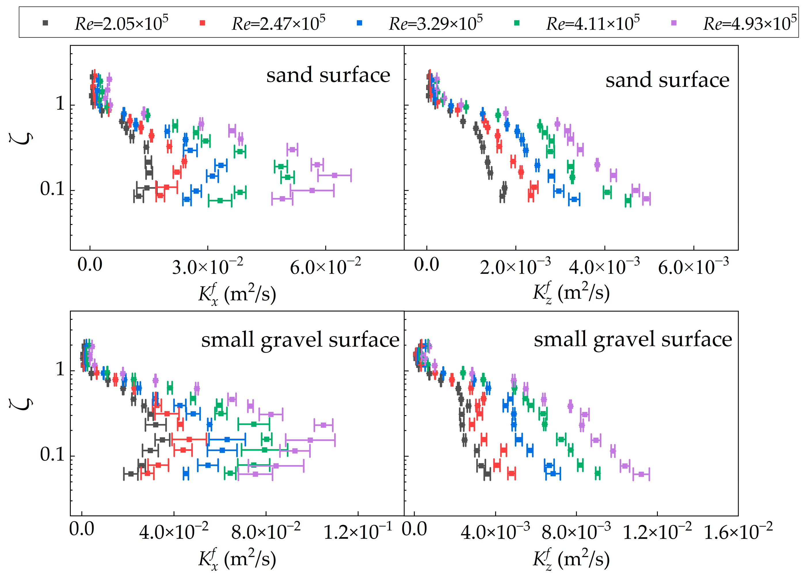
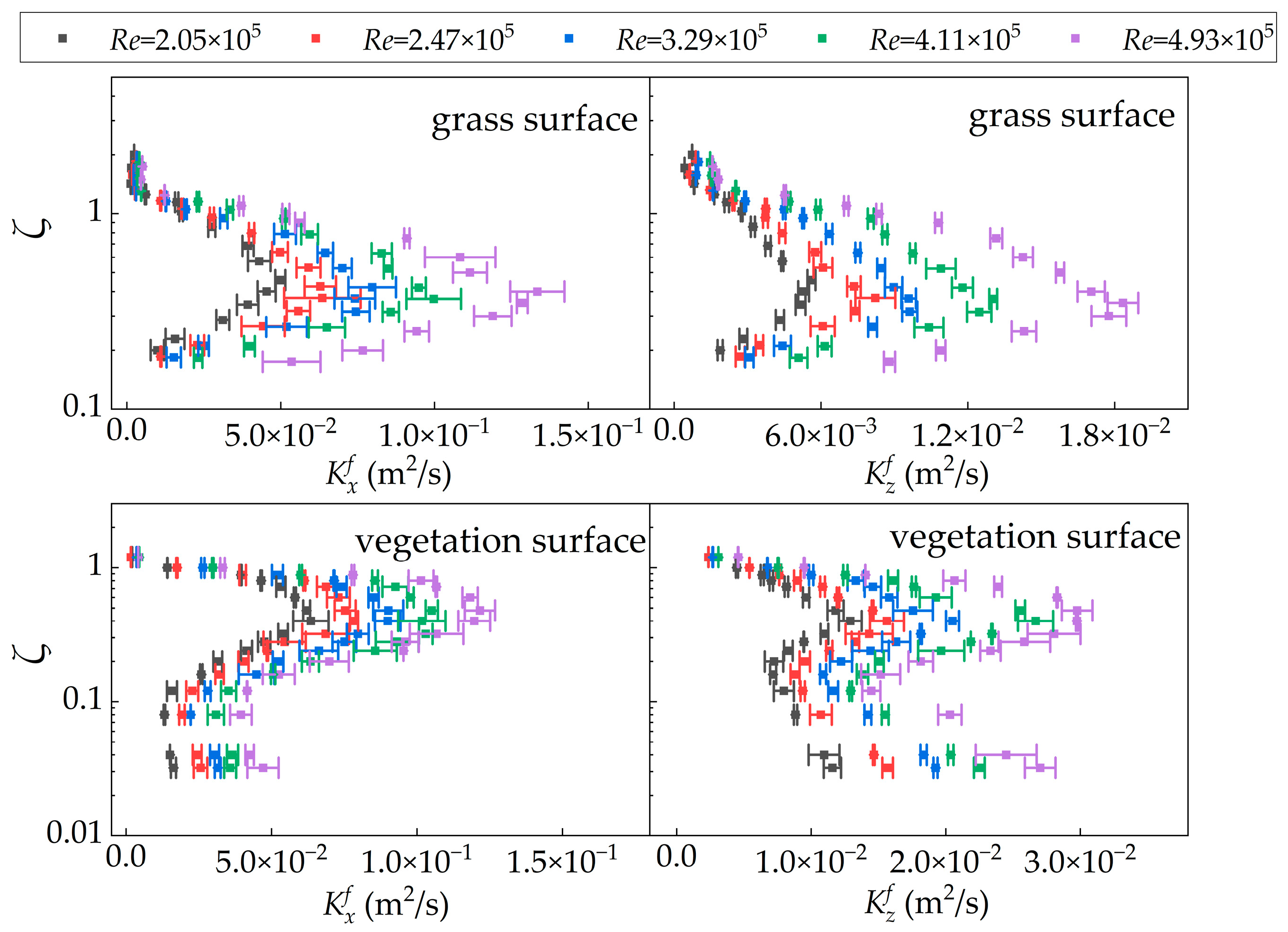
Figure 11 and Figure 12 present the vertical distributions of the streamwise (K_x) and vertical (K_z) turbulent diffusion coefficients for the different surfaces. It can be observed that higher Reynolds numbers correspond to larger K_x and K_z values at the same height, indicating that enhanced turbulence intensity improves turbulent diffusion capacity. For both the sand and small gravel surfaces, K_x exhibits a unimodal distribution with height. The height of its peak decreases from approximately ζ = 0.2 to ζ = 0.15 as Re increases from 2.05 × 10⁵ to 4.93 × 10⁵. Their K_z decreases with height, with the sand surface showing a change in the decay rate near ζ ≈ 0.6, while the rate of decrease for ζ > 0.6 is greater than for ζ < 0.6.

The grass surface shows unimodal distributions for both K_x and K_z, with peaks occurring roughly at ζ ≈ 0.45 and ζ ≈ 0.4, respectively (shifting slightly downward with increasing Re). The distributions of K_x and K_z of the vegetation surface are the most complex. K_x shows a slight decreasing trend in the immediate vicinity of the surface (ζ ≈ 0.03–0.1), and then increases rapidly with height to reach a peak near ζ ≈ 0.5. With a further increase in height, K_x decreases rapidly to zero. K_z follows a similar pattern to K_x, but with a local peak at ζ ≈ 0.03, where K_z diminishes more markedly compared to K_x within the range ζ ≈ 0.03–0.1. More specifically, K_z decreases significantly within 0.03 < ζ < 0.15, and subsequently increases again in the layer 0.15 < ζ < 0.4, culminating in the main peak at ζ ≈ 0.4. For ζ > 0.4, K_z declines rapidly from this peak to zero with further increment in height.

4. Discussion

Integrating the results on quadrant contributions, Reynolds stress, and energy balance reveals that the turbulent diffusion characteristics of each surface are closely associated with their turbulent structures. For sand and gravel surfaces, previous research confirms our observation that turbulence is mainly generated by bottom shear [44], where the streamwise diffusion coefficient K_x peaks near the surface (ζ ≈ 0.2) and then decays continuously with height, mirroring the distribution trend of the combined Q2 + Q4 contribution. Meanwhile, the vertical diffusion coefficient K_z decreases throughout the boundary layer with increasing height, consistent with the behavior of Reynolds stress, which also reaches its maximum in the near-surface layer before decaying monotonically; these results are consistent with the observations of Song, S. [45].

For the grass surface, the turbulent diffusion coefficients reach their peak near the canopy top (ζ ≈ 0.4–0.45), corresponding to the concurrent maxima in both the TKE production term and the Reynolds stress at this height. Above this level, the diffusion capacity declines rapidly as the dissipation of turbulent energy becomes dominant—an interpretation supported by the study conducted by Dwyer, M.J. [46]. The relationship among the turbulent parameters reflects the dual influence of the grass canopy on the flow. On one hand, the strong shear instability at the canopy top generates large-scale vortex structures that greatly enhance local turbulent mixing efficiency. On the other hand, the canopy’s blocking effect restricts both the downward penetration of turbulence and the upward transfer of energy, resulting in a distinct turbulent pattern within the canopy. Although the grass surface exhibits the highest turbulence intensity in the near-surface layer (Figure 9a), its flexible, dense canopy dissipates a substantial portion of the turbulent energy, with ε significantly exceeding P_k. Consequently, not all of the shear from the mean flow is converted into vertical transport, causing the Reynolds stress to approach zero very close to the ground as turbulent energy is locally absorbed by the canopy. This limits the momentum flux contribution and results in near-surface turbulent diffusion coefficients approaching zero. As shown in Figure 8, the combined Q2 + Q4 contribution for the grass surface peaks at ζ ≈ 0.25. At this same height, the turbulence production term P_k also reaches its maximum, indicating the most intense turbulent momentum exchange. The joint action of Q2 and Q4 events remains dominant for ζ < 0.35, driving the momentum flux to its peak at ζ ≈ 0.35, where both the Reynolds stress and the turbulent diffusion coefficients are maximized. At greater heights, the lack of new turbulent energy sources and the dominance of dissipation cause both turbulence intensity and Reynolds stress to decay, leading to a rapid decline in turbulent diffusion capacity [47].

Therefore, the peak height of the diffusion coefficients for the grass surface reflects the combined effect of the intense shear layer at the canopy top, which generates turbulence characterized by both high fluctuation intensity and efficient momentum exchange, resulting in the strongest diffusion capacity [48]. Below this height, the energy-dissipating effect of the canopy dominates, while above it, turbulence gradually decays; both effects lead to a reduction in the diffusion coefficient. The quadrant structure for the vegetation surface is particularly distinct. The wind speed profile at the canopy top features an inflection point similar to that in a mixing layer [49], where strong wind shear gives rise to Kelvin–Helmholtz-type instability. This instability triggers and organizes the formation of periodic, paired coherent vortex structures (often referred to as “hairpin vortices” or “ordered vortices”), which generate intense, intermittent turbulent exchange at the canopy top. These vortices contain sweep-dominated cores that govern turbulent transport within the canopy. The results also indicate that the sweep events contribute predominantly to the momentum flux within the vegetation canopy. This aligns with the experimental findings of Chagot [50], who further noted that ejection events seem to have a major impact on the flow above the canopy, whereas sweep events act as a turbulence source within the canopy. The researcher emphasized that the low-speed vortices (Q2) ejected upward from the canopy top play a crucial role in expelling turbulent energy from the canopy.

The bimodal structure of K_z for the vegetation surface further supports this two-layer transport mechanism; this conclusion is further corroborated by the work of Huai, W. [51]. The weak mixing in the near-surface region at the canopy bottom (the secondary K_z peak at ζ ≈ 0.03) and strong mixing at the canopy top (the primary K_z peak at ζ ≈ 0.4) work in concert to enhance the transport of momentum and scalars to greater heights. Additionally, the slight decrease in K_x in the lower part of the vegetation canopy reflects hindered momentum exchange within the canopy, while its rapid increase in the upper canopy corresponds to the highly efficient exchange generated by intense shear. In summary, the distribution patterns of the turbulent diffusion coefficients across the various surfaces reflect underlying differences in their turbulence structures. The low-lying rigid surfaces exhibit a typical single-layer shear-driven turbulence structure, whereas surfaces with flexible canopies demonstrate diffusion characteristics jointly determined by the dual-layer turbulence inside and above the canopy.

5. Conclusions

The comparative analysis of turbulence measurements over six surfaces—flat plate, sand, small gravel, large gravel, grass, and vegetation surfaces—demonstrates that the surface properties exert profound influence on turbulent structure and diffusion capacity. The main conclusions are as follows.

• Turbulence over sand and gravel surfaces is dominated by Q2 events, whereas Q4 events prevail near the surface over vegetation and grass surfaces. This shift in quadrant dominance accounts for the observed differences in momentum flux. Q4 events enhance near-surface transport by carrying high-speed fluid downward, while within canopies, large-scale Q4 structures act as the primary turbulence source, yielding sweep-dominated fluxes. Above the canopy, Q2 events play a key role in ejecting low-speed fluid and promoting exchange in the overlying flow. Thus, surface turbulence can be interpreted as a blend of Q4 and Q2 dominance, which directly modulates momentum transport efficiency.
• Reynolds stress and TKE production are markedly higher over rough and vegetation surfaces than over smooth ones, though their increases are not proportional. Rough and canopy surfaces often achieve greater mixing efficiency without a commensurate rise in TKE production, as seen for the grass canopy, where production can even decline. This suggests that vegetation and roughness elements enhance turbulent transport through organized coherent structures rather than solely through local shear. A portion of the shear energy is dissipated directly by drag rather than contributing to increased Reynolds stress.
• The balance between turbulent energy production and dissipation varies with surface type. While smooth surfaces approach a state of local equilibrium (production ≈ dissipation), rough and canopy surfaces demonstrate strong non-equilibrium. This imbalance indicates that turbulent diffusion here is driven more by transient large eddies than by steady gradient transport—a key consideration for improving canopy turbulence models. Canopies introduce instability modes such as mixing-layer vortices, which boost mixing efficiency without necessarily increasing TKE production proportionally.
• Turbulent diffusion coefficients elevate significantly with surface roughness and canopy height, and their vertical distributions change accordingly. For sand and small gravel surfaces, the streamwise diffusion coefficient exhibits a single narrow peak of modest magnitude, while the vertical coefficient decays monotonically with height. For both grass and vegetation surfaces, the distribution patterns of their streamwise and vertical turbulent diffusion coefficients are similar. The vertical diffusion coefficient is larger for vegetation surface. The vegetation canopy extends the turbulent mixing length in the lower atmosphere and introduces canopy-scale large eddies.
• The turbulent diffusion coefficients derived in this study reveal surface-dependent dispersion mechanisms with direct implications for pollutant transport. Over rigid surfaces (sand, gravel), maximum diffusion occurs near the surface and decays with height, confining pollutants to the lower boundary layer. Over flexible canopies (grass, vegetation), a two-layer regime emerges: weak mixing within the canopy limits near-ground dispersion, while intense shear at the canopy top generates coherent vortices that efficiently vent pollutants upward. This explains how vegetation canopies can simultaneously trap pollutants near the surface and facilitate their rapid export to higher altitudes—a dual role critical for understanding urban air quality and surface–atmosphere exchange. These findings underscore the need for surface-specific parameterizations in pollutant dispersion models. For example, Eulerian models (WRF-Chem, CMAQ) should implement two-layer K-theory and use measured TKE production/dissipation rates to refine closures. CFD simulations can leverage observed Reynolds stresses and quadrant contributions to validate sub-grid-scale models.

In summary, turbulence across various surfaces can be understood as a continuum between two fundamental mechanisms: classical wall turbulence (characterized by ejection events and boundary-layer structures) and free shear turbulence (dominated by sweep events and large eddies). The smooth flat plate leans toward the former, the vegetation canopy toward the latter, and rough gravel surfaces lie in between, though closer to the latter. This conceptual framework offers a constructive basis for understanding and predicting turbulent diffusion coefficients under diverse surface conditions.