CSCGAN: Cross-Space Contrastive Learning for Blind Image Inpainting

Abstract

Existing general image inpainting works require the user to customize a mask to indicate the region to be inpainted. However, the mask is often hard to calibrate accurately in real-world applications, e.g., graffiti removal. Blind image inpainting aims to automatically restore the degraded image into the visually reasonable one without a priori mask to indicate the area to be repaired. So far, most proposed blind inpainting methods convert the task into general inpainting by predicting the mask before inpainting. However, these methods are highly dependent on mask prediction results, which may produce inferior inpainting results if the prediction is inaccurate. To address this issue, we propose a two-stage blind inpainting framework with two novel designs: (1) cross-space contrastive learning, to remove the noise in the degraded images and realize the automatic inpainting in the latent space by reducing the distance of the degraded images and the corresponding complete images in the latent space; and (2) mask-aware adversarial training, to minimize the mutual information between the inpainted feature and the noise. Extensive experiments prove that our blind inpainting framework performs better on multiple datasets than the state-of-the-art methods.

1. Introduction

Image inpainting aims to generate semantically correct and visually plausible results on the area masked by a binary image. It allows users to remove stained areas or unwanted objects in images. Most existing general inpainting works [1,2,3,4,5,6] take a degraded image and a mask image as the input, where the mask specifies the regions in the corrupted image to be inpainted. However, manually locating degraded regions can be challenging in real-world applications, e.g., removing graffiti on artwork, correcting local color shift in photograph, or text removal.

To overcome the above problem, Ref. [7] first proposed blind image inpainting, which used only degraded images without an additional mask when repairing the degraded areas. Early works [7,8,9] focused on the repairing of fixed pattern noise, such as specific color or Gaussian noise. However, Ref. [10] pointed out that previous works were prone to distinguishing the mask area based on the fixed or predefined noise pattern rather than the harmony of context. To address this issue, they proposed using the content of other natural images with blurred edges as the noise to be removed. To remove noise that is difficult to calibrate, previous work [8,9,10] used an intuitive approach, which transforms the task into the general inpainting task by introducing a mask prediction module before inpainting. But they ignored the essential difference between blind inpainting and general inpainting. Considering that the noise comes from natural images, the semantic distributions of the valid and the noise regions are the same. It may be extremely difficult to predict the noise region in the degraded images accurately. Therefore, the subsequent inpainting based on the predicted mask may suffer from the incorrect prediction, which will lead to inferior results with severe artifacts.

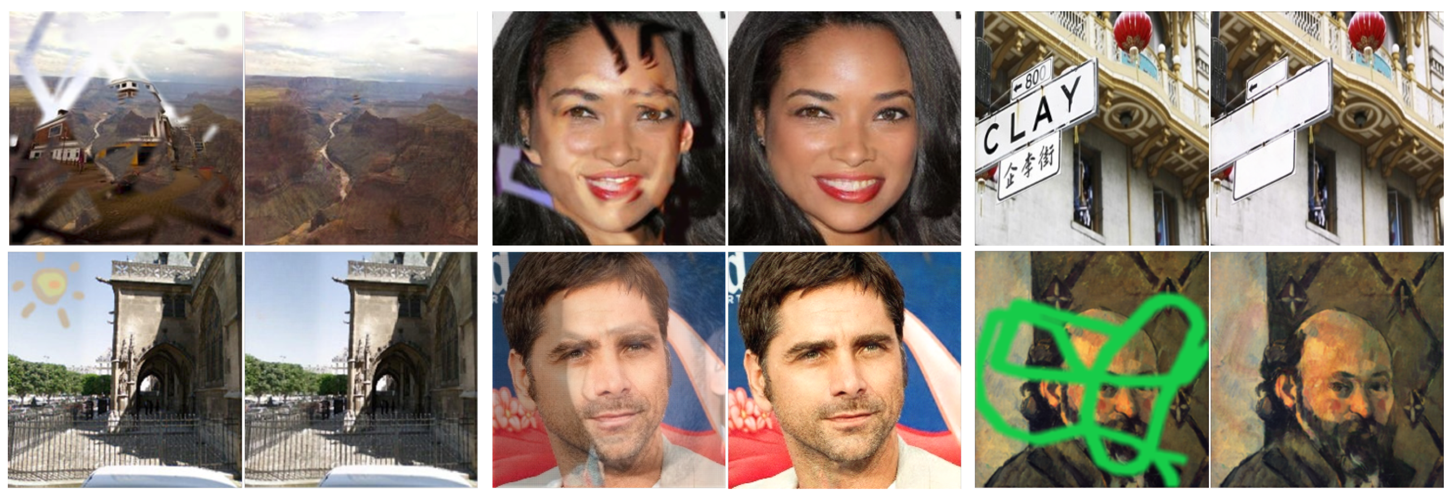
To address this issue, inspired by existing contrastive learning studies [11,12], we propose a mask-prediction-free blind inpainting framework, which achieves blind inpainting of the degraded images in the latent space through two novel constraints named cross-space contrastive loss and mask-aware adversarial loss. Some blind repair results are presented in Figure 1. Concretely, we first define the set composed of all ground-truth images as the complete image space and all noise-polluted images as the degraded image space. Then, cross-space contrastive learning is utilized to realize the automatic inpainting by reducing the distance of the degraded images and the corresponding complete images in the latent space. That is to say, cross-space contrastive learning uses latent space as a bridge to connect the degraded image space and the complete image space. This is accomplished by our proposed cross-space contrastive (CSC) loss. To avoid mapping deviation caused by the CSC loss, we introduce mask-aware adversarial (MAA) training that plays an adversarial game between the encoder and the mask-aware discriminator to minimize the correlation between the noises and the inpainting results. To ease the training pressure on limited computing resources, we couple the above design in a two-stage framework consisting of an inpainting network and a refine network.

We summarize the contributions of our work as follows:

• A mask-prediction-free framework is proposed for blind inpainting. Our method does not need to predict the noise area, thus avoiding inferior inpainting results caused by inaccurate mask prediction.
• Two novel constraints named cross-space contrastive loss and mask-aware adversarial loss are proposed for blind inpainting. To the best of our knowledge, we are the first to introduce contrastive learning to blind inpainting task.
• We propose the first blind inpainting metric called GCM, which can reasonably measure the quality of blind inpainting.
• Extensive experiments on benchmark datasets prove that our method achieves better quality than the state-of-the-art methods.

2. Related Work

2.1. Image Inpainting

Image inpainting is a classic ill-posed computer vision problem. Here, we focus on deep-learning-based methods. Some methods [13] took the lead in proposing an encoder–decoder structure inpainting network, which proved that deep learning methods are useful in the field of image inpainting. Most subsequent researchers split the inpainting task into similar coarse-to-fine subtasks to improve performance. The constraints of the coarse stage can be low-resolution patches or some other low-level features, such as edge maps [4], gradient maps [14], grayscale graphs [15], etc. Other studies like [6] proposed that the corrupted image can be mapped to the latent space. They manipulated the latent code and then translated it back to the pixel space to obtain more diverse or natural inpainting results. CMT [16] introduced a continuously masked transformer for image inpainting, highlighting the importance of mask-aware global context modeling. STNet [17] placed more emphasis on restoring structural consistency during completion. CTSTNet [18] further extended this line by jointly considering structure restoration and texture reconstruction.

2.2. Blind Image Inpainting

Unlike the general inpainting tasks, blind inpainting does not have a definite mask as a prior; so, the model is required to have the ability to determine the area to be processed. Many works, such as text removal [19], old photo restoration [20], etc., can be regarded as variants of blind image inpainting on different subtasks. The authors of [10] give the complete definition of blind inpainting for the first time. They proposed VCNet, which can be divided into a mask prediction network and an image inpainting network guided by predicted masks, realizing blind image inpainting for the first time. CAML [21] formulated blind image inpainting as a joint learning problem of mask estimation and image inpainting, and explicitly exploited their mutual contextual interactions to improve both corrupted-region localization and content completion. BIRD [22] further showed that strong generative priors can improve robustness under unknown degradations by optimizing the restored image together with the degradation parameters in a pretrained diffusion. SIME-BINet [23] enhanced blind inpainting by combining self-information modeling with prediction-mask guidance.

2.3. Contrastive Learning

Recently, contrastive learning has been used in self-supervised learning [24,25,26]. Dating back to [27], these approaches learn representations by contrasting positive pairs with negative pairs. Along these lines, Dosovitskiy [28] proposed to treat each instance as a class represented by a feature vector (in parametric form). Most of them use the noise contrastive learning evaluation method to learn an embedding where associated signals are brought together [29], in contrast with other examples in the dataset (note that similar ideas go back to classic work on metric learning with Siamese nets [30]). Inspired by the design of aligning two augmented samples in self-supervised learning, we first introduce contrastive learning into blind image inpainting tasks. MCLIR [31] exploited historical models to generate adaptive negative samples, extending contrastive learning from sample-level discrimination to model-level optimization. CPL [31] further applied contrastive learning to prompt modeling in all-in-one image restoration, where sparse prompt design and contrastive prompt regularization are used to enhance degradation discrimination and prompt-task alignment. ODCR [32] showed that contrastive regularization can also be combined with feature decoupling, where degradation-related and degradation-unrelated components are explicitly separated in an orthogonal feature space to improve restoration robustness.

3. Proposed Method

In this section, we will introduce the network structure and loss functions of our blind inpainting model.

3.1. Degraded Image Generation

The input of our blind inpainting framework is a degraded image polluted by noises. The degraded images are generated by merging the noises into the clean images, expressed as $I_{deg}=I_{noise}\odot M+I_{gt}\odot (1-M)$, where M represents a random mask blurred by a Gaussian kernel, $I_{noise}$ represents another natural image used as noise, and ⊙ represents the Hadamard product operator.

Since there are no determinate solutions for the blind inpainting task in practical applications, the desired inpainting results need to meet the following requirements: (i) be visually consistent as a whole, and (ii) faithfully retain the non-degraded areas.

3.2. Network Architecture

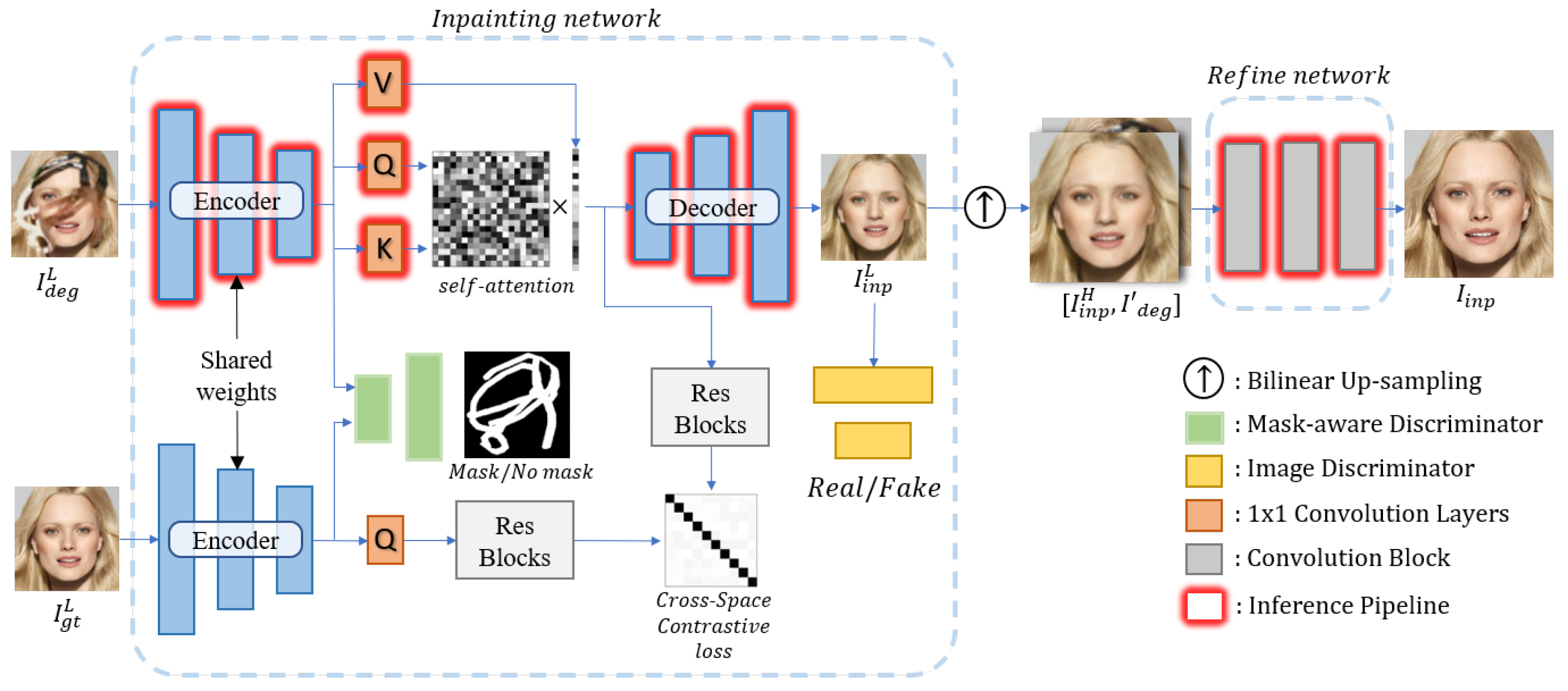
As shown in Figure 2, the inpainting stage of our network includes an encoder E, a cross-space contrastive learning module that reuses the encoder and the query layer of the self-attention module, a mask-aware discriminator $D_M$ acts on the latent space, a decoder D, and a general image discriminator $D_I$ that acts on the output image. The structure of the image discriminator follows [5]. A self-attention operation A is applied between the encoder and the decoder for long-range dependence learning. The input degraded image $I_{deg}^L$ is mapped to the latent space through the encoder. The latent representation is fed into the mask-aware discriminator for mask-aware adversarial training (see details in Section 3.3). Since the loss can also be regarded as a pixel-level binary classification problem in implementation, we use a network similar to the decoder as the mask-aware discriminator. The mask-aware discriminator translates the latent code back to the mask map of input size for more accurate training. For cross-space contrastive learning, directly applying constraints on the self-attention map may cause over-constraining and destroy the ability of the self-attention operation; therefore, we add a few residual blocks after the attention and query feature to generate feature maps for alignment. At last, the decoder takes the concatenated feature map $[E(I_{deg}^L),A(E(I_{deg}^L))]$ as the input to produce the low-resolution inpainting result.

For the refine stage, we concatenate the bilinear upsampled inpainting result $I_{inp}^H$ with the post-processed degraded image $I_{deg}^{\prime }$ on channel dimension and feed it into the refine network. Pixels from $I_{deg}^L$ and $I_{inp}^L$ will be considered as noise if their values differ too much, and the noise area is set to 0 before input to the refine network to avoid impact on subsequent training: $I_{deg}^{\prime }=I_{deg}\odot m^{\prime }+I_{inp}^H\odot (1-m^{\prime }),m^{\prime }=\left[\right|I_{inp}^L-I_{deg}^L{|<threshold]}_{upsample}$. Since the refine network is guided by auxiliary solid information (correct structure from $I_{inp}^L$ and original low-level feature from the non-degraded area of $I_{deg}$), it can be implemented using a simple network consisting of only a few residual blocks.

3.3. Loss Function

3.3.1. Cross-Space Contrastive Loss (CSC Loss)

As mentioned before, we hope that the images with different noises from the degraded image space and the corresponding ground-truth images from the complete image space can be mapped to the same locations in the latent space. In other words, the extracted latent codes should be robust to different noises.

We assume that the features of each location in the latent space are relatively independent at the semantic level. For any degraded image fed into the encoder, the same semantic information should not be extracted from different locations. For example, for an image with right-eye noise at the nose, the restored latent code should not contain two vectors representing right-eye semantics. Hence, cross-space contrastive learning is used for clustering. We calculate the cosine similarity between features of the same complete image polluted by different noises (formally corresponding to different augmented samples), constraining the maximum correlation of feature values at the same position while reducing the correlation of different positions similar to [12]. CSC loss encourages the network to learn rich and independent feature representations. The initial optimization goal is to maximize the correlation $R(F_i^1,F_i^2)$ between the semantics of degraded image $F^1$ and $F^2$ while minimizing $R(F_i^1,F_j^2),i\ne j$. R represents the distance operator in the formula. Considering the meaning of the cross-correlation matrix, similar to the attention map, the element $C_{ij}=R(F_i^1,F_j^2)$ in the matrix $C\in {\mathbb{R}}^{B\times N_1\times N_2}$ represents the correlation between the ith element in Query and the jth element in Key after linear mapping. In the commonly used self-attention module, Q and K are from layers with the same structure but different parameters. Therefore, we reuse part of the self-attention module to calculate the similarity of the latent representation between different degraded images for unity of form. CSC loss ${\mathcal{L}}_{\mathit{CSC}}$ can be expressed as follows:

$$\begin{array}{c}\hfill {\mathcal{L}}_{CSC}=\mathit{BCE}(\mathit{sigmoid}\left(C(F^1,F^2)\right),I)\end{array}$$

(1)

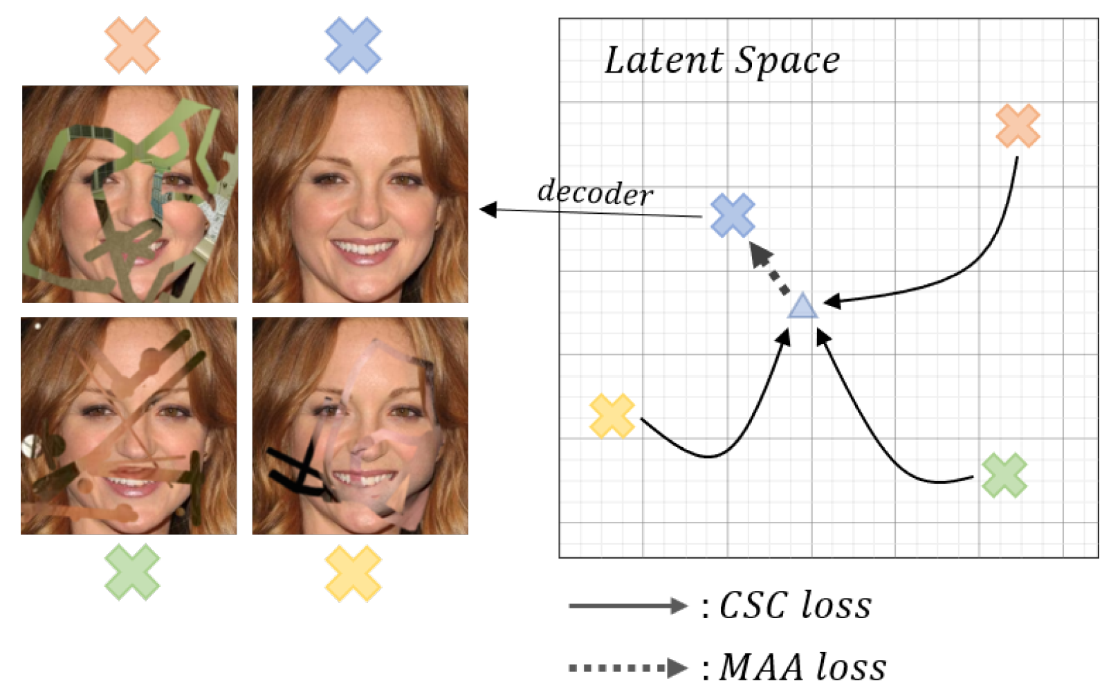
where I represents the identity matrix, and $BCE$ is binary cross-entropy loss. For the convenience of implementation, the complete image is used as one of the degraded images since the complete image can be regarded as a degraded image with an infinitely small noise area. The intuitive explanation of the impact of CSC loss is shown in Figure 3.

3.3.2. Mask-Aware Adversarial Loss (MAA Loss)

Since the parameters of the feature extractor will be updated during training, it cannot be guaranteed that the final latent code is close to the value that represents the complete image when narrowing the distance of all degraded inputs in latent space via CSC loss. We have reasons to speculate that the pulled-closer codes may represent the intermediate states of degraded images, e.g., the average semantic of the training set where the mask frequently appears. Therefore, the pulled-close latent code must be pushed back to the position representing the complete image, as shown in Figure 3.

It is worth noting that the difference between a degraded image and a complete image is that the former can be visually divided into different regions, while the latter cannot. The pushing-back process is to further eliminate the influence of the noise by minimizing the mutual information between the latent representation and the noise. Therefore, we train a mask-aware discriminator to predict the mask from the latent code while training the encoder to extract the latent code from the degraded images that no mask region can be predicted. For more precisely locating the mask region, the latent code is translated to the size of $I_{deg}^L$. Our mask-aware adversarial loss ${\mathcal{L}}_{\mathit{MAA}}$ is:

$$\begin{array}{cc}\hfill {\mathcal{L}}_{\mathit{MAA}}=& E_{\widehat{x}\sim P_{\mathit{degraded}}\left(\widehat{x}\right)}[log(M-D_M\left(E\left(\widehat{x}\right)\right))]+\hfill \\ \hfill & E_{x\sim P_{\mathit{complete}}\left(x\right)}[log{D}_M\left(E\left(x\right)\right)]\hfill \end{array}$$

(2)

The robustness of cross-space contrastive learning relies on the quality of the latent representation. In our framework, this quality is maintained by multiple complementary mechanisms. Specifically, the CSC loss encourages spatially aligned and structurally meaningful features by enforcing high correlation at corresponding locations while suppressing mismatched correlations. The proposed mask-aware adversarial training further reduces degradation-related information in the latent space, making the learned representation more degradation-invariant. Together with the reconstruction, perceptual, and adversarial losses, these designs help stabilize latent learning and improve robustness against degraded inputs.

3.3.3. Other Inpainting Losses

Our settings for other traditional inpainting losses follow [1], including reconstruction loss ${\mathcal{L}}_{L_1}^I$, VGG-based perceptual loss ${\mathcal{L}}_{VGG}^I$, and adversarial loss ${\mathcal{L}}_{adv}$. These losses ensure that the low-resolution inpainting result $I_{inp}^L$ is visually reasonable.

$$\begin{array}{c}\hfill {\mathcal{L}}_{L_1}^I=\left|\right|I_{inp}^L-I_{gt}^L{\left|\right|}_1\end{array}$$

(3)

$$\begin{array}{c}\hfill {\mathcal{L}}_{VGG}^I=\sum _i\left|\right|{\Theta }_i(I_{inp}^L)-{\Theta }_i(I_{gt}^L){\left|\right|}_1\end{array}$$

(4)

$$\begin{array}{cc}\hfill {\mathcal{L}}_{adv}=& E_{\widehat{x}\sim P_{\mathit{degraded}}\left(\widehat{x}\right)}[log(1-D_I\left(\widehat{x}\right))]+\hfill \\ \hfill & E_{x\sim P_{\mathit{complete}}\left(x\right)}[log\left(D_I\left(x\right)\right)]\hfill \end{array}$$

(5)

where ${\Theta }_i$ represents the output of the ith layer of VGG. The overall loss of the inpainting network is:

$$\begin{array}{cc}\hfill {\mathcal{L}}_{\mathit{Inp}}& ={\mathcal{L}}_{L_1}^I+{\lambda }_{VGG}^I{\mathcal{L}}_{VGG}^I+{\lambda }_{adv}{\mathcal{L}}_{adv}+\hfill \\ \hfill & {\lambda }_{CSC}{\mathcal{L}}_{CSC}+{\lambda }_{\mathit{MAA}}{\mathcal{L}}_{\mathit{MAA}}\hfill \end{array}$$

(6)

3.3.4. Refine Losses

The upsampled inpainting result $I_{inp}^H$ concatenated with the conditional masked degraded image $I_{deg}^{\prime }$ is input to the refine network. The coarse inpainting result provides visual rationality and overall consistency; the original image provides high-resolution information of the non-degraded area, including color, textures, etc. The upsampling result is expected to be reasonable as a whole without artifacts. We use L1 reconstruction loss ${\mathcal{L}}_{VGG}^R$ and VGG-based perceptual loss ${\mathcal{L}}_{L_1}^R$ for constraining. The refine loss can be expressed as follows:

$$\begin{array}{c}\hfill {\mathcal{L}}_{\mathit{Ref}}={\lambda }_{L_1}^R{\mathcal{L}}_{L_1}^R+{\lambda }_{VGG}^R{\mathcal{L}}_{VGG}^R\end{array}$$

(7)

The total loss of CSCGAN is:

$$\begin{array}{cc}\hfill {\mathcal{L}}_{all}& ={\mathcal{L}}_{\mathit{Inp}}+{\mathcal{L}}_{\mathit{Ref}}\hfill \end{array}$$

(8)

Although our framework does not rely on explicit mask prediction at inference time, corrupted-region localization is still implicitly performed within the model through mask-aware adversarial learning and discrepancy-based refinement. Specifically, the mask-aware discriminator attempts to recover the corrupted-region mask from the latent representation, which provides an internal localization signal during training and encourages the encoder to distinguish corrupted content from valid structures. In the refinement stage, potentially corrupted regions are further identified by comparing the coarse inpainting result with the degraded input, and the resulting discrepancy is used to construct a conditional masked image for refinement. Therefore, localization in our framework is carried out within the model itself in an implicit and internally guided manner, rather than through a separate segmentation-style mask prediction branch. While this design reduces the dependence on accurate mask supervision and is more suitable for practical blind inpainting scenarios, extremely large-scale or highly structured degradations may still remain more challenging cases.

4. Experimental Results

In this section, we prove the superiority of the blind inpainting method proposed in this paper by comparing it with the state-of-the-art methods on three datasets, including CelebA [33], Places2 [34], and Paris Streetview [35]. We selected CelebA, Places2, and Paris StreetView because they are widely used inpainting benchmarks and provide complementary evaluation scenarios, including aligned facial images, diverse natural scenes, and structured urban street views. We compare it with the following baselines: three SOTA image inpainting models, GMCNN [3], RN [1] and LaMa [5], and a state-of-the-art blind inpainting model, VCNet [10]. The methods are retrained and tested under the same experimental settings if the pretrained model is not open-source. Otherwise, we use a mask prediction network trained via VCNet [10] settings to adapt the model to the blind inpainting task.

4.1. Experimental Settings

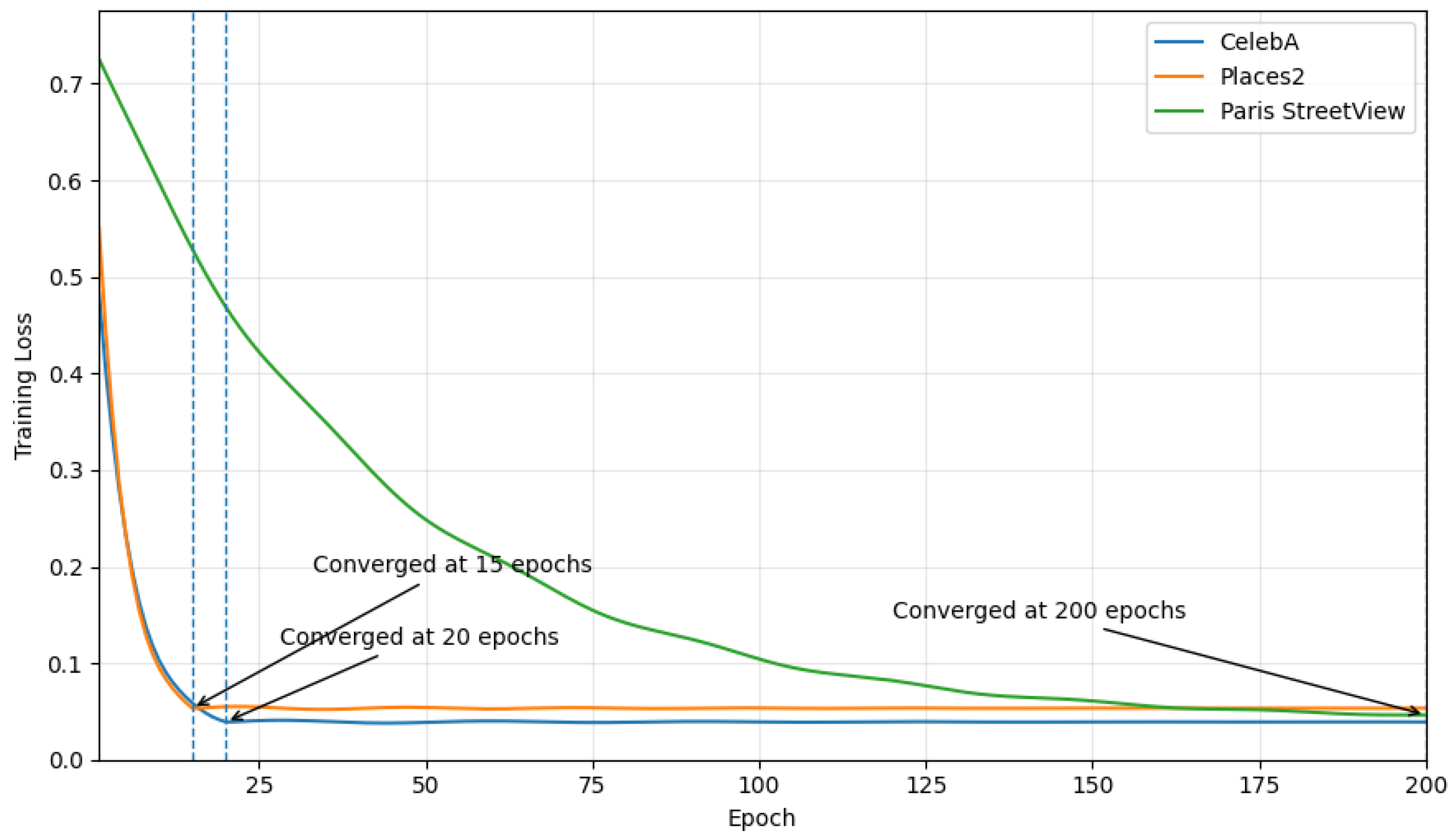
Our method is implemented using PyTorch 1.8.0; the experiment platform is ubuntu16.04. We trained each model on a single NVIDIA RTX 2080Ti GPU with batch size of 12. All experiments are performed on 256 × 256 images. For CelebA, Places2, and Paris Streetview, we separately trained 20, 15, and 200 epochs. These training schedules were determined empirically according to the convergence behavior observed on each dataset. As shown in Figure 4, the training losses become stable around the selected epochs, indicating that these settings are sufficient for convergence. For noise, we mix the hand-drawn mask and automatically generated mask proposed in PConv [36]. After generating the mask dataset, we filter out extreme samples where the mask accounts for less than 10% and more than 85% of the complete image. Gaussian blur with kernel size = 15 is imposed on all masks to produce indistinguishable noise edges. To further ensure the degraded and the non-degraded parts cannot be easily identified by the content, the noisy image is sampled from the same dataset as the ground truth.

4.2. Qualitative Comparison

4.2.1. Compared with General Inpainting Methods

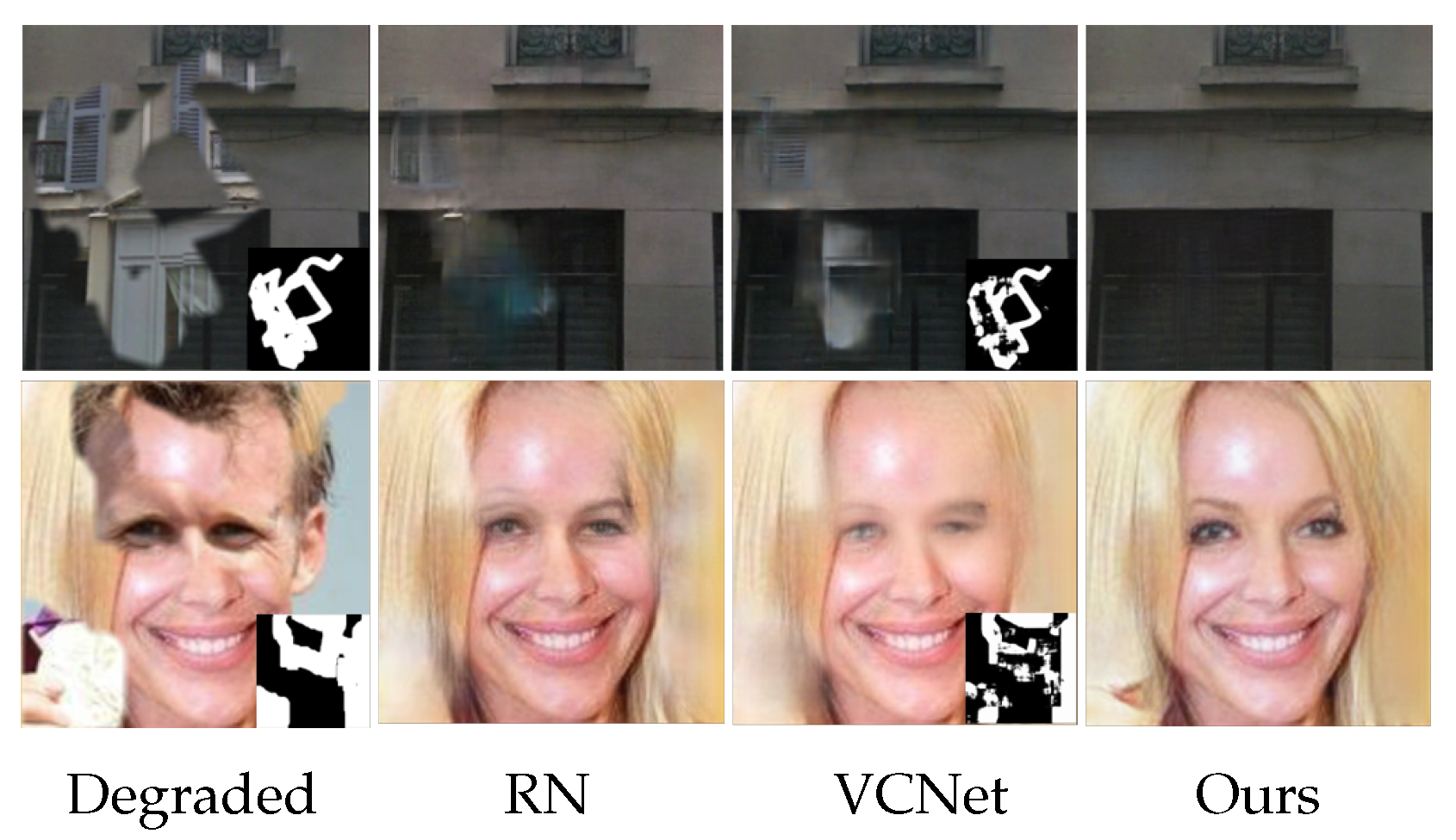
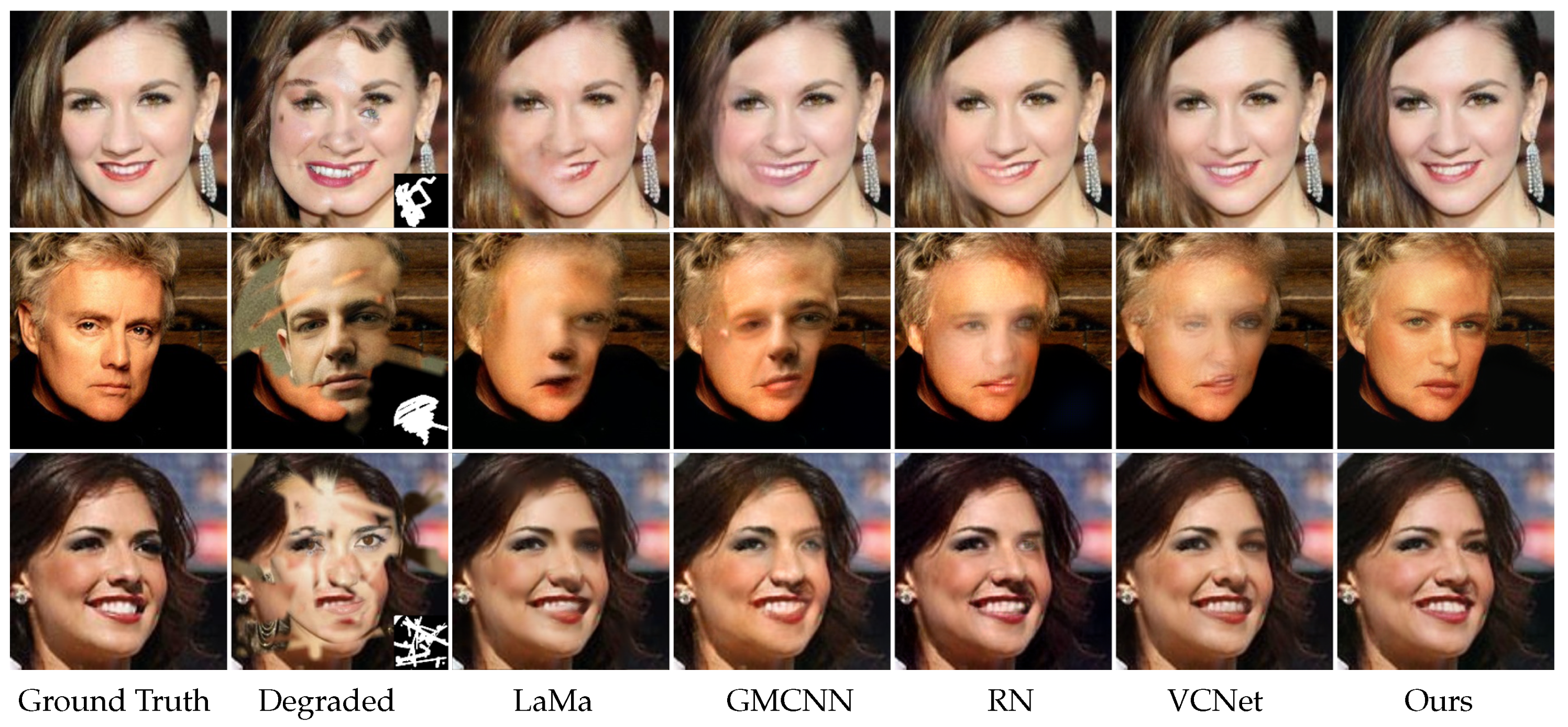
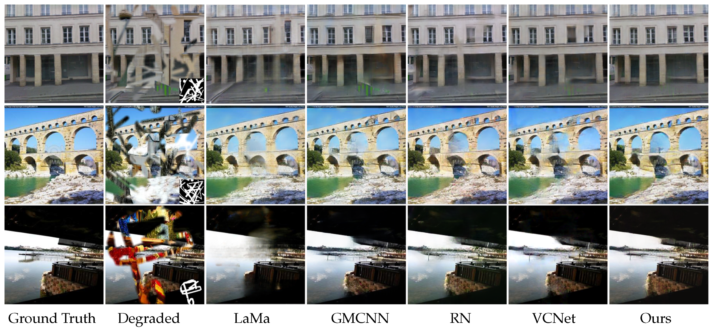
Most previous inpainting networks require precise mask position as guide information. When the mask is not given, the traditional inpainting constraint is not strong enough to drive the model to generate a reasonable and high-quality image. Though the learnable region normalization [1] can sometimes perform well on the blind inpainting task, as shown by the experimental results, it requires users to manually adjust the threshold for different datasets. As Figure 5 and Figure 6 show, our method produces better results in the blind inpainting task than general image inpainting networks. Specifically, our method has fewer artifacts because it removes unreasonable noise content more cleanly. The general inpainting methods cannot separate the noise semantics completely; so, these still retain content of the noise, although that content is unreasonable.

4.2.2. Compared with Blind Inpainting Methods

VCNet [10] transformed the blind inpainting task by introducing a mask prediction module to the general inpainting network. Though the mask-prediction module provides auxiliary information for the inpainting network, it also introduces additional errors. For example, the mask-prediction module usually classifies the content inside the large-area mask as visually reasonable and transmits it to the inpainting network with high confidence. This phenomenon is severe when the noise content and the context are misaligned. The retention of the error content makes the inpainting result of VCNet even worse than the general encoder–decoder network, such as that in [1], in some cases. It can be seen from Figure 7 that the miscalculated mask will make VCNet retain the error information of the noise, e.g., the position of the misplaced human eyes is preserved. Instead, our method can guarantee global rationality (the misplaced eye in Figure 7 is first distinguished and then regenerated), especially for images with fixed structures such as human faces.

4.3. Quantitative Comparison

We apply multiple metrics to our proposed method, the state-of-the-art image inpainting and blind inpainting methods, for quantitative comparison. It is worth noting that, unlike super-resolution, blind inpainting is a highly ill-posed problem. Its purpose is to make the overall perception of the output image reasonable and consistent rather than constraining it to be identical to the ground truth at the pixel level.

The traditional image inpainting evaluation metrics, such as Peak Signal to Noise Ratio (PSNR), Structural Similarity (SSIM), Mean Absolute Error (MAE), etc., generally rely on the statistical information of image pixels, such as mean and variance. But they cannot faithfully reflect the visual rationality of the generated results. Take PSNR as an example: for the inpainting result and the ground truth $I,I_{gt}\in {\mathbb{R}}^{H\times W\times C}$:

$$\begin{array}{c}\hfill \mathit{MSE}={\displaystyle \frac{1}{HWC}}\sum _h\sum _w\sum _c{\left(I(h,w,c)-I_{gt}(h,w,c)\right)}^2\end{array}$$

(9)

$$\begin{array}{c}\hfill \mathit{PSNR}=10·lg({\displaystyle \frac{{\mathit{MAX}}_{h,w}{\left(image\right)}^2}{\mathit{MSE}}})\end{array}$$

(10)

The accurate agreement of most pixels can mask the more significant deviation in the smaller area in the result. An image with a complete structure but with overall weak chromatic aberration or soft blur may be inferior to an image with severe local blur or unreasonable structure in terms of existing metrics.

Based on the above observations, we propose a learning-based Global Consistency Metric (GCM) for the blind inpainting task. We train a commonly used encoder–decoder network for evaluation. The training set uses random noise-contaminated images. Random noise includes local blur, local discoloration, and pixels from other images. The BCE loss is used to constrain the content of the network output noise map to be consistent with the real noise position. The binary mask map $M_{noise}\in {\mathbb{R}}^{H\times W}$ can be regarded as an unreasonable visual area in the image. We binarize the mask map. The pixels with a value of 1 represent the mask area. The metric can be expressed as follows:

$$\begin{array}{c}\hfill \mathit{GCM}={\displaystyle \frac{{\sum }_{h,w}{M}_{noise}}{HW}}\end{array}$$

(11)

Although we have discussed the limitations of statistics-based metrics, they remain effective for assessing the quality of generated images in most cases. Thus, in the comparison of this paper, SSIM is retained. In addition, LPIPS [37] and FID [38] are also used to measure the quality of the inpainting results. Previous studies have shown that these metrics are more stable than those based on Euclidean distance. The detailed quantitative experimental results are shown in

Table 1. Quantitative evaluation of different models on CelebA, Places2, and Paris Streetview datasets. The best results are highlighted in bold. ↑ indicates that higher values are better, while ↓ indicates that lower values are better.

	CelebA				Places2				Paris Streetview
	SSIM ↑	LPIPS ↓	FID ↓	GCM ↓	SSIM ↑	LPIPS ↓	FID ↓	GCM ↓	SSIM ↑	LPIPS ↓	FID ↓	GCM ↓
LaMa [5]	0.85	0.11	16.55	0.16	0.83	0.12	33.25	0.14	0.80	0.18	80.22	0.10
GMCNN [3]	0.84	0.10	18.50	0.20	0.81	0.13	34.72	0.26	0.76	0.21	82.17	0.22
RN [1]	0.86	0.08	16.69	0.15	0.81	0.12	33.52	0.14	0.79	0.18	79.90	0.11
VCNet [10]	0.87	0.10	15.63	0.13	0.80	0.14	34.05	0.15	0.80	0.18	81.38	0.09
CSCGAN w/o CSC loss	0.86	0.09	15.77	0.12	0.79	0.13	33.46	0.15	0.79	0.19	80.05	0.10
CSCGAN w/o MAA loss	0.87	0.07	14.45	0.08	0.82	0.12	33.01	0.12	0.81	0.18	77.64	0.08
CSCGAN	0.88	0.06	13.23	0.05	0.82	0.11	32.89	0.11	0.82	0.17	74.28	0.07

. It can be seen that our method is significantly better than other methods.

4.4. Ablation Studies

4.4.1. W/ and W/O CSC Loss and MAA Loss

As analyzed in Section 3.3 and can be seen in Table 1, CSC loss and MAA loss guarantee the encoder preserves the high-level semantic and resists the influence of the input noise. To prove the effectiveness of our proposed module, we test the distance between the latent code of the ground truth and the degraded image on CelebA. The residual feature distance (RFD) is defined as follows:

$$\begin{array}{c}\hfill \mathit{RFD}=\mathit{sigmoid}(lg(\mathit{MaxPool}\left(\right||E\left(I_{gt}\right)-E\left(I_{deg}\right){\left|\right|}_2\left)\right))\end{array}$$

(12)

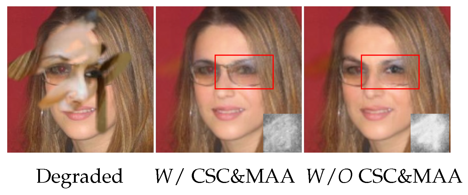
For maxpooling, the kernel size is (Channel, 1, 1). We tested the average distance of the full model and the model without CSC loss and MAA loss. The results were 0.71 and 0.78, respectively. It can be seen in Figure 8 that the model without CSC and MAA loss cannot produce the complete structure of glasses because the noise image does not include the nose support. On the other hand, our full model is more inclined to produce a complete structure, hence producing the nose support based on the semantics of other parts of the glasses.

4.4.2. CSC Loss vs. Latent L1 Loss

CSC loss aims to shorten the distance between the latent code of the degraded image and the ground truth. It is natural to doubt whether the same effect can be achieved by directly applying L1 loss to the corresponding latent codes. We conducted a comparative experiment for this conjecture, and the experimental results proved that directly calculating the L1 loss on the latent code will make the training prone to collapse. This collapse may be due to the instability of the latent code extracted from the ground-truth image. When the encoder is learning to reconstruct and has not yet converged, especially at the first few epochs of training, the gradient of latent L1 loss will change so drastically that it will affect the convergence of the entire GAN. Different from the L1 loss, our CSC loss is a soft constraint; thus, it can provide a more stable training process.

4.4.3. Preservation of Reasonable Areas

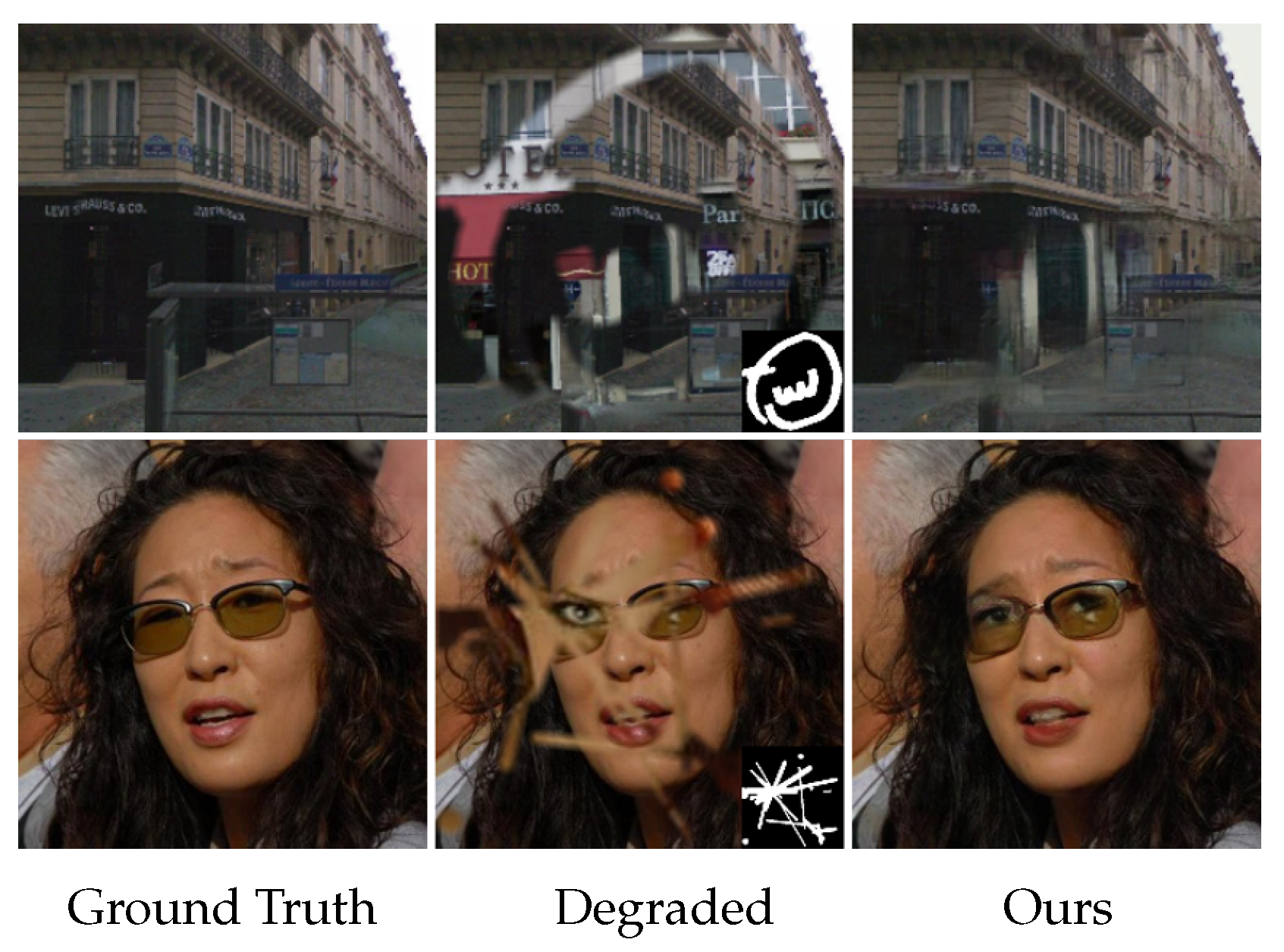
It is found in the experiment that our network can retain some visually reasonable areas of the degraded image, even if these areas come from noise. It requires the content of added noise and the context of the non-degraded area to be highly aligned. This feature gives the network the potential for image editing. As shown in Figure 9, the content of noise can slightly affect the inpainting results. Please note that the white pillars and the open eyes appearing in the inpainting results do not exist in the original images.

4.4.4. Complexity and Computational Cost

To provide a clearer view of the practical efficiency of the proposed CSCGAN, we further report its training complexity and computational cost in

Table 2. Training complexity and computational cost of the proposed two-stage CSCGAN on $256\times 256$ images using a single NVIDIA RTX 2080Ti GPU. The training time is measured with a batch size of 12.

Item	Stage I	Stage II	Overall
Trainable parameters (M)	42.3	6.4	48.7
FLOPs per image (G)	55.8	7.6	63.4
Peak GPU memory (training, GB)	8.7	2.1	9.8
Training time per epoch (min)	27	4	31
Inference time per image (ms)	101	25	126

. Since CSCGAN adopts a two-stage architecture, we separately summarize the complexity of the coarse inpainting network (Stage I) and the refinement network (Stage II), together with the overall cost. As shown in the table, the main computational burden lies in Stage I, which performs the primary blind inpainting process, while Stage II introduces only a relatively small additional overhead for detail refinement. This observation is consistent with our design motivation, where the refinement stage is intentionally kept lightweight. Consistent with the experimental settings described above, all complexity and runtime results are obtained on $256\times 256$ images using a single NVIDIA RTX 2080Ti GPU, and the training time is measured with a batch size of 12.

4.4.5. Other Applications

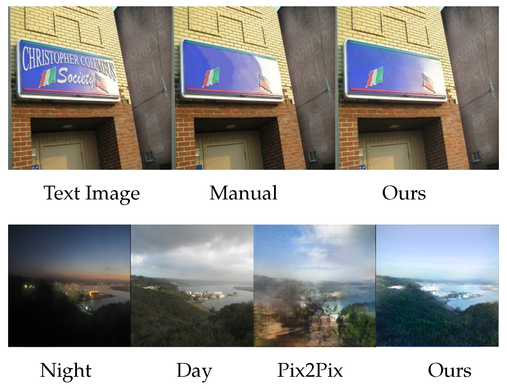
Surprisingly, our method can be directly applied to some other tasks without any additional elaborate design, e.g., text removal and image-to-image translation (I2IT). Since there is no ground-truth mask, the MAA loss degenerates into a general adversarial loss in these tasks. We train our model on SCUT-EnsText [19] and night2day [39] for comparison. As can be seen from Figure 10, our method achieves the same level or even exceeds the baseline on these tasks. In the text removal experiment, our method generates even smoother content in inpainted regions than manually calibrated ground truth.

5. Conclusions

In this paper, an efficient blind image inpainting framework is proposed to generate visually reasonable inpainting results without the need for mask prediction. Two novel constraints are proposed to remove noises from degraded images in the latent space. By the constraint of coupled cross-space contrastive loss and mask-aware adversarial loss, the complete image and its corresponding multiple degraded images are projected to the same position in the latent space, which maximizes the correlation between the inpainting result and the complete image while minimizing the correlation between the inpainting result and the noise. Consequently, the degraded images can be repaired in the latent space. The experiments prove that our method not only achieves SOTA performance on blind inpainting tasks but can also be directly generalized to multiple neighborhood tasks. In real-world blind inpainting scenarios, accurate masks are usually unavailable, and degradation patterns are often irregular and ambiguous. Therefore, our mask-prediction-free framework is more suitable for practical applications, although more extensive evaluation on diverse real-world degradations remains an important direction for future work. To further improve robustness and restoration quality in such scenarios, we plan to investigate additional strategies, such as mapping the latent code into a pretrained decoder space and adopting alternative backbone architectures.

References

1. Yu, T.; Guo, Z.; Jin, X.; Wu, S.; Chen, Z.; Li, W.; Zhang, Z.; Liu, S. Region normalization for image inpainting. Proc. AAAI Conf. Artif. Intell. 2020, 34, 12733–12740. [Google Scholar] [CrossRef] [Scilit]
2. Yu, J.; Lin, Z.; Yang, J.; Shen, X.; Lu, X.; Huang, T.S. Generative image inpainting with contextual attention. In Proceedings of the 2018 IEEE/CVF Conference on Computer Vision and Pattern Recognition, Salt Lake City, UT, USA, 18–23 June 2018; IEEE: Piscataway, NJ, USA, 2018; pp. 5505–5514. [Google Scholar]
3. Wang, Y.; Tao, X.; Qi, X.; Shen, X.; Jia, J. Image inpainting via generative multi-column convolutional neural networks. arXiv 2018, arXiv:1810.08771. [Google Scholar] [CrossRef] [Scilit]
4. Nazeri, K.; Ng, E.; Joseph, T.; Qureshi, F.Z.; Ebrahimi, M. EdgeConnect: Generative Image Inpainting with Adversarial Edge Learning. arXiv 2019, arXiv:1901.00212. [Google Scholar] [CrossRef] [Scilit]
5. Suvorov, R.; Logacheva, E.; Mashikhin, A.; Remizova, A.; Ashukha, A.; Silvestrov, A.; Kong, N.; Goka, H.; Park, K.; Lempitsky, V. Resolution-robust large mask inpainting with fourier convolutions. In Proceedings of the 2022 IEEE/CVF Winter Conference on Applications of Computer Vision (WACV), Waikoloa, HI, USA, 3–8 January 2022; IEEE: Piscataway, NJ, USA, 2022; pp. 2149–2159. [Google Scholar]
6. Zhao, S.; Cui, J.; Sheng, Y.; Dong, Y.; Liang, X.; Chang, E.I.; Xu, Y. Large scale image completion via co-modulated generative adversarial networks. arXiv 2021, arXiv:2103.10428. [Google Scholar] [CrossRef] [Scilit]
7. Liu, Y.; Pan, J.; Su, Z. Deep blind image inpainting. In Intelligence Science and Big Data Engineering, Proceedings of the 9th International Conference, IScIDE 2019, Nanjing, China, 17–20 October 2019; Springer: Cham, Switzerland, 2019; pp. 128–141. [Google Scholar]
8. Chen, H.; Giuffrida, M.V.; Doerner, P.; Tsaftaris, S.A. Blind Inpainting of Large-scale Masks of Thin Structures with Adversarial and Reinforcement Learning. arXiv 2019, arXiv:1912.02470. [Google Scholar] [CrossRef] [Scilit]
9. Wang, J.; Chen, S.; Wu, Z.; Jiang, Y.G. FT-TDR: Frequency-guided Transformer and Top-Down Refinement Network for Blind Face Inpainting. IEEE Trans. Multimed. 2022, 25, 2382–2392. [Google Scholar] [CrossRef] [Scilit]
10. Wang, Y.; Chen, Y.C.; Tao, X.; Jia, J. VCNet: A Robust Approach to Blind Image Inpainting. In Computer Vision—ECCV 2020, Proceedings of the 16th European Conference, Glasgow, UK, 23–28 August 2020; Springer: Cham, Switzerland, 2020. [Google Scholar]
11. Chen, T.; Kornblith, S.; Norouzi, M.; Hinton, G. A simple framework for contrastive learning of visual representations. In Proceedings of the 37th International Conference on Machine Learning; PMLR: Cambridge, MA, USA, 2020; pp. 1597–1607. [Google Scholar]
12. Zbontar, J.; Jing, L.; Misra, I.; LeCun, Y.; Deny, S. Barlow twins: Self-supervised learning via redundancy reduction. arXiv 2021, arXiv:2103.03230. [Google Scholar] [CrossRef] [Scilit]
13. Pathak, D.; Krahenbuhl, P.; Donahue, J.; Darrell, T.; Efros, A.A. Context encoders: Feature learning by inpainting. In Proceedings of the 2016 IEEE Conference on Computer Vision and Pattern Recognition (CVPR), Las Vegas, NV, USA, 27–30 June 2016; IEEE: Piscataway, NJ, USA, 2016; pp. 2536–2544. [Google Scholar]
14. Yang, J.; Qi, Z.; Shi, Y. Learning to incorporate structure knowledge for image inpainting. Proc. AAAI Conf. Artif. Intell. 2020, 34, 12605–12612. [Google Scholar] [CrossRef] [Scilit]
15. Wang, T.; Ouyang, H.; Chen, Q. Image Inpainting with External-internal Learning and Monochromic Bottleneck. arXiv 2021, arXiv:2104.09068. [Google Scholar] [CrossRef] [Scilit]
16. Ko, K.; Kim, C.S. Continuously masked transformer for image inpainting. In Proceedings of the 2023 IEEE/CVF International Conference on Computer Vision (ICCV), Paris, France, 1–6 October 2023; IEEE: Piscataway, NJ, USA, 2023; pp. 13169–13178. [Google Scholar]
17. Li, Z.; Zhang, Y.; Du, Y.; Wang, X.; Wen, C.; Zhang, Y.; Geng, G.; Jia, F. STNet: Structure and texture-guided network for image inpainting. Pattern Recognit. 2024, 156, 110786. [Google Scholar] [CrossRef] [Scilit]
18. Li, Z.; Han, N.; Wang, Y.; Zhang, Y.; Yan, J.; Du, Y.; Geng, G. Image inpainting based on CNN-Transformer framework via structure and texture restoration. Appl. Soft Comput. 2025, 170, 112671. [Google Scholar] [CrossRef] [Scilit]
19. Zhang, S.; Liu, Y.; Jin, L.; Huang, Y.; Lai, S. Ensnet: Ensconce text in the wild. Proc. AAAI Conf. Artif. Intell. 2019, 33, 801–808. [Google Scholar] [CrossRef] [Scilit]
20. Wang, X.; Li, Y.; Zhang, H.; Shan, Y. Towards real-world blind face restoration with generative facial prior. In Proceedings of the 2021 IEEE/CVF Conference on Computer Vision and Pattern Recognition (CVPR), Nashville, TN, USA, 20–25 June 2021; IEEE: Piscataway, NJ, USA, 2021; pp. 9168–9178. [Google Scholar]
21. Zhao, H.; Wang, Y.; Gu, Z.; Zheng, B.; Zheng, H. Context-aware mutual learning for blind image inpainting and beyond. Expert Syst. Appl. 2025, 268, 126224. [Google Scholar] [CrossRef] [Scilit]
22. Chihaoui, H.; Lemkhenter, A.; Favaro, P. Blind image restoration via fast diffusion inversion. Adv. Neural Inf. Process. Syst. 2024, 37, 34513–34532. [Google Scholar]
23. Meng, J.; Liu, W.; Shi, C.; Li, Z.; Liu, J. Self-information and prediction mask enhanced blind inpainting network for dunhuang murals. Eng. Appl. Artif. Intell. 2025, 159, 111769. [Google Scholar] [CrossRef] [Scilit]
24. He, K.; Fan, H.; Wu, Y.; Xie, S.; Girshick, R. Momentum contrast for unsupervised visual representation learning. In Proceedings of the 2020 IEEE/CVF Conference on Computer Vision and Pattern Recognition (CVPR), Seattle, WA, USA, 13–19 June 2020; IEEE: Piscataway, NJ, USA, 2020; pp. 9729–9738. [Google Scholar]
25. Henaff, O. Data-efficient image recognition with contrastive predictive coding. In Proceedings of the International Conference on Machine Learning; PMLR: Cambridge, MA, USA, 2020; pp. 4182–4192. [Google Scholar]
26. Hjelm, R.D.; Fedorov, A.; Lavoie-Marchildon, S.; Grewal, K.; Bachman, P.; Trischler, A.; Bengio, Y. Learning deep representations by mutual information estimation and maximization. arXiv 2018, arXiv:1808.06670. [Google Scholar]
27. Hadsell, R.; Chopra, S.; LeCun, Y. Dimensionality reduction by learning an invariant mapping. In Proceedings of the 2006 IEEE Computer Society Conference on Computer Vision and Pattern Recognition (CVPR’06), New York, NY, USA, 17–22 June 2006; IEEE: Piscataway, NJ, USA, 2006; Volume 2, pp. 1735–1742. [Google Scholar]
28. Dosovitskiy, A.; Springenberg, J.T.; Riedmiller, M.; Brox, T. Discriminative unsupervised feature learning with convolutional neural networks. In Advances in Neural Information Processing Systems; Curran Associates, Inc.: Red Hook, NY, USA, 2014. [Google Scholar]
29. Park, T.; Efros, A.A.; Zhang, R.; Zhu, J.Y. Contrastive learning for unpaired image-to-image translation. In Computer Vision—ECCV 2020, Proceedings of the 16th European Conference, Glasgow, UK, 23–28 August 2020; Springer: Springer: Cham, Switzerland, 2020; pp. 319–345. [Google Scholar]
30. Chopra, S.; Hadsell, R.; LeCun, Y. Learning a similarity metric discriminatively, with application to face verification. In Proceedings of the 2005 IEEE Computer Society Conference on Computer Vision and Pattern Recognition (CVPR’05), San Diego, CA, USA, 20–25 June 2005; IEEE: Piscataway, NJ, USA, 2005; Volume 1, pp. 539–546. [Google Scholar]
31. Wu, G.; Jiang, J.; Jiang, K.; Liu, X. Learning from history: Task-agnostic model contrastive learning for image restoration. Proc. AAAI Conf. Artif. Intell. 2024, 38, 5976–5984. [Google Scholar] [CrossRef] [Scilit]
32. Wang, Z.; Peng, J.; Zhao, H.; Yao, L.; Zhao, K. Orthogonal Decoupling Contrastive Regularization: Towards Uncorrelated Feature Decoupling for Unpaired Image Restoration. IEEE Trans. Pattern Anal. Mach. Intell. 2025, 48, 1842–1859. [Google Scholar] [CrossRef] [Scilit] [PubMed]
33. Lee, C.H.; Liu, Z.; Wu, L.; Luo, P. MaskGAN: Towards Diverse and Interactive Facial Image Manipulation. In Proceedings of the 2020 IEEE/CVF Conference on Computer Vision and Pattern Recognition (CVPR), Seattle, WA, USA, 13–19 June 2020; IEEE: Piscataway, NJ, USA, 2020. [Google Scholar]
34. Zhou, B.; Lapedriza, A.; Khosla, A.; Oliva, A.; Torralba, A. Places: A 10 million image database for scene recognition. IEEE Trans. Pattern Anal. Mach. Intell. 2017, 40, 1452–1464. [Google Scholar] [CrossRef] [Scilit] [PubMed]
35. Doersch, C.; Singh, S.; Gupta, A.; Sivic, J.; Efros, A. What makes Paris look like Paris? ACM Trans. Graph. 2012, 31, 101. [Google Scholar] [CrossRef]
36. Liu, G.; Reda, F.A.; Shih, K.J.; Wang, T.C.; Tao, A.; Catanzaro, B. Image inpainting for irregular holes using partial convolutions. In Computer Vision—ECCV 2018, Proceedings of the 15th European Conference, Munich, Germany, 8–14 September 2018; Springer: Cham, Switzerland, 2018; pp. 85–100. [Google Scholar]
37. Zhang, R.; Isola, P.; Efros, A.A.; Shechtman, E.; Wang, O. The unreasonable effectiveness of deep features as a perceptual metric. In Proceedings of the 2018 IEEE/CVF Conference on Computer Vision and Pattern Recognition, Salt Lake City, UT, USA, 18–23 June 2018; IEEE: Piscataway, NJ, USA, 2018; pp. 586–595. [Google Scholar]
38. Heusel, M.; Ramsauer, H.; Unterthiner, T.; Nessler, B.; Hochreiter, S. Gans trained by a two time-scale update rule converge to a local nash equilibrium. In Proceedings of the 31st Conference on Neural Information Processing Systems (NIPS 2017), Long Beach, CA, USA, 4–9 December 2017; Neural Information Processing Systems Foundation, Inc.: Long Beach, CA, USA, 2017; Volume 30. [Google Scholar]
39. Isola, P.; Zhu, J.Y.; Zhou, T.; Efros, A.A. Image-to-image translation with conditional adversarial networks. In Proceedings of the 2017 IEEE Conference on Computer Vision and Pattern Recognition (CVPR), Honolulu, HI, USA, 21–26 July 2017; IEEE: Piscataway, NJ, USA, 2017; pp. 1125–1134. [Google Scholar]
Figure 1. Exemplar blind inpainting results of our method on natural scenes (column one), human faces (column two), scene with text (column three, top), and artwork (column three, bottom). For each set of samples, (left): degraded image, (right): inpainting result. The fifth image from the left in the first row contains Chinese characters on the street sign, which are part of the original scene text and denote a street name.
Applsci 16 02969 g001
Figure 2. Overview of our blind inpainting framework with the two-stage network. The inpainting network is responsible for repairing the degraded images. The refine network is responsible for refining the coarse inpainting results from the inpainting network.
Applsci 16 02969 g002
Figure 3. An intuitive display of how CSC loss and MAA loss affect in the latent space. The four colored crosses represent the latent code of the complete image and the corresponding three different degraded images without our proposed losses. CSC loss makes different degraded images mapped to the same position, while MAA loss makes their position closer to that of the complete image.
Applsci 16 02969 g003
Figure 4. Training loss curves on CelebA, Places2, and Paris StreetView. The losses gradually converge and become stable around 20, 15, and 200 epochs, respectively, providing empirical support for the selected training schedules.
Applsci 16 02969 g004
Figure 5. Comparisons on human faces for blind inpainting. The corresponding noise position is in the lower right corner of the degraded image for better reference. For each group of samples, the size of the mask does not exceed half of the image size.
Applsci 16 02969 g005
Figure 6. Comparisons on street view and natural scenes for blind inpainting. The corresponding noise position is in the lower right corner of the degraded image for better reference.
Applsci 16 02969 g006
Figure 7. Inpainting results of large-area content dislocation noise. The ground-truth mask and the mask predicted by VCNet are shown in the lower right corner of the corresponding samples.
Applsci 16 02969 g007
Figure 8. Comparison between models W/ and W/O CSC loss and MAA loss (with the corresponding residual feature map at the right bottom). The tested models were trained on CelebA for 20 epochs.
Applsci 16 02969 g008
Figure 9. Image editing on street view and human face. From left to right: the ground truth, the degraded image (with the mask at the right bottom) and the inpainting result of our model.
Applsci 16 02969 g009
Figure 10. Other applications. First row: text removal result. Our method generates smoother content than the manually calibrated one. Second row: I2IT result. After the same epochs of training, our method can generate cleaner samples than the baseline.
Applsci 16 02969 g010