Temperature Control of Thermal Performance Testing Systems Based on an Adaptive PI–RLS–MPC Strategy

Abstract

Accurate thermal conductivity measurement requires temperature control systems to establish stable operating conditions within a limited time. In practical thermal conductivity performance testing systems, large thermal inertia, complex heat transfer paths, and input time delays arising from thermal propagation and sensor placement often degrade dynamic response and control accuracy. To overcome these limitations, a composite PI–RLS–MPC control strategy is proposed for thermal systems with inertia and time delay. A proportional–integral (PI) controller serves as the baseline stabilizing controller, while model predictive control (MPC) is utilized to optimize the control input by explicitly considering system delay and input constraints. To enhance robustness against model uncertainty and parameter variations, recursive least squares (RLS) is adopted for online parameter identification and adaptive PI tuning, and a steady-state parameter freezing mechanism is introduced to suppress unnecessary parameter updates after convergence. Simulation studies are performed on an identified thermal process model with a 20 s input time delay. The results indicate that the proposed strategy reduces overshoot, shortens settling time, and improves disturbance rejection compared with conventional controllers. Overall, the proposed PI–RLS–MPC approach provides a practical solution for improving temperature control performance in thermal conductivity testing systems.

1. Introduction

The thermal conductivity of materials is a key physical parameter that characterizes heat transfer capability and plays an important role in a wide range of applications, including electronic thermal management, aerospace engineering, building insulation, and energy equipment. With the increasing demand for higher accuracy in industrial and material testing, thermal conductivity measurement systems are required to establish stable operating conditions within a shorter time to ensure reliable thermal conductivity measurements. However, practical heating systems usually involve complex heat transfer paths and large thermal inertia. Moreover, due to factors such as sensor placement, a significant time delay commonly exists between the control input and the measured temperature response, making it difficult for the system to reach the target temperature rapidly and stably [1,2,3].

Conventional PID control is widely used in temperature control systems owing to its simple structure and ease of implementation. Nevertheless, in heating processes with pronounced thermal inertia and time-delay characteristics, traditional PID controllers struggle to achieve a satisfactory balance between dynamic response speed and steady-state accuracy [4]. To improve control performance, various methods such as feedforward compensation, fuzzy control, and Smith predictor-based approaches have been proposed [5,6,7]. These methods, however, generally rely on empirical design or accurate process models, and their performance may deteriorate under operating condition variations and model uncertainties. In recent years, intelligent algorithms, including genetic algorithms, particle swarm optimization, and neural networks, have been applied to controller parameter tuning, providing certain performance improvements [8,9,10,11]. Despite this, their dependence on training data and computational resources limits their practical engineering applications.

Model predictive control (MPC) explicitly predicts future system behavior using a process model and employs a receding horizon control strategy with feedback correction, offering clear advantages in handling time-delay systems and input constraints [12,13]. Since MPC inherently possesses predictive capability, its function partially overlaps with the derivative action in traditional PID control. To avoid prediction redundancy and noise amplification, a proportional–integral (PI) controller is adopted as the baseline stabilizing controller, while MPC is introduced to supervise and optimize the control input [14,15]. Furthermore, to address model uncertainty and time-varying parameters, recursive least squares (RLS) is incorporated for online parameter identification and adaptive adjustment [16], resulting in a composite PI–RLS–MPC control strategy aimed at improving the dynamic performance, steady-state accuracy, and robustness of thermal systems with inertia and time delay.

The main contributions of this work are summarized as follows.

• A hierarchical PI–RLS–MPC composite control architecture is developed, in which PI provides baseline stabilization, MPC performs predictive supervisory optimization under input constraints, and RLS is used to adaptively tune the PI parameters online. The separation of functions among these three layers allows different time-scale regulation of the system dynamics [17,18,19,20,21,22,23].
• The proposed method introduces an indirect learning mechanism between MPC and RLS. In most conventional adaptive MPC approaches, recursive identification algorithms are used to estimate plant model parameters and update the prediction model used by MPC. In contrast, the proposed framework keeps the MPC prediction model fixed, while the RLS algorithm adjusts the PI controller parameters instead of the plant model parameters. The control increment generated by MPC is used as the learning signal, allowing the PI controller to gradually approximate the optimized control behavior suggested by MPC.
• A steady-state parameter freezing mechanism based on error-band detection is designed. When the system output enters a predefined steady-state tolerance band, the RLS adaptation is automatically deactivated to avoid unnecessary parameter drift and steady-state oscillations.

Therefore, the contribution of this work lies in the coordinated control framework and adaptive interaction mechanism among PI, MPC, and RLS rather than the individual control algorithms themselves.

2. System Modeling and Control Strategy

2.1. System Modeling and Model Identification

2.1.1. Measurement Principle of the System

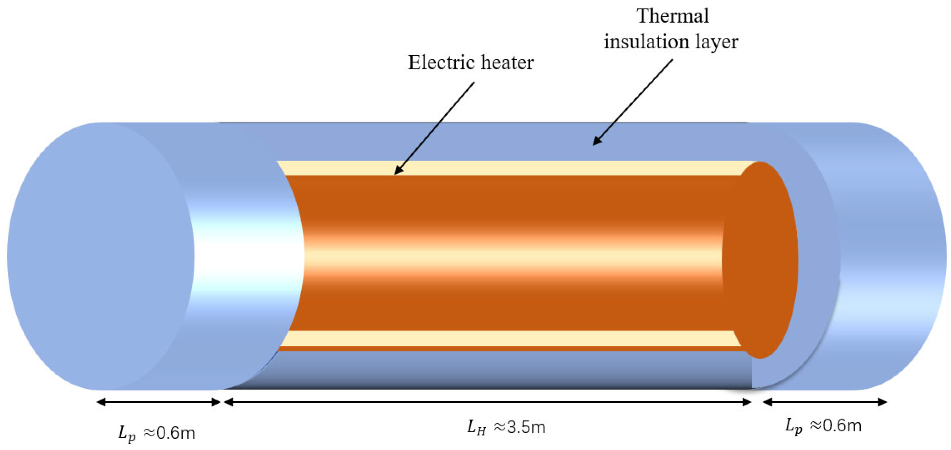
Taking a cylindrical thermal conductivity testing system as an example, the objective is to ensure that the temperature of the external thermal insulation layer rapidly reaches the desired setpoint with minimal oscillations, thereby maintaining a stable and constant temperature. The schematic diagram of the system is shown in Figure 1.

In the sealed cylindrical tube, heat is generated by the circular electric heater located in the main heating section. The generated heat is first transferred to the enclosed air inside the tube and then conducted to the inner wall of the metal tube. Subsequently, the heat propagates through the tube wall to the surrounding thermal insulation layer and is finally dissipated to the ambient environment.

The left and right thermal protective sections, each with a length of $L_p$ ≈ 0.6 m, are heated synchronously to ensure that heat transfer in the central measurement section occurs predominantly in the radial direction. Under thermal equilibrium conditions, the temperature of the thermal insulation layer remains constant, the energy stored within the system does not change, and the electrical heating power is equal to the heat transferred to the environment through the insulation material. Let $P$ denote the heating power generated by the electric heater. Under steady-state conditions, the heat conduction through the cylindrical thermal insulation layer can be expressed as

$$P={\displaystyle \frac{2\pi Lk\mathrm{∆}T}{\mathit{ln}(\frac{r_o}{r_i})}}$$

(1)

where $r_i$ and $r_o$ represent the inner and outer radii of the thermal insulation layer. $L_H$ is the effective length of the central measurement section, which is approximately 3.5 m. $\mathrm{∆}T$ is the steady-state temperature difference between the inner and outer surfaces of the thermal insulation layer, which can be measured using thermocouples. The thermal insulation layer is made of rock wool. Under steady-state conditions, all parameters except the thermal conductivity $k$ are known, and therefore, the thermal conductivity $k$ of the thermal insulation material can be calculated [24,25,26].

2.1.2. Derivation of the Heat Transfer Model

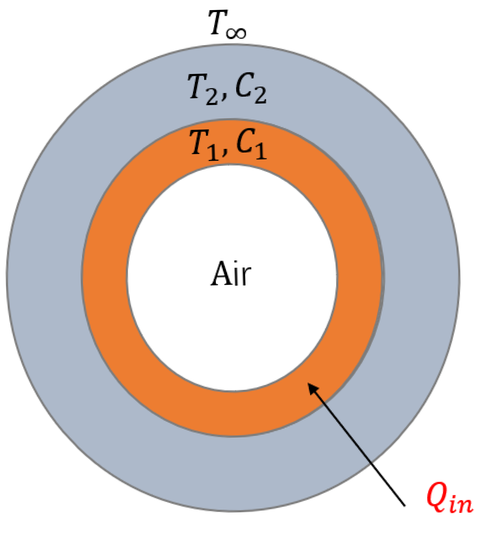
To construct an engineering-oriented model suitable for system identification and control design, a lumped-parameter approach is adopted in this study. The thermal system is equivalently represented by two temperature nodes, namely, the internal air temperature together with the inner wall temperature and the thermal insulation material temperature [27,28]. The corresponding cross-sectional view of the heat transfer structure in the measurement section is illustrated in Figure 2.

Define the temperature rise variables as

$${\theta }_1\left(t\right)=T_1\left(t\right)-T_{\infty }$$

(2)

$${\theta }_2\left(t\right)=T_2\left(t\right)-T_{\infty }$$

(3)

${\theta }_1$ denotes the temperature difference between the internal air together with the inner wall temperature $T_1$ and the ambient temperature $T_{\infty }$, while ${\theta }_2$ represents the temperature difference between the thermal insulation layer temperature $T_2$ and the ambient temperature $T_{\infty }$. At node 1 (internal air and inner wall), the following relation holds:

$$C_1{\displaystyle \frac{d{\theta }_1}{dt}}=Q_{in}\left(t\right)-{\displaystyle \frac{T_1-T_2}{R_1}}$$

(4)

where $C_1$ denotes the thermal capacitance of node 1, $Q_{in}\left(t\right)$ represents the heating power input of the electric heater, and $R_1$ is the thermal resistance between node 1 and node 2 (the thermal insulation layer). Similarly, at node 2,

$$C_2{\displaystyle \frac{d{\theta }_2}{dt}}={\displaystyle \frac{T_1-T_2}{R_1}}-{\displaystyle \frac{{\theta }_2}{R_2}}$$

(5)

where $C_2$ denotes the thermal capacitance of node 2, and $R_2$ is the thermal resistance from the inner surface of the thermal insulation layer to the ambient t. By applying the Laplace transform to the above equations and eliminating the intermediate variables, the model can be reformulated as:

$$G\left(S\right)={\displaystyle \frac{{\theta }_2\left(s\right)}{Q_{in}\left(s\right)}}={\displaystyle \frac{K}{a_2{s}^2+a_{1}s+1}}$$

(6)

where $K$ = $R_2$, $a_2$ = $C_1{C}_2{R}_1{R}_2$ and $a_1$ = $C_1{R}_1+C_1{R}_2+C_2{R}_2$. By taking the input time delay into account, the final transfer function can be expressed as:

$$G\left(S\right)={\displaystyle \frac{K}{a_2{s}^2+a_{1}s+1}}{e}^{-\tau s}$$

(7)

2.1.3. Model’s Identification and Validation

A step heating power of 300 W was applied to the system, and the corresponding temperature response data were collected for model identification. The least squares method was employed [28,29], in which the error between the experimental temperature measurements and the model-predicted values was defined as the objective function.

$$J=\sum _i^N{({\theta }_2,\mathit{exp}(t_i)-{\theta }_2,\mathit{mod}el\left(t_i\right))}^2$$

(8)

where $N$ is the total number of sampling points, and $t_i$ denotes the sampling time at index $i$. By minimizing this objective function through numerical optimization, the optimal model parameters were obtained as $K$ = 0.41, $a_2$ = 263, $a_1$ = 463, and $\tau$ = 20 s. Substituting these parameters into the model, the transfer function can be expressed as

$$G\left(S\right)={\displaystyle \frac{0.41}{263s^2+463s+1}}{e}^{-20s}$$

(9)

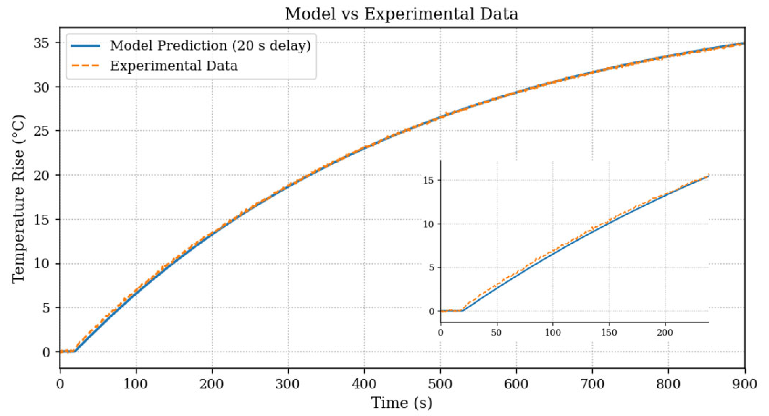
The comparison between the identified model output and the experimental temperature response, and a zoomed view of the initial response, is shown in Figure 3.

As shown in Figure 3, the temperature remains nearly unchanged during the first 0–20 s, which is consistent with the identified input time delay. After 20 s, the rising stage, inflection behavior, and steady-state value of the model output closely match the experimental data, indicating a high degree of agreement between the model and the real system.

2.2. Control Strategy of the System

During operation, the cylindrical insulation heating device exhibits typical characteristics such as thermal inertia, pronounced time delay, and parameter uncertainty. The heating power supplied by the electric heater does not immediately cause a change in the thermal insulation layer temperature; instead, the temperature response appears gradually after a certain heat transfer process. This time-delay characteristic makes it difficult for conventional control methods to achieve a satisfactory balance between rapid response and stability.

This chapter focuses on the cylindrical insulation heating system and develops a composite control framework integrating PI control, RLS-based parameter adaptation, and MPC optimization. The objective of this design is to achieve stable and rapid temperature regulation while effectively addressing time delay, actuator constraints, and parameter variations in the thermal process.

2.2.1. State-Space Model of the Plant

Since MPC solves the control problem based on a state-space formulation, it is necessary to convert the identified transfer function into a state-space model. Under the sampling period $T_S$, the system is discretized, and the resulting discrete-time state-space model with time delay can be expressed as:

$$x\left(k+1\right)=Ax\left(k\right)+Bu\left(k-d\right)$$

(10)

$$y\left(k\right)=Cx\left(k\right)$$

(11)

Here, $d=20/T_s$ denotes the number of discrete steps corresponding to the time delay, $u\left(k\right)$ is the heating power input, and the state vector $x\left(k\right)$ represents the system states at time $k$. The state vector can therefore be expressed as

$$x\left(k\right)=\left[\begin{array}{c}{x}_1\left(k\right)\\ x_2\left(k\right)\end{array}\right]=\left[\begin{array}{c}y\left(k\right)\\ y\left(k-1\right)\end{array}\right]$$

(12)

which are defined as the current output and the previous output, and $y\left(k\right)$ is the thermal insulation layer temperature. The system matrices $A$, $B$, and $C$ are given by

$$A=\left[\begin{array}{cc}-a_1& -a_2\\ 1& 0\end{array}\right], B=\left[\begin{array}{c}K(1+a_1+a_2)\\ 0\end{array}\right],C=\left[\begin{array}{cc}1& 0\end{array}\right]$$

(13)

where $A$, $B$, and $C$ are the discrete-time state-space matrices obtained from the identified transfer function parameters $a_1$, $a_2$, and $K$. Due to the presence of a time delay, the current system state is not directly affected by the current control input but is determined by past inputs, which introduces difficulties in the implementation of predictive control. To address this issue in MPC design, a delay-compensation state augmentation approach is adopted, in which past input variables are incorporated into the system state vector [17,30].

Let the original state dimension of the system be $n$, and define the augmented state vector as:

$$\overline{x}\left(k\right)=\left[\begin{array}{c}x\left(k\right)\hfill \\ u(k-1)\hfill \\ u(k-2)\hfill \\ \dots \hfill \\ u(k-d)\hfill \end{array}\right]$$

(14)

The newly added state components are introduced to store the historical inputs that have not yet taken effect on the system output. Based on the input-shifting relationship, the augmented state-space system can be constructed as:

$$\overline{x}\left(k+1\right)=\overline{A}\overline{x}\left(k\right)+\overline{B}u\left(k\right)$$

(15)

$$y\left(k\right)=\overline{C}\overline{x}\left(k\right)$$

(16)

The system matrices $\overline{A}$, $\overline{B}$, and $\overline{C}$ are given by

$$\begin{gathered} A=\left[\begin{array}{cccccc}-a_1& -a_2& 0& \dots & 0& K\left(1+a_1+a_2\right)\\ 1& 0& 0& \dots & 0& 0\\ 0& 0& 0& \dots & 0& 0\\ 0& 0& 1& \dots & 0& 0\\ ⋮& ⋮& ⋮& \ddots & ⋮& ⋮\\ 0& 0& 0& \dots & 1& 0\end{array}\right], B=\left[\begin{array}{c}0\\ 0\\ 1\\ 0\\ ⋮\\ 0\\ 0\end{array}\right] \\ C=\left[\begin{array}{ccccc}1& 0& 0& \dots & 0\end{array}\right] \end{gathered}$$

(17)

where the augmented matrices $\overline{A}$, $\overline{B}$, and $\overline{C}$ are constructed from the original system matrices $A$, $B$, and $C$ by introducing the delayed input states. In the augmented model, the current input $u\left(k\right)$ directly participates in the state update, thereby transforming the original time-delay system into an equivalent higher-dimensional system without explicit time delay. This formulation provides a suitable foundation for the implementation of model predictive control [21,31,32].

2.2.2. Overall Control Design of the System

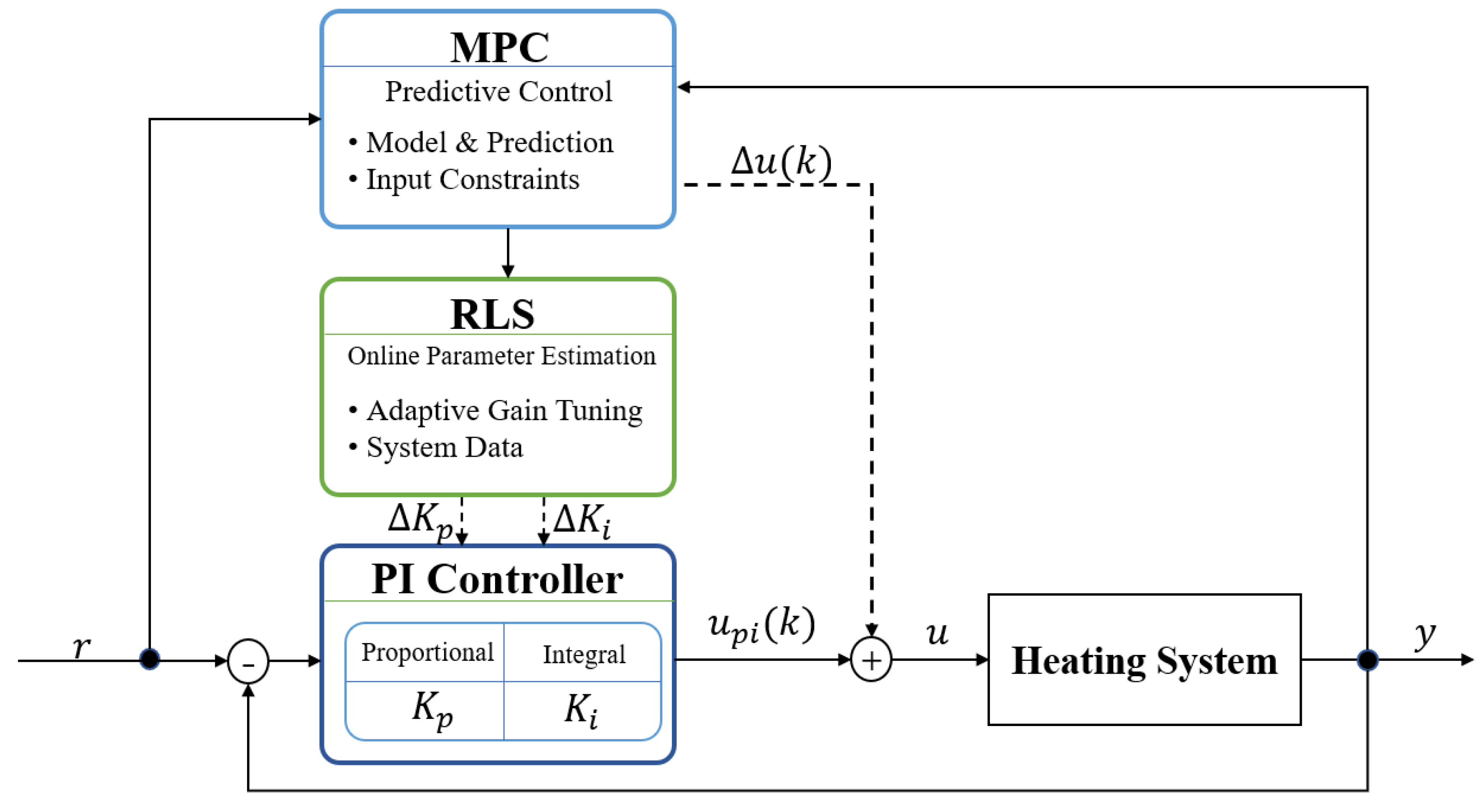
To ensure that the system output temperature $y\left(k\right)$ can reach the reference temperature $r\left(k\right)$ rapidly and smoothly and enter the steady-state error band, a hierarchical composite control architecture is adopted in this study according to the system characteristics. The overall control concept is described as follows in Figure 4.

The lower layer employs a PI controller to provide basic closed-loop stability and steady-state accuracy, forming the foundation of the entire control system. A PI controller is selected instead of a PID controller as the nominal low-level controller because introducing both the derivative term and MPC in a composite control framework may lead to redundancy in predictive functionality and even potential control conflicts. Moreover, the derivative term is highly sensitive to measurement noise, which can amplify noise and degrade the effectiveness of predictive optimization in thermal systems with significant time delay and large thermal inertia. In contrast, the PI controller features a simple structure and smooth control output, providing a stable and reliable baseline control signal for the upper-layer MPC, and is, therefore, more suitable for coordination with MPC.

The upper layer adopts MPC to perform online optimization based on the system model and future prediction information. Under the premise of satisfying input constraints, MPC supervises and adjusts the control output of the PI controller, thereby improving the dynamic response performance of the system. MPC explicitly predicts the future system output over a finite prediction horizon using the identified model and determines the optimal control sequence by solving a constrained optimization problem in a receding horizon manner. Through this mechanism, the control input can be adjusted proactively according to the predicted system behavior, which effectively reduces overshoot, accelerates the transient response, and enhances constraint-handling capability compared with conventional feedback control.

The intermediate layer introduces a RLS module to adjust the PI controller parameters online based on real-time operating data of the system, thereby compensating for model uncertainty and operating condition variations.

In the proposed hierarchical structure, the PI controller provides the baseline feedback regulation, while the MPC module generates a supervisory corrective increment. The actual control input applied to the plant is defined as:

$$u\left(k\right)=u_{PI}\left(k\right)+\mathrm{∆}{u}_{MPC}\left(k\right)$$

(18)

where $u_{PI}\left(k\right)$ is the control signal generated by the lower-layer PI controller and $\mathrm{∆}{u}_{MPC}\left(k\right)$ is the corrective control increment obtained from the MPC optimization. In contrast, the RLS module does not directly modify the plant input but gradually updates the PI parameter vector according to the discrepancy between the PI control increment and the MPC reference increment. Since the MPC layer provides fast corrective action and the RLS adaptation operates on a slower time scale, the control layers interact cooperatively rather than generating conflicting control actions.

2.2.3. Design of the MPC Controller

Based on the augmented model, the one-step-ahead prediction can be expressed as:

$$\overline{x}\left(k+1\left|k\right.\right)=\overline{A}\overline{x}\left(k\right)+\overline{B}u\left(k\right)$$

(19)

$$\widehat{y}\left(k+1\left|k\right.\right)=\overline{C}\overline{x}\left(k+1\left|k\right.\right)$$

(20)

Similarly, the two-step-ahead prediction can be expressed as:

$$\overline{x}\left(k+2\left|k\right.\right)=\overline{A}\overline{x}\left(k+1\left|k\right.\right)+\overline{B}u\left(k+1\right)$$

(21)

$$\widehat{y}\left(k+2\left|k\right.\right)=\overline{C}\overline{x}\left(k+2\left|k\right.\right)$$

(22)

By recursion, the prediction can be extended to $N_p$ steps ahead as:

$$\widehat{Y}\left(k\right)=\left[\begin{array}{c}\widehat{y}(k+1\left|k\right.)\hfill \\ \dots \hfill \\ \widehat{y}(k+N_p\left|k\right.)\hfill \end{array}\right]$$

(23)

Based on the desired temperature $r$ and the tracking error $e$, the reference trajectory $r\left(k+1\right)$ can be expressed as:

$$r\left(k+i\right)=r\left(k\right)+\left(1-e^{-\beta i}\right)\left(r-r\left(k\right)\right),i=\mathrm{1,2},\dots ,N_p$$

(24)

The reference trajectory is designed as a smooth curve, where the parameter $\beta$ determines the rising speed of the trajectory and is typically chosen within the range of 0.05 to 0.3; the initial reference value $r\left(k\right)$ is set equal to the current temperature of the system. The reference trajectory can be expressed in vector form as:

$$R(k)=\left[\begin{array}{c}r(k+1)\hfill \\ \dots \hfill \\ r(k+N_p)\hfill \end{array}\right]$$

(25)

Similarly, the prediction error can be expressed as:

$$E_p(k)=\widehat{Y}(k)-R(k)$$

(26)

To enable MPC to act on the control input in an incremental form, an incremental variable $\mathrm{∆}u\left(k\right)$ is introduced.

$$\mathrm{∆}u\left(k\right)=u\left(k\right)-u(k-1)$$

(27)

Since the above reference quantities are expressed in vector form, the optimization variables of MPC over the control horizon $N_c$ can be defined as:

$$\mathrm{∆}U(k)=\left[\begin{array}{c}\mathrm{∆}u\left(k\right)\hfill \\ \mathrm{∆}u(k+1)\hfill \\ \dots \hfill \\ \mathrm{∆}u(k+N_c-1)\hfill \end{array}\right]$$

(28)

In an error-driven form [33], the objective function can be expressed as:

$$J\left(k\right)=E_p^T\left(k\right)Q\left(k\right)E_p\left(k\right)+\mathrm{∆}{U}^T\left(k\right)P\left(k\right)\mathrm{∆}U\left(k\right)$$

(29)

where $Q\ge 0$ is the output-error weighting matrix that penalizes the tracking error, and $P>0$ is the control weighting matrix that penalizes the control increment. A larger $Q$ emphasizes faster error reduction, whereas a larger $P$ yields smoother control actions by suppressing excessive changes in the input at the cost of a slower response [21,32]. The output weighting matrix $Q$ and the control weighting matrix $P$ are designed as:

$$Q\left(k\right)=Q_0(1+\gamma \left|e\left(k\right)\right|)$$

(30)

$$P(k)={\displaystyle \frac{P_0}{1+\gamma \left|e\left(k\right)\right|}}$$

(31)

The constants $Q_0$ and $P_0$ are the nominal weighting coefficients used to construct the adaptive weighting matrices $Q\left(k\right)$ and $P\left(k\right)$. They determine the baseline trade-off between tracking accuracy and control effort in the MPC objective function. Specifically, a larger $Q_0$ places greater emphasis on reducing the tracking error, resulting in faster error convergence but potentially larger control actions. In contrast, a larger $P_0$ increases the penalty on the control increment, leading to smoother control inputs but possibly slower system responses. where $\gamma$ is the error coefficient that adjusts the sensitivity of the weighting matrices to the tracking error. A larger $\gamma$ increases the influence of the error on $Q\left(k\right)$ and $P\left(k\right)$, leading to more aggressive control when the error is large and more conservative behavior as the error decreases.

The constraints of the objective function can be expressed as:

$$u_{min}\le u\left(k-1\right)+\sum _{j=0}^i\mathrm{∆}u(k+j)\le u_{max}$$

(32)

$$-\mathrm{∆}{u}_{max}^{MPC}\le \mathrm{∆}u(k+i)\le \mathrm{∆}{u}_{max}^{MPC}$$

(33)

Under the above conditions, the optimal solution can be obtained by solving a quadratic programming (QP) problem. According to the receding horizon principle, only the first control action is applied to the system.

$$\mathrm{\Delta }{u}_{MPC}\left(k\right)=\mathrm{∆}{u}_{MPC}^{*}\left(k\right)$$

(34)

where $\mathrm{∆}{u}_{MPC}^{*}\left(k\right)$ denotes the optimal control increment generated by the MPC optimization. When the tracking error satisfies $\left|e\left(k\right)\right|\le {\epsilon }_{MPC}$, the MPC control increment is set to $\mathrm{∆}{u}_{MPC}\left(k\right)=0$, indicating that the MPC no longer directly acts on the control input.

2.2.4. PI and RLS-Based Control Method

The use of a conventional positional PI controller may cause large step changes in the control signal when the tracking error is large, which can lead to actuator saturation and excessive overshoot. Therefore, an incremental PI structure is adopted in this study, as it facilitates the incorporation of rate constraints and effectively alleviates integral windup and oscillations. Moreover, the incremental structure is consistent with the output form of the upper-layer MPC, which enables seamless coordination between the two controllers [20,34]. The incremental PI controller at the lower layer can be expressed as:

$$u_{PI}\left(k\right)=u_{PI}(k-1)+\mathrm{∆}{u}_{PI}\left(k\right)$$

(35)

$$\mathrm{∆}{u}_{PI}\left(k\right)=K_p\left(k\right)\mathrm{∆}e\left(k\right)+K_i\left(k\right)T_{s}e\left(k\right)$$

(36)

The incremental PI control law can be expressed in a parameterized regression form, where the controller parameters determine the feedback correction applied to the system. Since the MPC algorithm generates the control increment that improves the predicted tracking performance, the resulting MPC increment can be interpreted as a corrective feedback signal around the operating region. By using this signal as the learning reference, the RLS algorithm gradually adjusts the PI parameters so that the PI controller incorporates the corrective tendency suggested by predictive optimization. The incremental PI control law can be rewritten in a linear parameterized form as:

$$\mathrm{∆}{u}_{PI}\left(k\right)={\phi }^T\left(k\right)\mathrm{∆}\theta \left(k\right)$$

(37)

The regression vectors composed of the tracking error terms are defined as:

$$\phi (k)=\left[\begin{array}{c}\mathrm{∆}e\left(k\right)\hfill \\ T_{s}e\left(k\right)\hfill \end{array}\right]$$

(38)

Learning parameters are defined as:

$$\theta (k)=\left[\begin{array}{c}{K}_p\left(k\right)\hfill \\ K_i\left(k\right)\hfill \end{array}\right]$$

(39)

In this framework, the MPC control increment is treated as a reference feedback correction signal derived from predictive optimization. Therefore, it can be used as a data-driven learning signal for tuning the parameters of the incremental PI controller. The learning signal is defined as:

$$\delta \left(k\right)=\mathrm{∆}{u}_{MPC}^{*}\left(k\right)$$

(40)

The RLS algorithm estimates the parameter vector $\theta$ by minimizing the squared difference between the PI control increment and the MPC reference increment. Therefore, the parameter update attempts to reduce the approximation error:

$$ϵ\left(k\right)=\mathrm{∆}{u}_{MPC}^{*}\left(k\right)-\mathrm{∆}{u}_{PI}\left(k\right)$$

(41)

To improve the convergence and reliability of the recursive estimation and to enhance the confidence in reaching steady-state operation, a covariance matrix $D\left(k\right)$ and a forgetting factor $\lambda$ are introduced [29,35], where $\lambda \in \left(\mathrm{0,1}\right]$. The objective of the RLS algorithm is to

$$\mathit{min} \mathrm{∆} \theta \sum _{i=0}^k{\lambda }^{k-i}{ϵ}^2\left(i\right)$$

(42)

Through the recursive least-squares update, the parameter vector converges to the values that minimize this approximation error in the least-squares sense. As a result, the PI control increment gradually approximates the corrective tendency suggested by MPC.

To improve the convergence and reliability of the recursive estimation and to enhance the confidence in reaching steady-state operation, a covariance matrix $D\left(k\right)$ and a forgetting factor $\lambda$ are introduced [29,35], where $\lambda \in \left(\mathrm{0,1}\right]$.

$$G(k)={\displaystyle \frac{D(k-1)\phi \left(k\right)}{\lambda +{\phi }^T\left(k\right)D(k-1)\phi \left(k\right)}}$$

(43)

First, the gain $G\left(k\right)$ is computed. The gain $G\left(k\right)$ reflects the confidence assigned to the current data and determines the magnitude of the parameter update $\mathrm{∆}\theta$.

$$\mathrm{∆}\theta \left(k\right)=\mathrm{∆}\theta \left(k-1\right)+G\left(k\right)\left[\delta \right(k)-{\phi }^T(k)\mathrm{∆}\theta (k-1\left)\right]$$

(44)

The above equation indicates that $\mathrm{∆}\theta \left(k\right)$ is composed of the prior estimate and the weighted prediction error. The prediction error reflects the mismatch between the current PI parameters and the MPC correction behavior, while the gain $G\left(k\right)$ determines the relative influence of new information on the parameter update. Therefore, the update law essentially implements an asymptotic approximation process in the least-squares sense.

To ensure that the estimation uncertainty gradually decreases, the covariance matrix is finally updated.

$$D(K)={\displaystyle \frac{1}{\lambda }}[D(k-1)-G(k){\phi }^T(k)D(k-1)]$$

(45)

The above procedure continuously refines the parameter estimates, and the updated parameters are then applied to the PI controller as follows:

$$K_p\left(k\right)=K_p(k-1)+\alpha \mathrm{∆}{K}_p\left(k\right)$$

(46)

$$K_i\left(k\right)=K_i(k-1)+\alpha \mathrm{∆}{K}_i\left(k\right)$$

(47)

where $\alpha$ is the learning rate, which is introduced to reduce system oscillations and maintain a slow adaptation time scale. In addition, parameter bounds are imposed to prevent divergence of the system:

$$\left|\alpha \mathrm{∆}{K}_p\left(k\right)\right|\le \mathrm{∆}{K}_p, max$$

(48)

$$\left|\alpha \mathrm{∆}{K}_i\left(k\right)\right|\le \mathrm{∆}{K}_i, max$$

(49)

Through continuous recursive updating, the proportional and integral parameter increments are progressively corrected. Once the tracking error falls within a small, predefined range, the parameters are frozen and the RLS adaptation is deactivated.

$$\mathrm{∆}\theta \left(k\right)=0, \left|e\left(k\right)\right|\le \epsilon RLS$$

(50)

The recursive least squares module uses the control increment generated by the MPC as the learning signal. By introducing a forgetting factor, learning rate, parameter bounds, and an error-triggering mechanism, the parameter update process is ensured to be slow, smooth, and well-controlled, thereby gradually improving control performance without compromising system stability. It should be noted that the proposed method does not assume a strict analytical mapping between MPC control increments and optimal PI parameters. Instead, the MPC increment serves as a reference signal that guides the adaptive tuning of the PI controller.

2.2.5. Summary of the PI–RLS–MPC Control Procedure

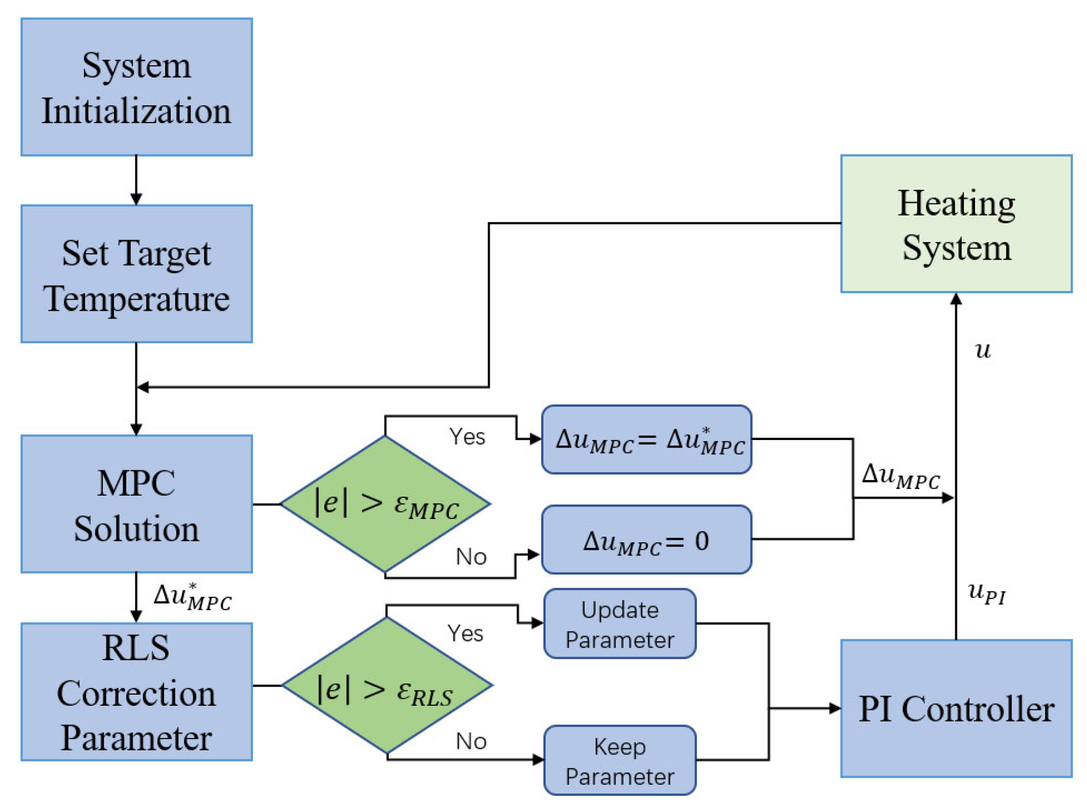
The control architecture developed in this study consists of three layers: a lower-layer PI controller, an upper-layer MPC, and a parameter-adaptive RLS module. These three components are not simply superimposed but are coordinated according to different time scales and functional roles. The overall control procedure is described as follows in Figure 5.

• Initialization: Initialize the model parameters and PI controller parameters, and set the target temperature.
• MPC Optimization: Based on the current system state and reference trajectory, the MPC computes the control increment $\mathrm{∆}{u}_{mpc}$ at the current time step.
• RLS Adaptation: The RLS module uses $\mathrm{∆}{u}_{mpc}$ as the learning signal to estimate the parameter corrections of the PI controller online.
• Parameter and Input Update: The estimated increments $\mathrm{∆}{K}_P$ and $\mathrm{∆}{K}_i$ are applied to the PI parameters with a given weighting factor, and $\mathrm{∆}{u}_{mpc}$ is applied to update the control input $u$.
• Switching Logic and Termination Conditions: The above process is executed iteratively.

• When $\epsilon RLS\le \left|e\left(k\right)\right|\le \epsilon MPC$, the direct action of $\mathrm{∆}{u}_{mpc}$ on the control input is disabled, and MPC only provides the learning signal for the RLS module.
• A smaller error threshold is assigned to RLS than to MPC. When $\left|e\left(k\right)\right|\le \epsilon RLS$, both MPC and RLS are deactivated, and the system gradually enters steady-state operation.

3. Simulation Results and Analysis

Based on the system modeling and control strategy developed in the previous sections, a simulation environment is established on the MATLAB/Simulink R2024a platform to evaluate the dynamic performance of the heating system under representative operating conditions. In practical thermal systems, the large thermal inertia usually results in relatively low measurement noise compared with the dominant system dynamics; therefore, the simulations mainly focus on the deterministic response of the identified model, which already reflects modeling errors and parameter uncertainties to some extent. Step-type disturbances are considered because they represent typical load variations in heating processes, such as sudden changes in heating demand or environmental conditions. Comparative simulations are conducted using several representative temperature control strategies, including conventional PI control, PI–MPC control, fuzzy–PID control, neural-network–PID control, and the proposed PI–RLS–MPC composite control strategy, which are commonly investigated in thermal process control. The comparison aims to demonstrate the performance advantages of the proposed method in terms of tracking capability, steady-state accuracy, disturbance rejection performance, and overall control robustness.

3.1. Simulation Model Setup and Parameter Design

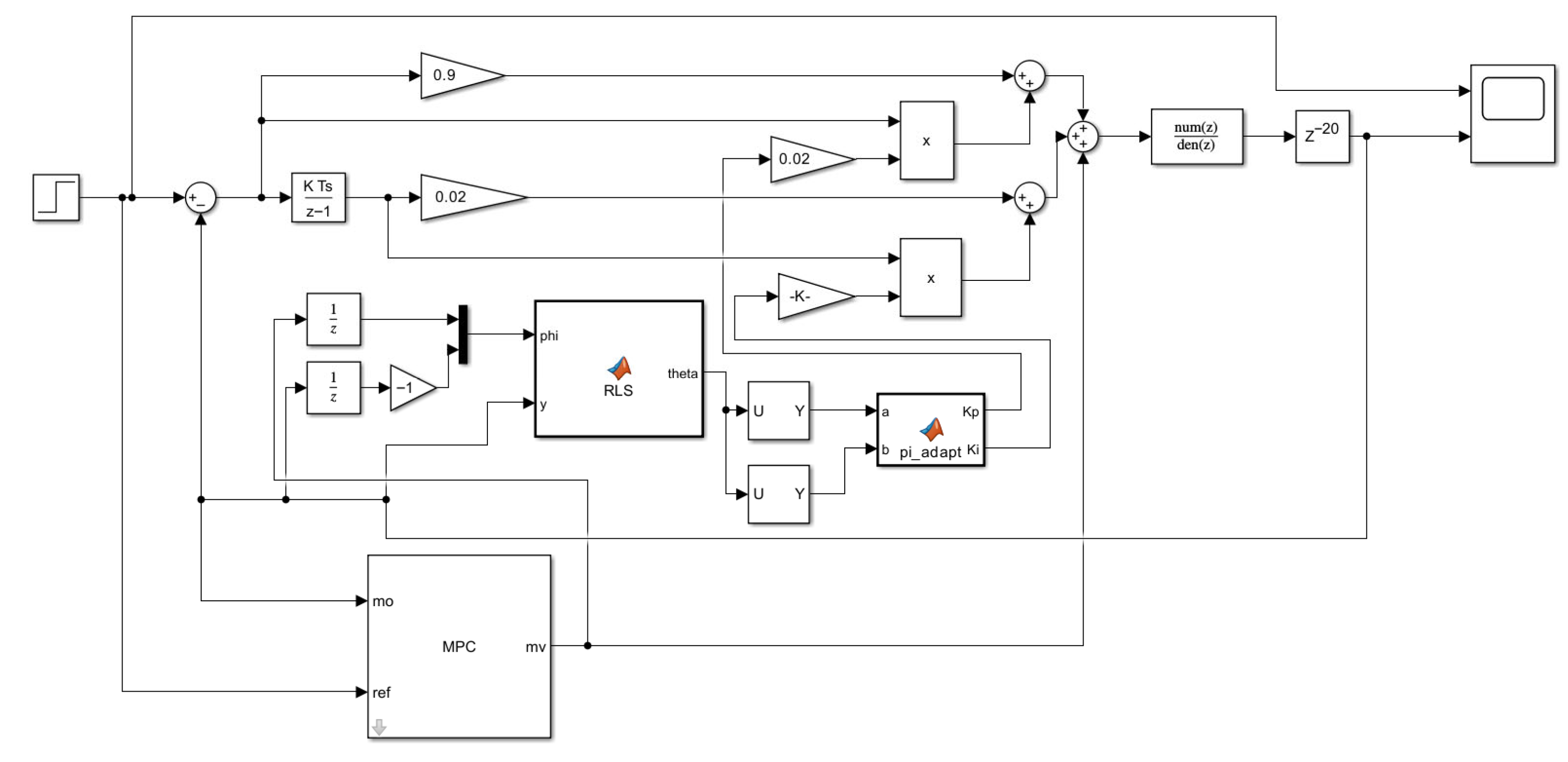
The simulation environment constructed in Simulink according to the proposed control logic is shown in Figure 6.

The controlled plant adopts the model identified in Chapter 2, and the sampling period is set to $T_s$ = 1 s, which is sufficiently small compared with the dominant thermal time constant to ensure accurate discrete-time implementation.

The initial parameters of the PI controller were determined using the tool in MATLAB R2024a based on the identified plant model. The obtained gains were selected as conservative baseline values to ensure stable closed-loop operation before the adaptive mechanism becomes active. Accordingly, the initial parameters of the PI controller are chosen as $K_p$(0) = 0.90 and $K_i$(0) = 0.02. Smaller initial gains would lead to slower responses, whereas excessively large gains may introduce oscillatory behavior during the early transient stage.

The prediction horizon was determined through simulation-based tuning by gradually increasing $N_p$ until further enlargement produced no noticeable improvement in tracking performance. $N_p=40$ is sufficiently long to cover the dominant thermal dynamics of the system while avoiding unnecessary computational burden. A shorter prediction horizon may limit the predictive capability of the controller, whereas an excessively large value increases computational complexity without significant performance improvement.

The control horizon is chosen smaller than the prediction horizon in order to reduce optimization complexity while maintaining sufficient control flexibility. In many thermal control applications, the control horizon is typically selected within one-third to one-fifth of the prediction horizon. A control horizon that is too small may limit the controller’s ability to adjust future control actions, leading to slower dynamic responses. Conversely, an excessively large control horizon increases the optimization dimension and computational burden without providing significant performance improvement. Considering these factors, the control horizon is selected as $N_c=10$ in this study.

The nominal weighting factors in the MPC cost function are selected as $Q_0$ = 1 and $P_0$ = 0.1, which provide a reasonable balance between tracking performance and control effort. These parameters serve as baseline weights used to construct the adaptive weighting matrices $Q\left(k\right)$ and $P\left(k\right)$ defined in Equations (26) and (27). In the MPC optimization problem, $Q\left(k\right)$ penalizes the predicted tracking error while $P\left(k\right)$ penalizes the control increment, thereby determining the trade-off between tracking accuracy and control smoothness. The choice of $Q_0$ = 1 and $P_0$ = 0.1 is motivated by the normalized magnitude of the system output and control input, where a larger $Q_0$ would place excessive emphasis on tracking accuracy and potentially lead to aggressive control actions, whereas a larger $P_0$ would overly penalize control effort and slow down the system response. Therefore, the selected values maintain an appropriate compromise between temperature tracking accuracy and smooth control input variations, which is particularly suitable for thermal systems characterized by large inertia and slow dynamics.

The MPC activation threshold is defined as ${\epsilon }_{MPC}$ = 15% of the reference temperature, allowing the predictive controller to intervene mainly during large deviations. This threshold determines when the MPC layer becomes active to compensate for large tracking errors. If the threshold is chosen too small, for example, close to 5–10%, the MPC controller would be triggered too frequently, which increases computational burden and may lead to unnecessary optimization actions during small disturbances. Conversely, if the threshold is excessively large, such as values above 20%, the predictive controller would intervene too late, reducing the effectiveness of predictive compensation and potentially degrading transient performance. Therefore, ${\epsilon }_{MPC}$ = 15% is adopted as a balanced value that allows MPC to participate mainly during significant deviations while avoiding excessive computational load.

For the RLS module, the learning rate is set to $\alpha$ = 0.02 to ensure gradual and stable parameter adaptation. In this study, the learning rate was selected from a small range of candidate values commonly suitable for slowly varying thermal processes. If $\alpha$ is chosen too small, such as values close to 0.01, the parameter update becomes overly slow, and the adaptive effect on the transient response is weakened. By contrast, if $\alpha$ is increased to a larger value, such as 0.05 or 0.1, the parameter update becomes too aggressive, which may introduce oscillatory parameter variations and deteriorate closed-loop smoothness during the transient stage. Therefore, $\alpha$ = 0.02 was adopted as a compromise value, which provides visible adaptive improvement while still maintaining stable and smooth parameter evolution.

The forgetting factor is chosen as $\lambda$ = 0.99, which allows the estimator to retain sufficient historical information while maintaining the capability to track slow variations in system dynamics. For thermal systems with large inertia, the parameter variation is usually gradual rather than abrupt, and therefore, the forgetting factor should be chosen close to unity. If a smaller value such as 0.98 is used, recent data are weighted too strongly, which improves adaptation speed but may increase estimation fluctuations and make the recursive update more sensitive to measurement noise. On the other hand, if $\lambda$ is selected even closer to unity, such as 0.995, the parameter estimation becomes smoother, but the adaptation to slow model variations becomes weaker. Therefore, $\lambda$ = 0.99 was selected as a balanced value, providing sufficient estimation stability while still preserving the ability to follow gradual thermal dynamic changes.

The RLS activation threshold is defined as ${\epsilon }_{RLS}$ = 5% of the reference temperature, so that parameter adaptation is mainly performed within the moderate error region while unnecessary parameter updates are avoided when the system approaches steady state. This threshold determines when the adaptive parameter update mechanism is activated. If the threshold is chosen too small, such as values close to 1–2%, the adaptation process may be triggered excessively by measurement noise, resulting in frequent parameter updates and increased estimation fluctuations. On the other hand, if the threshold is too large, such as above 8–10%, the adaptive mechanism may not be activated in time, which reduces the effectiveness of online parameter adjustment during transient operation. Therefore, ${\epsilon }_{RLS}$ = 5% is selected as a compromise value that allows parameter adaptation to occur primarily during moderate error conditions while maintaining robustness against measurement noise.

3.2. Qualitative Analysis of Temperature Responses

3.2.1. Step Response Performance

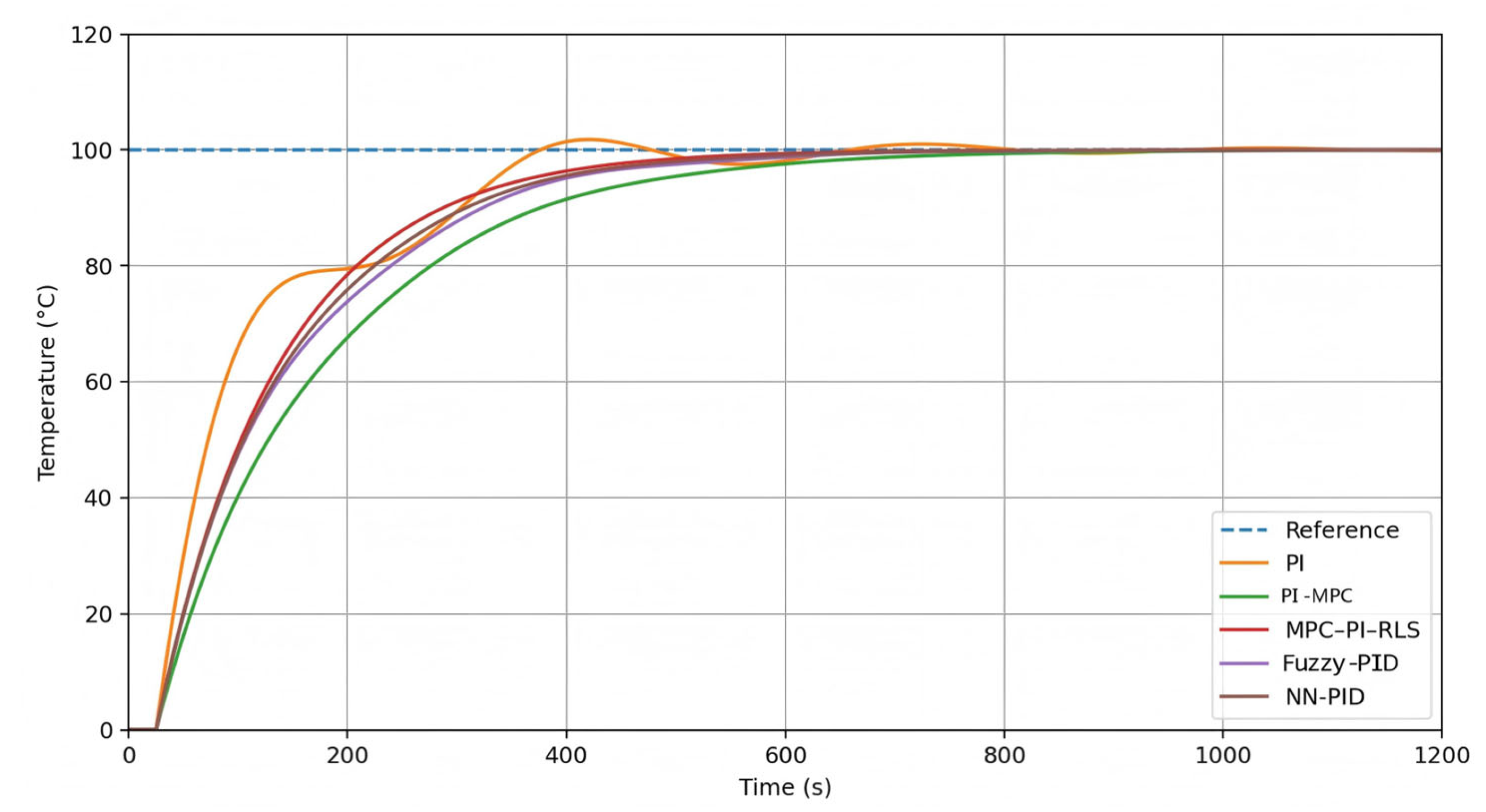
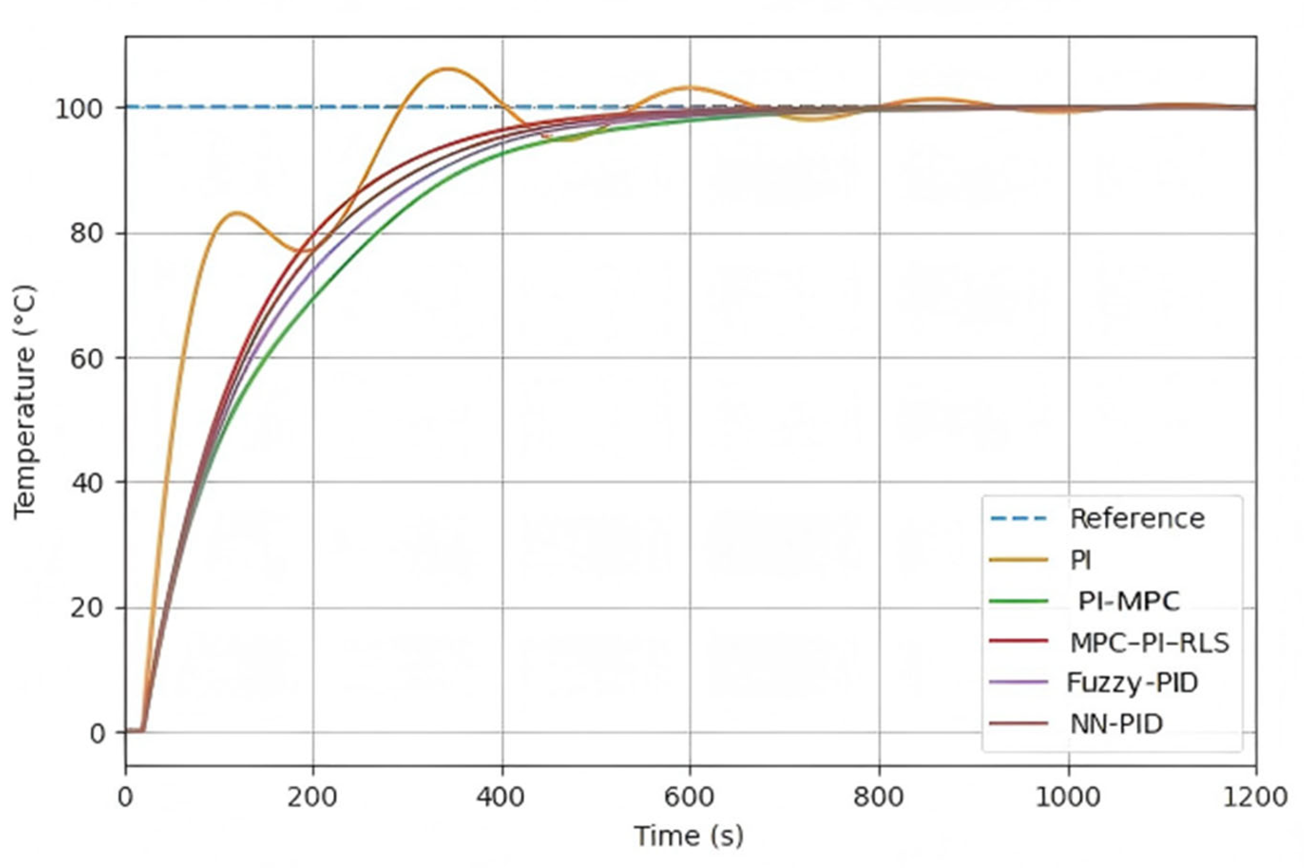
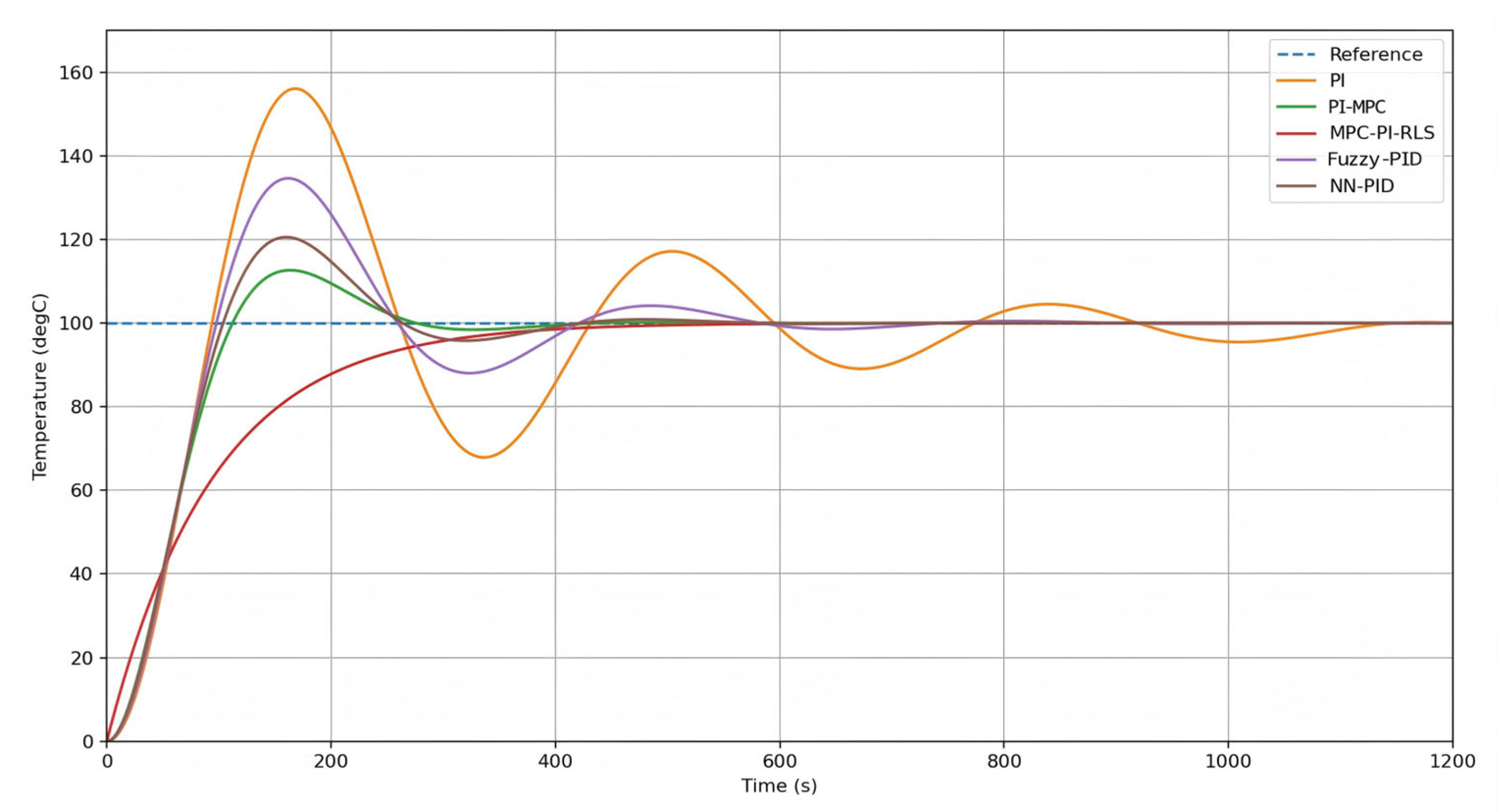
As shown in Figure 7, the reference temperature is set to 100 °C, and the dynamic performances of five control strategies, PI, PI–MPC, PI–RLS–MPC, fuzzy–PID, and neural-network–PID, are compared.

The step responses of the five control strategies over the time interval of 0–1200 s are shown in Figure 7. All controllers are able to drive the system temperature toward the reference value of 100 °C; however, their dynamic performances are significantly different. The conventional PI controller exhibits a faster initial rise but introduces noticeable overshoot and oscillations before settling. The PI–MPC and fuzzy–PID strategies provide smoother responses but with relatively slower convergence to the reference temperature. The NN–PID controller improves the transient performance to some extent. In contrast, the proposed PI–RLS–MPC method achieves a balanced performance, exhibiting a relatively fast rise speed with reduced overshoot and faster convergence to the steady state, demonstrating superior overall control performance.

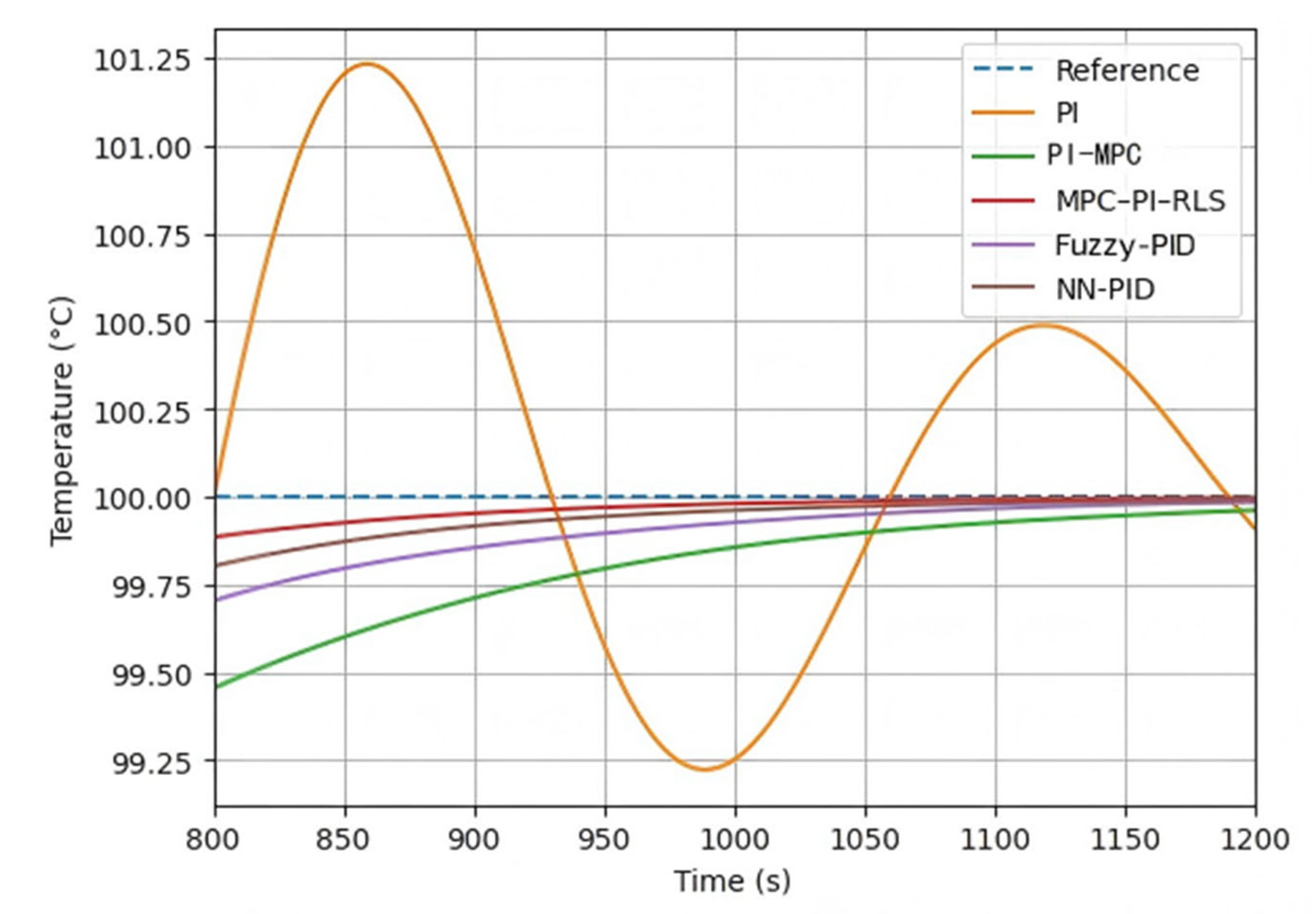
Figure 8 presents the system responses during the late-stage period (800–1200 s), where all control strategies have nearly reached steady-state operation. The conventional PI controller still exhibits slight fluctuations around the reference temperature, indicating a relatively weaker steady-state regulation capability.

By contrast, the other control strategies, including PI–MPC, fuzzy–PID, NN–PID, and PI–RLS–MPC, remain close to the reference temperature with almost no visible oscillations.

Among these methods, the PI–RLS–MPC strategy achieves the most stable steady-state behavior with negligible steady-state error. This result demonstrates that the adaptive adjustment of controller parameters through RLS, together with the predictive optimization of MPC, effectively enhances long-term regulation accuracy and enables the system to maintain a stable temperature after convergence.

3.2.2. Adaptive Parameter Variation Analysis

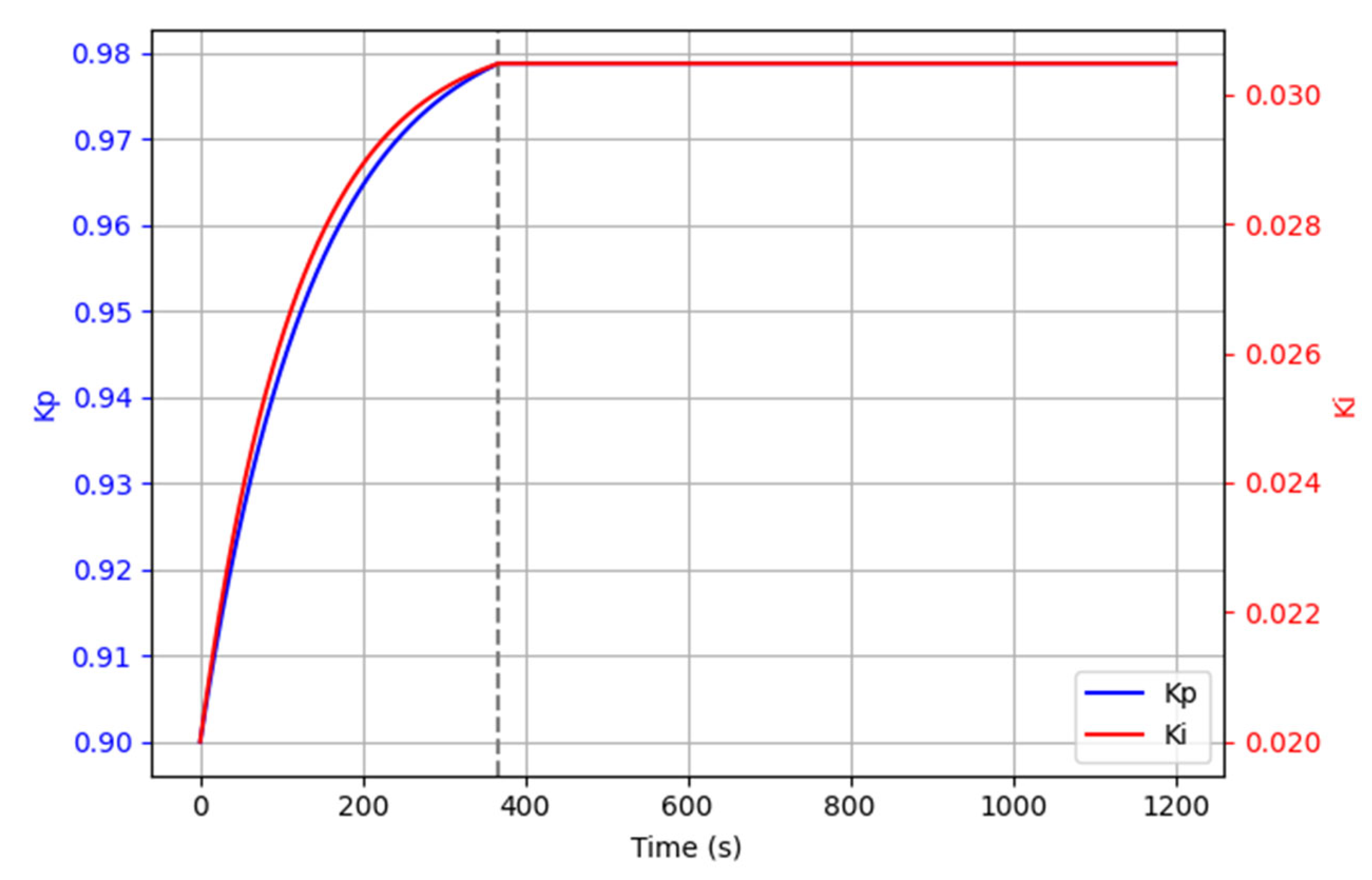
The online variations of $K_p$ and $K_i$ in the PI–RLS–MPC control strategy are shown in Figure 9.

The evolution of the PI controller parameters during the adaptive control process is illustrated in Figure 9. The proportional gain $K_p$ gradually increases from 0.90 to approximately 0.979, while the integral gain $K_i$ increases from 0.020 to about 0.031. Both parameters converge smoothly as the system output approaches the reference temperature. The dashed vertical line indicates the parameter freezing time at 367 s, after which the controller parameters remain constant. This mechanism prevents excessive parameter variations and ensures stable closed-loop control performance.

3.2.3. Disturbance Rejection Performance Analysis

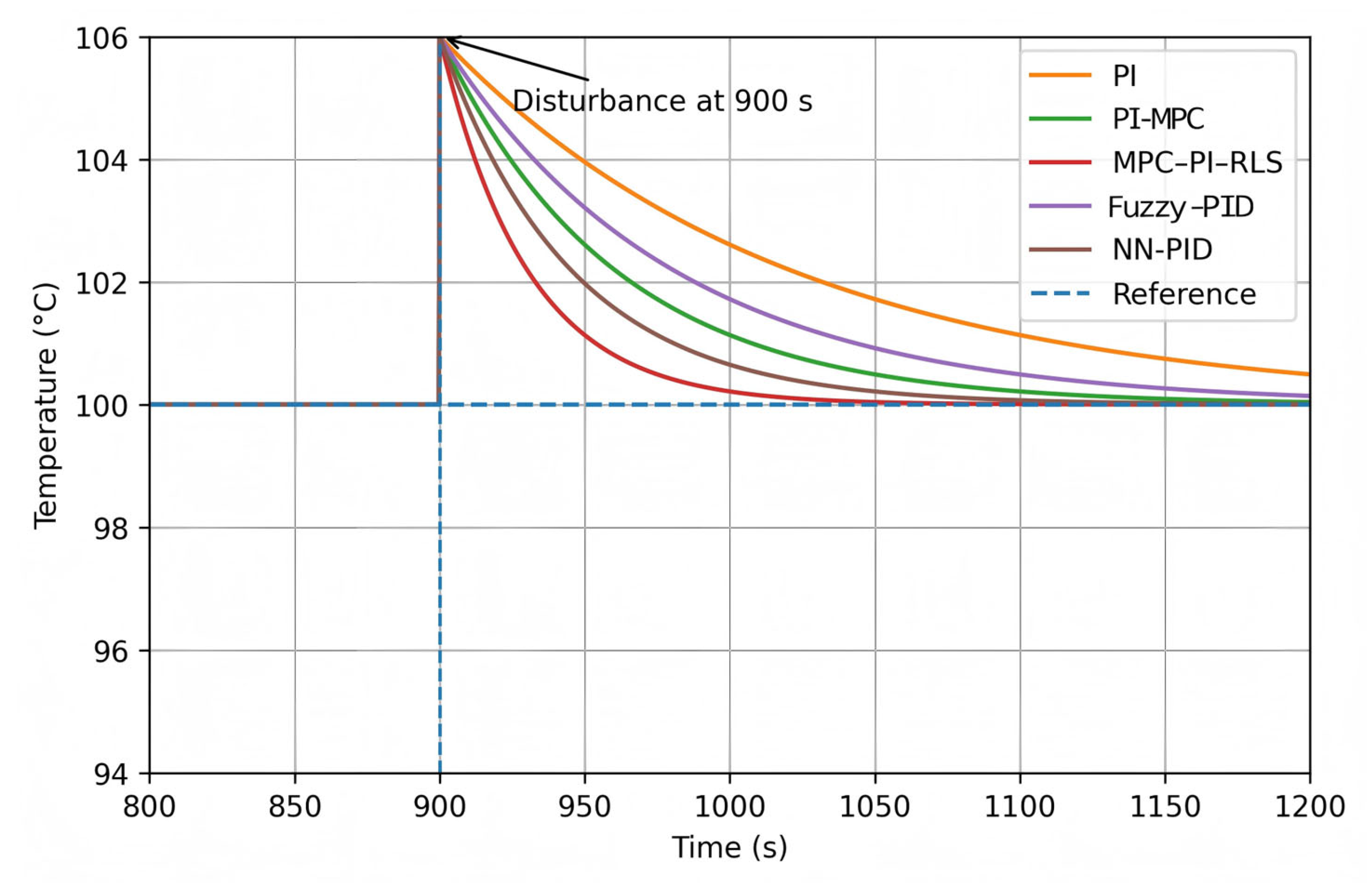
To evaluate the disturbance rejection capability of the proposed PI–RLS–MPC composite control strategy during steady-state operation, a step disturbance is introduced to the system output at t = 900 s after the temperature has stabilized around 100 °C. The temperature response is then locally magnified and analyzed over the interval of 800–1200 s, as shown in Figure 10.

As shown in Figure 10, when the disturbance is introduced at 900 s, the outputs of all control strategies exhibit a temporary deviation from the reference temperature. However, the recovery behaviors of different control methods show noticeable differences.

Under the conventional PI controller, the system demonstrates relatively weak disturbance rejection capability. The disturbance causes a larger temperature deviation, and the recovery process is comparatively slow, indicating that pure feedback control is insufficient to ensure satisfactory disturbance suppression in thermal systems with large inertia.

After introducing MPC, the PI–MPC strategy significantly improves the recovery behavior compared with the conventional PI controller. The temperature deviation is reduced, and the recovery time becomes shorter, showing that predictive optimization helps enhance the disturbance rejection capability.

For comparison, two advanced adaptive control approaches, Fuzzy–PID and NN–PID, are also implemented. Both methods provide better disturbance rejection performance than the traditional PI controller by improving the adaptability of controller parameters.

By contrast, the proposed PI–RLS–MPC composite control strategy exhibits the fastest recovery and the smallest deviation after the disturbance occurs. Through online parameter adaptation using the RLS algorithm combined with predictive optimization of MPC, the controller can rapidly compensate for disturbance effects and drive the system back to the reference temperature. These results demonstrate the superior disturbance rejection capability of the proposed control framework.

3.2.4. Model Mismatch Experiment

To evaluate the robustness of the proposed PI–RLS–MPC strategy under model mismatch, discrepancies are deliberately introduced between the prediction model embedded in the MPC and the actual plant used in simulation. The MPC retains the nominal model identified in Chapter 2 for prediction and optimization, while the simulated plant adopts a perturbed model to emulate modeling uncertainty and operating-condition variations.

Figure 11 shows the step responses when the time delay is increased to 25 s. Under this condition, the differences among the control strategies become more evident. The conventional PI controller exhibits large overshoot and oscillations. The fuzzy–PID and NN–PID controllers improve the damping behavior compared with PI control. By contrast, the proposed PI–RLS–MPC controller achieves a smoother response with faster convergence, indicating superior robustness against time-delay mismatch.

Figure 12 shows the step responses when the inertia parameter $a_2$ is increased by 15% relative to its nominal value. Under this condition, the performance differences among the controllers become more pronounced. The conventional PI controller shows significant oscillations and the slowest convergence. The fuzzy–PID and NN–PID controllers provide improved damping compared with PI control, while the PI–MPC strategy further reduces the oscillation amplitude. By contrast, the proposed PI–RLS–MPC controller achieves the smoothest response and the fastest stabilization, demonstrating superior robustness to inertia parameter variations.

Under both inertia-parameter and time-delay mismatches, the proposed PI–RLS–MPC method maintains smoother responses and improved convergence behavior, suggesting enhanced robustness under different mismatch conditions.

3.2.5. Measurement Noise Robustness Analysis

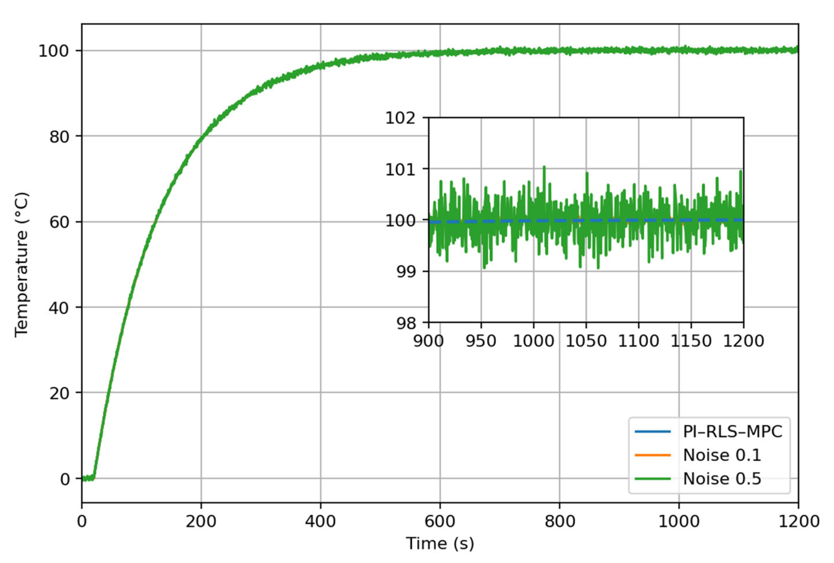
To evaluate the robustness of the proposed control strategy against measurement noise, Gaussian white noise was added to the temperature measurement signal during simulation. Two noise levels with standard deviations of 0.1 °C and 0.5 °C were considered. Since the operating temperature range of the system is approximately 0–100 °C, the corresponding signal-to-noise ratios (SNR) are approximately 60 dB and 46 dB, respectively. The first case represents a typical measurement condition with relatively low sensor noise, while the second case corresponds to a more challenging scenario with stronger measurement disturbances. Both noise levels fall within the typical accuracy range of industrial temperature sensors, allowing the robustness of the proposed PI–RLS–MPC control strategy to be evaluated under realistic measurement conditions.

As shown in Figure 13, the curves are highly overlapping in the steady-state region. To enhance clarity, the PI–RLS–MPC response (blue) is depicted as a dashed line in the inset, while the response under noise level 0.1 is only slightly visible. When measurement noise with a standard deviation of 0.1 °C is introduced, only small fluctuations appear around the response curve, while the overall dynamic behavior remains almost unchanged. Under the stronger noise condition (0.5), the temperature signal shows more noticeable fluctuations; however, the system still maintains stable tracking and converges to the desired temperature.

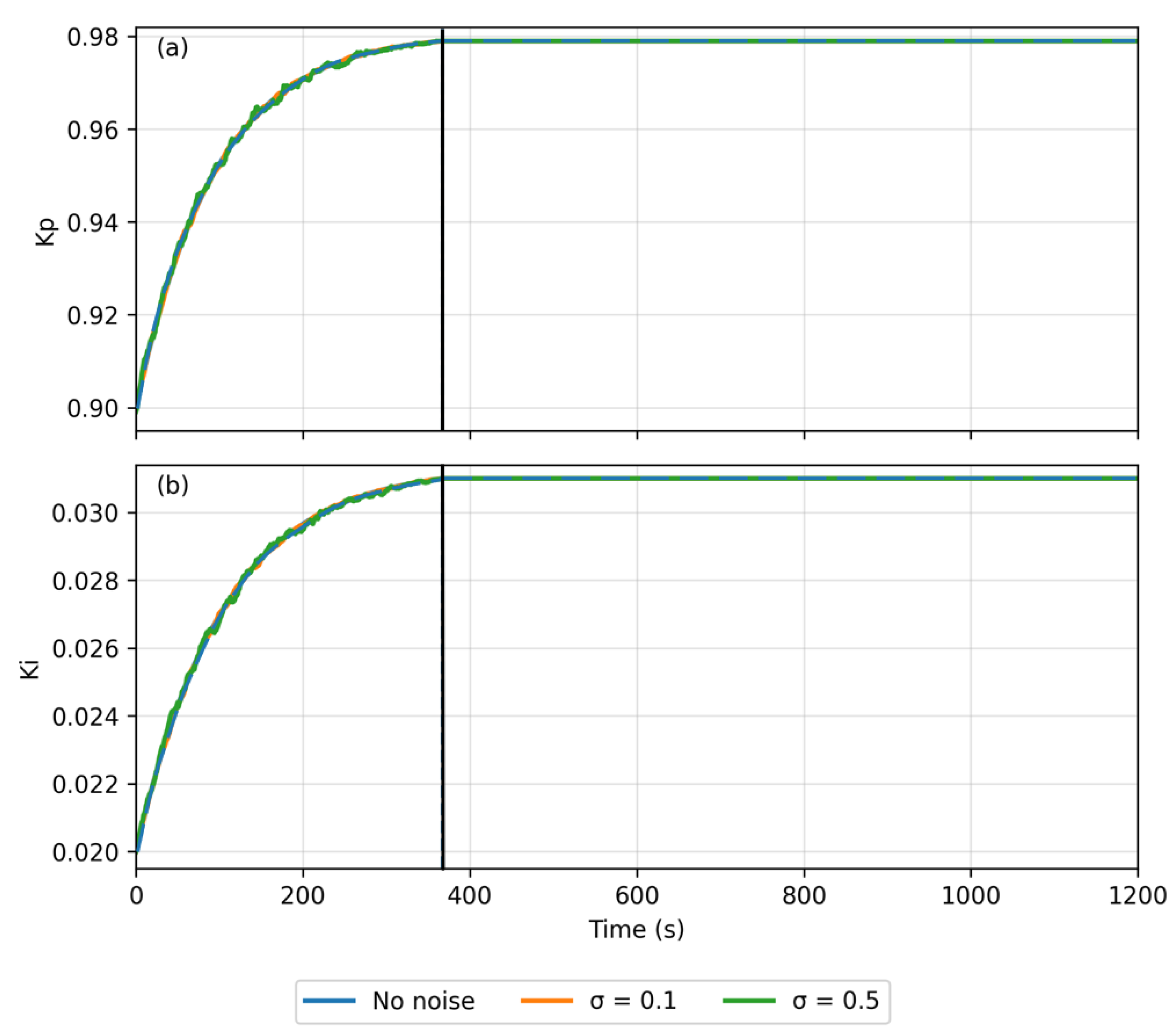
Figure 14 illustrates the evolution of the adaptive PI parameters under different measurement noise levels. It should be noted that the curve corresponding to the noise-free case is plotted as a blue dashed line for clarity, since it is largely overlapped by the curve under $\sigma$ = 0.5 °C. Three cases are considered: the noise-free condition and measurement noise with standard deviations of $\sigma$ = 0.1 °C and $\sigma$ = 0.5 °C. As shown in Figure 14a, the proportional gain $K_p$ gradually increases from its initial value and converges to approximately 0.979 during the transient stage. Figure 14b presents the variation in the integral gain $K_i$, which increases from 0.020 and converges to about 0.031. Although larger measurement noise introduces slightly stronger fluctuations in the parameter trajectories, the overall convergence trend remains consistent with the noise-free case.

3.2.6. Monte Carlo Statistical Robustness Analysis

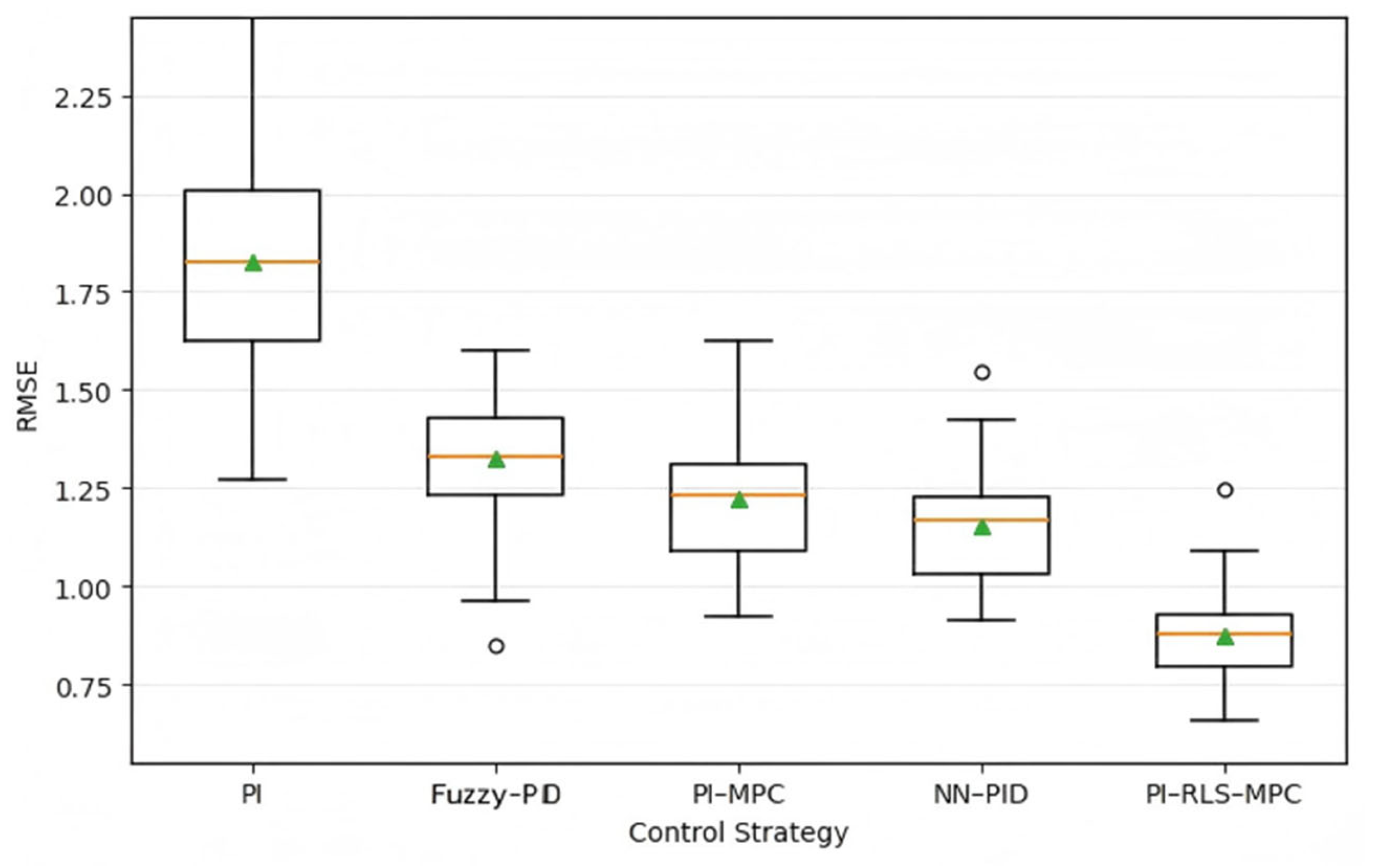
To further evaluate the robustness and reliability of the considered control strategies, Monte Carlo simulations were performed under randomly perturbed operating conditions. In each simulation run, the input delay was randomly varied within 18–22 s, while the inertia-related model parameters were perturbed within ±10% of their nominal values. In addition, Gaussian measurement noise with a standard deviation randomly selected from 0 to 0.5 °C was added to the output signal.

Figure 15 shows the statistical distributions of the tracking RMSE obtained from 100 Monte Carlo simulations for different control strategies, the orange line indicates the median, the green triangles denote the mean values, and the empty bullet represent outliers. In these simulations, key system parameters and disturbance conditions were randomly varied within predefined ranges to evaluate control robustness under uncertain operating conditions. As shown in the Figure 15, the conventional PI controller exhibits the largest RMSE and the widest distribution, indicating relatively poor robustness. The fuzzy–PID, PI–MPC, and NN–PID controllers achieve improved performance, with reduced error levels and narrower distributions. By comparison, the proposed PI–RLS–MPC controller yields the lowest median RMSE and the smallest dispersion, demonstrating better tracking accuracy and more consistent control performance under randomly varying conditions.

3.3. Quantitative Performance Analysis

Table 1. Step response performance comparison of different control strategies.

Control Strategy	Maximum Overshoot (%)	Settling Time (s)	Steady-State Error (°C)
PI	≈6.1	≈484	≈0.18
PI–MPC	≈0	≈466	≈0.05
PI–RLS–MPC	≈0	≈367	≈0.005
Fuzzy-PID	≈0	≈430	≈0.03
NN-PID	≈0	≈400	≈0.008

summarizes the dynamic performance of different control strategies. The conventional PI controller shows the largest overshoot and the slowest convergence. The PI–MPC strategy eliminates overshoot but still exhibits relatively slower settling. The fuzzy–PID and NN–PID controllers improve the dynamic response compared with PI control. In contrast, the proposed PI–RLS–MPC strategy achieves the fastest settling time and the smallest steady-state error, indicating superior control performance.

Table 2. Disturbance rejection performance (step disturbance at t = 900 s).

Control Strategy	Recovery Time (s)	Steady-State Error (°C)
PI	>300	≈0.2
PI–MPC	≈200	≈0.05
PI–RLS–MPC	≈120	≈0.005
Fuzzy-PID	≈240	≈0.02
NN-PID	≈150	≈0.006

summarizes the disturbance rejection performance of different control strategies under a step disturbance applied at $t=900$ s. The recovery time is defined as the time required for the system output to return to the steady-state band after the disturbance occurs. The conventional PI controller exhibits the slowest recovery and the largest steady-state deviation. The fuzzy–PID and NN–PID controllers show improved disturbance rejection compared with PI control. In contrast, the proposed PI–RLS–MPC controller achieves the shortest recovery time and the smallest steady-state error, demonstrating superior disturbance rejection capability.

Table 3. Performance comparison under time-delay mismatch (25 s).

Control Strategy	Maximum Overshoot (%)	Settling Time (s)
PI	≈4.8	≈710
PI–MPC	≈1.1	≈580
PI–RLS–MPC	≈0	≈430
Fuzzy-PID	≈0.9	≈520
NN-PID	≈0.6	≈480

presents the performance comparison under the time-delay mismatch condition (25 s). The conventional PI controller exhibits the largest overshoot and the slowest convergence. The fuzzy–PID and NN–PID controllers provide improved damping compared with PI control. By contrast, the proposed PI–RLS–MPC controller achieves nearly zero overshoot and the fastest settling, indicating stronger robustness to time-delay mismatch.

Table 4. Step-response performance under inertia-parameter mismatch (parameters scaled by 1.15).

Control Strategy	Maximum Overshoot (%)	Settling Time (s)
PI	≈55	≈1100
PI–MPC	≈10	≈380
PI–RLS–MPC	≈0.5	≈410
Fuzzy-PID	≈33	≈640
NN-PID	≈20	≈440

presents the step-response performance when the inertia parameters are increased by 15%. The conventional PI controller exhibits extremely large overshoot and very slow convergence, indicating severe performance degradation. The fuzzy-PID and NN–PID controllers improve the response compared with PI control but still produce noticeable overshoot. The PI–MPC strategy significantly reduces the overshoot and settling time. By contrast, the proposed PI–RLS–MPC controller maintains minimal overshoot and fast stabilization, demonstrating superior robustness to inertia-parameter mismatch.

4. Conclusions

This study proposed a PI–RLS–MPC composite control strategy for a cylindrical thermal performance testing system characterized by large thermal inertia and input time delay. Simulation results demonstrate that the proposed method significantly improves both dynamic and steady-state performance compared with conventional controllers.

Although the proposed PI–RLS–MPC composite control strategy demonstrates promising performance in the presented simulations, the current study is mainly based on numerical simulations of the thermal system. Experimental validation on a real thermal performance testing platform has not yet been conducted. Therefore, future work will focus on implementing the proposed control strategy in practical experiments to further evaluate its real-world performance and applicability. In addition, more extensive experimental studies will be carried out to further verify the effectiveness and robustness of the proposed control framework.

References

1. Crotti, G.; Cantu, R.; Malavasi, S.; Gatti, G.; Laurano, C.; Svelto, C. Wetsuit Thermal Resistivity Measurements. Sensors 2024, 24, 4561. [Google Scholar] [CrossRef] [Scilit] [PubMed]
2. Koenen, A.; Marquis, D.; Dehn, S. Reference Materials for Thermal Conductivity Measurements: European Situation. Buildings 2024, 14, 2795. [Google Scholar] [CrossRef] [Scilit]
3. Lee, J.; Fuji, K.; Hara, K.; Hayasaka, R.; Mechanical, T.O. Simultaneous Measurement of Thermal Conductivity of Insulation Materials in Thickness and In-Plane Directions. Appl. Therm. Eng. 2025, 280, 128004. [Google Scholar] [CrossRef] [Scilit]
4. Fu, J.; Qin, B.; Wu, Y.; He, T.; Zhang, G.; Sun, X. A Control Method of Proton Exchange Membrane Fuel Cell Gas Supply System Based on Fuzzy Neural Network Proportion Integration Differentiation Algorithm. Energy 2025, 315, 134355. [Google Scholar] [CrossRef] [Scilit]
5. Zhao, Z.; Yang, L.; Sun, Q.; Li, F.; Shen, B.; Ye, A. Residual Error Integral Predictor-Based Smith Fuzzy PID Temperature Controller for Thermal Vacuum Test. IEEE Trans. Instrum. Meas. 2024, 73, 9507914. [Google Scholar] [CrossRef] [Scilit]
6. He, F.; Zhao, Y.; Zhao, L.; Wu, X.; Dong, W.; Xie, S.; He, C. Transient Behavior of Fuzzy PID-Controlled Transpiration Cooling with Phase Change Under Dynamic Thermal Environments. Int. J. Therm. Sci. 2025, 217, 110088. [Google Scholar] [CrossRef] [Scilit]
7. Yu, J.; Sun, C.; Zhao, J.; Ma, L.; Zheng, W.; Xie, Q.; Wei, X. Prediction and Control of Greenhouse Temperature: Methods, Applications, and Future Directions. Comput. Electron. Agric. 2025, 237, 110603. [Google Scholar] [CrossRef] [Scilit]
8. Izci, D.; Ekinci, S.; Jabari, M.; Bajaj, M.; Blazek, V.; Prokop, L.; Yildiz, A.R.; Mirjalili, S. A New Intelligent Control Strategy for CSTH Temperature Regulation Based on the Starfish Optimization Algorithm. Sci. Rep. 2025, 15, 12327. [Google Scholar] [CrossRef] [Scilit]
9. Liu, B.; Qian, B.; Liang, Y.; Dai, P.; Li, R.; Wei, Q. Fast and Accurate Auto-Disturbances-Rejection Temperature Control System Based on Particle Swarm Optimized Fuzzy Control: Applied for Particle Three-Dimensional (3D) Printing Prosthetic Orthotic Plate. Addit. Manuf. 2025, 101, 104704. [Google Scholar] [CrossRef] [Scilit]
10. Huang, Y.; Zhang, D.; Zhu, X.; Li, A.; Wang, Y. Genetic Algorithm-Optimized Diode-Based Temperature Control Actuation System. IEEE Access 2025, 13, 52889–52900. [Google Scholar] [CrossRef] [Scilit]
11. Chen, Y.; Jiang, S.; Long, M.; Xu, J.; Liu, Y.; Kong, X.; Wan, Z. Optimization on the Peroxide Ratio Control Strategy of PEMFC System Based on Immune Algorithm. Int. J. Hydrogen Energy 2024, 71, 110–120. [Google Scholar] [CrossRef] [Scilit]
12. Zhang, Z.; Zhou, Y.; Xin, X.; Qian, J.; Liu, Y. A Day-Ahead Operation Regulation Method for Solar Water Heating Based on Model Predictive Control. Energy Build. 2023, 301, 113715. [Google Scholar] [CrossRef] [Scilit]
13. Khan, M.; Tahiyat, M.; Imtiaz, S.; Choudhury, M.A.A.S.; Khan, F. Experimental Evaluation of Control Performance of MPC as a Regulatory Controller. ISA Trans. 2017, 70, 512–520. [Google Scholar] [CrossRef] [Scilit] [PubMed]
14. Sanama, C.; Xia, X.; Nguepnang, M. PID-MPC Implementation on a Chiller-Fan Coil Unit. J. Math. 2022, 2022, 8405361. [Google Scholar] [CrossRef] [Scilit]
15. Chen, D.; Sun, L.; Shen, F.; Gao, G.; Lou, Y.; Dong, G. A Fuzzy Extended PI Observer for State of Charge Estimation of LiFePO4 Batteries Across Broad Temperature Ranges. J. Energy Storage 2025, 128, 116964. [Google Scholar] [CrossRef] [Scilit]
16. Wei, X.; Ye, H.; Wang, G.; Hu, W. Adaptive Thermal Error Prediction for CNC Machine Tool Spindle Using Online Measurement and an Improved Recursive Least Square Algorithm. Case Stud. Therm. Eng. 2024, 56, 104239. [Google Scholar] [CrossRef] [Scilit]
17. Zhao, J.; Shi, L.; Li, J.; Li, H.; Han, Q. A Model Predictive Control Regulation Model for Radiant Air Conditioning System Based on Delay Time. J. Build. Eng. 2022, 62, 105343. [Google Scholar] [CrossRef] [Scilit]
18. Han, X.; Chen, X.; Zheng, F.; Hua, L. An Adaptive PI Control Method Considering Large Inertia for Multi-DoF Forming Robot. IEEE Trans. Instrum. Meas. 2025, 74, 3004712. [Google Scholar] [CrossRef] [Scilit]
19. Lin, L.; Li, F.; Wang, K.; Zhu, L. Composite Estimation: An Asymptotically Weighted Least Squares Approach. Stat. Sin. 2019, 29, 1367–1393. [Google Scholar] [CrossRef] [Scilit]
20. Qian, X.; Huang, K.; Jia, S.; Chen, H.; Yuan, Y.; Zhang, L.; Wang, S. Composition/Temperature Cascade Control for a Kaibel Dividing-Wall Distillation Column by Combining PI Controllers and Model Predictive Control Integrated with Soft Sensor. Comput. Chem. Eng. 2019, 126, 292–303. [Google Scholar] [CrossRef] [Scilit]
21. Tao, J.; Zhu, Y.; Fan, Q. Model Predictive Control for a Class of Systems with Isolated Nonlinearity. ISA Trans. 2014, 53, 1343–1349. [Google Scholar] [CrossRef] [Scilit] [PubMed]
22. Xiang, K.; Song, Y.; Ioannou, P. Nonlinear Auto-Tuning PI Control with Desired Precision Within User-Specifiable Time. IEEE Trans. Cybern. 2025. early access. [Google Scholar] [CrossRef] [Scilit] [PubMed]
23. Sha, X.; Ma, Z.; Sethuvenkatraman, S.; Li, W. Online Learning-Enhanced Data-Driven Model Predictive Control for Optimizing HVAC Energy Consumption, Indoor Air Quality and Thermal Comfort. Appl. Energy 2025, 383, 125341. [Google Scholar] [CrossRef] [Scilit]
24. Ciesielski, M.; Grodzki, G. Heat Transfer in Granular Material: Experimental Measurements and Parameters Identification of Macroscopic Heat Conduction Model. Appl. Sci. 2025, 15, 2596. [Google Scholar] [CrossRef] [Scilit]
25. Sanchez-Calderon, I.; Merillas, B.; Bernardo, V.; Angel Rodriguez-Perez, M. Methodology for Measuring the Thermal Conductivity of Insulating Samples with Small Dimensions by Heat Flow Meter Technique. J. Therm. Anal. Calorim. 2022, 147, 12523–12533. [Google Scholar] [CrossRef] [Scilit]
26. Koller, M.; Unterkofler, J.; Glanz, G.; Lager, D.; Bergmann, A.; Popp, H. Radial Thermal Conductivity Measurements of Cylindrical Lithium-Ion Batteries—An Uncertainty Study of the Pipe Method. Batteries 2022, 8, 16. [Google Scholar] [CrossRef] [Scilit]
27. Mork, M.; Redder, F.; Xhonneux, A.; Müller, D. Real-World Implementation and Evaluation of a Model Predictive Control Framework in an Office Space. J. Build. Eng. 2023, 78, 107619. [Google Scholar] [CrossRef] [Scilit]
28. Sun, H.; Jia, Z.; Zhao, M.; Tian, J.; Liu, D.; Wang, Y. Dynamic Modeling of Heat Exchangers Based on Mechanism and Reinforcement Learning Synergy. Buildings 2024, 14, 833. [Google Scholar] [CrossRef] [Scilit]
29. Gupta, S.; Padhee, S.; Pekar, L. Recursive Least Squares Identification of Heat Exchanger System Using Block-Structured Models. Proc. Inst. Mech. Eng. Part I J. Syst. Control Eng. 2022, 236, 870–879. [Google Scholar] [CrossRef] [Scilit]
30. Zhang, R.; Gao, F. Two-Dimensional Iterative Learning Model Predictive Control for Batch Processes: A New State Space Model Compensation Approach. IEEE Trans. Syst. Man Cybern. Syst. 2021, 51, 833–841. [Google Scholar] [CrossRef] [Scilit]
31. Alsahlani, A.; Ozalp, N. Experimental Performance of a Nonlinear Control Strategy to Regulate Temperature of a High-Temperature Solar Reactor. J. Sol. Energy Eng. 2023, 145, 051011. [Google Scholar] [CrossRef] [Scilit]
32. Reboli, T.; Gini, L.; Mantelli, L.; Traverso, A. Model Predictive Control of a Phase-Change-Material Thermal Energy Storage Device at Industrial Relevant Scale. Energy Convers. Manag. 2025, 346, 120563. [Google Scholar] [CrossRef] [Scilit]
33. Chen, Z.; Qiu, J.; Jin, M. Prediction-Error-Driven Position Estimation Method for Finite-Control-Set Model Predictive Control of Interior Permanent-Magnet Synchronous Motors. IEEE J. Emerg. Sel. Top. Power Electron. 2019, 7, 282–295. [Google Scholar] [CrossRef] [Scilit]
34. Brattley, D.A.; Weaver, W.W. Adaptive PI Control Using Recursive Least Squares for Centrifugal Pump Pipeline Systems. Machines 2025, 13, 1064. [Google Scholar] [CrossRef] [Scilit]
35. Stotsky, A. Recursive Least Squares Estimation with Rank Two Updates. Automatika 2025, 66, 619–624. [Google Scholar] [CrossRef] [Scilit]
Figure 1. The schematic structure of the system.
Applsci 16 02926 g001
Figure 2. Cross-sectional heat transfer structure of the measurement section.
Applsci 16 02926 g002
Figure 3. Comparison between the identified model and experimental data.
Applsci 16 02926 g003
Figure 4. Block diagram of the PI–RLS–MPC control structure.
Applsci 16 02926 g004
Figure 5. Flowchart of the PI–RLS–MPC control procedure.
Applsci 16 02926 g005
Figure 6. Simulation diagram of the PI–RLS–MPC control system.
Applsci 16 02926 g006
Figure 7. Step response comparison of the five control strategies.
Applsci 16 02926 g007
Figure 8. Step response comparison during the steady-state stage (800–1200 s).
Applsci 16 02926 g008
Figure 9. Evolution of the PI controller parameters with parameter freezing.
Applsci 16 02926 g009
Figure 10. Disturbance rejection performance comparison of different control strategies under a step disturbance at 900 s.
Applsci 16 02926 g010
Figure 11. Step response comparison under time-delay mismatch (delay increased to 25 s).
Applsci 16 02926 g011
Figure 12. Step response comparison under inertia mismatch (parameters scaled by 1.15).
Applsci 16 02926 g012
Figure 13. Temperature responses of the PI–RLS–MPC controller under different measurement noise levels, with an inset showing the enlarged steady-state response (900–1200 s).
Applsci 16 02926 g013
Figure 14. Convergence of adaptive PI parameters under different measurement noise levels: (a) proportional gain K p ; (b) integral gain K i .
Applsci 16 02926 g014
Figure 15. RMSE distributions from 100 Monte Carlo simulations for different control strategies.
Applsci 16 02926 g015