Machine Learning for Daylight Performance Prediction

Abstract

Machine learning methods are increasingly applied in daylight performance assessment due to their ability to model complex nonlinear relationships within large datasets while offering substantially faster predictions than conventional simulation workflows. Within this framework, deep learning architectures provide enhanced representational capability for capturing spatial and geometric dependencies. However, existing approaches often lack seamless integration with parametric design environments and offer limited interpretability regarding the influence of design parameters. This paper presents DayANN (Daylight Artificial Neural Network), a feedforward deep neural network developed within a structured Grasshopper-to-machine learning workflow for analyzing daylight performance in a parametrically defined office space. The method employs Climate Studio for Grasshopper to generate 288 simulation scenarios, forming the training dataset for the predictive model. The proposed framework enables automated data transfer, model training, and performance feedback within an iterative design–evaluation loop. In addition to predictive accuracy, SHAP-based interpretability is incorporated to quantify the contribution of individual daylighting parameters. The model achieved high accuracy, with R² values of 0.988 for Useful Daylight Illuminance (UDI) and 0.947 for Daylight Factor (DF), demonstrating that DayANN serves as a computationally efficient, transparent surrogate model suitable for early-stage architectural decision-making.

1. Introduction

The integration of machine learning (ML) and its diverse applications has fundamentally transformed existing approaches to architecture and the built environment. The applications of machine learning algorithms include, but are not limited to, thermal comfort assessment [1,2,3], acoustic performance prediction [4,5], urban representation and digital mapping [6,7], digital reconstruction of architectural heritage, and image classification [8,9,10]. One particularly promising application lies in the realm of daylighting design. While the efficiency of conventional daylight simulation tools in early design has been widely discussed in the scientific literature [11,12,13], machine learning models have recently emerged as a promising alternative, offering competitive prediction accuracy with substantially reduced computational time.

One major drawback of conventional simulations is the considerable effort required to update the simulation model and generate new data, which often limits design flexibility. Expanding the initial model with additional variables complicates the process of updating the corresponding model. This process requires regenerating simulated datasets from scratch using current tools, leading to inefficiencies and wasted resources [14]. These inefficiencies are particularly challenging in dynamic design environments, where rapid feedback and adaptability are essential for exploring diverse design options. Machine learning models present a promising alternative for data-driven decision-making. They are particularly useful in early design stages for evaluating daylight performance, where many aspects are still adjustable, and decisions have a significant impact on the outcomes. Through machine learning, it is possible to extract patterns from data and exploit them to predict outcomes that optimize daylight performance.

One subset of machine learning is deep learning, which uses multi-layer neural networks, often referred to as deep neural networks (DNNs) [15,16,17]. The structure of DNNs is similar to that of artificial neural networks (ANNs), with the primary difference being their greater depth and complexity. The name ‘deep’ itself implies the presence of multiple layers within the network. An ANN, in its simplest form, has an input layer, a hidden layer, and an output layer, whereas a DNN consists of multiple hidden layers connected in complex ways, enabling the network to perform advanced pattern recognition tasks [18,19]. Several architectures allow for specialized construction of deep neural networks. Among them, convolutional neural networks (CNNs), generative adversarial networks (GANs), recurrent neural networks (RNNs), and feedforward neural networks (FNNs) are widely used for various tasks. CNNs have been demonstrated to be effective at recognizing patterns in visual data, while GANs construct generative models through an adversarial process that simultaneously trains the discriminator and generator networks [20]. RNNs are networks with loops that are primarily used to predict sequential data, such as time series, by capturing temporal patterns through their recurrent connections. In contrast, the architecture of FNNs is designed so that each layer progressively transforms the input data into output data in a single forward direction without any recurrence. Each subsequent layer builds on the features extracted by previous layers to further refine and optimize the final predictions [21,22].

In the realm of daylight assessment, there is considerable evidence supporting the use of deep learning, including its ability to model nonlinear relationships in large datasets and its potential to achieve high predictive accuracy. This capability enables a faster evaluation of daylighting potential, and hence, design professionals rely more than ever on deep learning algorithms. However, one limitation of the multi-layer nonlinear structure in deep neural network models is that they are characterized as black boxes. Black-box models are those in which the internal mechanisms and decision-making processes are not easily interpretable [23]. What this means is that it is difficult to determine which specific input features had the greatest influence on daylight prediction. Further challenges beyond interpretability include issues associated with generalization. Given that neural networks rely on the training data, the prediction of daylight performance and the accurate estimation of how specific input features influence output (i.e., daylight performance metrics) are inherently limited by the diversity and quality of the data provided. On the other hand, training a model to minimize loss can sometimes lead to overfitting, where the model becomes overly focused on the noise in the data instead of capturing the underlying patterns. This reduces the ability of the network to generalize to unseen data. Generalization concerns can be addressed through the application of regularization methods and effective data pre-processing [24].

The present study formulates a machine learning model to predict daylight performance in office spaces with varying window configurations and geometric layouts. While numerous studies have applied artificial neural networks to daylight prediction, the contribution of this work lies primarily in the establishment of a structured and automated Grasshopper-to-machine learning workflow that enables seamless integration between parametric modeling and predictive analysis. This integration supports an iterative design–evaluation loop with significantly reduced computational overhead compared to repeated simulation-based assessments. In addition to predictive performance, the study addresses the “black box” limitation commonly associated with deep neural networks. Black-box models are often criticized for their lack of transparency, as designers cannot readily determine how specific geometric parameters influence predicted daylight metrics. To overcome this limitation, SHAP-based interpretability is incorporated to quantify the contributions and interactions of input variables, thereby improving the transparency and practical usability of the model. The predictive framework, referred to as DayANN (Daylight Artificial Neural Network), employs a feedforward neural network trained with backpropagation, and its methodological assumptions and evaluation strategy are detailed in the following sections.

2. Literature Review

The inherent challenges and opportunities associated with the application of deep neural networks in daylight prediction are well established in the literature. Ayoub [25] provided a comprehensive summary of existing studies that employed machine learning algorithms, comparing them based on a set of criteria, including the scope of prediction, the algorithms used, the data sources, and predictive performance. The author discussed how machine learning models could serve as alternatives to traditional daylight simulation methods, emphasizing their potential in current and emerging applications. The research demonstrates that the machine learning models used are diverse in their approaches and capabilities. Fast computation times and accurate predictions with lower error rates were cited as advantages of machine learning approaches over conventional daylight performance simulations. Ngarambe et al. [26] carried out a review that builds on the framework established by Ayoub [25], discussing studies that use machine learning to optimize daylighting performance at both the conceptual design stage and the operational phase for daylight control. The authors categorized the studies according to the sources of model training data, climate conditions, input and output variables, and the algorithms employed. The review found that artificial neural networks trained with supervised learning were the most applied machine learning algorithms. Additional focus was given to the implications and challenges of relying on machine learning models with limited generalization and scalability, as well as the progress made in addressing these issues through the integration of transfer learning and incremental learning techniques.

One recent study by Keskin [27] raises concerns about the integration of artificial neural networks on larger scales. The review revealed that many ANN-based approaches do not account for elements typically present in a real-world setting, such as surrounding buildings and obstacles, which are crucial for accurate predictions. The use of neural networks in urban daylight assessments remains relatively unexplored but holds promising potential for future research. Numerous studies have employed machine learning algorithms for daylight prediction and optimization in buildings.

Table 1. Summary of the studies using machine learning algorithms to predict daylight performance metrics. Note that ANN refers to deep neural network-based ANNs as reported in the studies.

Study	Test Space	Location	Method	Input Variables	Output Variables	Model Performance Metrics
Mashaly et al. [28]	A generic office space	100 different cities	ANN cGAN	Room depth, room width, orientation, latitude, clearness index, window-to-wall ratio	SDA and ASE	MAE = 1.7–4.5% RMSE = 3.0–7.4% R2 = 0.90–0.99
Dieguez et al. [29]	Residential spaces	Stockholm, Sweden	ANN XGBoost cGAN	Room geometry, window geometry and position, obstruction features	Daylight Factor	MSE = 0.0003–0.098% MAE = 0.0016–0.0054%
Luo et al. [30]	Teaching building clusters	China	ANN CNN XGBoost	Spatial layout features including orientation and the distance between buildings	sDA and ASE	MSE = 0.31–0.66% R2 = 0.85–0.95
Kat et al. [31]	Apartment buildings	Switzerland		Room geometry and orientation, window placement, and surrounding environmental features	Illuminance and view metrics	MSE = 0.04–0.05% R2 = 0.74–0.78
Liu et al. [32]	A generic four-story terraced school building	Guangzhou, China	ANN	Spatial geometric parameters of skylight and sidelight	sDA, ASE, Uniformity of Daylight Factor	MAE = 0.03–2.32% RMSE = 0.04–3.68% R2 = 0.74–0.78
Wang et al. [33]	12 high-rise residential buildings	Beijing, China	ANN	Spatial position variables: X-axis, Y-axis, and Z-axis	DF, Sky view ratio, Window sunlight hours, Site sunlight hours, Universal thermal climate index	Correlation coefficient (R) = 0.21–0.86
Kristiansen et al. [34]	A generic residential space	Norway	ANN	Zone variables (glass properties, window geometry, and orientation) and sensor-node variables based on different WWR variations	Annual hourly illuminance, operative temperature	RMSE = 78–79% PCC = 10–21%
Le-Thanh et al. [35]	Generic medium-sized buildings	Vietnam	ANN	Relative positions of sensors, in relation to windows and surrounding obstacles	UDI	R2 = 0.78–0.89 MAE = 4.12–6.12% RMSE = 8.09–11.49%
Nourkojouri et al. [36]	A side-lit shoebox model	Tehran, Iran	ANN	Window sill height, window height, and window divisions	UDI, sDA, mDA, ASE, sVD	MAE = 0.02–0.06% MSE = 0.0008–0.007%
Lin and Tsay [37]	A generic office space	Taipei, Taiwan	ANN	Intermediary features: Sensor point position, shading, sunlight hours	sDA, ASE	R2 = 0.81–0.91 RMSE = 6.09–8.98%
Ngarambe et al. [26]	A generic space	Not Reported	RF DNN GLM GBM	Three building factors, seven climatic factors, and time	Illuminance	R2 = 0.95–0.99 RMSE = 1.99–4.77% MAE = 0.69–2.24
Lorenz et al. [38]	A school building	Germany	ANN	Atrium geometry and orientation	sDA	MAE = 0.66–6.23% MSE = 0.0005–0.0009% RMSE = 1.12–11%
Lorenz and Jabi [39]	A generic office space	Not Reported	ANN	Room and window dimensions, orientation, number of windows, and average distance to windows	DA	MSE = 0.11–0.28%
Ahmad et al. [40]	A classroom	UK	RF ANN	solar altitude angle, solar azimuth angle, direct normal radiation, diffuse horizontal radiation	Energy consumption and hourly illuminance values	R2 = 0.98–0.99
Zhou and Liu [41]	A generic office building	Virginia, USA	SVM, ANN, PCA	Glazing transmittance, blind reflectance, and weather condition	UDI, energy consumption	R2 = 0.92–0.96

summarizes relevant work, much of which has been conducted in the past decade.

There is considerable research on the interfaces between daylight performance simulation and machine learning, covering a range of applications, including predictive modeling, optimization, and performance analysis, as illustrated in Table 1. Mashaly et al. [28] developed the Daylighting Performance Prediction Tool (DPPT), a web-based interface designed for rapid assessment during early design stages. By training an ANN on a dataset of 367,254 simulations across 100 cities, the authors were able to predict spatial Daylight Autonomy (sDA) and Annual Sunlight Exposure (ASE) with near-instantaneous feedback. The integration of the clearness index and latitude as primary predictors enabled the tool to generalize daylighting performance across 3000 global locations. The model yielded high predictive accuracy, with MAE values consistently remaining below the 5% threshold across most latitudes. While the highest accuracy was observed at lower latitudes due to stable solar conditions, performance slightly declined at higher latitudes, where daylighting conditions exhibit greater variability.

One study by Liu et al. [32] developed an ANN-based model specifically designed for a four-story terraced school building, aimed at investigating daylighting strategies in educational settings. The model incorporated geometric parameters of skylight and sidelight configurations, with room depth and room width being crucial parameters for improving the model’s adaptability. The model achieved R² values ranging from 0.75 to 0.87, leading the authors to conclude that the model demonstrated notable generalization capabilities and had the potential to replace conventional daylighting simulation methods. In another study by Wang et al. [33], a sensitivity analysis was performed to investigate how different factors influenced the performance of an ANN model. The factors evaluated included the size of the training sample, the number of hidden layer neurons, and the normalization method. Examination of the results reported in the study provides support for an effect of the factors examined, except for the normalization method, which had little or no effect. Larger training sample sizes yielded more accurate predictions, and the model achieved its best training performance when the number of hidden layer neurons was 1.5 times that of the input layer.

In a study by Lorenz and Jabi [39], the impact of input parameters was analyzed when using an ANN model to predict daylight autonomy levels in a typical office building layout. As the authors suggest, increasing the amount of training data generally improves the accuracy of the model. A more recent study by Lorenz et al. [38] employed a parametric model as a benchmark for an ANN-based prediction of spatial daylight autonomy. By analyzing a school building with a central atrium, the study demonstrates a workflow for integrating the ANN model with daylight performance simulations. The design variables considered in the study included atrium geometry and orientation, resulting in 54 potential design solutions. The proposed model achieved strong predictive performance across varying design scenarios. Le-Thanh et al. [35] examined the relationship between building layout and the position of sensor points in applying a machine learning model to predict UDI across four ranges (UDI-fell-short, UDI-supplementary, UDI-autonomous, and UDI-exceeded). Inputs to the model included the relative positions of sensors, taking into account their proximity to windows and surrounding obstacles. A dataset of 400 layout variations was used to train the ANN model. The highest accuracy was observed in predicting UDI-e and UDI-a, with R² values of 0.995 and 0.975, respectively. UDI-s and UDI-f demonstrated lower accuracy, with R² values of 0.898 and 0.890, respectively. Another study by Lin and Tsay [37] developed an ANN-based model to assess the impact of facade design on daylight performance and demonstrated its application in an office space with various facade configurations. The ANN model was trained on intermediary data generated through a pre-processing approach. The model achieved an accuracy range of 0.85 to 0.91 in predicting facade performance.

An example of how well different machine learning algorithms perform in predicting the distribution of indoor daylight illuminances is highlighted by Ngarambe et al. [26]. To identify the best-performing algorithm, the authors trained a series of iteratively reweighted generalized linear models (GLMs), DNNs, random forests (RFs), and gradient boosting models (GBMs). This approach goes beyond evaluating a single machine learning model, providing a comparative analysis of multiple models to identify which performs better. According to the reported results, DNNs achieved the highest performance among all algorithms, with an R² value of 0.99. Further evidence is provided by Ahmad et al. [40], who compared the performance of ANNs and RFs using daylight illuminance and energy consumption datasets. RF showed slightly better performance than ANNs in predicting daylight illuminance, while ANNs outperformed RF in energy consumption predictions.

Alongside daylight prediction, machine learning algorithms have been integrated into energy prediction and view quality assessments. One study by Nourkojouri et al. [36] has investigated the ability of ANNs to predict a variety of metrics, including UDI, Spatial Daylight Autonomy (sDA), Annual Sunlight Exposure (ASE), and view metrics. High predictive accuracy was achieved by integrating features, such as dimensions, interior surface reflectance, shading states, window height, sill height, and orientation, into the model. In another study, Zhou and Liu [41] compared three algorithms to predict UDI and energy consumption in a generic office building. The three algorithms were Principal Component Analysis (PCA), ANN, and Support Vector Machine (SVM). They found that the neural network, when combined with PCA, outperformed the other algorithms in terms of accuracy. As part of a multi-objective optimization study on daylight availability, thermal comfort, and energy performance, Kristiansen et al. [34] investigated the capability of ANNs to predict annual daylight illuminance and operative temperature within a generative residential space designed in a parametric environment. The authors defined two sets of input variables: zone variables and sensor-node variables. Window geometry and properties formed the basis of the zone variables, while sensor-node variables depended on window-to-wall ratio (WWR) variations, including vertical and horizontal views as well as view direction, measured in degrees. The results revealed variations in the predictive performance of ANNs, with higher accuracy achieved for operative temperature and lower accuracy for daylight illuminance. One possible reason for this difference, as reported by the authors, is that the prediction of operative temperature relies on relatively stable parameters, whereas daylight illumination is influenced by more dynamic and complex factors, making it more challenging for ANNs to predict accurately.

Most studies tended to use numerical input data from a single modality, except for one study by Kat et al. [31], which used an image-based model incorporating multimodal data to predict daylight provision and view quality in residential building layouts. The best-performing model achieved mean squared errors (MSEs) of 0.04 and 0.05 and R² values of 0.74 and 0.78 for daylight and view metrics, respectively. Dieguez et al. [29] further performed a comparative analysis of numerical regression and image-based encoding via a pix2pix framework for daylight factor prediction. Based on a large-scale surrogate dataset derived from residential design scenarios in Stockholm, the authors evaluated the performance of two numerical models (ANN and XGBoost) against an image-based conditional GAN (cGAN). The findings indicated that, while both approaches achieve high predictive accuracy, they present distinct trade-offs regarding model interpretability, data intensity, and seamless integration into architectural design workflows. In another study examining deep learning algorithms for predicting the daylighting performance of teaching building cluster layouts, Luo et al. [30] found that their model, utilizing an autoencoder for feature extraction, achieved high accuracy in predicting sDA and ASE. The model demonstrated R² values of 0.95 and 0.85 for sDA and ASE, respectively, with MSE values of 0.31 and 0.66.

The studies reviewed in this section are distinguished based on the context of application of machine learning algorithms. The samples included a range of spaces and functions, such as offices, classrooms, and residential spaces. A common finding across the studies reviewed is that machine learning models demonstrate significant potential to accurately predict daylighting performance. The usual approach, as adopted by most of the studies in Table 1, is to evaluate performance based on overall accuracy, measured by metrics such as root mean squared error (RMSE), mean absolute error (MAE), and MSE. According to the studies, the models consistently achieved high predictive accuracy, with R² values frequently exceeding 0.8, indicating a strong correlation between predicted and actual values. Additionally, error metrics remained within acceptable ranges, demonstrating the reliability and robustness of these approaches across various contexts. Despite the promising performance reported in these studies, several limitations remain evident in the existing literature. First, many approaches focus primarily on predictive accuracy without integrating machine learning models into iterative parametric design workflows. Second, interpretability is often treated superficially or omitted entirely, limiting the ability of designers to understand how geometric variables influence predicted daylight metrics. Third, most studies evaluate models within narrowly defined geometric scenarios without explicitly discussing generalization boundaries or computational efficiency relative to repeated simulation. These gaps indicate a need for a framework that not only achieves high predictive performance but also supports transparent parameter sensitivity analysis and seamless integration into early-stage architectural design. The present study aims to address these limitations by combining workflow automation with SHAP-based interpretability within a structured machine learning framework.

3. Methodology

3.1. Modeling Framework

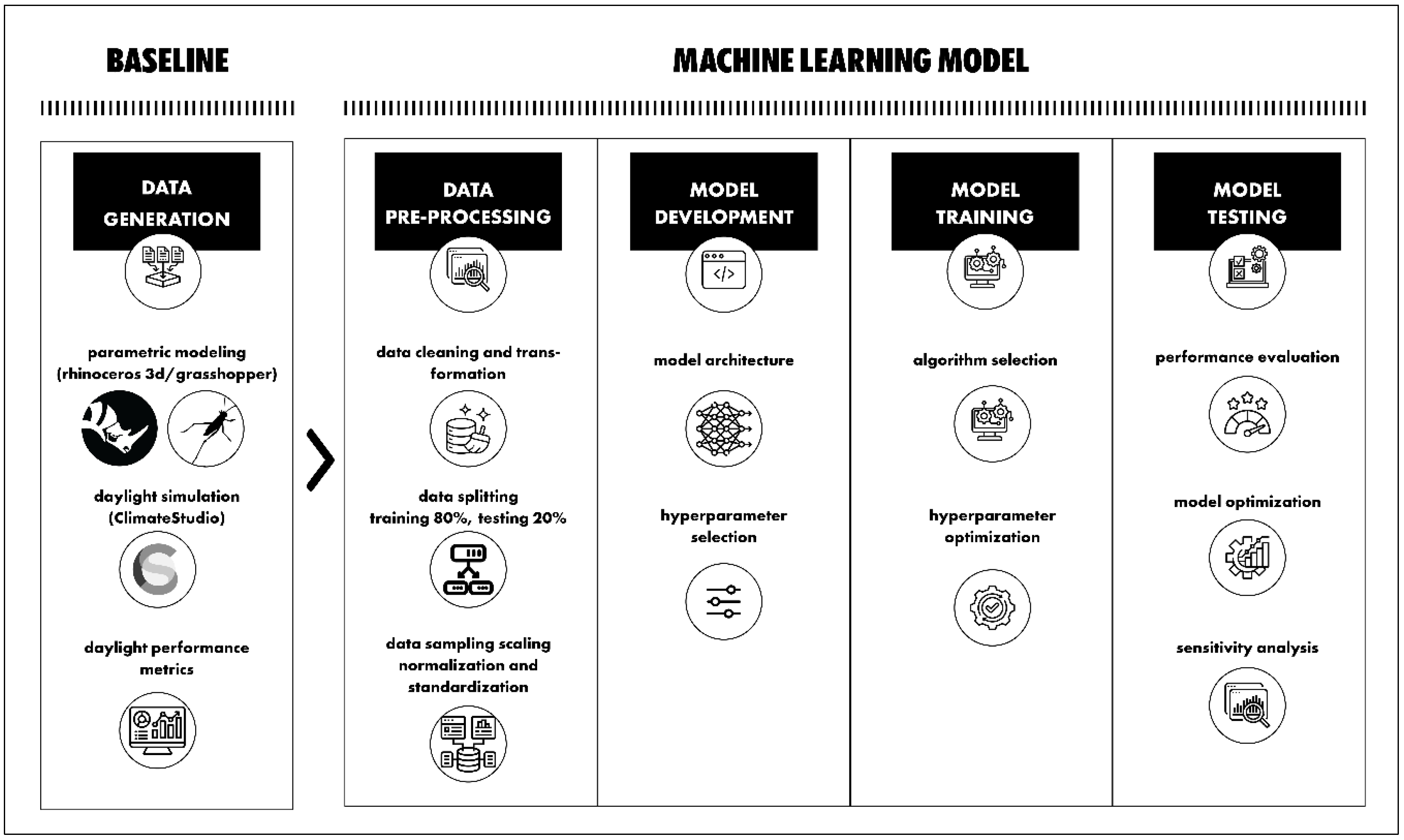
The framework is based on identifying optimal parameters for daylight performance through machine learning, following the approach used in previous research. The proposed model employs supervised machine learning, trained on a simulation dataset, to predict daylight performance metrics for input parameters within the bounds of the training range. An overview of the process underlying the model development is given in Figure 1.

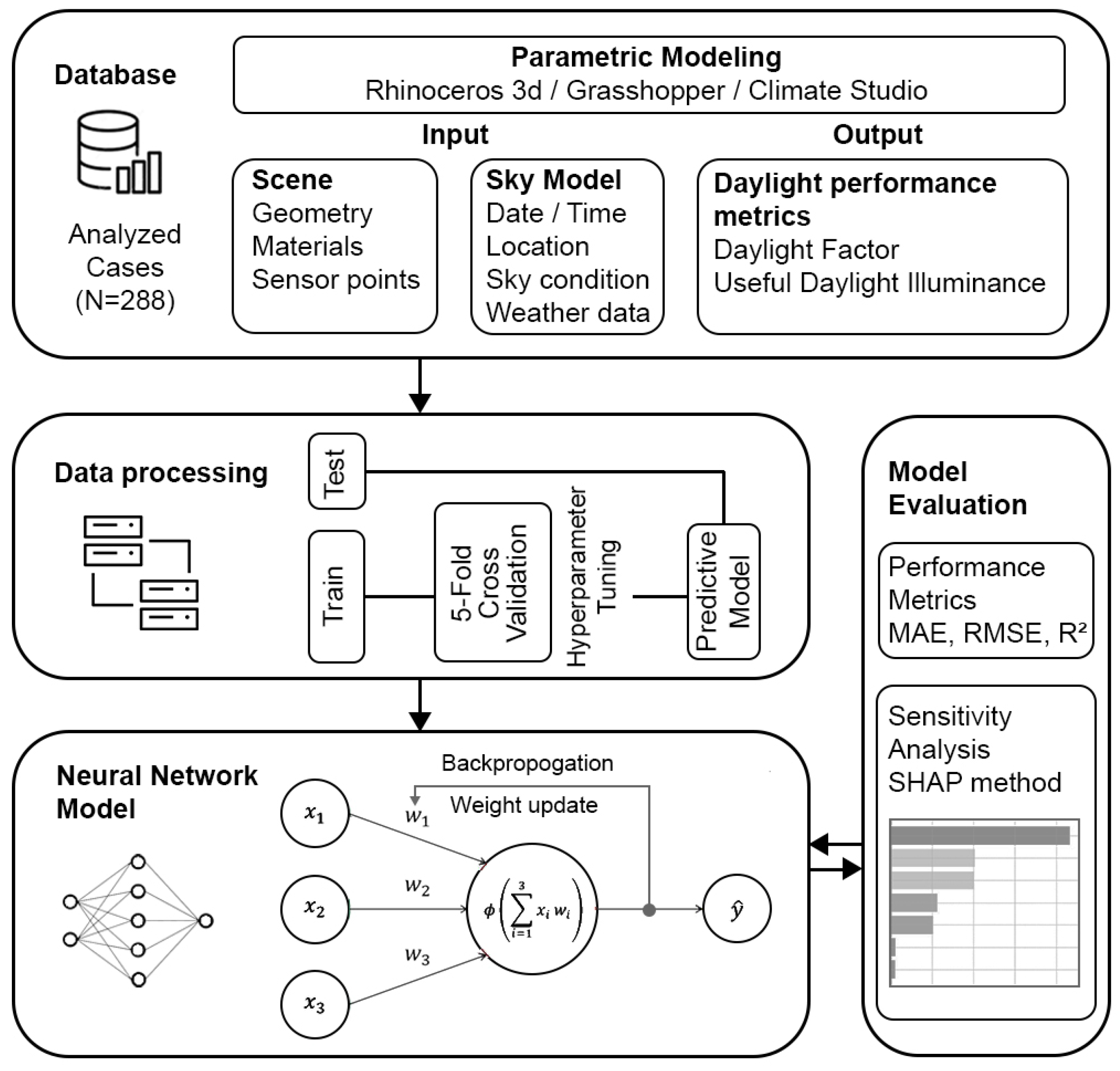
As illustrated in Figure 1, the workflow consists of several interrelated phases. The first phase involves developing a simulation model within a parametric design environment. For this purpose, a parametric modeling workflow was implemented in Grasshopper, an algorithmic modeling plugin integrated into Rhino 3D. Then, daylight performance metrics were calculated in Radiance via Climate Studio (CS), with a 0.5 m sensor grid resolution, 5 ambient bounces, and the EnergyPlus weather data file for Istanbul, Turkey. The LunchBox plugin for Grasshopper was utilized to enable data transfer between the parametric design workflow and Microsoft Excel. This process was followed by a pre-processing phase, during which the dataset generated by the simulation model was normalized and converted into a format for machine learning algorithms to analyze and learn from. Specifically, the raw simulation data was transformed into features to be used as inputs for machine learning algorithms. To ensure robust and generalizable model performance, the pre-processed dataset was evaluated using 5-fold cross-validation, in which the data were divided into five equal subsets, with each subset serving once as the test set and the remaining subsets used for training. Within each training portion, a validation subset was defined to monitor convergence and implement early stopping. This hierarchical splitting strategy ensured that model tuning was performed without exposure to the test data, thereby preventing information leakage and providing an unbiased estimate of predictive performance. The hyperparameters were defined prior to training based on preliminary experimentation and remained fixed during cross-validation. Model performance was assessed on the held-out test fold in each iteration. The numerical output from the machine learning model was streamed back into Grasshopper for visualization, and predictive accuracy was evaluated using standard performance metrics and compared with the corresponding simulation results. The methodological framework of the study is depicted in Figure 2, with the pseudocode of the computational workflow presented in the Supplementary Materials (Algorithm S1).

A side-lit office room is selected as the case study environment due to its practical and research relevance in daylight performance assessment. Office spaces are characterized by regular occupancy patterns, standardized working hours, and strong dependence on perimeter daylight zones, making them a common benchmark in daylighting research and building performance guidelines. Their relatively controlled geometric typology allows systematic parametric variation while maintaining comparability with the existing literature. Although the proposed machine learning framework is not limited to office environments, this typology provides a consistent and widely studied reference condition for methodological validation.

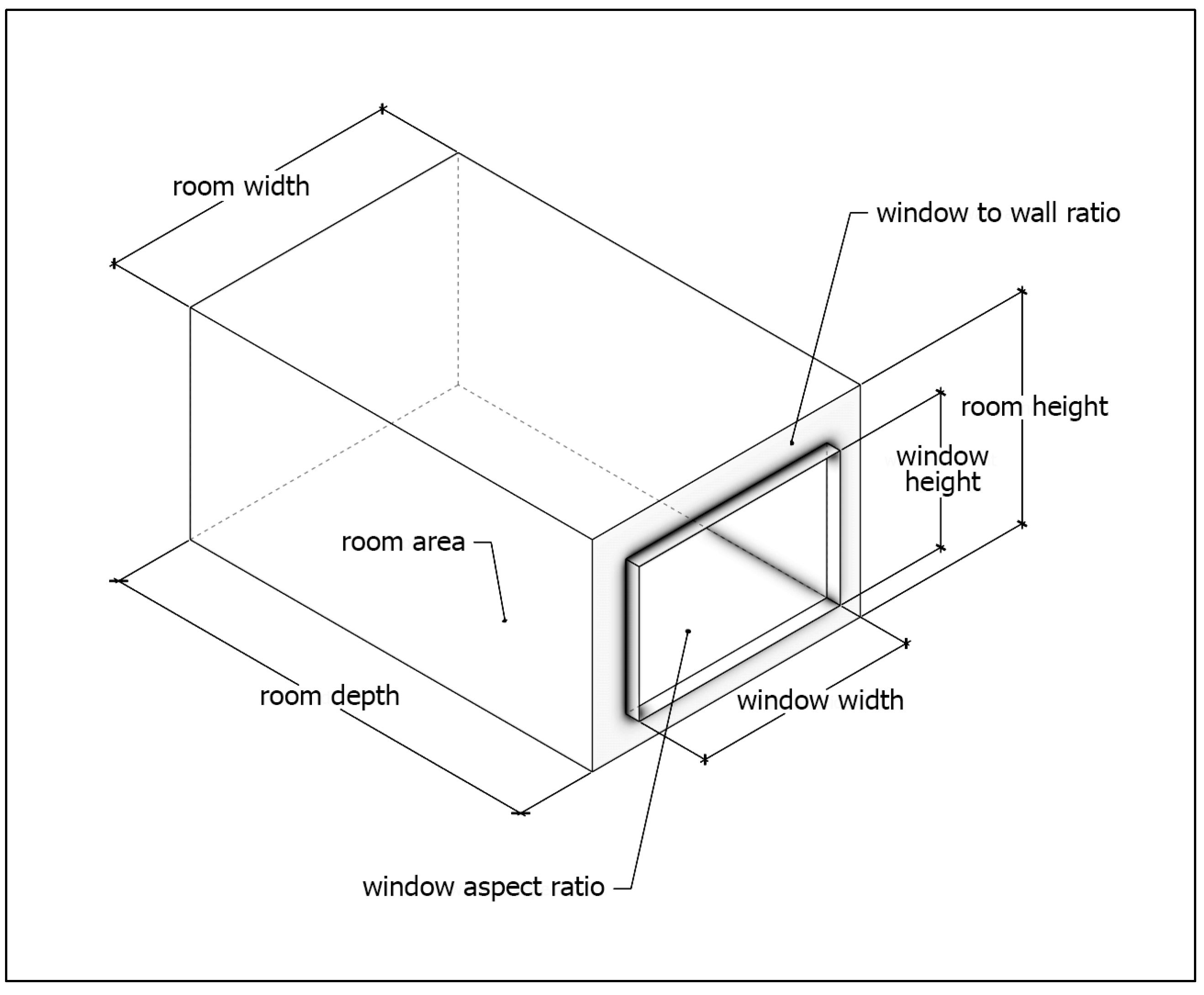
For an office space with a range of possible configurations, daylight performance is likely to be affected by several factors, including climate, orientation, room layout, window configuration, and surface reflectance. In this study, the input parameters were selected based on design considerations of the basic geometry, which designers typically adjust during the early stages of the design process, while all other parameters were kept constant. Four geometry-related parameters were used as inputs to the ML model, these being room dimensions, room area, window aspect ratio, and window-to-wall ratio. Figure 3 illustrates the 3D parametric model used in the training process, while

Table 2. Design variables with associated range and steps (in meters).

Parameter	Range	Steps
Room width	3–9	2
Room depth	3–9	2
Room height	3	-
Window width	1–9	1
Window height	1–3	1

details the design variables along with their respective ranges and step sizes.

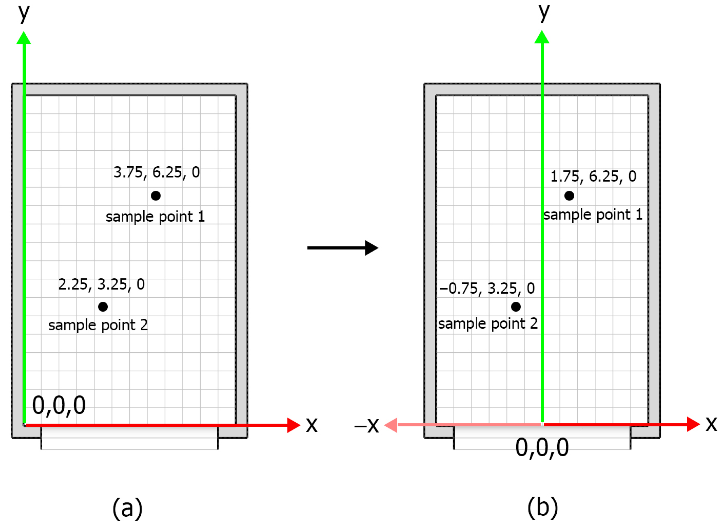
One of the challenges in developing the model was managing the variation in room sizes and the distribution of sensor points. Rooms of different sizes generated varying numbers of sensor points, leading to inconsistent numbers of target outputs per room. To address this issue, a method was proposed that involved engineering the spatial features of the sensor points by repositioning and normalizing their positions relative to a local coordinate system specific to each room. As illustrated in Figure 4a, the local coordinate system was initially defined with its origin at the bottom-left corner of the room. However, this approach resulted in values being skewed toward the left side of the room as room sizes varied, leading to potential inconsistencies and symmetrical inaccuracies in predictions. To reduce the impact of this effect, the origin of the coordinate system was shifted along the X-axis to align with the centerline of the window, as shown in Figure 4b. This modification ensured a symmetrical distribution of sensor points, eliminating discrepancies. Subsequently, normalization was performed by dividing the X and Y values by the room’s width and depth, respectively. This process ensured consistency across rooms of varying sizes, making the relative positions of the sensor points independent of the room’s dimensions.

The output includes the Daylight Factor (DF) and Useful Daylight Illuminance (UDI), with the latter evaluated within the range of 100 to 3000 lux (UDI-autonomous). Modifying the parameters within the specified ranges resulted in a simulation dataset comprising 288 models, each parametrically generated from the base case and serving as an empirical ground truth for the machine learning model.

3.2. Network Architecture and Training Process

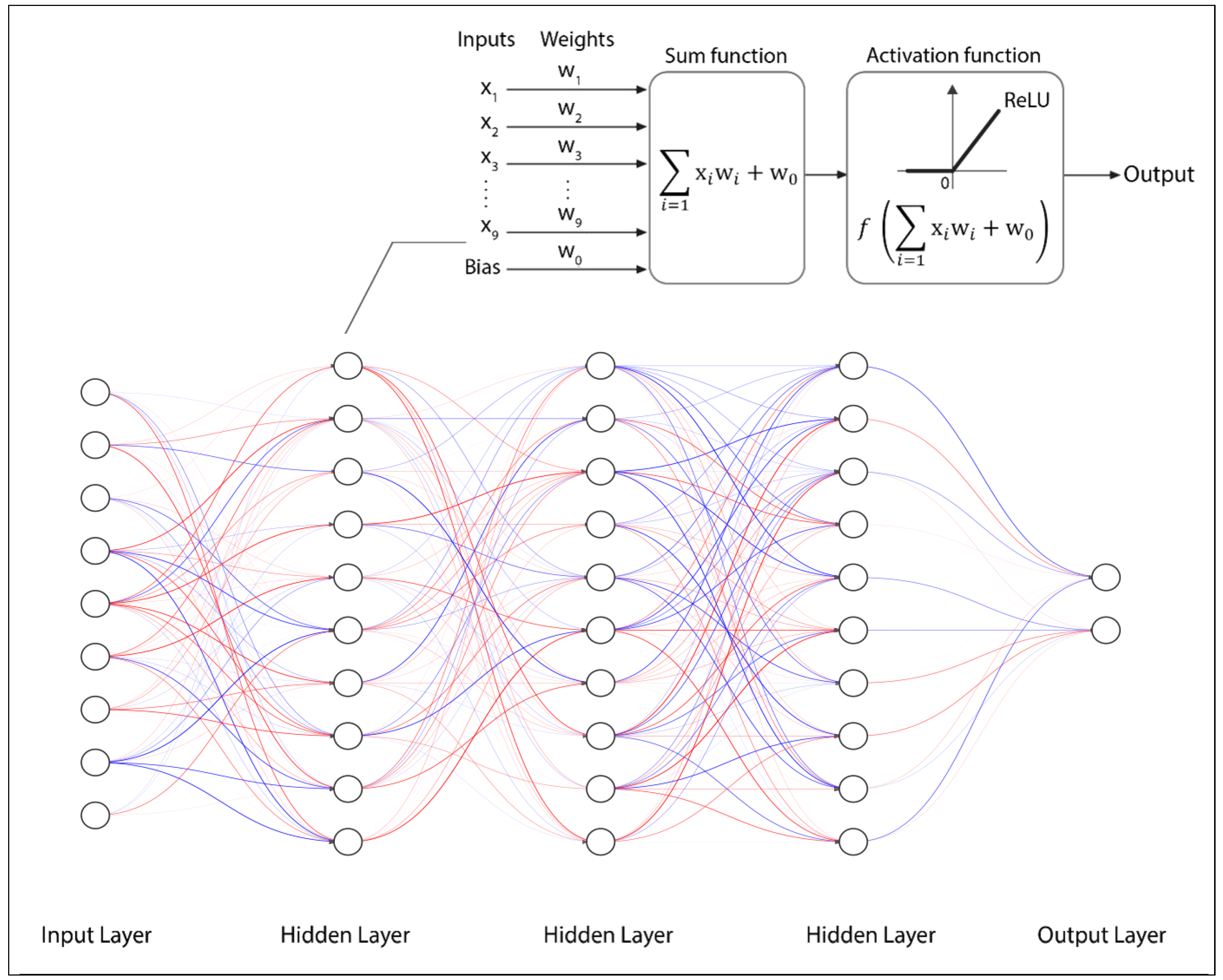
DayANN architecture consists of five layers, where each layer applies weights and activation functions to transform input into output in a single forward pass. The layers include an input layer, three hidden layers, and an output layer. Each neuron in a layer performs a weighted sum of its inputs, adds a bias term, and passes the result through the Rectified Linear Unit (ReLU) activation function to produce its output, as illustrated in Figure 5. Formally, the transformation at each layer $l$ is expressed as follows:

$$a^l=\sigma \left(W^{\left(l\right)a^{l-1}}+b^l\right)$$

(1)

where $a^l$ is the activation vector, $W^{\left(l\right)}$ is the weight matrix, and $b^l$ is the bias vector. The nonlinearity is introduced via the Rectified Linear Unit (ReLU) activation function. The term $\sigma$ in the formula below represents the activation function that introduces nonlinearity into the model. For any input value $z$ (representing the weighted sum of inputs plus bias), the function output is determined as follows:

$$\sigma \left(z\right)=\max \left(0, z\right)$$

(2)

The full network architecture is defined as follows:

▪

Input Feature Vector $x$: A 6-dimensional vector consisting of room and window geometry parameters plus normalized sensor coordinates. Output Vector ŷ: A 2-dimensional vector [UDI, DF], representing the predicted Useful Daylight Illuminance (300–3000 lux range) and Daylight Factor for each sensor point.

$$\mathrm{ŷ}=\left[UDI, DF\right]\in {\mathbb{R}}^2$$

(3)

▪

Hidden Layer Configuration: Three hidden layers containing 64, 32, and 16 neurons, respectively.

▪

Regularization: A dropout rate of 0.3 is applied during training to prevent overfitting on the 288-case dataset.

During training, dropout stochastically sets each neuron’s output to zero with probability p = 0.3, formally defined as ã = m ⊙ a, where m ~ Bernoulli(1 − p) is a binary mask.

$$ã=m\odot a, m ~ Bernoulli\left(1-p\right)$$

(4)

The weights are iteratively updated in 16 batches to reduce the overall loss. For each batch, the backpropagation algorithm computes the gradients with respect to the weights in the network. DayANN is implemented in Python (version 3.10.8) using the TensorFlow and Keras libraries and trained on the simulation dataset.

This specific configuration was adopted based on the characteristics of the input data, which comprises tabular, parametric features such as window dimensions, room area, and geometric layout variables. Unlike image-based datasets that possess local spatial correlations, these discrete variables are better suited for a feedforward structure than for convolutional neural networks (CNNs). During the development phase, various multi-layer perceptron (MLP) configurations were tested, including deeper architectures. It was observed that increasing the depth beyond three hidden layers yielded no significant gains in predictive accuracy; rather, it heightened the risk of overfitting, particularly considering the dataset size of 288 cases. Consequently, a three-layer hidden structure was selected to provide an optimal balance between capturing the nonlinear complexities of daylighting and maintaining model robustness. This architectural choice is further reinforced by hyperparameter tuning and the use of early stopping, consistent with established methodologies in daylighting research that utilize neural networks for parametric performance prediction.

Once the network architecture was developed, a set of hyperparameters was identified along with their corresponding values for testing. This included, but was not limited to, the number of epochs, dropout rate, batch size, and the optimizer learning rate. The model was trained using the Adam optimizer with a learning rate of 0.001. The mean squared error (MSE) was employed as the loss function, formally defined as

$$L\left(W\right)={\displaystyle \frac{1}{N}}{\sum }_{i=1}^N{\left({\mathrm{ŷ}}_{\mathrm{i}}-y_i\right)}^2$$

(5)

where ŷ_i is the predicted output, and y_i is the simulated ground truth for the $i$th sample. The network weights are updated via backpropagation using the gradient descent rule:

$$W\leftarrow W-\alpha ·{\nabla }_{W}L\left(W\right)$$

(6)

where $\alpha$ is the learning rate and ${\nabla }_{W}L$ is the gradient of the loss with respect to $W$.

To reduce the risk of overfitting, an early stopping callback was implemented, and a dropout rate of 0.3 was applied. An early stopping patience of 10 was set, with the number of epochs fixed at 200. To ensure the neural network is replicable, it was designed to be streamlined, with most hyperparameters set to standard values recommended in the literature. The tuned parameters are presented in

Table 3. Hyperparameters of the training model.

Hyperparameter	Value
Epochs	200
Batch size	16
Learning rate	Initial value: 0.001 Drop rate: 0.3
Hidden layers	3
Loss function	MSE
Activation function	ReLU
Optimizer	Adam
Patience	10

.

The hyperparameters of DayANN were defined prior to training based on preliminary experimentation and remained fixed throughout the training process. Model convergence was monitored using a validation subset, and an early stopping mechanism with a patience of 10 epochs was applied to prevent overfitting. If no improvement in validation loss was observed for ten consecutive epochs, training was terminated, and the best-performing model weights were retained. All computations were performed on an NVIDIA GeForce RTX 4080 GPU and an Intel Core i9 processor.

Deep neural networks are effective at modeling complex relationships, but their lack of transparency regarding the influence of individual input variables can be a limitation. To overcome this, SHAP (Shapley Additive Explanations) was applied, providing a consistent quantification of each input feature’s contribution to the model’s output. In the context of daylight analysis, SHAP values reveal how much each design parameter (e.g., window width, room depth) affects the predicted outcome for a given scenario, either increasing or decreasing it relative to the average. SHAP quantifies these contributions by systematically evaluating all possible subsets of input variables and assessing the change in the model’s prediction when a specific feature is included in each subset. For every subset, the marginal contribution of the feature is computed, and the resulting Shapley value is derived as the weighted average of these marginal contributions across all possible permutations of feature inclusion. This approach provides a consistent decomposition of the model’s output, enabling a precise quantification of how each individual input drives the final prediction. Although SHAP can explain individual predictions, this study reports aggregated feature importance to highlight the most influential variables overall.

3.3. Performance Predictors

The predictive performance of the machine learning model is compared to that of simulation-based models, with results evaluated using a range of performance metrics, including the coefficient of determination (R²), mean squared error (MSE), mean absolute error (MAE), and root mean squared error (RMSE), consistent with those employed in previous research. These can be expressed in the following equations:

$$R^2=1-{\displaystyle \frac{ {\sum }_{i=1}^N{\left({\mathrm{ŷ}}_i-y_i\right)}^2 }{{\sum }_{i=1}^N{\left(y_i-\overline{y}\right)}^2}}$$

(7)

$$MSE={\displaystyle \frac{1}{N}} \sum _{i=1}^N{\left({\mathrm{ŷ}}_i-y_i\right)}^2$$

(8)

$$MAE={\displaystyle \frac{1}{N}} \sum _{i=1}^N\left|{\mathrm{ŷ}}_i-y_i\right|$$

(9)

$$RMSE=\sqrt{{\displaystyle \frac{1}{N}} \sum _{i=1}^N{\left({\mathrm{ŷ}}_i-y_i\right)}^2}$$

(10)

where ${\mathrm{ŷ}}_i$ is the predicted value, $y_i$ is the actual ground truth value for the $i$th data sample (out of N data samples), $\overline{y}$ is the mean of the actual ground truth values, and N is the number of data samples in the testing dataset.

4. Results and Discussion

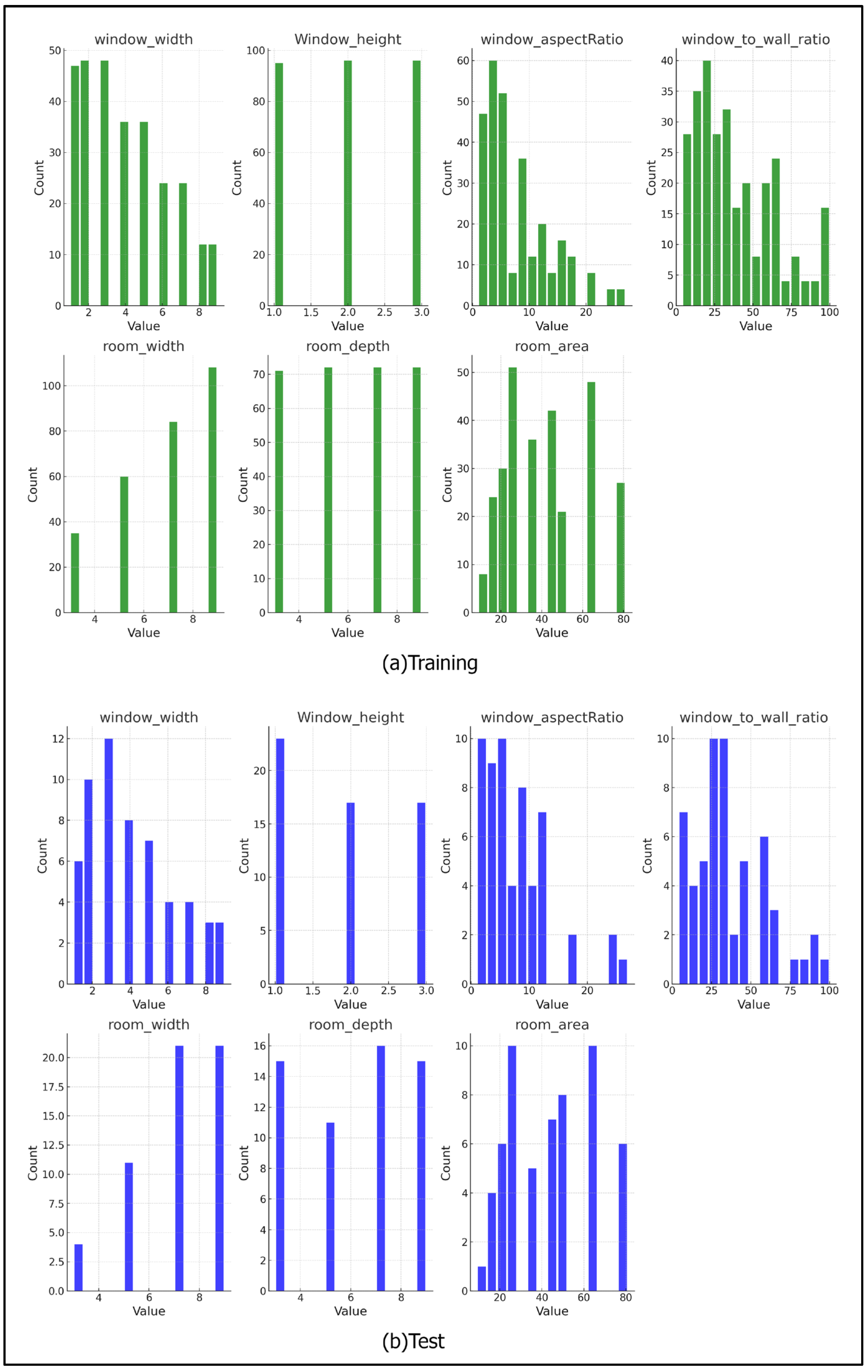
A summary of the results is presented to enable direct comparison between simulation-based and ML-based models. Figure 6 presents histograms illustrating the distribution of input variables aggregated across the training and testing subsets in each fold during 5-fold cross-validation. In the training dataset, window width and room width demonstrate relatively uniform distributions, whereas window aspect ratio and window-to-wall ratio exhibit more skewed distributions, with higher frequencies observed at lower values. Similar patterns are observed in the testing dataset, where the distributions of the input variables closely align with those of the training dataset. These consistent patterns across both datasets suggest that the training and testing datasets are representative of the same underlying data distribution, which is essential for reliable model evaluation and generalization [42,43].

Table 4. Average performance metrics (±standard deviation) of the model across 5-fold cross-validation.

Metric	MAE	RMSE	R2	Relative Error %
UDI (300–3000)	0.0262 ± 0.0014	0.0366 ± 0.0021	0.988 ± 0.003	5.07 ± 0.22
DF	0.0438 ± 0.0025	0.0617 ± 0.0034	0.947 ± 0.006	8.55 ± 0.41

presents summary statistics comparing DayANN predictions with the simulated daylight results. For UDI (300–3000 lux), the models achieved an MAE of 0.0262, an RMSE of 0.0366, and an R² value of 0.988, with a relative error of 5.07%. For Daylight Factor (DF) predictions, the models achieved an MAE of 0.0438, an RMSE of 0.0617, and an R² value of 0.947, with a relative error of 8.55%. These results highlight the robustness of DayANN in accurately predicting daylighting metrics, a result similar to that produced in previous studies. The practical significance of these error metrics should be evaluated within the framework of architectural design decision-making. Given that R² values exceed 0.94 and the MAE/RMSE remain low relative to the total range of UDI and DF, the model demonstrates a high degree of reliability for early-stage design. Beyond predictive accuracy, the principal advantage of DayANN lies in its computational efficiency compared to traditional simulation-based workflows. The capacity to provide near-instantaneous performance feedback facilitates its integration into iterative parametric design processes, where computational speed is as critical as numerical precision for effective design exploration.

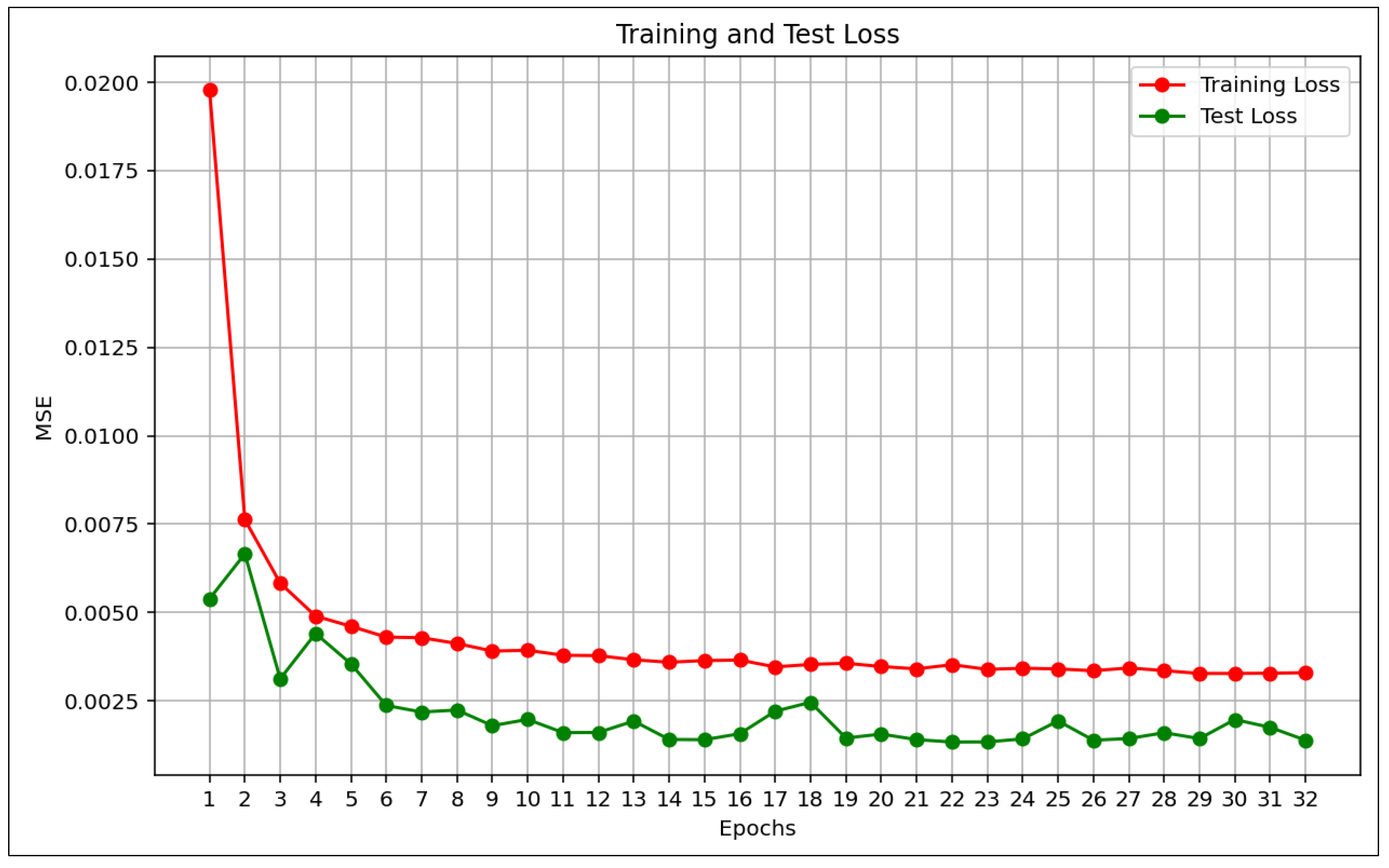
The training and validation loss curves plotted in Figure 7 represent one fold from the five-fold cross-validation process. Early in the training process, the loss decreases rapidly but then plateaus by epochs 4 and 6, respectively. As the number of epochs increases, both training and validation losses stabilize, indicating convergence of the model without substantial divergence between the two curves. Notably, minor fluctuations in early test loss values (epochs 1–4) are observed; however, these do not correspond to sustained divergence between training and validation curves, indicating stable generalization. 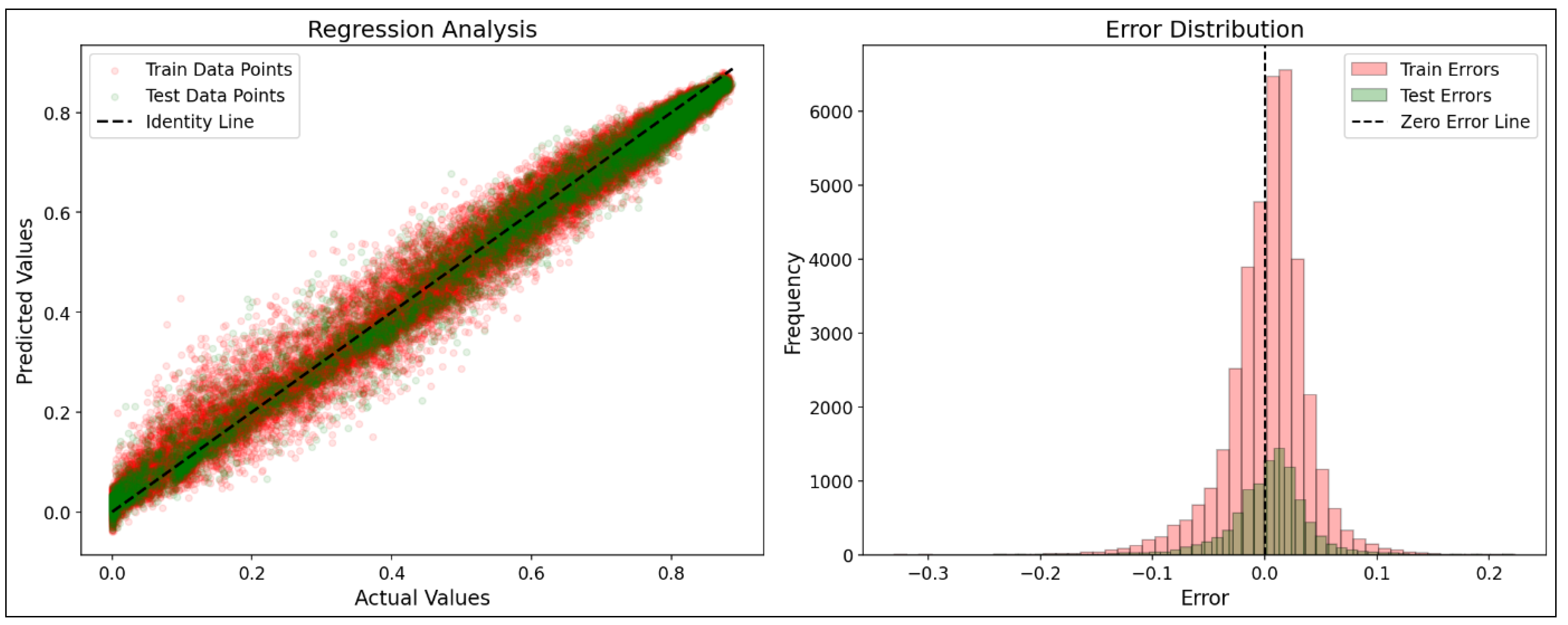Figure 8 shows that the model achieves strong predictive performance on both training and validation data in a representative fold, with no substantial overfitting evident from the regression and error distribution plots.

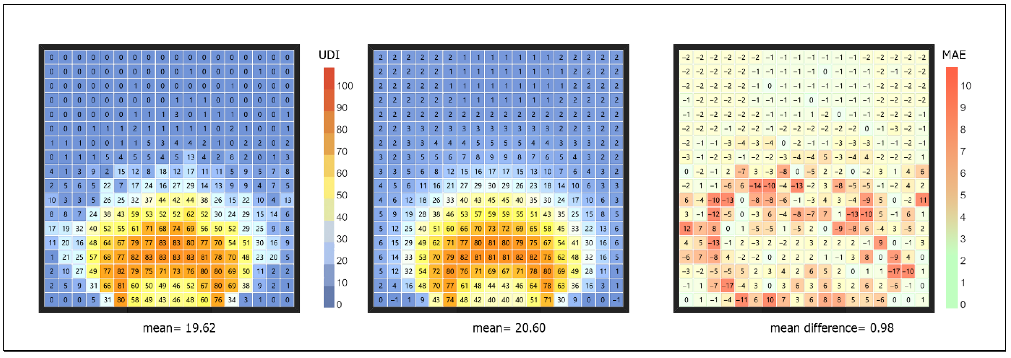
Figure 9 presents the case with the highest error, identified from the extreme values observed in the dataset, to illustrate the spatial distribution of prediction discrepancies. In this scenario, the largest deviations are concentrated in transitional daylight zones, where illuminance levels shift rapidly from high values near the window to lower values deeper within the room. Such regions are inherently sensitive to nonlinear interactions between geometric parameters, particularly window width and room depth, which jointly influence daylight penetration gradients. The observed discrepancies may, therefore, reflect the difficulty of approximating steep spatial gradients within a relatively small training dataset. In addition, a slight systematic underestimation of UDI values is observed across several cases. This tendency may be attributed to the smoothing behavior of the feedforward architecture when modeling sharp transitions in illuminance distribution. Despite these localized deviations, the model successfully captures the overall spatial structure and trend of daylight distribution, and extreme errors remain isolated rather than spatially clustered, limiting their practical impact on design-level decision-making.

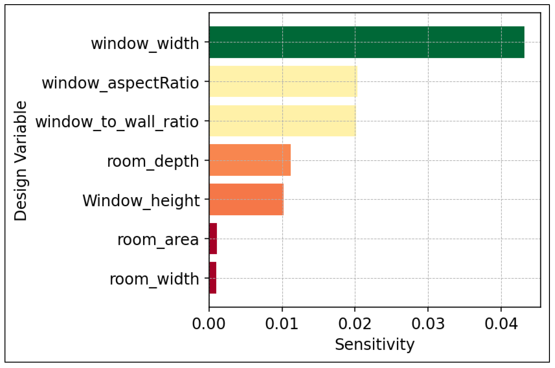
The results of the sensitivity analysis reveal that the window width parameter by far has the greatest impact on the model output variance across all input variables. Figure 10 illustrates the feature importance for the model, with the features ranked in descending order, where the top-ranked feature is the most influential on the model’s predictions. Window-related variables have a significant influence on the model, whereas room dimensions and area have a relatively minor impact. An examination of the SHAP values indicates that the influence of these parameters is inherently nonlinear and characterized by significant interdependencies. For example, the impact of window width is closely coupled with room depth; in shallower rooms, window width significantly drives daylight penetration, whereas in deeper configurations, its marginal influence diminishes as internal reflections become the secondary dominant factor. This behavior aligns with established daylighting principles, where the effectiveness of an aperture is physically constrained by the room’s geometric proportions. These insights allow for a strategic prioritization of design variables, enabling a more focused approach to model development by identifying the critical parameters that drive daylight distribution. By recognizing these nonlinear thresholds and feature interactions, less influential variables can be assigned fixed values or simplified, allowing designers to concentrate on the most sensitive parameters during the early stages of the design process. Furthermore, the alignment between the model’s learned sensitivities and known physical logic substantiates the reliability of DayANN as a physically plausible surrogate for complex daylight simulations.

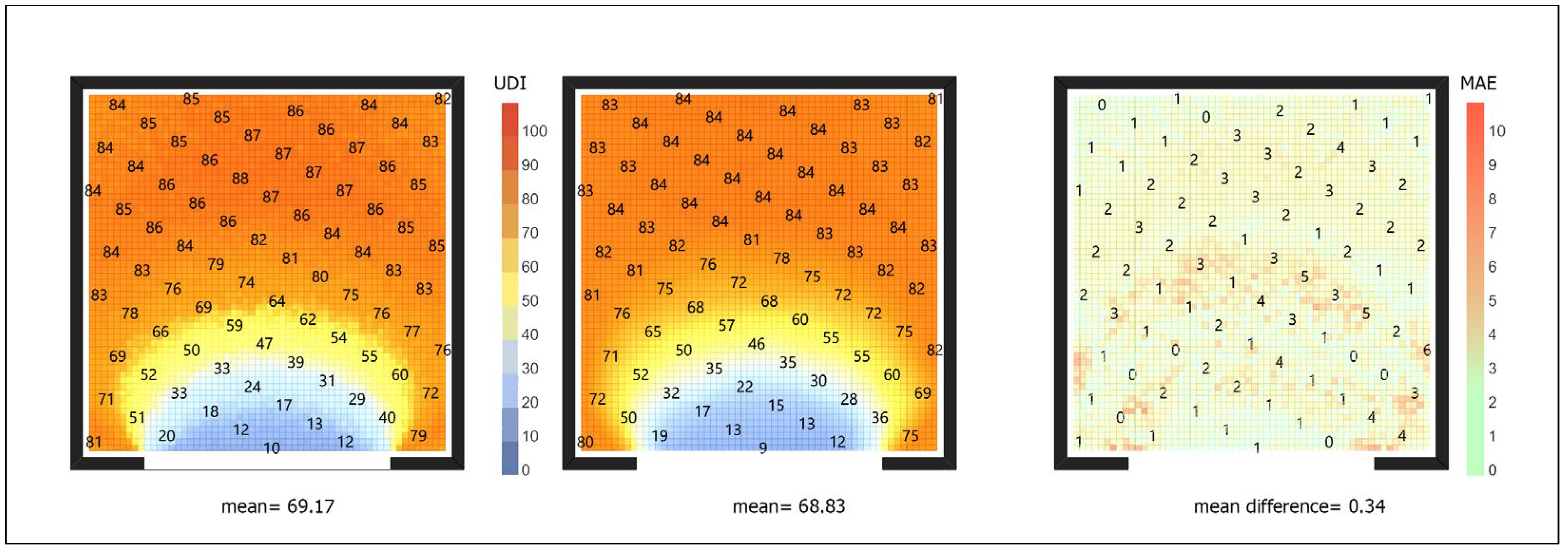
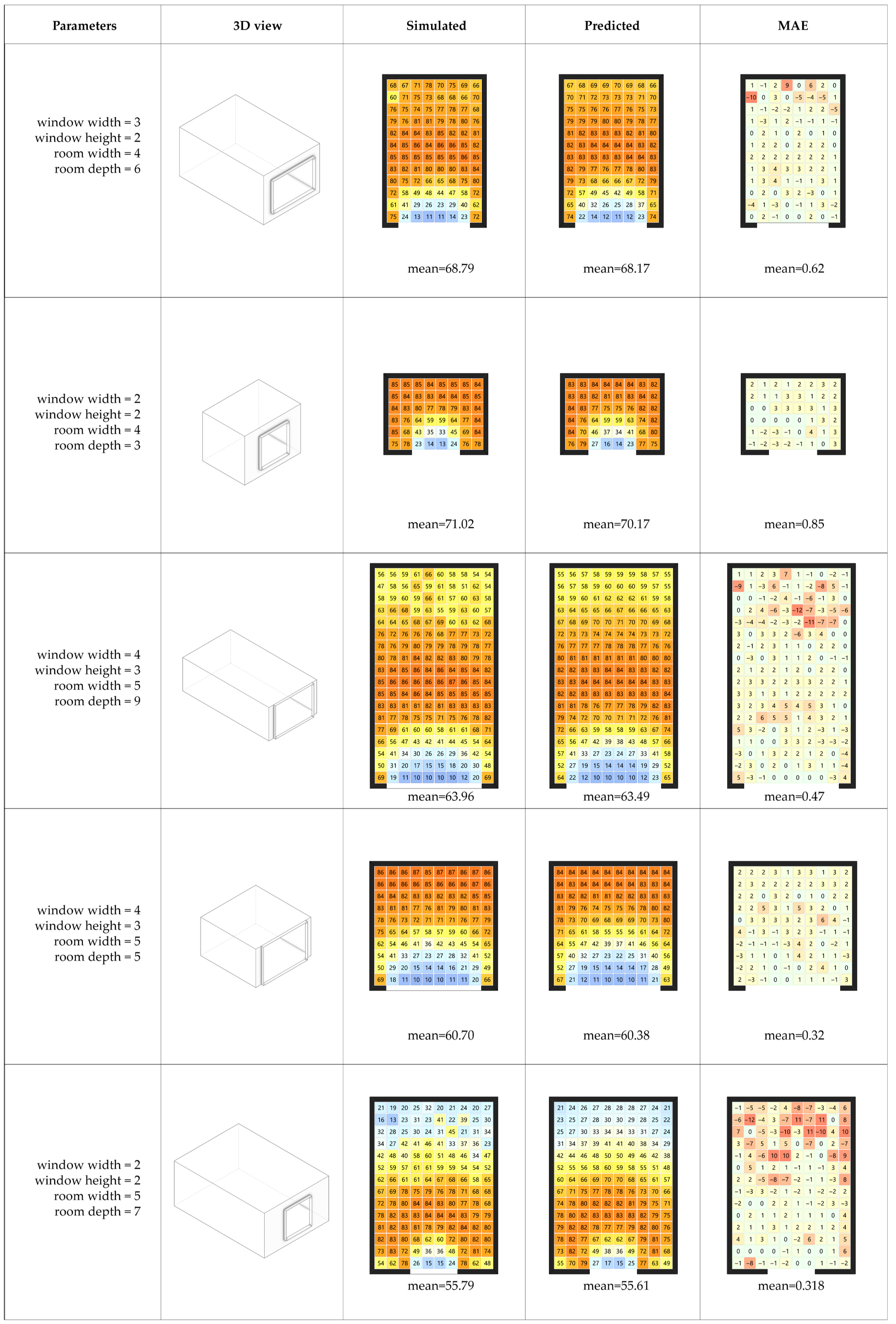
To provide a more comprehensive assessment of model performance, several representative cases were randomly selected from the test set and are presented in Figure 11. Across all cases, the simulated UDI values tend to be slightly higher than the predicted values, but the differences are minimal, typically within a small decimal margin. These results confirm the model’s ability to accurately capture the spatial patterns of daylight distribution under varying geometric conditions.

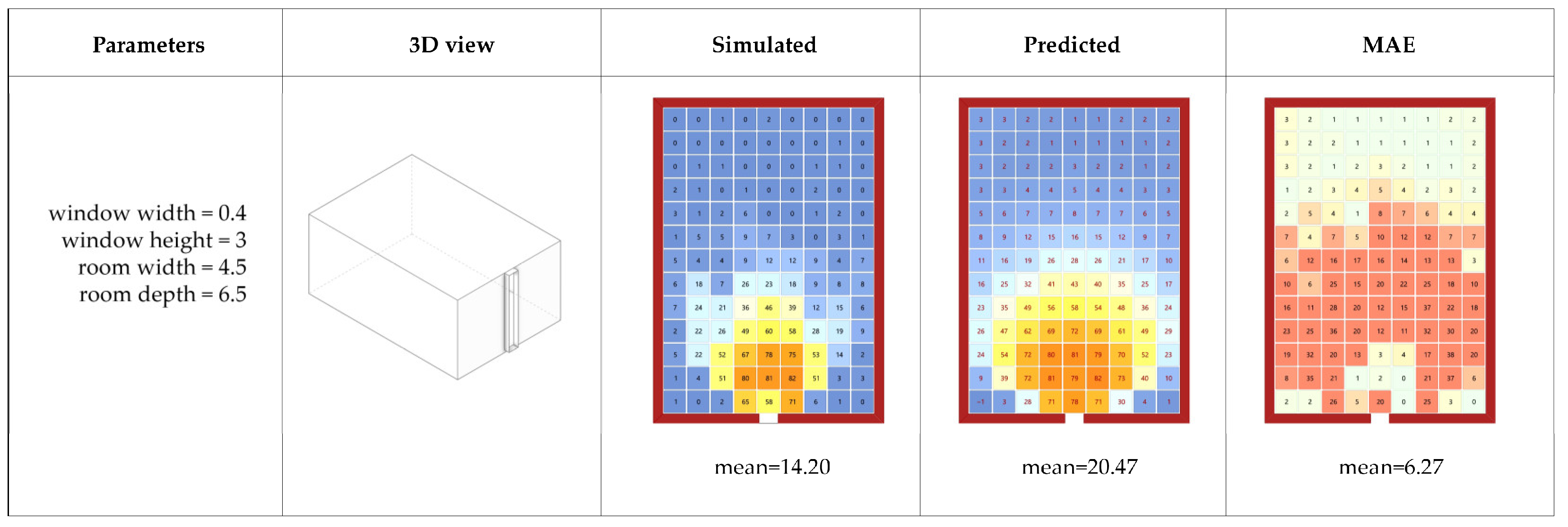
Following the cases in Figure 11, Figure 12 presents an extreme example from the dataset, characterized by a narrow and tall window configuration. The simulated UDI distribution indicates low daylight availability throughout most of the room, whereas the predicted UDI values are generally higher, indicating a localized overestimation in this extreme configuration. The largest discrepancies are observed in the area near the window, resulting in a mean difference of 6.27.

When the UDI patterns are examined at high resolution with an analysis grid spacing of 0.1 m, the simulation results display greater variability and more discrete transitions, while the model predictions are generally smoother, as illustrated in Figure 13. Given the relatively small size of the simulation dataset (288 samples), a 5-fold cross-validation approach was adopted to ensure a statistically robust evaluation. This method reduces the risk of overfitting to a single partition and provides a more reliable measure of the model’s generalization capability under varying geometric configurations.

Although the current scope of this research is centered on establishing DayANN as a reliable surrogate for computationally intensive simulations, the necessity of this architecture is supported by its ability to generalize across the parametric design space with high precision (R² > 0.94). While direct comparative experiments with alternative ML models are intended for future stages of this research to further demonstrate the computational advantages of DayANN, the current validation against empirical ground truth serves as the foundational step in confirming the model’s reliability.

5. Conclusions

This paper presented the implementation and performance evaluation of DayANN (Daylight Artificial Neural Network), a deep neural network for daylight prediction in a side-lit office space with varying geometric configurations. By training on a simulation dataset of 288 parametrically generated cases, the aim of this study was to develop a model capable of accurately predicting daylight performance across a range of design scenarios. A network architecture comprising three hidden layers proved effective, producing strong performance in terms of predictive accuracy and error metrics. The results are consistent with previous studies, confirming that the selected input parameters enable accurate daylight predictions while preserving the overall spatial distribution characteristics. The predictions of the machine learning model, while generally smoother than those from simulation, remained consistent across a range of design scenarios and did not exhibit substantial overfitting across the evaluated scenarios.

The results indicate that DayANN achieves strong predictive performance, with R² values exceeding 0.94 for both Daylight Factor (DF) and Useful Daylight Illuminance (UDI) under 5-fold cross-validation. The reported MAE and RMSE values suggest that prediction deviations remain within ranges that are acceptable for early-stage architectural decision-making, where comparative evaluation of design alternatives is often more critical than exact numerical precision. Sensitivity analysis further highlights the dominant influence of window-related parameters, particularly window width, reinforcing established daylighting principles and demonstrating that the learned relationships are physically plausible.

Beyond predictive accuracy, the principal contribution of this study lies in the development of a structured and automated Grasshopper-to-machine learning workflow. By enabling rapid surrogate prediction in place of repeated simulation runs, the framework supports iterative parametric exploration during conceptual design phases. In practical terms, this allows designers to evaluate multiple geometric alternatives in substantially shorter timeframes, facilitating informed decision-making without the computational burden of full daylight simulations at every iteration.

Nevertheless, several limitations must be acknowledged. The model was trained on a single side-lit office typology with a defined range of geometric parameters. While the methodology is transferable, predictive reliability may vary for alternative room configurations, complex façade systems, or urban contexts with external obstructions. Additionally, extreme geometric scenarios, particularly those producing sharp daylight gradients, may yield slightly higher localized prediction errors. Future research should therefore expand the dataset scope, incorporate additional architectural variables, and benchmark multiple machine learning architectures to further evaluate generalization capacity and robustness.

Overall, DayANN demonstrates that a streamlined deep neural network, when embedded within an integrated parametric workflow and complemented by interpretability analysis, can function as a computationally efficient and transparent surrogate model for daylight performance estimation in early-stage design applications.