Peak Strain Prediction and Fragility Assessment of Buried Pipelines Subjected to Normal-Slip and Reverse-Slip Faulting

Abstract

Permanent ground deformation caused by fault movement threatens the safe operation of buried pipelines. Accurate fragility assessment of buried pipelines subjected to faulting is essential for pipeline design and risk management. However, buried pipelines exhibit nonlinear mechanical responses due to the coupled effects of multiple factors. Moreover, the effects of key parameters remain insufficiently quantified, limiting the accuracy and engineering applicability of existing fragility assessments. In this study, a three-dimensional finite element model incorporating large deformation and nonlinear pipe–soil interaction is developed and validated against representative experimental data. Using this model, numerical simulations are performed for 352 parameter combinations covering fault type, dip angle, burial depth, soil type, and pipe material. Nonlinear regression of the simulation results yielded predictive models for pipeline peak axial strain under normal-slip and reverse-slip faulting. A fragility framework is then established with fault displacement as the intensity measure, and fragility curves are derived for both faulting modes. The predicted peak axial strains agree with the finite element results: 78.6% (normal-slip) and 72.5% (reverse-slip) of predictions fall within ±20% error. The fragility curves enable quantitative estimation of fault-displacement thresholds. In the case study, the intact-to-damage displacement threshold is approximately 0.6 m for normal-slip faults but approximately 0.2 m for reverse-slip faults, indicating a higher failure likelihood under reverse-slip faulting. Within the investigated parameter ranges, the fault dip angle is the most significant factor affecting the pipeline failure probability for both normal-slip and reverse-slip faulting. Sandy soil and greater burial depth substantially increase the probability of moderate-to-severe damage, whereas higher steel grade increases the displacement threshold for transition from intact to failure. This study provides a rapid quantitative tool and a theoretical basis for pipeline design and risk quantification of buried pipelines in fault zones.

1. Introduction

Pipelines are critical infrastructure for global energy transmission, owing to their wide spatial distribution and extensive network length [1]. Many long-distance oil and gas pipelines cross active fault zones, where fault displacement can produce substantial permanent ground deformation (PGD) [2] and thereby threaten pipeline structural integrity. In particular, reverse-slip and normal-slip faulting can be especially damaging, potentially causing pipe-wall buckling or localized tensile rupture. Accurate assessment of deformation and failure risk in buried pipelines subjected to fault movement is essential to improve the resilience of energy infrastructure and reduce disaster losses.

Fragility curve-based probabilistic risk assessment has been increasingly adopted for pipeline design and risk assessment of buried pipelines. These studies typically use permanent ground deformation (PGD) or fault displacement as the intensity measure (IM). Using strain-based damage indices tied to performance states (e.g., yielding, local buckling, and rupture), researchers develop fragility curves or surfaces that relate failure probability to the IM via extensive numerical simulations or response-surface methods [3,4]. Ni et al. [4,5] applied machine learning approaches to fragility analysis of pipelines subjected to fault displacement and quantified the key parameters governing fragility. Overall, existing fragility studies mostly focus on transverse PGD or typical strike-slip fault conditions, while systematic research on fragility characteristics under normal-slip and reverse-slip faults, different fault parameters, and various combinations of key pipeline parameters remain insufficiently explored.

Peak-strain prediction models are central to pipeline fragility analysis. Prior studies have leveraged extensive finite element results to develop peak-strain prediction models for rapid engineering assessment [6,7]. These models typically use fault displacement, diameter-to-thickness ratio, burial depth, and the pipe–soil stiffness ratio as key predictors, and they derive explicit regression equations for peak axial tensile and compressive strains that can be directly applied in strain-based design and verification [8]. Accurate prediction of the mechanical response of buried pipelines under fault movement is therefore critical to developing reliable peak-strain models.

In recent years, computationally efficient approaches for response prediction and probabilistic assessment of buried pipelines have received increasing attention, driven by the need for multi-query evaluations in parametric studies and uncertainty-based risk assessment. For example, Zheng et al. proposed an easy-to-implement probabilistic assessment framework by integrating a finite-difference-based strain calculation tool with Monte Carlo simulation (MCS) to estimate the probability of strain capacity exceedance for pipelines subjected to permanent ground movement [9]. In parallel, physics-informed neural networks (PINNs) have emerged as promising surrogate solvers for PGD-induced pipeline responses: recent studies demonstrated that PINN predictions can closely match conventional numerical solutions while offering notable efficiency advantages in multi-query scenarios after training [10]. Furthermore, a PINN-based reliability analysis framework (PINN-RA) was recently introduced by integrating a parametric PINN surrogate model with MCS, enabling efficient reliability assessment while accounting for uncertainties in ground movement and soil properties [11]. These advances provide valuable perspectives on coupling response prediction with probabilistic assessment and motivate the development of efficient, engineering-oriented models that can be readily combined with fragility analysis.

Despite these encouraging developments, the choice of an appropriate modeling strategy still depends on the target application and the dominant nonlinearities. Finite element models remain the most general approach for capturing three-dimensional pipe–soil interaction, large deformation, contact nonlinearity, and material nonlinearity, but they are often computationally demanding for extensive parametric or probabilistic studies. Finite difference-based tools are attractive due to their simplicity and efficiency, yet they are typically formulated within idealized beam/spring representations and can be discretization-dependent [10]. PINN/PINN-RA approaches provide a promising mesh-free surrogate route once trained, but their implementation still requires careful formulation, training, and validation across parameter ranges [11]. Motivated by these efforts, the present study aims to provide a complementary, engineering-friendly pathway: we leverage a validated 3D pipe–soil coupled FE model to generate a comprehensive database for normal-slip and reverse-slip faulting, then we develop explicit regression-based peak axial strain prediction equations that are straightforward for design checks and can be directly integrated with fragility curves for risk quantification.

The FE model is an important tool for investigating the mechanical response of buried pipelines subjected to fault displacement [12], and numerous studies have been conducted. Liu et al. [7,13] used the soil-spring method to represent soil–pipe interaction and investigated pipeline response and peak-strain prediction under strike-slip and reverse faulting. However, the soil-spring method idealizes pipe–soil interaction as linear springs and may unrealistically allow the soil to carry tension, which limits its ability to capture the system’s nonlinear behavior. As a result, it is often unsuitable for large-deformation scenarios such as fault movement, which can introduce substantial errors in response prediction and failure-risk assessment. In contrast, pipe–soil coupled finite element models directly simulate pipeline–soil interactions using continuum (solid) elements and contact algorithms. With large-deformation kinematics, elastoplastic constitutive models, and contact–friction formulations, such models can more realistically capture tensile, compressive, and bending behavior during fault movement [14,15]. For example, Vazouras et al. developed coupled models for X65 and X80 pipelines under strike-slip faulting and examined the effects of soil type, pipe geometry, and crossing angle on failure [16,17]. Zhang et al. evaluated how fault displacement influences local buckling [18]. Nevertheless, research on the mechanical response of buried pipelines under normal-slip and reverse-slip faulting remains limited. Moreover, systematic quantitative assessment of the coupled effects of fault and pipeline parameters on peak axial strain is scarce, hindering the development of robust fragility curves for buried pipelines subjected to fault movement.

This study develops a three-dimensional pipe–soil coupled finite element model that accounts for large deformation and contact nonlinearity. Using this model, mechanical response analyses were conducted for pipelines subjected to normal-slip and reverse-slip faulting across fault dip angles, displacement levels, soil types, and pipeline parameters, and the influence of key factors on axial strain was quantified. Based on the simulation results, separate peak axial strain prediction models for normal-slip and reverse-slip faults were derived, and their accuracy was validated against the finite element results. Fragility curves for buried pipelines subjected to fault movement were further developed to quantify the effects of fault type, dip angle, and pipeline properties on fragility, thereby providing a basis for pipeline design and risk assessment of pipelines crossing active faults.

2. Numerical Simulation Method and Verification

2.1. Finite Element Model

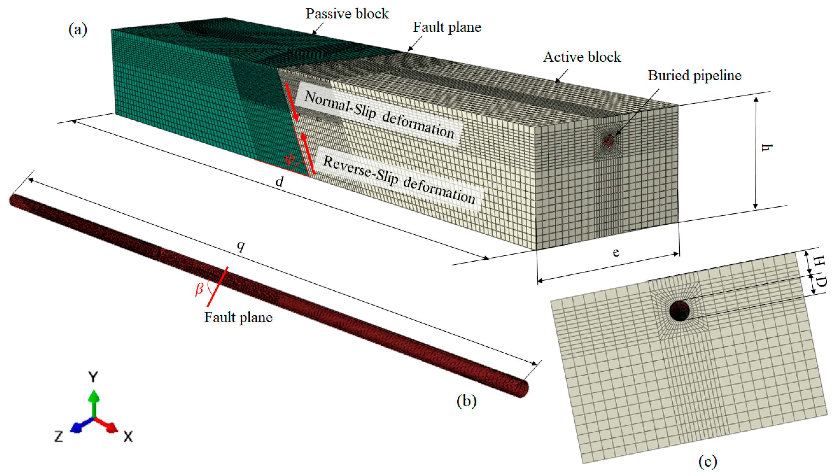
Based on the geometric parameters in

Table 1. Dimensions of research objects and simulation cases.

	d/m	e/m	h/m	q/m	Crossing Angle β/°	Dip Angle ψ/°	Pipeline Material	Soil Type	Diameter D (Thickness t)/mm	Soil Displacement/m	Buried Depth H/m
Normal-slip faulting	80	15	10	80	90	45, 75	X80, X60	Sand, Clay	406 (10), 864 (22)	0–3	1 4.5
Reverse-slip faulting	80	15	10	80	90	45, 75	X80, X60	Sand, Clay	406 (10), 864 (22)	0–1	1 4.5

, a three-dimensional pipe–soil coupled finite element model of a buried pipeline subjected to fault movement was developed (Figure 1). The model consists of an active block, a passive block, and a buried pipeline, with the passive block subjected to fixed boundary conditions on its surface, as shown in the boundary conditions in Figure 2. Both tectonic blocks are active in nature; the term ‘passive block’ is used here only to denote the block where fixed boundary conditions are applied in the FE model. The angle between the pipeline axis and the fault plane is defined as the crossing angle, β. The model was solved using ABAQUS/Standard (v2016). The mesh employed C3D8R eight-node, reduced-integration solid elements. To improve local accuracy, the mesh was refined (i) within 3 m of the pipeline in both blocks and (ii) within 10 m on either side of the fault. In the refined regions, the target element size was 0.2 m; elsewhere, it was 0.4 m. The pipeline was also refined within 10 m on either side of the fault (0.2 m element size), with a 0.4 m size in the remaining sections. At least five elements were used through the pipe-wall thickness.

To investigate the influence of parameters such as fault dip angle, pipe grade, soil type, pipe diameter, fault displacement, and burial depth on the mechanical response of pipelines under fault movement, parametric simulations were conducted. In total, 352 finite element simulations were performed, providing the dataset used to develop the peak axial strain prediction model.

2.2. Constitutive Model

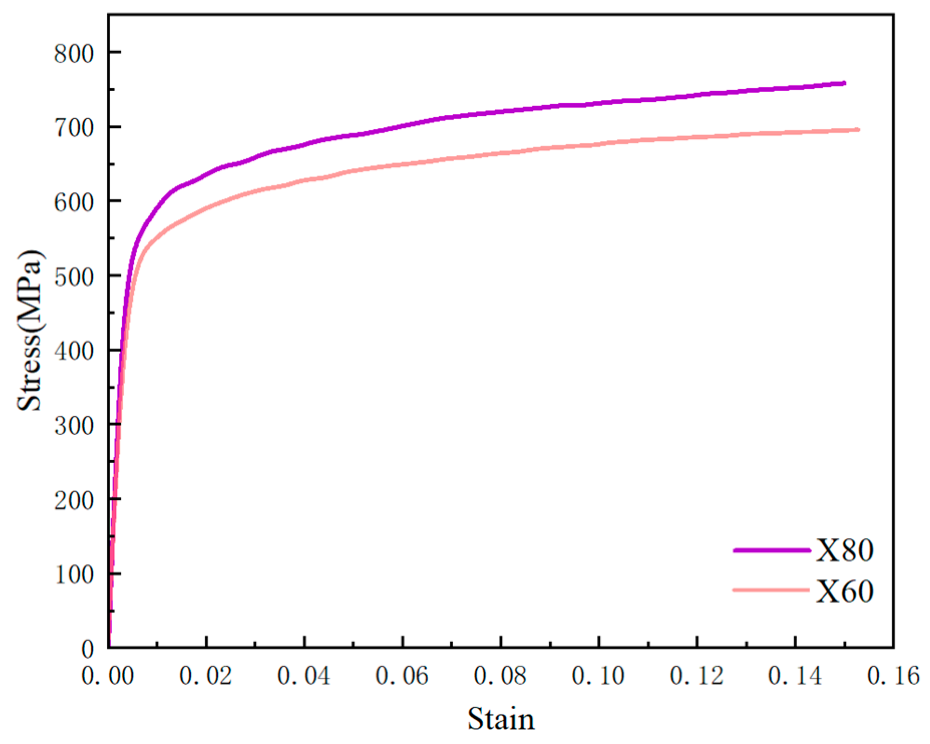
The Ramberg–Osgood constitutive model (Equation (1)) was adopted for the pipeline material [8]. Figure 3 shows the stress–strain curves for X60 and X80 pipeline steels; the corresponding material parameters are listed in

Table 2. Pipeline material parameters in the Ramberg–Osgood model.

Material	Density (kg/m3)	Elastic Modulus (MPa)	Poisson’s Ratio	Yield Strength (MPa)	$\mathit{\alpha }$	N
X60	7850	207,000	0.3	450	0.24	13
X80	7850	207,000	0.3	555	0.86	28

.

$$\epsilon ={\displaystyle \frac{{\sigma }_s}{E}}\left[{\displaystyle \frac{\sigma }{{\sigma }_s}}+\alpha {\left({\displaystyle \frac{\sigma }{{\sigma }_s}}\right)}^N\right]$$

(1)

Here, $\epsilon$ is the total strain, σ_s is the yield strength (MPa), E is the elastic modulus (MPa), and α and N are the Ramberg–Osgood parameters.

For sandy soil, the Mohr–Coulomb elastoplastic model was employed, which is suitable for simulating sand foundations where shear failure predominates. For clay, the Cap plasticity model was utilized [20]. This model is appropriate for simulating the volumetric compression and yielding behavior of normally consolidated clay under static loads. By introducing a “cap” yield surface to limit volumetric plastic deformation, it effectively reflects the hardening response and stress-path dependency of clay across a wide range of confining pressures. The soil domain is idealized as a homogeneous medium with uniform properties along the depth. This simplification is adopted for consistency with previous experimental and FE investigations [21] and to focus on the fault-induced PGD effect on pipeline response. The soil was assumed to be normally consolidated, and representative parameters are listed in

Table 3. Parameters were compiled/adopted from Refs. [20,21,22].

Soil Type	Density (kg/m3)	Elastic Modulus (MPa)	Poisson’s Ratio	Cohesion (kPa)	Friction Angle, φ (°)	Dilatancy Angle (°)	Void Ratio	Coefficient of Compressibility (MPa−1)	Stress Ratio
Sand	1550	33	0.27	5	30	0	---	---	---
Clay	1923	26	0.28	25	22	0	0.899	0.174	0.87

.

2.3. Boundary Conditions and Contact Settings

The model boundary conditions are shown in Figure 2. The bottom and adjacent side faces of the passive block were fixed, whereas prescribed displacements were applied to the active block to represent fault movement. The pipeline extends beyond the left boundary and was idealized as semi-infinite by applying a normal displacement constraint at the truncated end. The far-side wall of the passive block was also fixed. Coupling constraints were imposed on the centroid nodes at both pipe ends to enforce compatible deformation of the end sections.

A gravitational acceleration of 9.8 m/s² was applied to the entire model. A uniform internal pressure of 12 MPa was applied to the pipe inner surface, and an equivalent axial tensile stress of 1.57 MPa was applied at the right end. The soil was assumed to be fully saturated. Sand was modeled as drained, neglecting excess pore-water pressure, whereas clay was modeled as undrained, with undrained behavior represented by the cap-model parameters.

Surface-to-surface contact pairs were introduced to simulate pipe–soil interaction and relative block displacement. Tangential behavior was modeled using Coulomb friction (μ = 0.6 for pipe–soil contact and μ = 0.4 for soil–soil contact), and normal behavior was modeled as hard contact. The pipe surface and soil surface were assigned as leader and follower surfaces, respectively; at the fault plane, the hanging wall and footwall were set as leader and follower surfaces to represent inter-block slip.

2.4. Model Verification

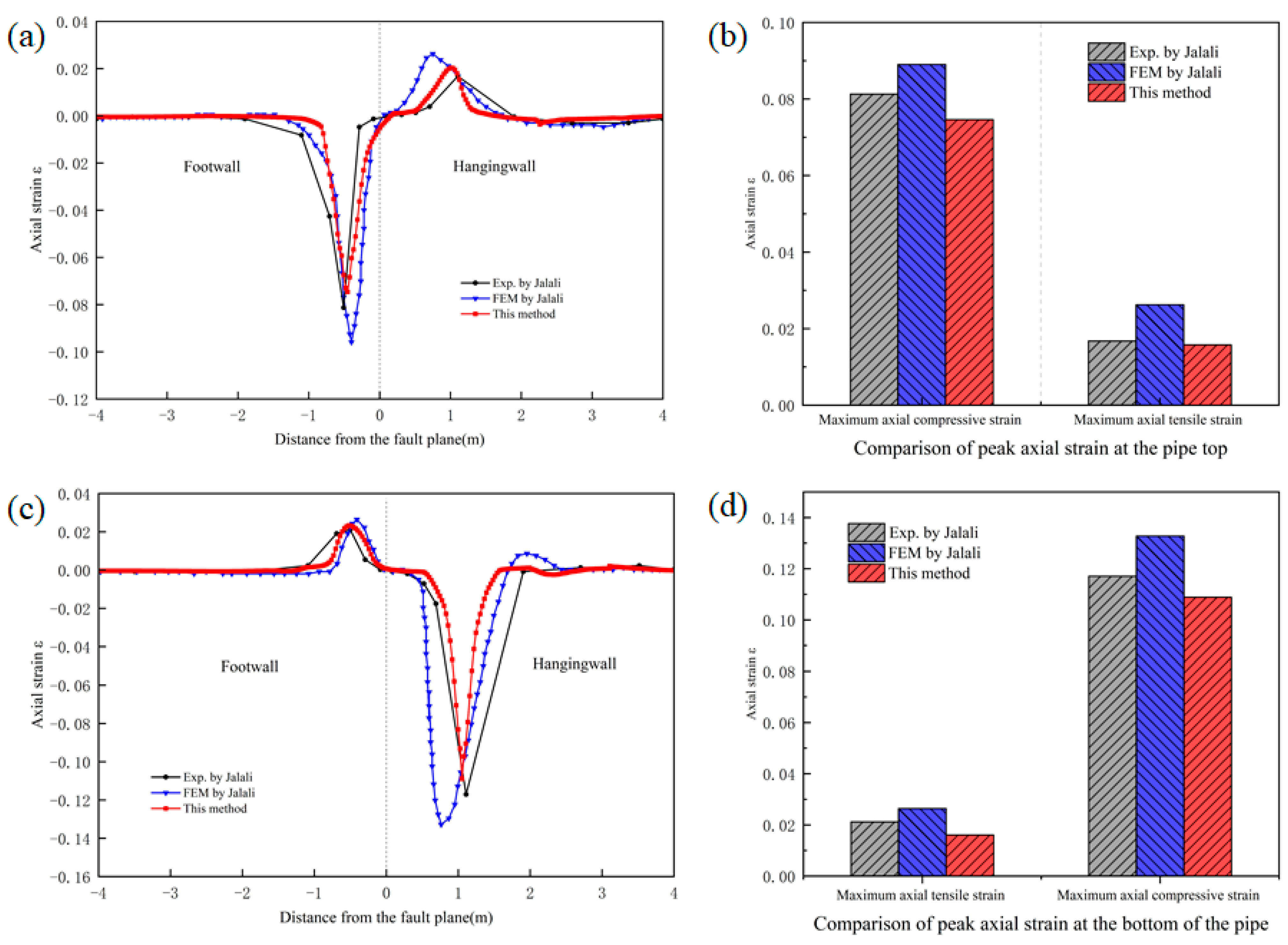
To verify the reliability of the established pipe–soil coupled model, a comparative analysis was conducted using experimental data published by Jalali et al. [8]. A pipe–soil coupled finite element model corresponding to the experimental apparatus was established based on the geometric dimensions, material parameters, and boundary conditions used in the test. The axial strain distributions at the pipe crown and invert were obtained and compared with the experimental and numerical results from the literature [21], as shown in Figure 4.

The results indicate that during the critical deformation stages before and after pipeline yielding, the simulated axial strain distributions are in good agreement with the experimental values, with some deviations observed only in regions of localized large deformation. Quantitatively, the relative errors in the peak compressive and tensile strains are 8.2% and 21.2% at the pipe crown and 7.0% and 10.1% at the pipe invert; all errors are ≤22%. Compared to the approach by Jalali et al. [21], this study utilizes C3D8R three-dimensional solid elements to simultaneously simulate both the pipeline and the surrounding soil. Normal and tangential tractions at the pipe–soil interface are transferred via 3D contact, enabling strains in multiple cross-sectional directions to be computed from a single stress field. This enables a more refined capture of localized buckling and the evolution of cross-sectional ovalization. In addition, an elastoplastic constitutive model calibrated to the tested pipe material was adopted to represent strain hardening at large strains, which improves predictive accuracy. Overall, the proposed pipe–soil coupled finite element model accurately predicts the mechanical response and deformation of buried pipelines subjected to fault movement, and it provides a basis for subsequent axial strain prediction and fragility analysis.

3. Mechanical Response Analysis of Buried Pipelines Under Faulting Modes

After completing the model verification, an X80 pipeline with an outer diameter of 0.864 m was selected as a case study to analyze the mechanical response under typical normal-slip and reverse-slip fault conditions. The fault dip angle was set to 45°, the crossing angle to 90°, and the burial depth to 4.5 m. The soil was sandy soil, and the dislocation displacements for normal-slip and reverse-slip faults were 3 m and 1 m, respectively.

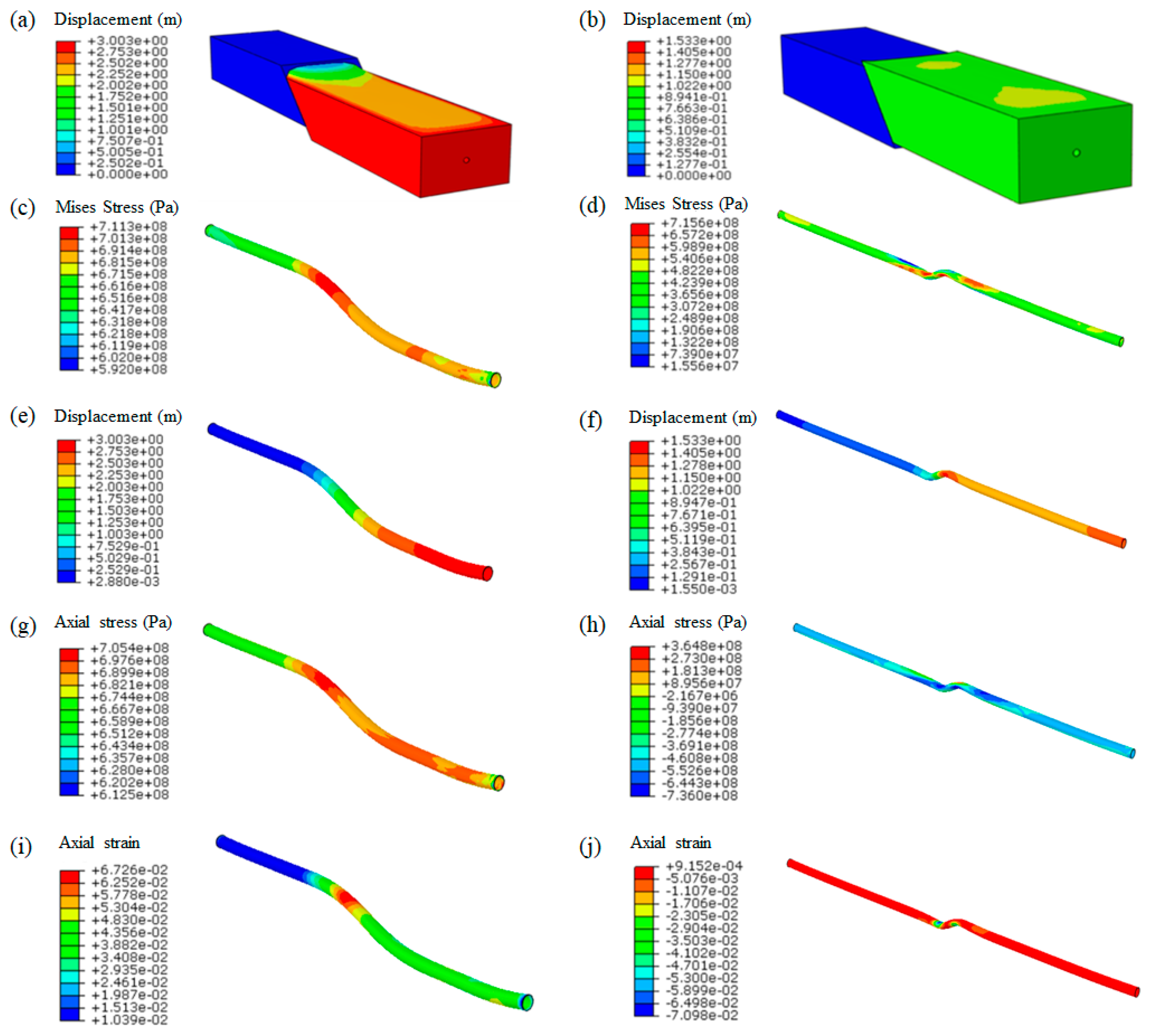
Figure 5 presents contour maps of pipeline deformation, von Mises stress, axial stress, and axial strain for the two fault-dislocation scenarios. Under normal-slip faulting, a pronounced bending zone develops near the fault, accompanied by a continuous offset of the pipe axis (Figure 5a,e). The maximum transverse displacement is close to 3 m. The high-displacement region extends more than 10 m on either side of the fault, indicating a broad influence zone. Under reverse-slip faulting (Figure 5b,f), pipe segments away from the fault remain nearly straight, and angular deformation is localized at the fault crossing. The maximum displacement is approximately 1 m and is mainly confined to a 3–5 m zone on either side of the fault, leading to severe local deformation.

The von Mises stress distributions (Figure 5c,d) are consistent with the deformation patterns described above. In the normal-slip case, a continuous high-stress band develops on the pipe outer wall near the fault, with a peak von Mises stress of approximately 711.3 MPa. The high-stress zone extends approximately ±10 m along the pipe axis, indicating yielding over an extended length. In the reverse-slip case, elevated von Mises stresses are largely confined to a 3–5 m region adjacent to the fault, with a peak of approximately 715.6 MPa and a steep local stress gradient. The axial stress distributions (Figure 5g,h) further show that, under normal-slip faulting, tensile stresses at both the crown and invert form a continuous axial tension zone. Under reverse-slip faulting, a pronounced compressive zone develops at the invert, whereas compression at the crown is relatively small. This suggests that reverse faulting is governed by localized axial compression coupled with bending [23].

The axial strain distributions (Figure 5i,j) provide a direct indicator of potential failure risk. In the normal-slip case, axial tensile strain increases markedly in the pipe segment near the fault, reaching a maximum of approximately 6%. In the reverse-slip case, pronounced compressive strain develops at the invert near the fault, with values of −6% to −7%. These strains are highly localized within a 3–5 m zone on either side of the fault, whereas axial strain far from the fault is close to zero. Although the deformation patterns differ between the two fault modes, severe axial strain localization occurs near the fault in both cases [21]. This localization is a primary factor governing pipeline failure.

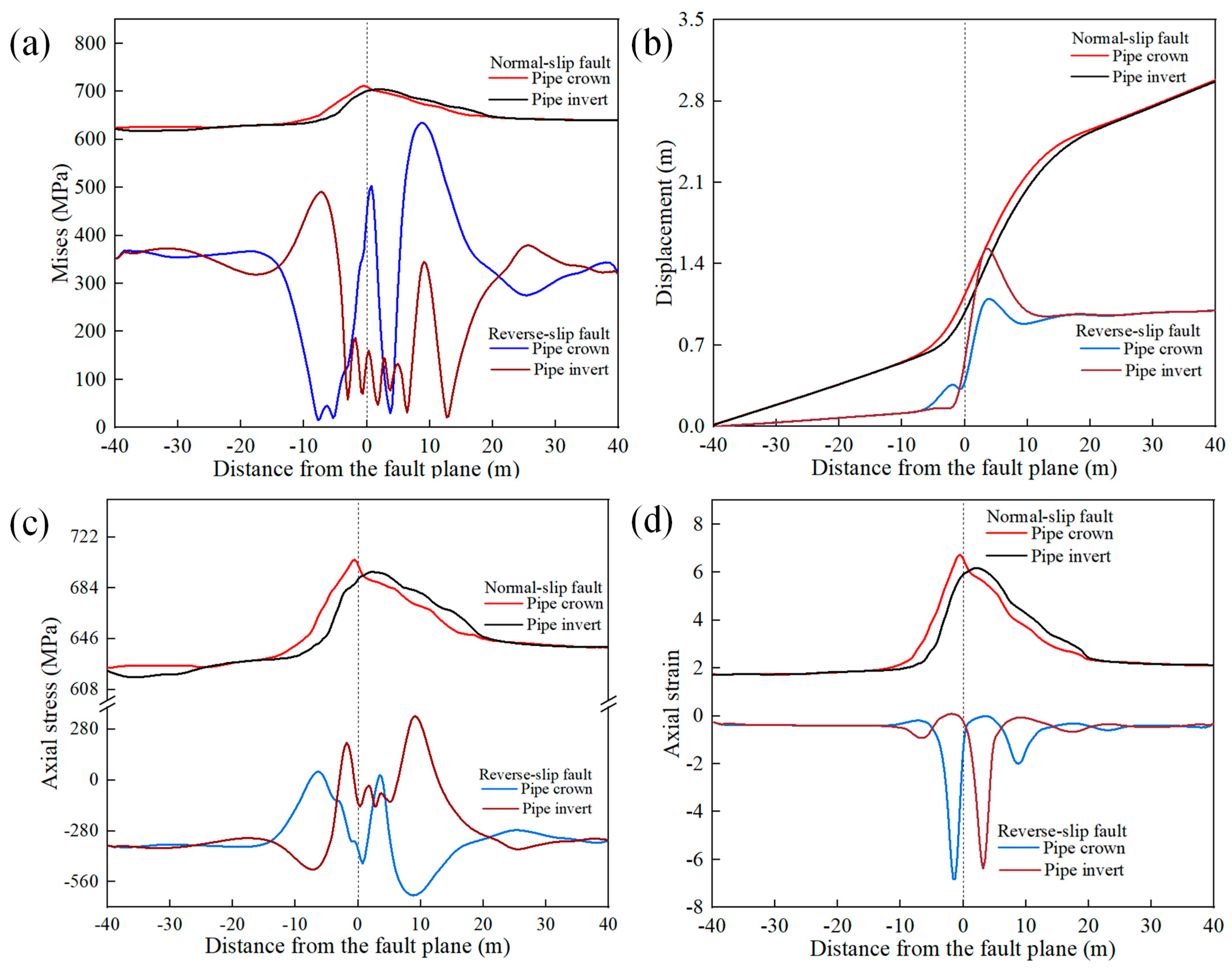
Figure 6 shows the axial distributions of von Mises stress, displacement, axial stress, and axial strain at the pipe crown and invert for both faulting scenarios. The displacement profiles (Figure 6b) show that, under normal-slip faulting, the axial displacements at the crown and invert nearly coincide. Displacement increases gradually from near zero at the far end of the passive block to a plateau of approximately 3 m on the active-block side, consistent with the imposed fault offset. In contrast, under reverse-slip faulting, axial displacement peaks near the fault and is mainly confined to the 0–5 m region on the active-block side. Displacement in the remaining segments is nearly constant, indicating a more localized deformation influence zone.

The von Mises stress distribution (Figure 6a) shows that under the normal-slip condition, the stress exhibits a “plateau-type” distribution along the axis, with values around 600 MPa far from the fault, rising to approximately 700 MPa near the fault, and maintaining high levels within about 10 m on both sides. Under reverse-slip faulting, high von Mises stress occurs only as several sharp peaks on either side of the fault. The axial stress curves (Figure 6c) show a similar pattern: under normal-slip, a high tensile stress zone approximately 20 m wide forms near the fault; under reverse-slip, the stress fluctuates sharply near the fault and decays rapidly further away.

The axial strain distribution (Figure 6d) reveals that under normal-slip faulting, the axial tensile strains at both the pipe crown and invert exceed 4% over a large range adjacent to the fault, with a peak of about 6%. These values are substantially higher than the strain limits typically adopted in conventional design (≈2–3%), and the high-strain zone extends for more than 10 m. In the reverse-slip case, axial compressive strain at the invert peaks at nearly −7% near the fault, whereas strain elsewhere remains close to zero. This indicates that failure risk is highly concentrated in the immediate fault-crossing region. Compared with stress, both the exceedance of axial strain beyond the limit and the axial extent of the high-strain region provide more direct indicators of potential damage severity [5]. Therefore, pipeline failure under slip faulting should be assessed primarily by whether axial strain exceeds prescribed limits [17].

4. Prediction Model for Peak Axial Strain of Buried Pipelines Under Faulting Modes

4.1. Applicability of the Peak Strain Prediction Model

Based on the analysis in Section 3, this study adopts the limit strain (${\epsilon }_{\mathrm{crit}}$) as the criterion for pipeline failure [7,8], as shown in Equations (2) and (3):

$${\epsilon }_{\mathrm{crit}}=0.5\left({\displaystyle \frac{t}{D}}\right)-0.0025+3000{({\displaystyle \frac{{\sigma }_h}{E}})}^2$$

(2)

$${\sigma }_h=\left\{\begin{array}{l}{\displaystyle \frac{pD}{2t}},\hspace{1em}{\displaystyle \frac{pD}{2t{\sigma }_s}}\le 0.4\\ 0.4{\sigma }_s,\hspace{1em}{\displaystyle \frac{pD}{2t{\sigma }_s}}>0.4\end{array}\right.$$

(3)

where ${\sigma }_h$ is the hoop stress (MPa), p is the internal pipeline pressure (MPa), and ${\sigma }_s$ is the yield strength (MPa). The hoop stress is defined as ${\sigma }_h$ = pD/2t.

4.2. Prediction Model for Peak Axial Strain

The peak compressive strain of a pipe can be assumed to be a function of all influence parameters (Equation (4)). Based on the finite element analysis results and with reference to existing studies [7,13], reasonable independent dimensionless parameters were further selected to conduct the parametric analysis, which transforms Equation (4) into Equation (5). For specific parameter definitions, see the notes below the equations. From 352 finite element simulations, data screening was performed according to the criterion that axial strain must be less than ${\epsilon }_{\mathrm{crit}}$, resulting in 208 sets of valid peak strain data. And, the functional relationships with strain demand can be assumed to form the assumed equations (Equations (6) and (7)). Non-linear regression analysis was applied to this dataset to establish prediction models for the peak axial strain of pipelines under normal-slip and reverse-slip faulting. The range of pipeline and fault parameters used in the models is provided in

Table 4. Parameter range.

Parameter	Range
Crossing angle β/°	90°
Dip angle ψ/°	45–90°
Pipeline material	X60, X80
Soil type	Sand, Clay
Diameter D(thickness t)/mm	406–864 mm
Buried depth H/m	1 m−4.5 m
Displacement of the normal-slip fault	0–1.5 m
Displacement of the reverse-slip fault	0–0.45 m

.

$$\epsilon =f({\delta }_s,\psi ,D,t,p,{\sigma }_s,F_{Axial},F_{Up},F_{Bearing},F_{Axial})$$

(4)

$$\epsilon =f({\displaystyle \frac{{\delta }_s{F}_{Axial}}{{\sigma }_s}},{\displaystyle \frac{\psi \pi }{180}},{\displaystyle \frac{D}{t}},{\displaystyle \frac{D}{{\delta }_s}},{\displaystyle \frac{p}{{\sigma }_s}},{\displaystyle \frac{F_{Up}{D}^3}{EI}},{\displaystyle \frac{F_{Bearing}{D}^3}{EI}},{\displaystyle \frac{F_{Axial}D}{EA}})$$

(5)

$$\begin{array}{l}{\epsilon }_N=c_1{\left({\displaystyle \frac{{\delta }_s{F}_{Axial}}{{\sigma }_s}}\right)}^{\left(c_{14}{\left({\displaystyle \frac{\psi \pi }{180}}\right)}^2+c_2{\displaystyle \frac{\psi \pi }{180}}+c_3+c_4{\displaystyle \frac{p}{{\sigma }_s}}\right)}\left(\tanh {\displaystyle \frac{c_5\psi }{90}}+c_6\right){\left({\displaystyle \frac{F_{Up}{D}^3}{EI}}\right)}^{c_7}\\ {\left({\displaystyle \frac{F_{Bearing}{D}^3}{EI}}\right)}^{c_8}{\left({\displaystyle \frac{F_{Axial}D}{EA}}\right)}^{c_9}{\left({\displaystyle \frac{D}{{\delta }_s}}\right)}^{c_{10}}{\left({\displaystyle \frac{D}{t}}\right)}^{c_{11}}\left({\left({\displaystyle \frac{p}{{\sigma }_s}}\right)}^{c_{12}}+c_{13}\right)+c_{15}\end{array}$$

(6)

$$\begin{array}{l}{\epsilon }_R=d_1{\left({\displaystyle \frac{{\delta }_s{F}_{Axial}}{{\sigma }_s}}\right)}^{\left(-{\left(\pi \psi /180-1/4\pi \right)}^2+d_2\pi \psi /180+d_3+d_4\left({\displaystyle \frac{p}{{\sigma }_{\mathrm{s}}}}\right)\right)}\left({\left(\pi \psi /180-1/4\pi \right)}^2+d_5\right)\\ {\left({\displaystyle \frac{F_{Up}{D}^3}{EI}}\right)}^{d_6}{\left({\displaystyle \frac{F_{Bearing}D}{EA}}\right)}^{d_7}{\left({\displaystyle \frac{F_{Axial}D}{EA}}\right)}^{d_8}{\left({\displaystyle \frac{D}{{\delta }_s}}\right)}^{d_9}{\left({\displaystyle \frac{D}{t}}\right)}^{d_{10}}\left({\left({\displaystyle \frac{p}{{\sigma }_s}}\right)}^{d_{11}}+d_{12}\right)+d_{13}\end{array}$$

(7)

$$F_{Axial}=\pi D\alpha c+\pi DH\overline{\gamma }{\displaystyle \frac{2-\sin \varphi }{2}}\tan (f\varphi )$$

(8)

$$F_{Up}=u_{1}cD+u_2\overline{\gamma }HD$$

(9)

$$F_{Bearing}=t_{1}cD+t_2\overline{\gamma }HD+t_3\overline{\gamma }{\displaystyle \frac{D^2}{2}}$$

(10)

$$\alpha =0.608-0.123c-0.274/(c^2+1)+0.695/(c^3+1)$$

(11)

$$t_1=\left[\cot (\varphi +0.001)\right]\left[e^{\pi \tan (\varphi +0.001)}{\tan }^2\left(45+{\displaystyle \frac{\varphi +0.001}{2}}\right)-1\right]$$

(12)

$$t_2=e^{\pi \tan \varphi }{\tan }^2\left(45+{\displaystyle \frac{\varphi }{2}}\right)$$

(13)

$$t_3=e^{(0.18\varphi -2.5)}$$

(14)

Here, ${\epsilon }_N$ and ${\epsilon }_R$ are the peak axial strains for normal-slip and reverse-slip faulting, respectively. ${\delta }_s$ is the fault displacement (m); p is the internal pressure of the pipeline (MPa); ${\sigma }_s$ is the yield strength (MPa). I is the moment of inertia (m⁴₎; A is the cross-sectional area of the pipeline (m²). $F_{Axial}$ is the axial force (kN/m); $F_{Up}$ and $F_{Bearing}$ are the vertical uplift force and vertical bearing force (kN/m), respectively; $\overline{\gamma }$ is the effective unit weight of the soil (N/m³); f is the friction coefficient; α is the adhesion coefficient. u₁ and u₂ are the vertical uplift coefficients; t₁, t₂ and t₃ are the vertical compression coefficients for clayey soil. The non-linear regression parameters for the normal-slip fault mode (c₁–c₁₅) and the reverse-slip fault model (d₁–d₁₃) are defined as shown in Equations (15) and (16), respectively.

$$\left(\begin{array}{cccc}{c}_1=0.7003& c_2=-0.0263& c_3=1.4279& c_4=-0.3980\\ c_5=0.5226& c_6=-0.8338& c_7=0.7209& c_8=-0.001\\ c_9=-0.6249& c_{10}=0.6813& c_{11}=-0.8614& c_{12}=-0.1000\\ c_{13}=0.1899& c_{14}=0.3028& c_{15}=-0.0004\end{array}\right)$$

(15)

$$\left(\begin{array}{cccc}{d}_1=-0.1283& d_2=0.4473& d_3=5.0062& d_4=-3.6804\\ d_5=2.4450& d_6=0.0347& d_7=-0.3529& d_8=3.8185\\ d_9=3.3435& d_{10}=1.4652& d_{11}=-3.8481& d_{12}=5.2398\\ d_{13}=-0.0004\end{array}\right)$$

(16)

Existing regression or semi-empirical strain-demand equations for fault-crossing pipelines are often developed for specific fault kinematics and modeling assumptions. For example, Liu et al. [7]. reported regression-based strain demand models for X80 pipelines crossing reverse or oblique-reverse faults, where pipe–soil interaction is represented through spring-based idealizations and the formulation is intended to support strain-based design calculations [13]. Such studies demonstrate the practical value of explicit prediction relationships, while their use is commonly tied to the adopted interaction idealization, targeted fault components, and the parameter ranges considered. In the present study, the peak axial strain prediction equations are derived from a validated three-dimensional pipe–soil coupled finite element model that captures large deformation, nonlinear contact and frictional interaction, and material nonlinearity under normal-slip and reverse-slip faulting. To reflect the different response mechanisms in these two faulting modes, separate functional forms are established for normal-slip and reverse-slip conditions. The equations further incorporate fault displacement together with key geometric, material, and soil-related parameters (e.g., burial depth, soil type, pipe diameter, and steel grade) based on the dedicated FE database and screened strain data employed in this work. In addition, the present closed-form equations are complementary to recent computationally efficient response-prediction routes, such as the finite-difference-based strain tool integrated with Monte Carlo simulation for probabilistic analysis reported by Zheng et al. and the PINN-based surrogate and reliability-analysis frameworks (PINN-RA) proposed by Taraghi et al., which couple a PINN surrogate with Monte Carlo simulation to reduce repeated numerical evaluations in reliability assessment [9,10,11]. Compared with these approaches, the explicit regression form adopted herein provides a transparent demand model that can be directly embedded into the subsequent fragility framework for rapid generation of fragility curves across parameter combinations, without additional finite element analyses. These demand models can be embedded into the subsequent fragility assessment framework using fault displacement as the intensity measure, enabling rapid generation of fragility curves for different parameter combinations without additional finite element analyses.

4.3. Verification of the Peak Axial Strain Prediction Model

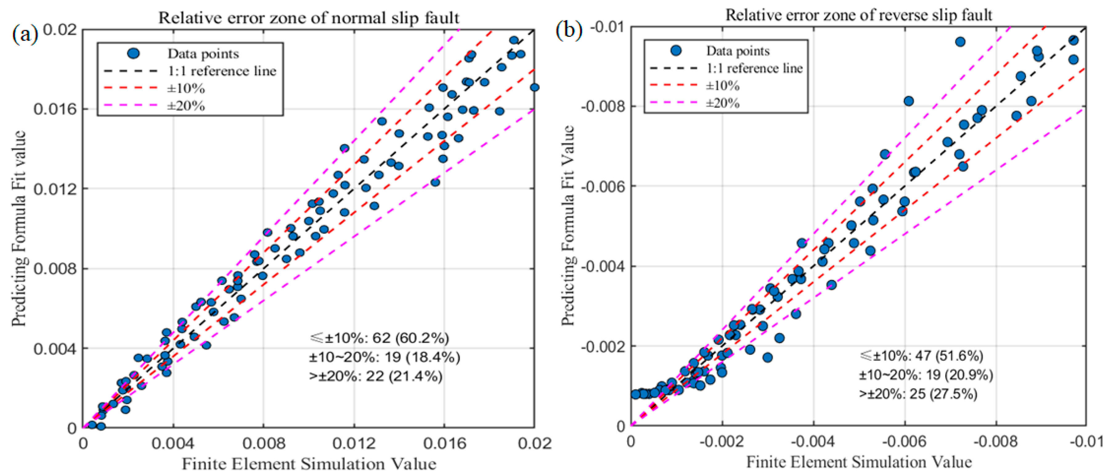
Figure 7 compares the model predictions with finite element results for both normal-slip and reverse-slip faulting cases. Most data points lie close to the 45° line, indicating good agreement between the predictions and the simulations. For normal slip, 60.2% of points have errors <10%, and 78.6% have errors <20%. For reverse slip, 51.6% of points have errors <10%, and 72.5% fall within a 20% error margin. Overall, the proposed models provide accurate and reliable predictions of peak axial strain under representative slip-faulting conditions.

To evaluate the generalization capability of the model, several independent validation cases were selected. For each case, the fault displacement was substituted into Equations (4) and (5) to compute the predicted strain, and the prediction error was quantified using the metric defined in Equation (17). If the prediction error is lower than the uncertainty level implied by the regression residuals, the model is considered to exhibit no substantial overfitting. The validation results satisfy this criterion for all test cases, indicating that the proposed models generalize well within the specified parameter range [4,5] and are applicable to a broad set of engineering scenarios.

$$MS{E}_{valid}={\displaystyle \frac{1}{n}}{\displaystyle \sum _{i=1}^n\left({{\epsilon }_{pred}}^2-{\epsilon }^2\right)}$$

(17)

5. Fragility Analysis of Buried Pipelines Under Slip Faulting

5.1. Fragility Assessment Methodology

The fragility [24] of a buried pipeline subjected to fault displacement can be defined as the conditional probability that the structural demand D exceeds a specific capacity or damage state C for a given intensity measure IM = x, as expressed in Equations (18)–(21):

$$F(x)=P\left[D\ge C | IM=x\right]$$

(18)

$$D=m_{EDP|IM}·{\eta }_{EDP|IM}$$

(19)

$$C=m_C{\eta }_C$$

(20)

$$m_C={\displaystyle \frac{{\mu }_C}{\sqrt{1+{\delta }_C^2}}}$$

(21)

where F(x) is the pipeline fragility function; $m_{EDP|IM}$ is the median strain response under different fault displacements; ${\eta }_{EDP|IM}$ is the random error following a lognormal distribution with a median of 1 and a lognormal standard deviation of ${\beta }_{EDP|IM}$ [25]; $m_C$ represents the critical strain response for different damage states; ${\eta }_C$ is the random error following a lognormal distribution with a median of 1 and a lognormal standard deviation of ${\beta }_C$; ${\mu }_C$ and ${\delta }_C$ are the mean value and coefficient of variation of the limit strain for various damage states, respectively.

In conventional pipeline fragility analysis, fragility curves are typically represented by a lognormal cumulative distribution function, shown in Equation (22). In this study, the total dispersion $\beta$ accounts for three contributions: demand uncertainty (${\beta }_{EDP|IM}$), capacity uncertainty (${\beta }_C$), and modeling uncertainty (${\beta }_M$) [26]. The demand uncertainty [25] represents the scatter of the strain-demand prediction relative to the FE results and is quantified from the residuals of the regression-based demand models developed in Section 4 (i.e., the logarithmic error between predicted and simulated peak axial strains). This is consistent with the notion that the demand model serves as a surrogate of FE response and its residuals should be propagated into fragility analysis. The capacity uncertainty reflects the variability of limit strains due to material properties, manufacturing tolerances, welding/defect conditions, and other capacity-related factors. ${\beta }_C$ is taken as 0.25 [27,28]. The modeling uncertainty represents the epistemic uncertainty associated with modeling idealizations (e.g., constitutive assumptions, contact/friction representation, and boundary idealization) and is taken as 0.2 following [27]. Considering the total dispersion ($\beta$) [26], the fragility function for pipelines in fault zones is derived as shown in Equations (23)–(25):

$$F(x)=\mathsf{\Phi }\left[{\displaystyle \frac{\ln x-\ln m_c)}{\beta }}\right]$$

(22)

$$F(x)=\mathsf{\Phi }\left[{\displaystyle \frac{\ln (m_{EDP|IM})-\ln (m_C)}{\beta }}\right]$$

(23)

$${\beta }_{EDP|IM}=\sqrt{{\left[\ln (D)-\ln (m_{EDP|IM})\right]}^2}$$

(24)

$${\beta }_C=\sqrt{\ln (1+{\delta }_C^2)}$$

(25)

$$\beta =\sqrt{{\beta }_{EDP|IM}^2+{\beta }_C^2+{\beta }_M^2}$$

(26)

where $\mathsf{\Phi }\left[·\right]$ is the standard normal cumulative distribution function; $\beta$ is the total lognormal standard deviation; ${\beta }_{EDP|IM}$ represents the uncertainty between calculated and predicted values; ${\beta }_C$ represents the uncertainty in structural capacity; ${\beta }_M$ reflects the uncertainty in structural modeling accuracy.

Traditional least squares-based fragility analysis requires numerous finite element simulations for each parameter combination to calibrate the median demand and dispersion [25], which limits extrapolation beyond the available dataset. Here, the peak axial strain prediction models (Equations (6) and (7)) are embedded directly into the fragility function. Using the peak axial strain computed from these equations as the demand input, fragility curves can be rapidly constructed for any parameter combination without additional finite element analyses, thereby substantially improving assessment efficiency.

To quantify pipeline damage under fault displacement, damage states must first be classified. Following Shinozuka et al. [29], pipeline damage is categorized into three states: basic intact, moderate damage, and severe damage. Table 5 provides the criteria for each limit state and the corresponding critical axial strains (${\epsilon }_y$ and $0.7{\epsilon }_y$). Substituting these critical strains into Equation (19) and using Equation (22) yields the corresponding fragility curves. A damage probability matrix is then constructed using Equation (27).

Table 5. Classification of limit damage states for buried pipelines.

Damage State	Performance Description	Strain Criterion
Basic intact	Slight deformation without rupture or leakage.	${\epsilon }_p<0.7{\epsilon }_y$
Moderate damage	Significant deformation or buckling, potential minor rupture or leakage; repairs are required for normal operation.	$0.7{\epsilon }_y<{\epsilon }_p<{\epsilon }_y$
Severe damage	Pipeline rupture or massive leakage; the pipeline must be replaced.	${\epsilon }_p>{\epsilon }_y$

Table 5. Classification of limit damage states for buried pipelines.

Damage State	Performance Description	Strain Criterion
Basic intact	Slight deformation without rupture or leakage.	${\epsilon }_p<0.7{\epsilon }_y$
Moderate damage	Significant deformation or buckling, potential minor rupture or leakage; repairs are required for normal operation.	$0.7{\epsilon }_y<{\epsilon }_p<{\epsilon }_y$
Severe damage	Pipeline rupture or massive leakage; the pipeline must be replaced.	${\epsilon }_p>{\epsilon }_y$

$$\left\{\begin{array}{l}{P}_{int}=1-P_{leak}\\ P_{med}=P_{leak}-P_{break}\\ P_{sev}=P_{break}\end{array}\right.$$

(27)

Here, $P_{leak}$ and $P_{break}$ denote the probabilities of the slight-damage and moderate-damage limit states, respectively, while $P_{int}$, $P_{med}$, and $P_{sev}$ are the probabilities of being intact, moderately damaged, and severely damaged, respectively.

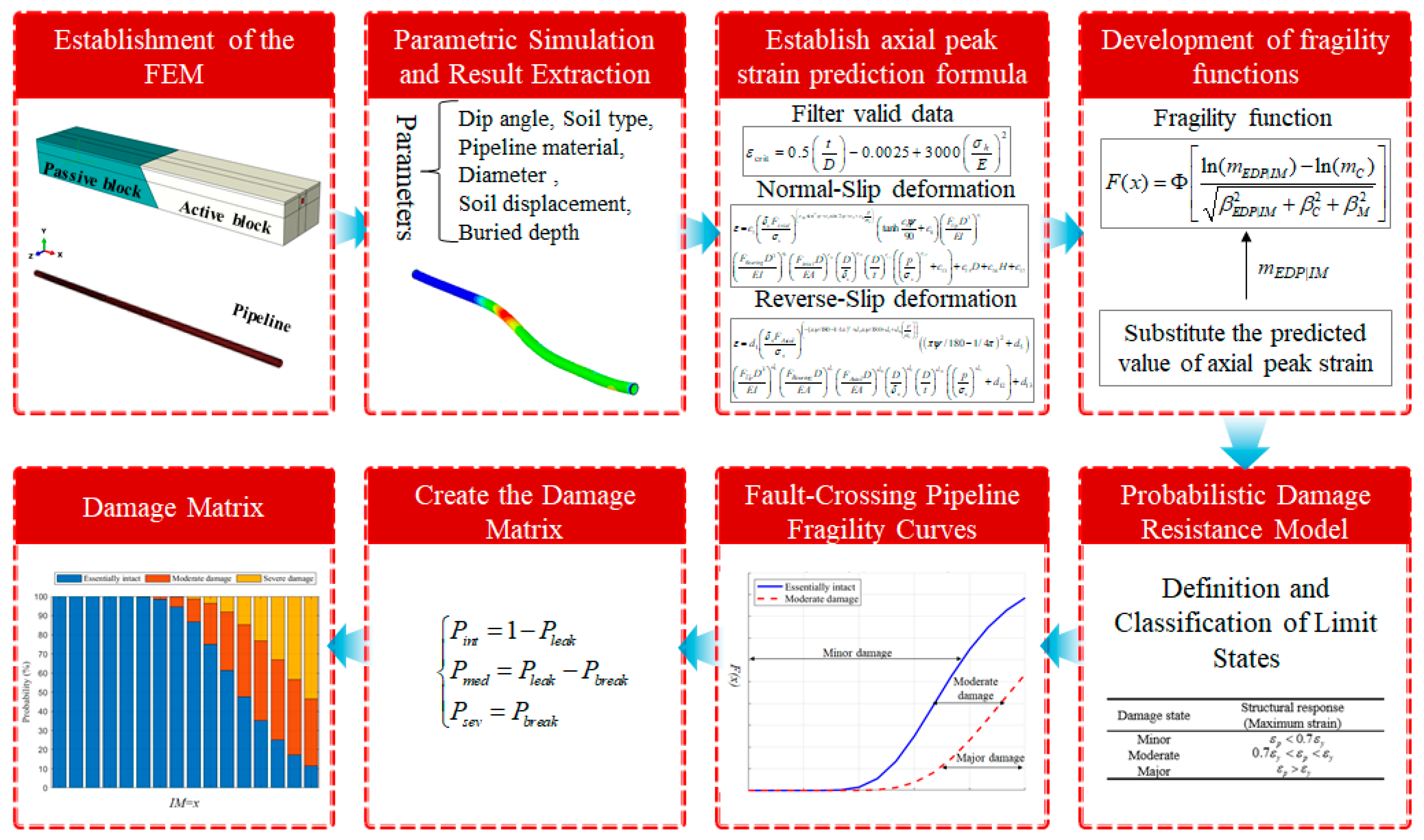
The proposed procedure for fragility assessment of buried pipelines subjected to slip faulting is summarized in Figure 8 and includes the following steps.

Step 1: Develop a 3D pipe–soil coupled finite element model and verify and calibrate it.

Step 2: Perform parametric simulations to obtain peak axial strain for combinations of fault dip angle, soil type, pipe grade, pipe diameter, fault displacement, and burial depth.

Step 3: Screen the dataset and develop regression-based models to predict peak axial strain (Equations (6) and (7)).

Step 4: Construct the fragility function with fault displacement as the intensity measure (Equation (23)) using the predicted peak axial strain as the demand input.

Step 5: Define damage limit states and specify the corresponding critical strains based on Table 5.

Step 6: Compute the exceedance probability for each damage state at different fault displacements and plot the fragility curves.

Step 7: Construct the damage probability matrix using Equation (27) to complete the fragility assessment of the fault–pipeline system.

5.2. Analysis of Fault-Pipeline Fragility Assessment Results

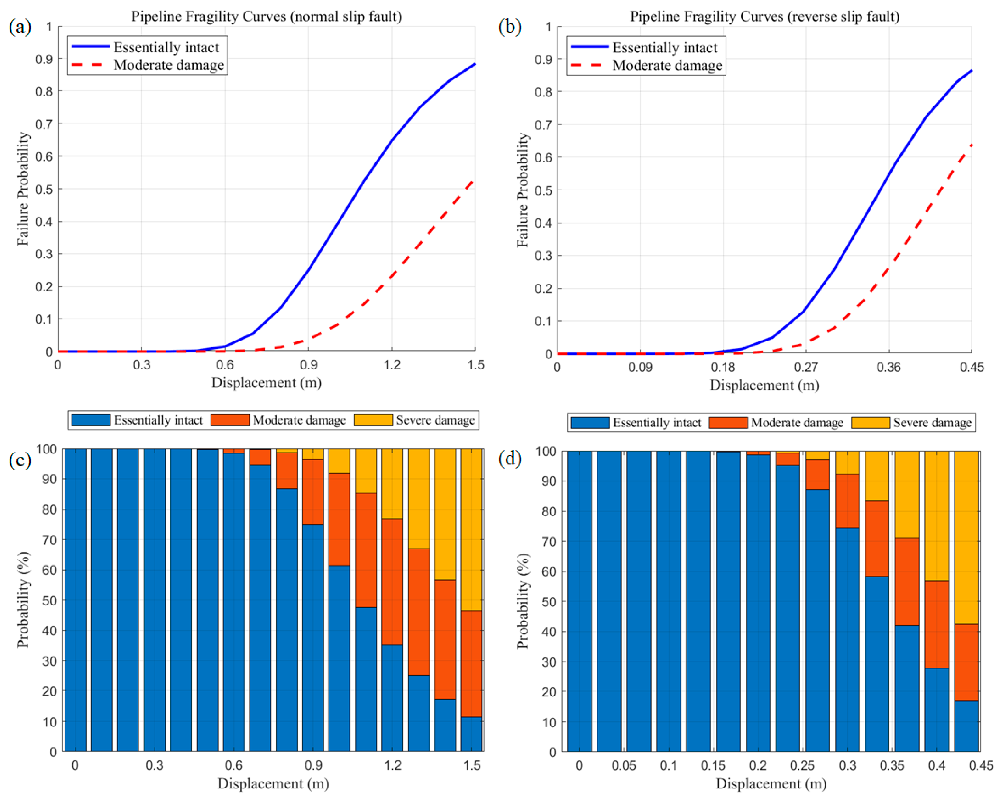
Using the methodology described above, the fragility curves and damage probability matrices for the two fault conditions discussed in Section 3 were obtained, as shown in Figure 9. In Figure 9a,b, the blue curve denotes the threshold for the basic intact state; for a given fault displacement, the area above this curve corresponds to the probability that the pipeline remains intact. The red curve denotes the threshold for moderate damage; the area below it corresponds to the probability of severe damage, whereas the area between the blue and red curves corresponds to the probability of moderate damage.

As shown in Figure 9c, when fault slip is <0.6 m, the probability of the pipeline remaining in the basic intact state is nearly 100%. At a slip of 1.2 m, the probability of basic intact decreases to 35.05%, whereas moderate damage and severe damage increase to 41.86% and 23.09%, respectively. Therefore, 0.6 m is taken as the displacement threshold for the transition from intact to damaged states under normal-slip faulting [30]. Figure 9d shows that, under reverse-slip faulting, the basic intact probability is 100% for slip <0.2 m. At a slip of 0.4 m, the basic intact probability decreases to 27.78%, with moderate damage at 43.21% and severe damage at 29.01%. Notably, the intact-to-damage displacement threshold under normal-slip faulting is about three times that under reverse-slip faulting, indicating a substantially higher damage risk for reverse-slip events.

At small fault slip, stresses and deformations are minimal and the pipeline remains elastic, corresponding to an intact probability of 100%. As slip increases, axial strain intensifies and the pipeline transitions from elastic behavior to yielding, increasing failure risk. Normal-slip faulting is dominated by axial tension and bending, whereas reverse-slip faulting is dominated by axial compression and bending. With increasing fault displacement, accumulating axial plastic deformation substantially increases the probability of pipeline damage [31,32,33].

5.3. Influence of Key Parameters on Pipeline Fragility

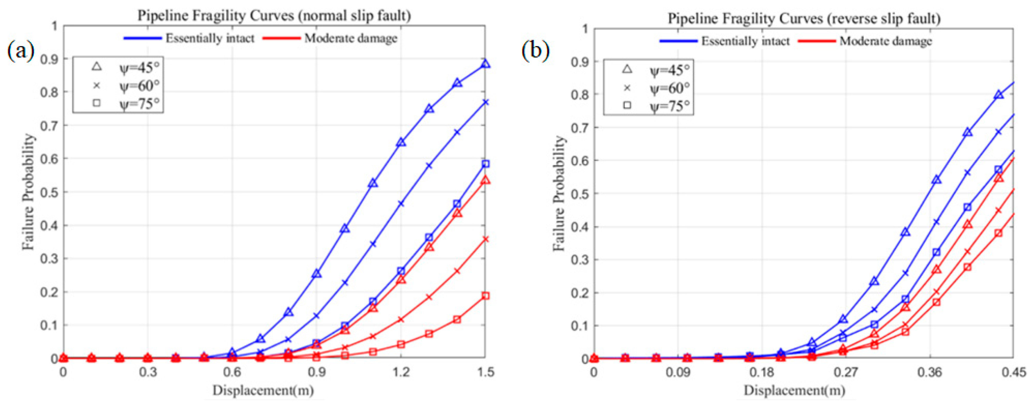
Figure 10, Figure 11, Figure 12, Figure 13 and Figure 14 present fragility curves for three fault dip angles (45°, 60°, and 75°), two pipe grades (X60 and X80), two soil types (sand and clay), three outer diameters (406, 610, and 864 mm), and three burial depths (1.0, 2.0, and 4.5 m). Figure 10 shows that, for both normal-slip and reverse-slip faulting, the failure probability increases as dip angle decreases from 75° to 45° at a given fault displacement. In addition, the displacement threshold for damage initiation is higher for normal-slip faulting than for reverse-slip faulting. Consequently, as fault displacement increases, pipelines subjected to reverse-slip faulting exhibit higher failure probabilities than those subjected to normal-slip faulting [31,34]. For both faulting modes, a smaller dip angle promotes greater accumulation of slip-induced axial deformation, thereby increasing the probability of pipeline damage.

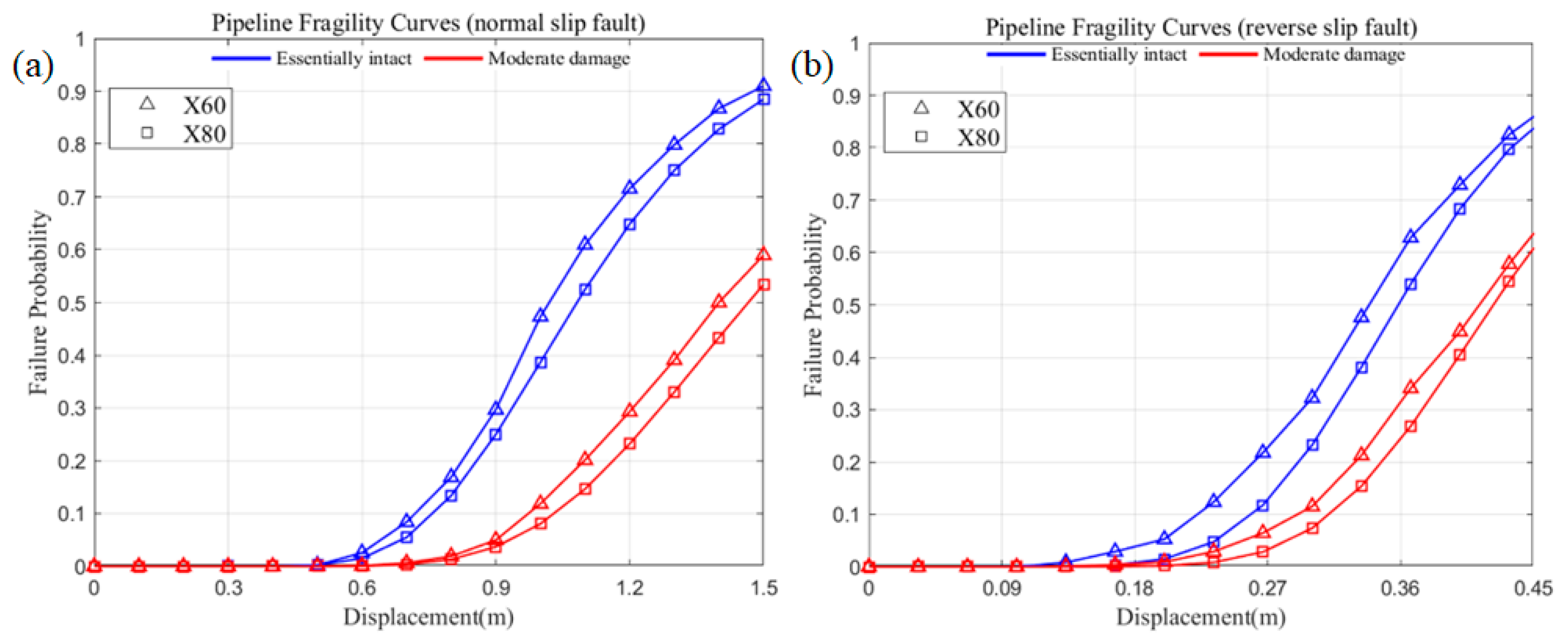
Figure 11 shows that, as fault displacement increases, failure probabilities for both X60 and X80 pipelines increase from near zero under both faulting modes. At a given displacement, X60 pipelines exhibit substantially higher failure probabilities than X80 pipelines under both faulting modes. Therefore, under both normal-slip and reverse-slip faulting, higher-strength steel pipelines provide a larger displacement margin and lower failure probability [35].

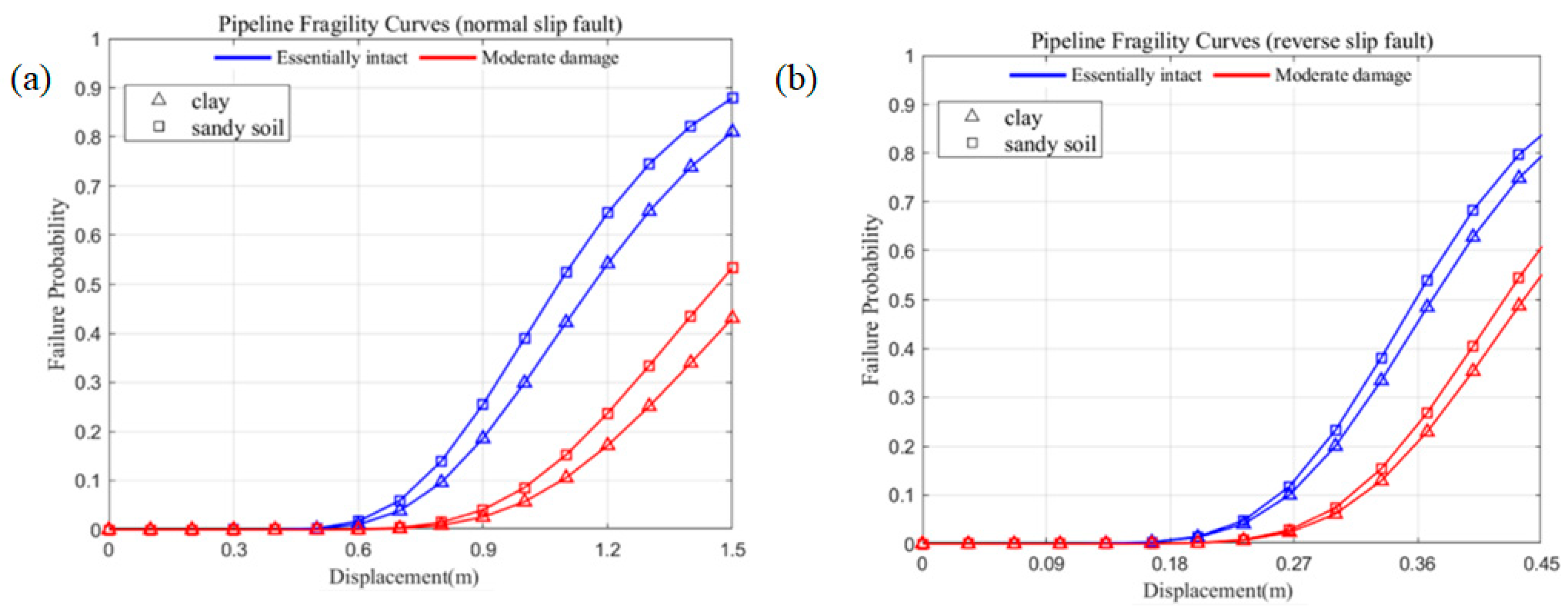
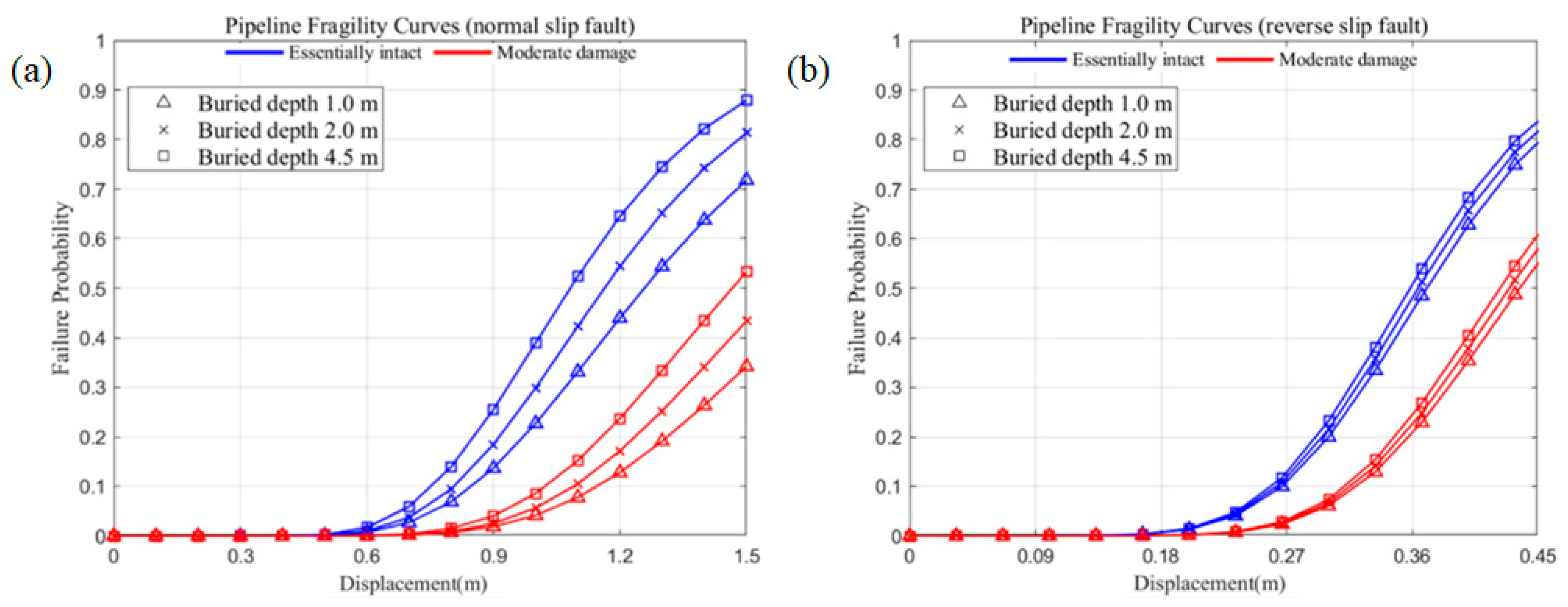
Figure 12 presents fragility curves for pipelines in sandy and clayey soils. In all cases, failure probability increases with fault displacement. Under both slip-faulting modes, the probabilities of moderate and severe damage are higher for pipelines in sandy soil than for those in clayey soil. Therefore, within the parameter range considered, pipelines in sandy soil exhibit higher failure probabilities than those in clayey soil at the same slip mode and displacement [35,36]. This difference is attributed to the higher elastic modulus and internal friction angle of sandy soil relative to clay (Table 3). Under the same confining pressure, sandy soil provides stronger lateral confinement and higher pipe–soil interface friction. As a result, fault-induced displacement is transferred to the pipeline over a shorter axial length, amplifying local tensile, compressive, and bending strains. In contrast, clay has a larger compression index and greater volumetric compressibility, allowing it to accommodate part of the fault displacement through volumetric plastic deformation during loading and thereby buffer pipeline deformation. Consequently, failure probability is lower in clay for the same displacement.

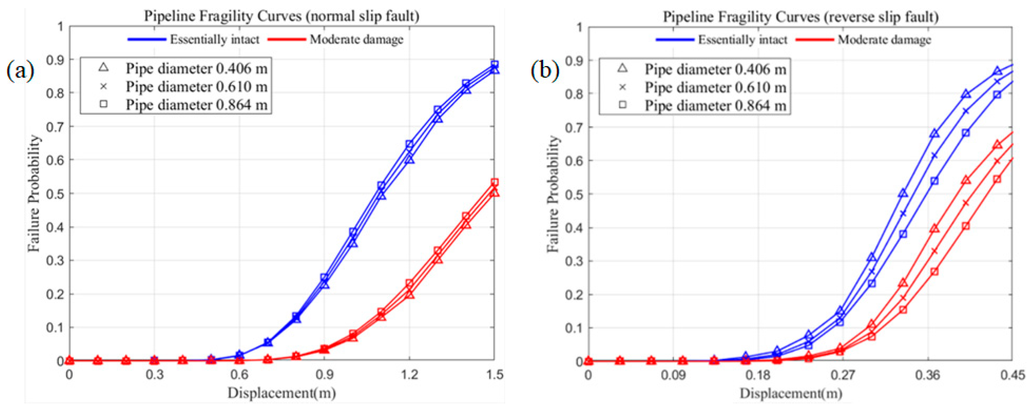
Figure 13 shows that the fragility curves for the three pipe diameters nearly overlap at small displacements (normal slip: d < 1.2 m; reverse slip: d < 0.3 m). As slip displacement increases, failure probability rises rapidly under both faulting modes. For normal-slip faulting, pipe diameter has a negligible effect on failure probability, and the fragility curves almost coincide. In contrast, under reverse-slip faulting, smaller-diameter pipelines exhibit higher failure probabilities than larger-diameter pipelines.

Figure 14 indicates that, for both normal-slip and reverse-slip faulting, pipelines at all three burial depths show the same trend: failure probability increases from near zero as slip displacement increases. At a given fault displacement, increasing burial depth from 1.0 m to 4.5 m increases the probability of moderate or severe damage [35,37]. This trend may result from higher overburden stress and lateral earth pressure at greater burial depths, which increase normal contact pressure and friction at the pipe–soil interface. First, the enhanced confinement restricts free pipeline movement near the fault. Second, a larger volume of surrounding soil deforms compatibly with the pipeline during fault movement, amplifying local bending and axial tension/compression. Consequently, deeper burial generally leads to higher peak strains and damage probabilities than shallow burial [37]. For reverse-slip faulting (Figure 14b), the curves still follow the trend of increasing failure probability with burial depth, but their separation is much smaller. This indicates that burial depth has a relatively minor effect on fragility under reverse-slip faulting.

6. Conclusions

Using a nonlinear pipe–soil coupled finite element model, this study investigates the mechanical response of buried pipelines under normal-slip and reverse-slip faulting. Based on peak axial strain data, prediction models for peak axial strain under both faulting conditions were developed. Subsequently, a fragility assessment method using fault displacement as the intensity measure was developed, and fragility curves for pipelines under both fault types were constructed. Using this method, the influence of key parameters—such as fault dip angle, pipe material, soil type, pipe diameter, and burial depth—on the failure probability was discussed. The main findings are summarized as follows:

(1)

The proposed nonlinear pipe–soil coupled finite element model agrees well with published experimental results, indicating that it can reliably simulate the mechanical response of buried pipelines under slip faulting. Faulting mode fundamentally controls deformation patterns and failure mechanisms. Under normal-slip faulting, axial tension combined with bending dominates, and high-strain zones extend to approximately ±10 m from the fault. Under reverse-slip faulting, localized axial compression with bending dominates, and high compressive strains are concentrated within approximately 3–5 m on either side of the fault.

(2)

The regression-based peak axial strain models demonstrated good agreement with the finite element results. For normal slip, 60.2% of the predictions have errors <10% and 78.6% have errors <20%; for reverse slip, 51.6% have errors <10% and 72.5% have errors <20%.

(3)

Based on the peak axial strain prediction equations, a displacement-based fragility assessment method for buried pipelines was established, and an illustrative case study was conducted for an 864 mm (X80) pipeline buried at 4.5 m in sandy soil with a 45° fault dip angle. The resulting fragility curves quantitatively show that the fault-displacement threshold for the intact-to-damage transition is approximately 0.6 m for normal-slip faulting and approximately 0.2 m for reverse-slip faulting. Accordingly, the fragility results indicate that, for the same fault displacement level, reverse-slip faulting is associated with higher failure probabilities than normal-slip faulting for the investigated configurations.

(4)

As evidenced by the parametric fragility results, the investigated parameters systematically shift the fragility curves under both faulting modes. Within the studied parameter ranges, the dip angle produced the most pronounced shift of the fragility curves: failure probability increases as dip angle decreases from 75° to 45° at a given displacement. The parametric fragility curves further show that higher-grade pipelines (X80) provide a larger displacement margin and lower failure probability than X60, and that the probabilities of moderate and severe damage are higher in sandy soil than in clayey soil. The fragility comparisons also indicate that pipe diameter has a minor effect under normal slip, whereas under reverse slip, smaller diameters lead to higher failure probabilities. Moreover, the parametric results show that increasing burial depth from 1.0 m to 4.5 m increases the probability of moderate and severe damage under normal slip, while its effect is relatively minor under reverse slip.

In general, this study suggests that the proposed framework can serve as a practical tool for strain-demand estimation and displacement-based fragility assessment of buried pipelines in active fault zones, while the quantitative outcomes remain conditional on the investigated soil models, geometric configurations, and parameter ranges. Future work will (i) incorporate more refined soil constitutive descriptions and more complex route–site conditions, (ii) extend the framework to additional fault–pipeline crossing geometries (including different crossing angles), and (iii) evaluate heterogeneous site conditions (e.g., layered soils with depth-dependent properties) and real fault-crossing cases to further improve applicability.

References

1. Wang, H.L.; Tian, X. Numerical Simulation of Diffusion Characteristics and Hazards in Multi-Hole Leakage from Hydrogen-Blended Natural Gas Pipelines. Energies 2025, 18, 4309. [Google Scholar] [CrossRef]
2. Tsatsis, A.; Loli, M.; Gazetas, G. Pipeline in dense sand subjected to tectonic deformation from normal or reverse faulting. Soil Dyn. Earthq. Eng. 2019, 127, 105780. [Google Scholar] [CrossRef]
3. Banushi, G. Analytical Fragility Surfaces and Global Sensitivity Analysis of Buried Operating Steel Pipeline Under Seismic Loading. Appl. Sci. 2024, 14, 10735. [Google Scholar] [CrossRef]
4. Ni, P.P.; Mangalathu, S.; Yi, Y. Fragility analysis of continuous pipelines subjected to transverse permanent ground deformation. Soils Found. 2018, 58, 1400–1413. [Google Scholar] [CrossRef]
5. Ni, P.P.; Mangalathu, S.; Liu, K.W. Enhanced fragility analysis of buried pipelines through Lasso regression. Acta Geotech. 2018, 15, 471–487. [Google Scholar] [CrossRef]
6. Liu, W.; Guo, Q.; Qiao, C.F.; Hou, W.G. Strain design method of buried pipeline crossing fault. Eng. Fail. Anal. 2019, 105, 659–671. [Google Scholar] [CrossRef]
7. Liu, X.B.; Zhang, H.; Gu, X.T.; Chen, Y.F.; Xia, M.Y.; Wu, K. Strain demand prediction method for buried X80 steel pipelines crossing oblique-reverse faults. Earthq. Struct. 2017, 12, 321–332. [Google Scholar] [CrossRef]
8. Jalali, H.H.; Rofooei, F.R.; Attari, N.K.A. Performance of Buried Gas Distribution Pipelines Subjected to Reverse Fault Movement. J. Earthq. Eng. 2017, 22, 1068–1091. [Google Scholar] [CrossRef]
9. Zheng, Q.; Allouche, I.; Qiu, W.C.; Li, Y.; Yoosef-Ghodsi, N.; Fowler, M.; Adeeb, S. Probabilistic Analysis of Pipelines in Geohazard Zones Using a Novel Approach for Strain Calculation. J. Pipeline Syst. Eng. Pract. 2023, 15, 04023054. [Google Scholar] [CrossRef]
10. Taraghi, P.; Li, Y.; Adeeb, S. Prediction of ground movement-induced pipe responses considering variable PGD magnitudes using physics-informed neural networks and transfer learning. Eng. Struct. 2025, 332, 120018. [Google Scholar] [CrossRef]
11. Taraghi, P.; Li, Y.; Adeeb, S. Physics-Informed Neural Network-based Reliability Analysis of Buried Pipelines. arXiv 2025, arXiv:2511.11613. [Google Scholar]
12. Cheng, X.D.; Ma, C.; Huang, R.K.; Huang, S.N.; Yang, W.D. Failure mode analysis of X80 buried steel pipeline under oblique-reverse fault. Soil Dyn. Earthq. Eng. 2019, 125, 105723. [Google Scholar] [CrossRef]
13. Liu, X.B.; Zhang, H.; Han, Y.S.; Xia, M.Y.; Zheng, W. A semi-empirical model for peak strain prediction of buried X80 steel pipelines under compression and bending at strike-slip fault crossings. J. Nat. Gas Sci. Eng. 2016, 32, 465–475. [Google Scholar] [CrossRef]
14. Xie, X.J.; Symans, M.D.; O’Rourke, M.J.; Abdoun, T.H.; O’Rourke, T.D.; Palmer, M.C.; Stewart, H.E. Numerical modeling of buried HDPE pipelines subjected to normal faulting: A case study. Earthq. Spectra 2013, 29, 609–632. [Google Scholar] [CrossRef]
15. Xie, X.J.; Symans, M.D.; O’Rourke, M.J.; Abdoun, T.H.; O’Rourke, T.D.; Palmer, M.C.; Stewart, H.E. Numerical modeling of buried HDPE pipelines subjected to strike-slip faulting. J. Earthq. Eng. 2011, 15, 1273–1296. [Google Scholar] [CrossRef]
16. Vazouras, P.; Karamanos, S.A.; Dakoulas, P. Finite element analysis of buried steel pipelines under strike-slip fault displacements. Soil Dyn. Earthq. Eng. 2010, 30, 1361–1376. [Google Scholar] [CrossRef]
17. Li, Z.C.; Zhang, S.Y.; Shen, M.L. Analytical and numerical study on the dynamic responses of the buried offshore oval lined-pipeline system under strike-slip fault. Ocean. Eng. 2024, 311, 119019. [Google Scholar] [CrossRef]
18. Zhang, J.; Liang, Z.; Han, C.J. Buckling behavior analysis of buried gas pipeline under strike-slip fault displacement. J. Nat. Gas Sci. Eng. 2014, 21, 921–928. [Google Scholar] [CrossRef]
19. Fang, Z.Y. Research on Safety and Reliability Assessment Technology of X60 Pipeline Based on Plastic Instability. Ph.D. Thesis, China University of Petroleum, Beijing, China, 2022. [Google Scholar]
20. Helwany, S. Applied Soil Mechanics with Abaqus Applications; John Wiley & Sons: Hoboken, NJ, USA, 2007. [Google Scholar]
21. Jalali, H.H.; Rofooei, F.R.; Attari, N.K.A.; Samadian, M. Experimental and finite element study of the reverse faulting effects on buried continuous steel gas pipelines. Soil Dyn. Earthq. Eng. 2016, 86, 1–14. [Google Scholar] [CrossRef]
22. Huang, T.K.; Chen, W.F. Simple procedure for determining cap-plasticity-model parameters. J. Geotech. Eng. 1990, 116, 492–507. [Google Scholar] [CrossRef]
23. Ma, C.; Cheng, X.D.; Xu, T.Z.; Xu, L.Y.; Wang, Y.; An, K.; Hu, W.J. Research on local buckling failure range of X80 buried steel pipeline under oblique-reverse fault. Soil Dyn. Earthq. Eng. 2023, 164, 107592. [Google Scholar] [CrossRef]
24. Zheng, S.S.; Zuo, Y.; Zhang, X.H.; Shi, L.; Huang, W.Z.; Zheng, J. Seismic Vulnerability Analysis of Multi-age Steel Bent Frame Structures Based on IDA Method. China Earthq. Eng. J. 2018, 40, 698–704. [Google Scholar] [CrossRef]
25. Yu, X.H.; Lu, D.G.; Wang, G.Y. Discussions on probabilistic seismic demand models. Eng. Mech. 2013, 30, 172–179. [Google Scholar]
26. Liu, H.B.; Tong, Y.; Jiang, Y.J.; Ding, J.M.; Zhang, J. Recent development of seismic fragility analysis methods for RC frame structures. World Earthq. Eng. 2020, 36, 141–150. [Google Scholar] [CrossRef]
27. Ellingwood, B.R.; Kinali, K. Quantifying and communicating uncertainty in seismic risk assessment. Struct. Saf. 2009, 31, 179–187. [Google Scholar] [CrossRef]
28. Tsinidis, G.; Di, S.L.; Sextos, A.; Furtner, P. Seismic fragility of buried steel natural gas pipelines due to axial compression at geotechnical discontinuities. Bull. Earthq. Eng. 2020, 18, 837–906. [Google Scholar] [CrossRef]
29. Shinozuka, M.; Takada, S.; Ishikawa, H. Some aspects of seismic risk analysis of underground lifeline systems. Technology 1979, 101, 31–43. [Google Scholar] [CrossRef]
30. Karamitros, D.K.; Bouckovalas, G.D.; Kouretzis, G.P.; Gkesouli, V. An analytical method for strength verification of buried steel pipelines at normal fault crossings. Soil Dyn. Earthq. Eng. 2011, 31, 1452–1464. [Google Scholar] [CrossRef]
31. Zhang, R.L.; Wang, C.; Li, S.; Zhang, J.X.; Liu, W.Z. Numerical Simulation Study on the Performance of Buried Pipelines under the Action of Faults. Appl. Sci. 2023, 13, 11266. [Google Scholar] [CrossRef]
32. Demirci, H.E.; Bhattacharya, S.; Karamitros, D.; Karamitros, D.; Alexander, N. Experimental and numerical modelling of buried pipelines crossing reverse faults. Soil Dyn. Earthq. Eng. 2018, 114, 198–214. [Google Scholar] [CrossRef]
33. Zhang, J.; Chen, Y.; Liang, B.F.; Pan, B. Damage evolution mechanism of buried pipeline crossing reverse fault. J. Mech. Sci. Technol. 2021, 35, 71–77. [Google Scholar] [CrossRef]
34. Liao, P.; Guo, C.; Wang, F.; Sun, W. Investigating brittle damage of buried pipelines under dip-slip faulting with peridynamics. Acta Geotech. 2023, 18, 1945–1965. [Google Scholar] [CrossRef]
35. Zhang, J.; Liang, Z.; Han, C.J.; Zhang, H. Numerical simulation of buckling behavior of the buried steel pipeline under reverse fault displacement. Mech. Solids 2015, 6, 203–210. [Google Scholar] [CrossRef]
36. Han, J.Y.; Li, Y.F.; Zhong, Z.L.; Miao, H.Q.; Du, X.L. Seismic vulnerability assessment of buried corroded steel pipes under different site conditions. Chin. J. Geotech. Eng. 2024, 46, 774–783. [Google Scholar]
37. Jahangiri, V.; Shakib, H. Reliability-based seismic evaluation of buried pipelines subjected to earthquake-induced transient ground motions. Bull. Earthq. Eng. 2020, 18, 3603–3627. [Google Scholar] [CrossRef]
Figure 1. Finite element model: (a) Overall model, (b) Pipeline model, (c) Model cross-section.
Applsci 16 02141 g001
Figure 2. Loading and boundary conditions of the pipe–soil coupled model.
Applsci 16 02141 g002
Figure 3. Curves of X60 and X80 were digitized from Refs. [8,19] and replotted by the authors.
Applsci 16 02141 g003
Figure 4. Comparison of axial strain distributions: (a) axial strain at pipe crown, (b) peak axial strain at pipe crown, (c) axial strain at pipe invert, (d) peak axial strain at pipe invert.
Applsci 16 02141 g004
Figure 5. Mechanical response distributions of pipelines under faulting: (a) deformation under normal fault, (b) deformation under reverse fault, (c) Mises stress under normal fault, (d) Mises stress under reverse fault, (e) pipeline displacement under normal fault, (f) pipeline displacement under reverse fault, (g) axial stress under normal fault, (h) axial stress under reverse fault, (i) axial strain under normal fault, (j) axial strain under reverse fault.
Applsci 16 02141 g005
Figure 6. Stress and deformation distribution of the pipeline under slip faulting: (a) Mises stress, (b) Deformation, (c) Axial stress, (d) Axial strain.
Applsci 16 02141 g006
Figure 7. Comparison between predicted axial strains and FEA results: (a) Normal-slip, (b) Reverse-slip.
Applsci 16 02141 g007
Figure 8. Flowchart for fragility assessment of buried pipelines under slip faulting.
Applsci 16 02141 g008
Figure 9. Fragility assessment of the fault-pipeline system: (a) Fragility curves for normal-slip, (b) Fragility curves for reverse-slip, (c) Damage matrix for normal-slip, (d) Damage matrix for reverse-slip.
Applsci 16 02141 g009
Figure 10. Influence of fault dip angle on fragility curves: (a) Normal-slip, (b) Reverse-slip.
Applsci 16 02141 g010
Figure 11. Influence of pipeline material on fragility curves: (a) Normal-slip, (b) Reverse-slip.
Applsci 16 02141 g011
Figure 12. Influence of different soil types on the fragility curves of buried pipelines: (a) Normal-slip fault, (b) Reverse-slip fault.
Applsci 16 02141 g012
Figure 13. Influence of pipe outer diameter on fragility curves: (a) Normal-slip, (b) Reverse-slip.
Applsci 16 02141 g013
Figure 14. Influence of burial depth on fragility curves: (a) Normal-slip, (b) Reverse-slip.
Applsci 16 02141 g014