Deep Learning-Based Short-Term Stream-Stage and Urban Inundation Prediction in a Highly Urbanized Basin: A Case Study of Bisan-dong, Anyang, South Korea

Abstract

Urban pluvial flooding in highly developed basins is challenging to forecast in real time because detailed 1D–2D hydraulic models are computationally expensive, while purely data-driven approaches often lack physical consistency. This study aims to enable operational urban flood nowcasting by proposing a model-informed AI framework for short-term stream-stage and urban inundation prediction in the Bisan-dong district of Anyang, South Korea, where the Anyang and Hagui Streams frequently overflow. A gated recurrent unit (GRU) network was trained on 10 min rainfall and stream-stage observations from 2011 to 2018 and independently validated on 2019–2022 data at four gauges to forecast stream stage at lead times of 10–60 min. In parallel, an ANN–CNN inundation surrogate was trained on 864 XP-SWMM 1D–2D simulation scenarios, forced by design storms and downstream water-level boundary conditions, to produce 256 × 256 maps of maximum inundation depth. The GRU model achieved ${\mathrm{R}}^2$ and Nash–Sutcliffe efficiency values generally above 0.95, with a mean absolute percentage error (MAPE) below approximately 5% for 10–30-min lead times; performance decreased but remained useful at 60 min. The inundation surrogate reproduced XP-SWMM results with an MAPE of 8.89% for inundation area and 19.49% for grid-based depth. Together, the ANN–CNN system enables rapid generation of high-resolution flood maps and provides a practical basis for AI-assisted urban flood nowcasting and risk management.

1. Introduction

Urban pluvial flooding has emerged as one of the most critical water-related hazards in rapidly urbanizing regions. Intensified short-duration rainfall under climate change, combined with the expansion of impervious surfaces and aging drainage infrastructure, has increased both the frequency and severity of urban flood events worldwide [1,2,3,4]. The 8–9 August 2022 storm over the central region of Korea, for example, produced daily rainfall of up to 381.5 mm and an hourly maximum of 141.5 mm in the Seoul metropolitan area, values that rank among the highest in the national record, and caused widespread damage to underground spaces and transport systems [5]. Such events highlight the growing vulnerability of dense Asian megacities, in which storm sewer systems were often designed for historical conditions and are incapable of handling present-day extremes [6].

In South Korea, more than 60% of urban inundation studies have relied on physically based models such as SWMM coupled with one- or two-dimensional overland flow models and are typically driven by design storms derived from intensity–duration–frequency curves and temporal distribution models (e.g., Huff) [7]. These approaches have been instrumental for infrastructure planning and regulatory flood mapping, but they exhibit several limitations when applied to real-time risk management. First, dynamic one- and two-dimensional (1D–2D) models at resolutions compatible with dense urban fabrics require substantial effort for model construction and calibration, including detailed representation of storm sewer networks, building footprints, and land surface elevations. Second, high-resolution hydrodynamic simulations are computationally expensive; when run over large-scenario ensembles or long forecast horizons, they are often too slow to support time-critical decision-making during rapidly evolving events [7,8]. Finally, design-storm-based studies do not directly exploit the growing availability of real-time hydro-meteorological observations and forecasts that could underpin anticipatory flood warnings at street scale.

In parallel with advances in physics-based models, the hydrology and water resource community has rapidly adopted machine learning (ML) and deep learning (DL) approaches for forecasting hydro-meteorological variables. Recent reviews document the proliferation of recurrent neural networks (RNNs), long short-term memory (LSTM) networks, gated recurrent units (GRUs), convolutional neural networks (CNNs), and hybrid architectures in rainfall–runoff modeling, streamflow and water-level prediction, and other hydrological forecasting tasks [9,10].

Building on this foundation, several recent studies have proposed DL architectures specifically tailored for flood forecasting. Hybrid LSTM- or GRU-based models have been used to improve streamflow prediction under non-stationary climate and land-use conditions and to integrate multiple data sources such as radar rainfall, satellite precipitation, and numerical weather prediction outputs [9,10].

At the same time, CNN-based models have been explored as surrogates for hydrodynamic simulators, learning mappings from rainfall fields or hydrograph descriptors to spatially distributed inundation depths. For example, Frame et al. [11] used ML models trained on outputs of the US National Water Model to rapidly map flood extent over continental scales, while Fraehr et al. [8] conducted a systematic comparison of inundation surrogate models and demonstrated that appropriately designed DL surrogates can approximate high-resolution hydraulic models with orders-of-magnitude speed-ups. Dense U-Net-type architectures have also been employed to super-resolve coarse hydraulic outputs into detailed inundation maps suitable for urban applications [12].

More recently, DL surrogates have been embedded within end-to-end flood prediction frameworks that emulate the full rainfall-to-inundation process. Farfan-Duran et al. [13] proposed a DL-based surrogate that integrates net rainfall estimation via the SCS-CN method with a 2D hydrodynamic model (Iber-SWMM), enabling flexible analysis of antecedent moisture conditions. Other studies have explored CNN-based inundation models trained on long archives of LISFLOOD-FP simulations or regional hydraulic models, demonstrating that once trained, such surrogates can produce inundation depth fields within seconds per event [14,15,16]. These developments suggest a pathway toward real-time or near-real-time urban flood nowcasting, especially when coupled with rapid forecasts of boundary conditions from DL-based hydrological models.

Despite this progress, important gaps remain, particularly for small, highly urbanized basins in East Asia. The review by Lee et al. [7] showed that in South Korea, data-driven approaches to urban inundation modeling remain at an early stage relative to the extensive body of physics-based work. From an operational standpoint, urban catchments can respond on very short time scales, such that the timing and shape of rainfall within events can strongly affect peak flow and inundation dynamics [17]. In South Korea, urban inundation studies have largely relied on physics-based modeling (with SWMM being dominant), while data-driven approaches are increasingly recognized but remain constrained by the scarcity of extreme-event data [7,18]. Recent studies further indicate that RNN-family models can exhibit peak lag and peak underestimation, and that these errors become more problematic as lead time increases, underscoring the need for careful multi-horizon evaluation for operational flood forecasting [18].

Most Korean studies focus either on optimizing physically based models or on assessing the sensitivity of inundation to design-storm selection and rainfall temporal distribution models, rather than on building operational surrogates tightly coupled to real-time observations and forecasts [19]. Moreover, few documented examples integrate DL-based stream-stage forecasting with DL-based inundation mapping within a unified framework evaluated using recent extreme events, such as the 2022 flood that affected the Anyang and Seoul metropolitan areas [5].

This study addresses these gaps by developing and testing a two-stage AI framework for urban flood nowcasting in a densely developed reach of the Anyang and Hagui Streams in Bisan-dong, South Korea. In the first stage, a GRU-based recurrent neural network is trained on multi-year rainfall and stream-stage records from multiple gauges to produce short-lead (10–60 min) nowcasts of the water level at key locations. In the second stage, an ANN–CNN surrogate model is trained on an ensemble of 1D–2D XP-SWMM simulations forced by synthetic design storms and a range of downstream water-level conditions. The surrogate converts compact descriptors of rainfall and boundary conditions into high-resolution (256 × 256) maps of maximum inundation depth over the urban basin. Once trained, the two components can be combined such that GRU-predicted stages and scenario-based rainfall information drive the surrogate to generate near-instantaneous inundation maps.

The specific contributions of this work are threefold. First, we present one of the few documented applications of GRU-based water-level nowcasting for a small urban stream network in Korea, using operational gauge and meteorological data and rigorously evaluating performance across multiple lead times. Second, we develop an ANN–CNN inundation surrogate that emulates a detailed XP-SWMM dual-drainage model for the Bisan-dong study area and quantify its accuracy in reproducing both inundation area and grid-scale depth metrics. Third, we demonstrate how the coupled GRU–CNN system can support urban flood nowcasting by generating high-resolution inundation maps for the August 2022 flood and other scenarios, thereby linking point-scale forecasts with spatially explicit flood information. The framework is intended as a step toward operational AI-enabled urban flood early-warning systems that complement, rather than replace, established physically based modeling tools.

This study aims to establish and verify a two-stage AI framework for urban flood nowcasting that combines GRU-based short-term stream-stage prediction with an ANN–CNN inundation surrogate trained on XP-SWMM simulations. The key evaluation focuses on multi-horizon stage accuracy (10–60 min) at multiple gauges and on the surrogate’s ability to reproduce inundation extent and depth fields under diverse rainfall and downstream boundary conditions.

2. Materials and Methods

2.1. Study Area

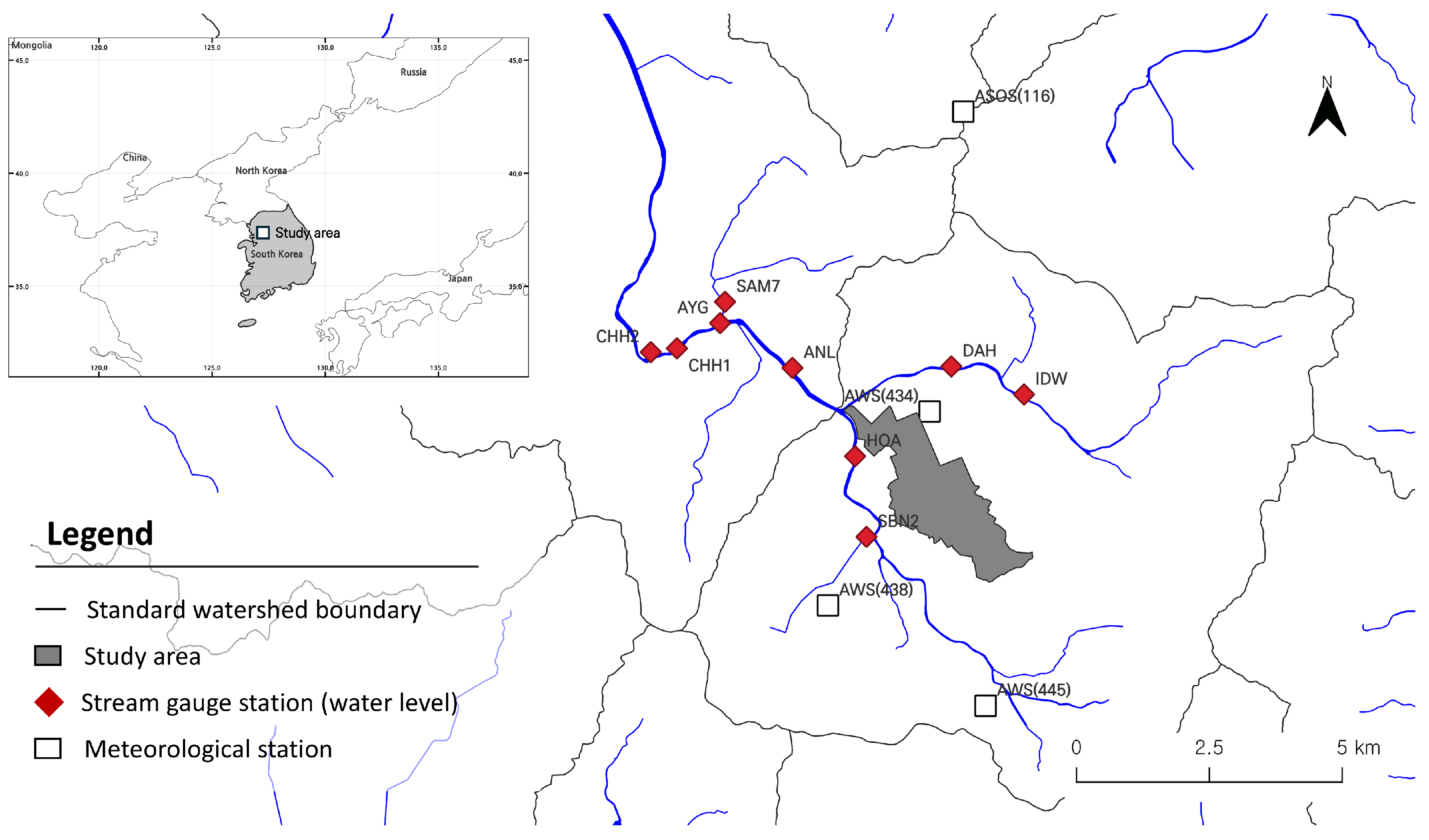
The study area is located in Bisan-dong, Anyang City, South Korea, and encompasses the confluence of the Anyang Stream and the Hagui Stream. This low-lying urban zone has experienced recurrent flooding in recent years (Figure 1). The contributing drainage area to the confluence is approximately 4.11 ${\mathrm{km}}^2$, with an average elevation of 61 $\mathrm{m}$, as derived from a digital elevation model (DEM).

Along the Anyang Stream, six stream gauge stations are operated by Anyang City, and two additional stream gauges are installed along the Hagui Stream. The gauges are located near key bridge crossings (e.g., Anil, Sanbon 2, Anyang, Hoan, Daehan, Chunhun, Samsung 7, and Indeogwon Bridges), forming a dense longitudinal network for monitoring stage dynamics in the urban reach. Water-level observations from these stream gauges are not publicly accessible as open data; however, they can be obtained upon request via the national Open Data Portal (https://www.data.go.kr/en/index.do, accessed on 29 October 2025), subject to approval by the data provider.

Rainfall and meteorological data were obtained from four nearby Korea Meteorological Administration (KMA) stations, including both Automated Synoptic Observing System (ASOS) and Automatic Weather Station (AWS) sites (https://data.kma.go.kr/resources/html/en/aowdp.html, accessed on 29 October 2025). These data are provided by KMA at a 10 min temporal resolution. KMA performs its own internal quality-control procedures before releasing the datasets. Therefore, no additional quality control was applied in this study. In this work, the rainfall and stream-stage observations were used exclusively to train and validate the deep learning-based stream-stage forecasting model. The rainfall time series and stream-stage time series served as input and target series, respectively, for short-lead stage forecasting. In contrast, the inundation surrogate model was trained solely on outputs from hydrodynamic simulations and did not directly use the observational time series. The observation period for the stream-stage forecasting model spanned 2011–2018 for training and 2019–2022 for independent validation.

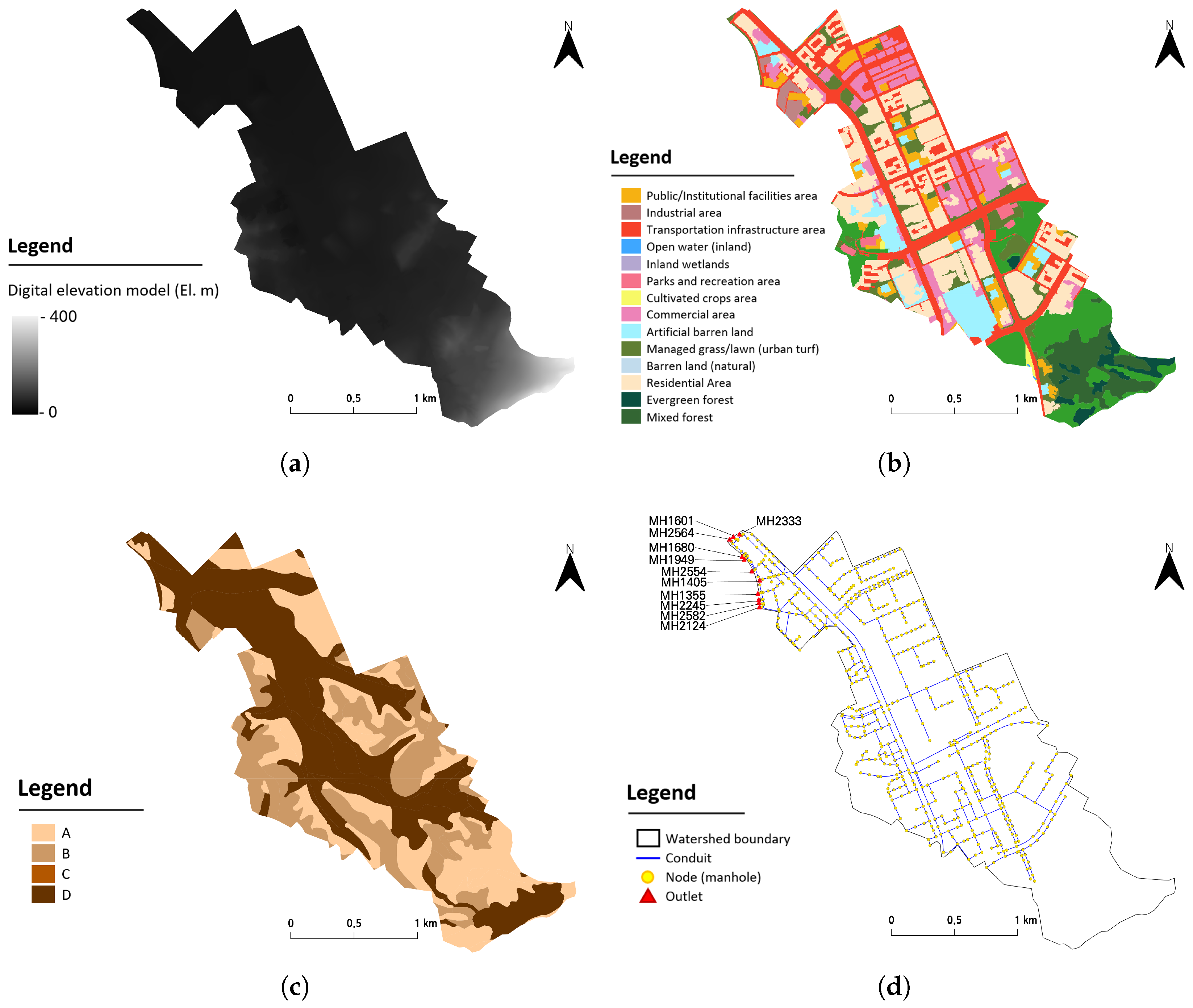
The watershed is highly urbanized (Figure 2). Land-cover analysis indicates that approximately 65% of the basin is covered by residential, commercial, and industrial land uses, while only 32% corresponds to planned park areas and upstream forested hillslopes. As a result, most of the surface is impervious, promoting rapid runoff generation and short hydrological response times during intense rainfall events. Stormwater in the study area is collected by an underground storm sewer network and discharged through 11 outfalls. The nine outlets convey stormwater directly into the Anyang Stream, whereas two outlets discharge into the Hagui Stream, resulting in an asymmetric drainage configuration that tends to concentrate flows toward the Anyang Stream near the confluence.

Evidence of major flood events in the Bisan-dong confluence area was derived primarily from contemporary news reports [20,21,22,23]. National and local media have repeatedly documented severe inundation of apartment complexes, underground parking garages, and adjacent roadways in Bisan-dong during intense summer rainfall events, including the 8–9 August 2022 event along the Anyang Stream. This combination of dense urban development, high imperviousness, complex drainage–channel interactions, and repeatedly reported flood damage makes the area a representative test bed for evaluating the proposed AI-based stream-stage forecasting model and the hydrodynamic-simulation-based inundation surrogate for urban flood forecasting.

2.2. Deep Learning-Based Stream-Stage Forecasting

2.2.1. Input Data and Problem Formulation

The objective of the deep learning model is to predict short-lead stream stage at urban gauge locations from recent histories of rainfall and water level. Time series from three Korea Meteorological Administration (KMA) rainfall stations (Suwon, Gwanaksan, and Uiwang ASOS/AWS), together with stage observations from four stream gauges along the Anyang Stream (Anil, Hoan, Daehan, and Anyang Bridges), are used as predictors. All rainfall and stage records are available at a 10 min temporal resolution. For each prediction time t, an 18-step (3-h) input window is constructed, covering the interval $[t-17,\dots ,t]$. The resulting predictor vector at time t is therefore a sequence of length 18 with 7 features (3 rainfall series + 4 stage series), which can be expressed as

$${\mathbf{X}}_t=\left\{{\mathbf{x}}_{t-17},\dots ,{\mathbf{x}}_t\right\},{\mathbf{x}}_k\in {\mathbb{R}}^d$$

(1)

where ${\mathbf{x}}_k$ is the d-dimensional feature vector at time step k.

The target variable is the stage at a selected gauge for lead times $\Delta \in \{10,20,30,60\}$ min, denoted by $h_{t+\Delta }$. A multi-horizon formulation is adopted, and the network is trained to output all four lead times simultaneously:

$${\widehat{\mathbf{h}}}_t=\left[\begin{array}{c}{\widehat{h}}_{t+10},{\widehat{h}}_{t+20},{\widehat{h}}_{t+30},{\widehat{h}}_{t+60}\end{array}\right]$$

(2)

Separate models can be trained for different target gauges while using the same input configuration.

2.2.2. Network Architecture

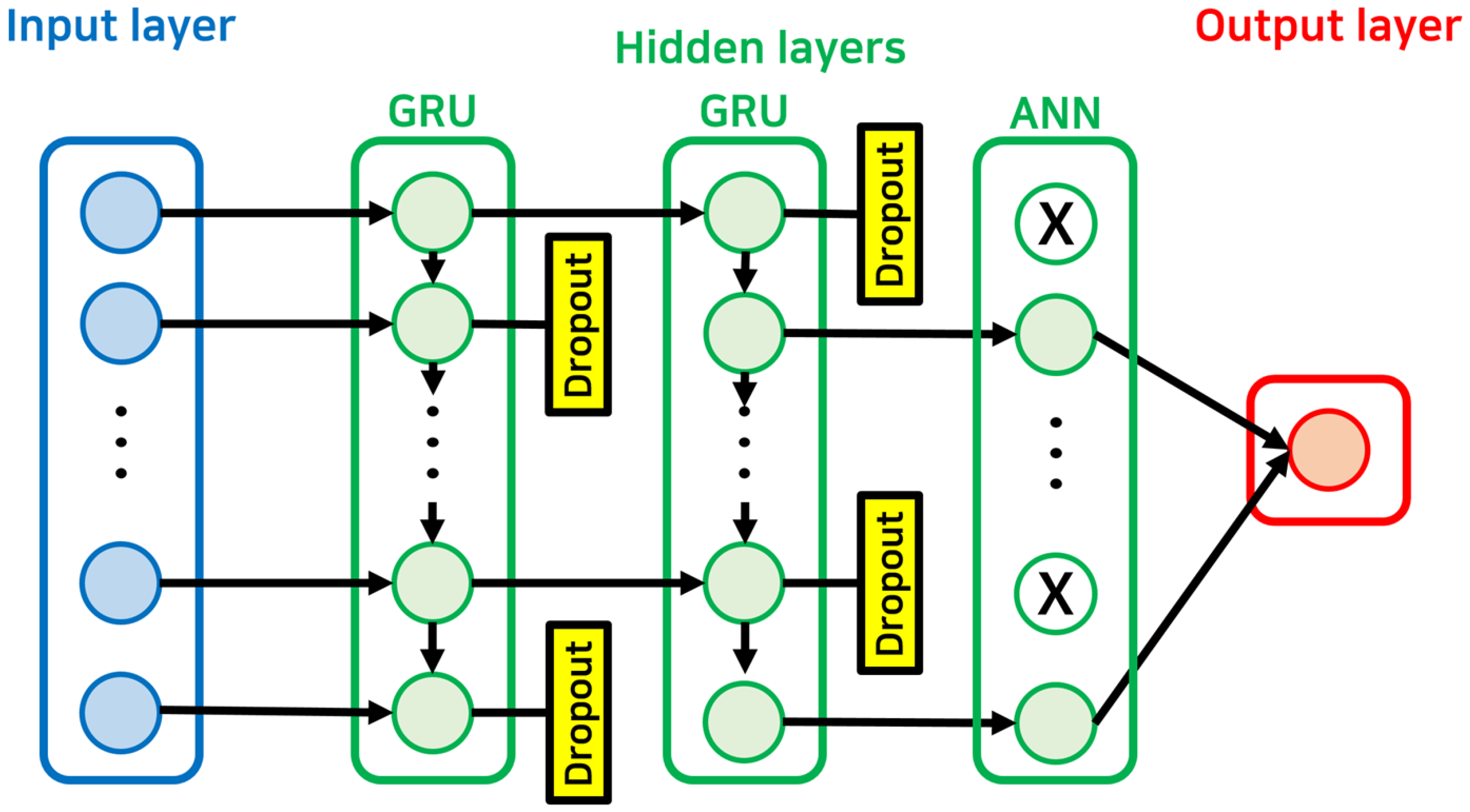
The forecasting model is based on a gated recurrent unit (GRU) network, which was chosen to capture nonlinear temporal dependencies in hydro-meteorological series while maintaining a relatively compact parameterization compared with long short-term memory (LSTM) networks. The final architecture follows a GRU–GRU–ANN structure with three hidden layers (Figure 3).

The first GRU layer receives the input sequence ${\mathbf{X}}_t$ and produces a full sequence of hidden states. A second GRU layer is stacked on top of the first layer and takes this hidden sequence as its input. This second GRU layer returns only the last hidden state, which provides a compact summary vector representing the 3 h history of rainfall and stream stage.

The summary vector is then passed to a fully connected (ANN) layer, which maps the GRU-derived features into a latent representation suitable for regression. Finally, an output layer with four neurons and linear activation produces stream-stage forecasts at 10, 20, 30, and 60 min ahead.

To mitigate overfitting, dropout and $L_2$ weight regularization are applied to the dense part of the network. In this study, a dropout rate of 0.2 is used in the fully connected layer, while the GRU layers are kept intact to preserve temporal dependencies.

2.2.3. Training Procedure

The GRU network is implemented in TensorFlow/Keras and trained using backpropagation through time with the Adam optimizer and a fixed learning rate of 0.001. The mean squared error (MSE) between the observed and predicted stages across all four lead times is used as the loss function.

Data from 2011 to 2018 are used for training, and data from 2019 to 2022 are reserved for independent validation, consistent with the hydrologic analysis periods used elsewhere in this study. Within the training period, 20% of the samples are randomly selected as an internal validation subset for early stopping. The hyperparameter set with the lowest validation loss is retained.

The GRU model hyperparameters were determined by manual, trial-and-error tuning. Key settings, including input sequence length, the number of GRU layers and hidden units, dropout rate, learning rate, and batch size, were iteratively adjusted, and the final configuration was selected based on stable validation behavior and consistent error reduction across forecast horizons. The final hyperparameter set was then fixed and applied consistently to all gauges and lead times. Specifically, the model used an input sequence length of 18 (10 min steps), a dropout rate of 0.2, the Adam optimizer with a learning rate of 0.001, a batch size of 1000, and early stopping with a patience of 100 epochs.

2.2.4. Performance Metrics

The predictive performance of the GRU model at each lead time is evaluated using three complementary metrics widely employed in hydrological modeling: the coefficient of determination (R²), the mean absolute percentage error (MAPE), and the Nash–Sutcliffe efficiency (NSE).

The coefficient of determination R² quantifies the fraction of variance in the observed stage explained by the model, with values closer to 1 indicating better agreement. The mean absolute percentage error is defined as

$$\mathrm{MAPE}={\displaystyle \frac{100}{M}}\sum _{j=1}^M\left|{\displaystyle \frac{h_j-{\widehat{h}}_j}{h_j}}\right|$$

(3)

where $h_j$ and ${\widehat{h}}_j$ denote the observed and predicted stages at time step j, respectively, and M is the number of time steps considered. Lower MAPE values (approaching 0%) indicate smaller relative errors.

The Nash–Sutcliffe efficiency (NSE) compares the predictive performance of the model with that of a baseline that always predicts the mean observed stage:

$$\mathrm{NSE}=1-{\displaystyle \frac{{\sum }_{j=1}^M{(h_j-{\widehat{h}}_j)}^2}{{\sum }_{j=1}^M{(h_j-\overline{h})}^2}}$$

(4)

where $\overline{h}$ is the mean of the observed stage over the evaluation period. Values of NSE close to 1 indicate excellent performance, whereas values near or below 0 indicate performance comparable with or worse than the baseline.

These metrics are computed separately for the training and validation periods and for each forecast lead time (10, 20, 30, and 60 min), providing a detailed characterization of the lead-time degradation and generalization performance of the GRU-based stream-stage forecasting model.

2.3. Deep Learning-Based Urban Inundation Prediction

2.3.1. Scenario Design and Hydrodynamic Simulations

The deep learning inundation model is designed as a surrogate for a physically based two-dimensional (2D) hydrodynamic model. As a first step, a comprehensive set of synthetic flood events was generated by combining design hyetographs with a range of downstream boundary water levels at storm sewer outfalls.

For rainfall forcing, the third-quartile Huff temporal distribution was adopted, as it is widely used in Korea to represent convective storm patterns. Storm durations of 1, 2, and 3 h were considered. For each duration, total event depths from 30 mm to 200 mm were prescribed at 10 mm increments, resulting in 18 distinct rainfall scenarios. For the downstream boundary, 16 water-level cases were defined at key storm sewer outfalls, ranging from free outflow conditions that do not affect sewer capacity to backwater conditions in which the water level rises from below the pipe invert to the ground surface in 0.5 m increments (

Table 1. Scenario-specific downstream boundary water levels assigned to storm sewer outfalls in the XP-SWMM simulations.

Outlet Name	Downstream Boundary Water Level (El. m)
	Case1	Case2	Case3	Case4	Case5	Case6	Case7	Case8	Case9	Case10	Case11	Case12	Case13	Case14	Case15	Case16
MH1355	29.9	29.4	28.9	28.4	27.9	27.4	26.9	26.4	25.9	25.4	24.9	24.4	23.9	23.4	Free	Free
MH1405	29.8	29.3	28.8	28.3	27.8	27.3	26.8	26.3	25.8	25.3	24.8	24.3	23.8	Free	Free	Free
MH1601	29.4	28.9	28.4	27.9	27.4	26.9	26.4	25.9	25.4	24.9	24.4	23.9	23.4	Free	Free	Free
MH1680	29.6	29.1	28.6	28.1	27.6	27.1	26.6	26.1	25.6	25.1	24.6	24.1	23.6	Free	Free	Free
MH1949	29.7	29.2	28.7	28.2	27.7	27.2	26.7	26.2	25.7	25.2	24.7	24.2	23.7	23.2	Free	Free
MH2124	30	29.5	29	28.5	28	27.5	27	26.5	26	25.5	25	24.5	24	23.5	Free	Free
MH2245	29.9	29.4	28.9	28.4	27.9	27.4	26.9	26.4	25.9	25.4	24.9	24.4	23.9	23.4	Free	Free
MH2333	29.5	29	28.5	28	27.5	27	26.5	26	25.5	25	24.5	24	23.5	Free	Free	Free
MH2554	29.7	29.2	28.7	28.2	27.7	27.2	26.7	26.2	25.7	25.2	24.7	24.2	23.7	23.2	22.7	Free
MH2564	29.3	28.8	28.3	27.8	27.3	26.8	26.3	25.8	25.3	24.8	24.3	23.8	23.3	Free	Free	Free
MH2582	29.9	29.4	28.9	28.4	27.9	27.4	26.9	26.4	25.9	25.4	24.9	24.4	23.9	23.4	22.9	Free

). The Cartesian product of the 18 rainfall scenarios and 16 downstream boundary conditions yielded 864 hydrologic–hydraulic scenarios, which were used to construct the training dataset for the inundation surrogate model.

Urban runoff and surface inundation under each scenario were simulated using the commercial 1D–2D model XP-SWMM. The model couples a one-dimensional representation of the storm sewer network with a two-dimensional surface flow module defined over a high-resolution digital elevation model (DEM). In this coupled configuration, surcharge or overflow from manholes is routed over the surface, while ponded water can re-enter the sewer system once pipe capacity becomes available. This configuration allows the simultaneous simulation of flows within the underground conveyance system and over the urban surface, providing spatially distributed fields of flood depth and extent for each scenario.

To ensure that the hydrodynamic model reproduces realistic inundation patterns, the XP-SWMM configuration was qualitatively evaluated against the documented impacts of the 8–9 August 2022 flood event in Bisan-dong. When forced with the observed rainfall for this event, the simulated inundation extent and depth around apartment complexes and underground parking garages were consistent with reported damage locations. This agreement provides confidence that the model captures the dominant flow pathways and ponding mechanisms in the study area.

2.3.2. Preparation of Training Labels

For each of the 864 scenarios, the 2D module of XP-SWMM generated a raster map of maximum inundation depth over the study area. The original simulations were conducted on a grid with a spatial resolution of 1 $\mathrm{m}$ × 1 $\mathrm{m}$, yielding more than 11 million cells (11,703,204 cells) per inundation map and resulting in a data volume that is prohibitively large for direct use in deep learning.

To reduce dimensionality while preserving key spatial patterns, the raw inundation rasters were first aggregated to a resolution of 10 $\mathrm{m}$ × 10 $\mathrm{m}$ by averaging cell depths within each 10 m block. The aggregated rasters covering the target urban basin (approximately 12 ${\mathrm{km}}^2$) were then cropped and resampled to square images of size 256 × 256 cells. This resolution is a power of two and is well suited to convolutional neural network (CNN) architectures.

2.3.3. Deep Learning Model Architecture and Training

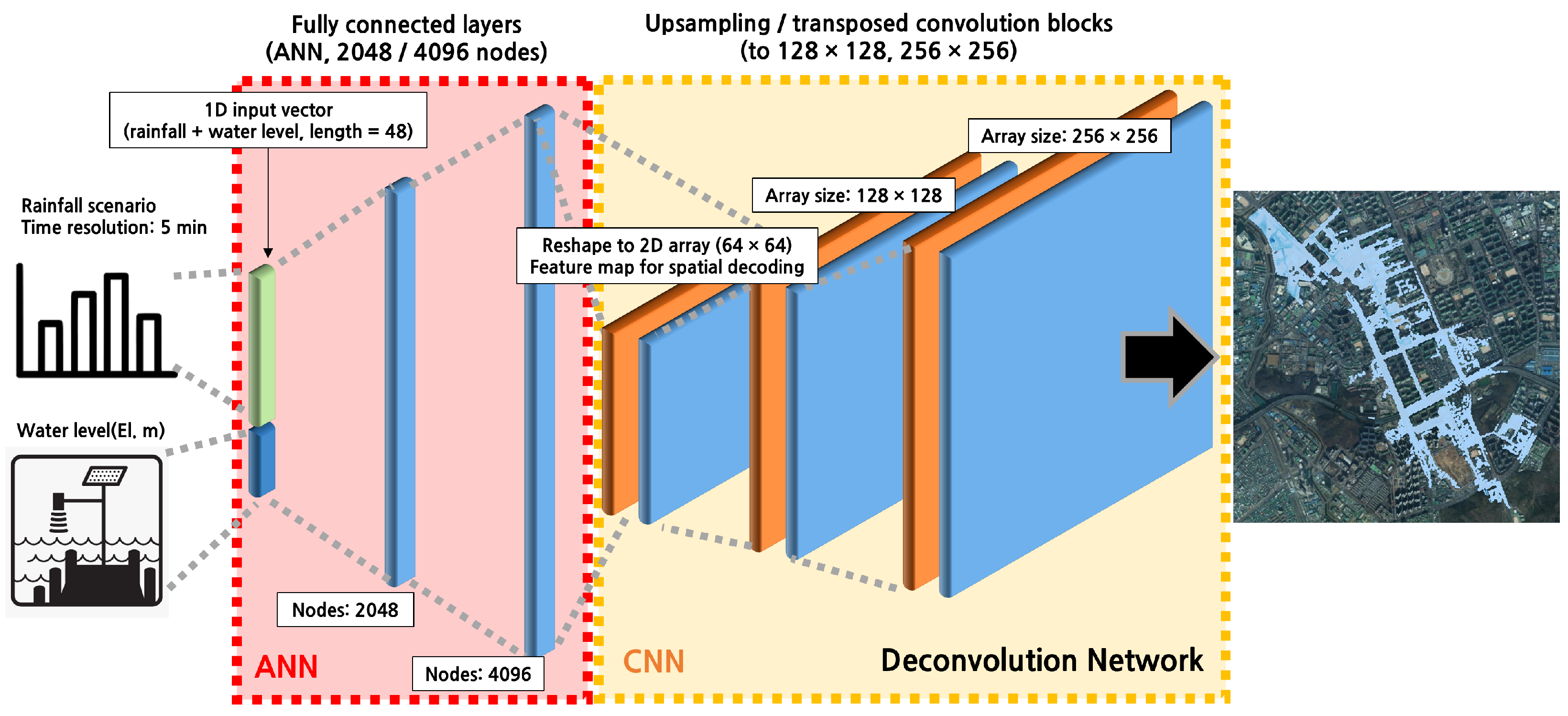
The deep learning inundation surrogate is designed to map compact scenario descriptors to high-resolution flood depth fields on a 256 × 256 computational grid covering the study area. As illustrated in Figure 4, the model follows an encoder–decoder architecture. An ANN encoder transforms one-dimensional hydro-meteorological inputs into a latent feature representation, and a CNN decoder reconstructs the corresponding two-dimensional inundation depth map.

The model is constructed as follows: First, the rainfall and downstream boundary-condition descriptors are assembled as a one-dimensional input vector and normalized. Second, an ANN expands this vector into a higher-dimensional latent representation. Third, the latent vector is reshaped into a low-resolution two-dimensional feature tensor. Finally, a CNN-based decoder progressively upsamples the tensor to produce a 256 × 256 inundation-depth map consistent with the XP-SWMM simulation outputs.

For each XP-SWMM scenario, the input vector is constructed from the rainfall and downstream boundary conditions used in the hydraulic simulations. The vector includes summary descriptors of the design storm (e.g., total depth, duration, temporal pattern) and indicators of the downstream water-level case at storm sewer outfalls. All input features are standardized using the mean and standard deviation computed from the training set. The standardized vector is then passed through a stack of fully connected layers with rectified linear unit (ReLU) activation functions. This ANN encoder projects the low-dimensional scenario description into a higher-dimensional latent vector, which is reshaped into a coarse two-dimensional feature map.

The CNN decoder takes this feature map and progressively upsamples and refines it to the target resolution of 256 × 256 cells. A sequence of convolution and upsampling (transposed convolution) layers captures local spatial patterns and propagates information across neighboring cells. The final convolution layer has a single output channel with a linear activation function and produces a continuous estimate of maximum inundation depth at each grid cell. Negative values, if any, are truncated to zero during post-processing to maintain physical consistency.

The network is implemented in a modern deep learning framework (e.g., TensorFlow/Keras) and trained using the Adam optimizer with a fixed learning rate of 0.001. The 864 XP-SWMM scenarios are randomly split into training (80%) and validation (20%) sets, ensuring coverage of storm durations, rainfall depths, and downstream boundary conditions in both subsets. Training is performed using mini-batches, and early stopping based on validation loss is applied to prevent overfitting. Dropout is applied in the fully connected layers, and L2 regularization is applied to the convolutional filters. The loss function is defined as the mean squared difference between the predicted and XP-SWMM-simulated inundation depths across all grid cells. Scenario-level performance metrics—for inundation area and grid-based depth—are subsequently evaluated using MAPE.

3. Results

3.1. Water-Level Forecasting

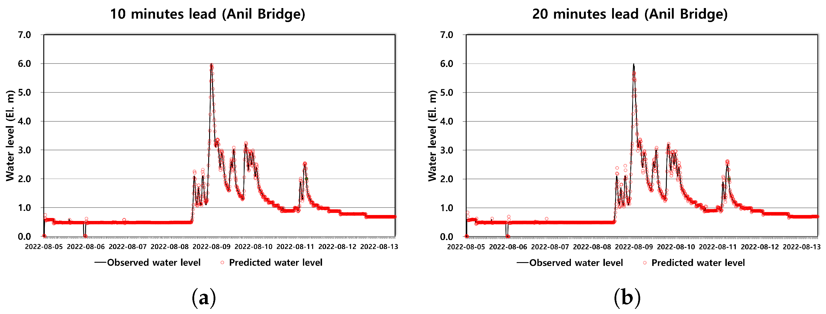
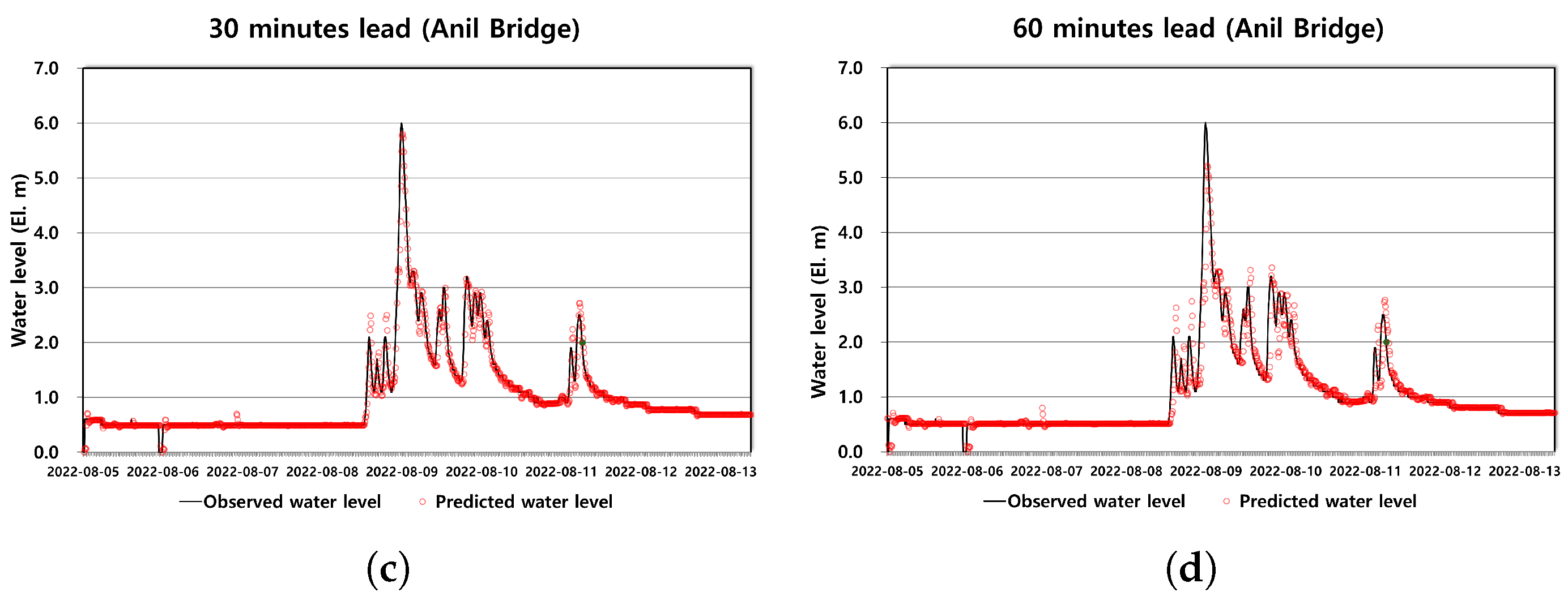
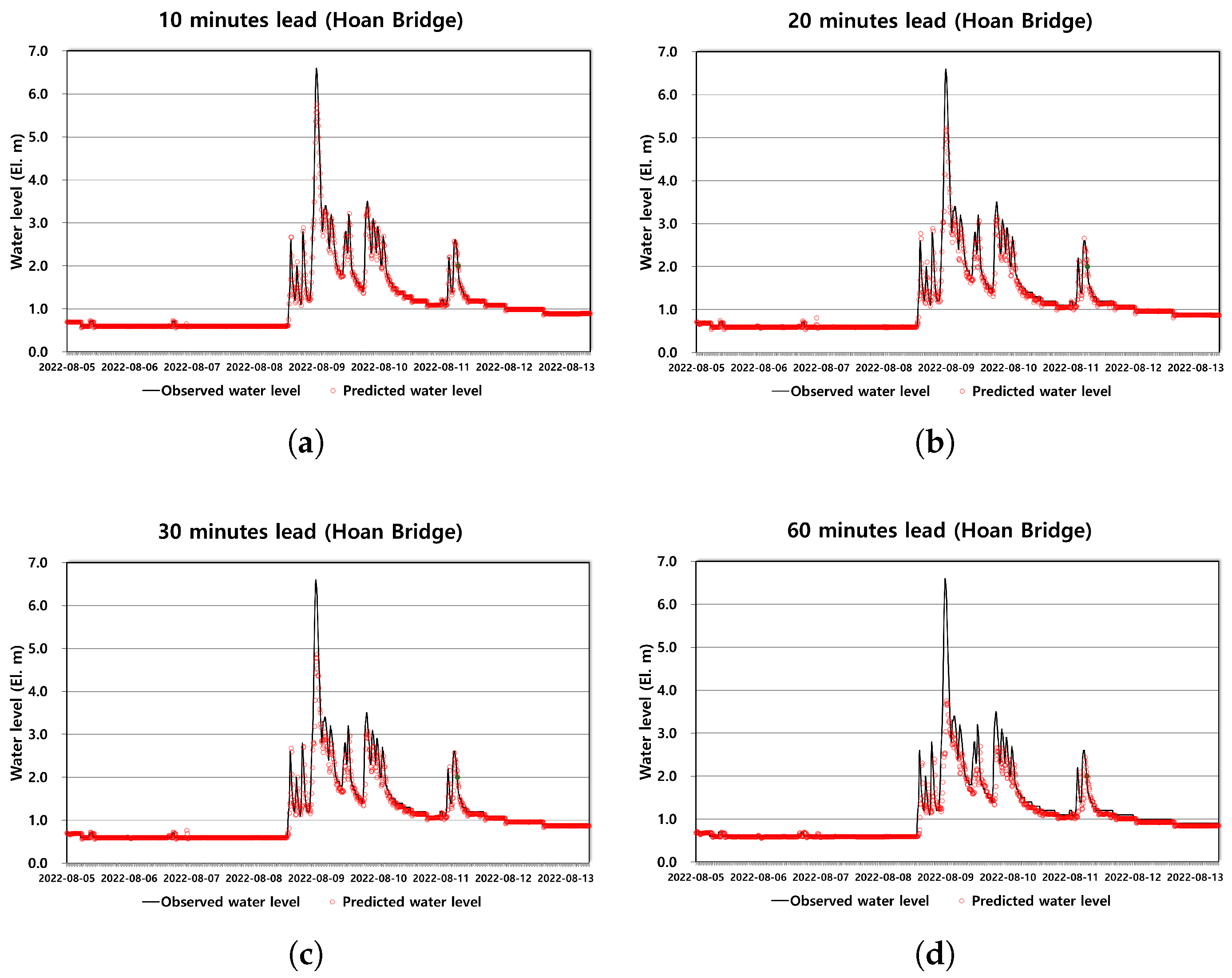
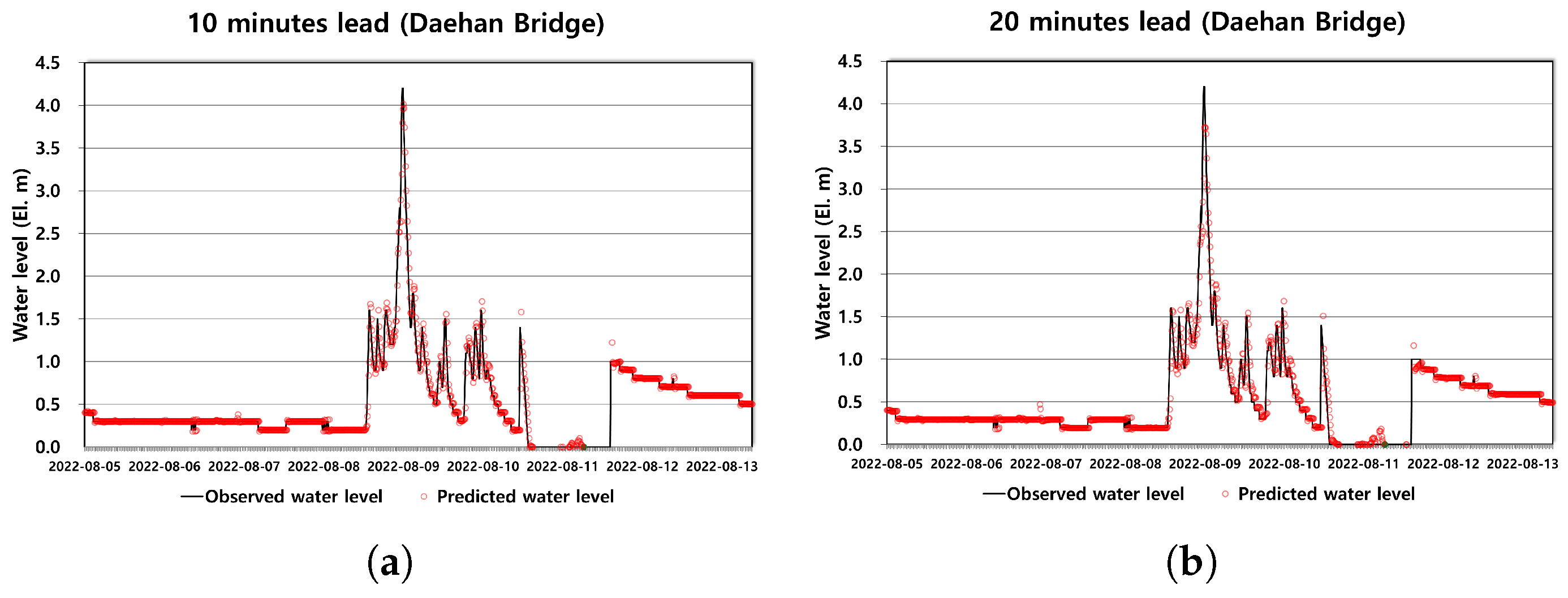
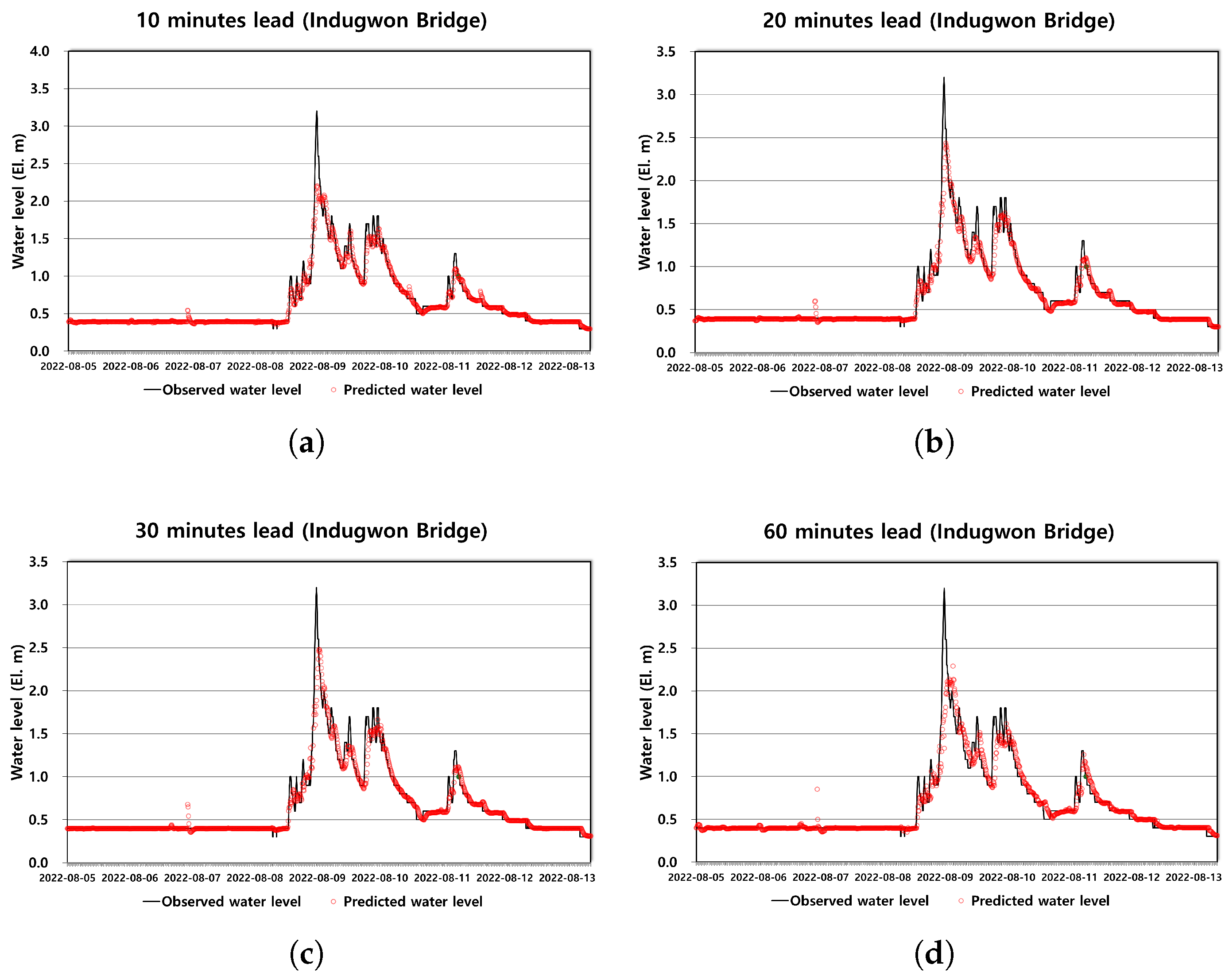
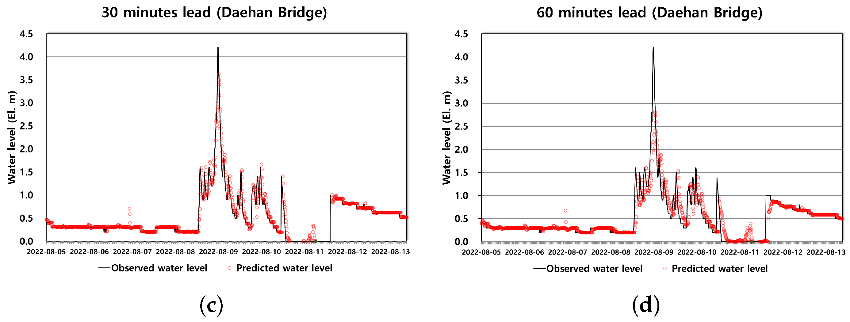
The GRU stream-stage forecasting model was evaluated at four gauging sites along the Anyang–Hagui stream network: Anil Bridge (ANL), Hoan Bridge (HOA), Daehan Bridge (DAH), and Indeogwon Bridge (IDW). For ANL, HOA, and DAH, the period 2011–2018 was used for training and 2019–2022 for independent validation, whereas for IDW—where observations began later—the training and validation periods were 2015–2020 and 2021–2022, respectively. Forecasts were generated at lead times of 10, 20, 30, and 60 min. Model performance was assessed using the mean absolute percentage error (MAPE), the coefficient of determination ($R^2$), and the Nash–Sutcliffe efficiency (NSE). The results are summarized in

Table 2. Performance metrics for training and validation periods (Anil Bridge).

Period	Metric	10 min	20 min	30 min	60 min
Training (2011–2018)	MAPE (%)	2.534	3.467	5.836	11.034
	R2	0.994	0.986	0.962	0.893
	NSE	0.994	0.985	0.9600	0.884
Validation (2019–2022)	MAPE (%)	1.768	2.737	3.427	8.408
	R2	0.994	0.983	0.963	0.875
	NSE	0.994	0.983	0.962	0.872

,

Table 3. Performance metrics for training and validation periods (Hoan Bridge).

Period	Metric	10 min	20 min	30 min	60 min
Training (2011–2018)	MAPE (%)	1.406	5.918	5.214	8.566
	R2	0.987	0.956	0.915	0.775
	NSE	0.987	0.952	0.914	0.773
Validation (2019–2022)	MAPE (%)	1.508	3.172	4.093	7.633
	R2	0.988	0.964	0.928	0.802
	NSE	0.988	0.961	0.924	0.795

,

Table 4. Performance metrics for training and validation periods (Daehan Bridge).

Period	Metric	10 min	20 min	30 min	60 min
Training (2011–2018)	MAPE (%)	1.624	2.005	5.623	4.726
	R2	0.988	0.965	0.926	0.842
	NSE	0.987	0.965	0.908	0.838
Validation (2019–2022)	MAPE (%)	2.527	3.915	6.170	9.033
	R2	0.992	0.976	0.957	0.885
	NSE	0.992	0.976	0.957	0.884

and

Table 5. Performance metrics for training and validation periods (Indugwon Bridge).

Period	Metric	10 min	20 min	30 min	60 min
Training (2011–2018)	MAPE (%)	6.094	7.199	7.390	7.949
	R2	0.796	0.763	0.753	0.733
	NSE	0.795	0.762	0.752	0.731
Validation (2019–2022)	MAPE (%)	4.436	5.069	5.599	6.568
	R2	0.966	0.954	0.944	0.914
	NSE	0.965	0.947	0.939	0.913

and illustrated by the hydrographs in Figure A1, Figure A2, Figure A3 and Figure A4.

At Anil Bridge, the GRU model exhibited very high performance for lead times up to 30 min. During both the training and validation periods, R² and NSE exceeded 0.96 for 10–30 min forecasts, and MAPE remained below 5% in both periods. For short lead times, the model reproduced the timing and magnitude of water-level fluctuations with high fidelity, including the rapid rise and recession during extreme events. At a 60 min lead time, however, R² and NSE decreased to approximately 0.88–0.89, and MAPE increased to roughly 8–11%, indicating a clear degradation in predictive performance. The corresponding hydrographs show that 60 min forecasts tend to respond later than the observations and that peak stages are sometimes overestimated relative to the gauge records.

The results at Hoan Bridge were similar regarding the overall performance but exhibited several distinct features. For 10 and 20 min forecasts, R² and NSE again exceeded 0.95 in both periods, while 30 min forecasts maintained values above 0.90. MAPE at HOA was generally low (approximately 1.4–3.9% for 10–30 min), although the increase from 10 to 20 min was more pronounced than at ANL, reflecting a greater sensitivity to lead time. At 60 min, R² and NSE dropped below 0.80, and MAPE increased to around 7–8%. Unlike ANL, the HOA forecasts showed relatively little systematic overestimation; instead, the main deficiencies at the 60 min horizon were delayed response and underestimation of observed peak levels during intense events.

At Daehan Bridge, the GRU model also showed excellent performance at short lead times. During the training period, R² and NSE exceeded 0.96 at 10–20 min and remained above 0.90 at 30 min; in the validation period, all three short-lead horizons (10, 20, and 30 min) achieved R² and NSE values greater than 0.95. MAPE values mainly ranged between 1.6% and 6.2%, comparable with or slightly higher than those at ANL and HOA. As at the other gauges, 60 min forecasts displayed reduced performance, with R² and NSE below 0.90. An interesting feature at DAH is that, during the training period, the 60 min MAPE (4.7%) was slightly lower than the 30 min MAPE (5.6%), even though the correlation-based metrics decreased with lead time. This pattern suggests that error magnitudes remained moderate while timing errors increased. Visual inspection of the hydrographs confirms that 10–30 min forecasts track the observed patterns very closely, whereas 60 min forecasts show delayed peaks and a tendency to underestimate maximum stages.

The results at Indeogwon Bridge differed from those at the other sites because of the relatively short training record. During 2015–2020, R² and NSE remained below 0.80 for all lead times, and MAPE was relatively high (approximately 6–8%), indicating limited learning from the sparse data. In contrast, the validation period (2021–2022) showed markedly improved performance: R² and NSE exceeded 0.94 at all lead times, and MAPE decreased to approximately 4–7%. The forecasts at IDW generally followed the observed stages well, with little systematic overestimation; instead, they tended to slightly underestimate water levels, particularly at peak times and at the 60 min horizon. This pattern suggests that once several significant events became available in the record, the GRU model effectively captured the local hydrological response despite the shorter observation history.

Taken together, the results from the four gauges demonstrate that the GRU architecture is well suited for short-lead (10–30 min) stream-stage nowcasting in this small, rapidly responding urban basin. Across all sites, R² and NSE values above approximately 0.95 and MAPE values typically below 5% at these lead times indicate that the model reliably reproduces both baseflow stages and sharp rises associated with convective storms. Forecast performance decreases systematically at the 60 min lead time, reflecting the intrinsic difficulty of longer-horizon prediction in such flashy catchments. Nevertheless, even the 60 min forecasts exhibit moderate performance and provide useful qualitative guidance on forthcoming high-water conditions. Accordingly, subsequent sections emphasize the 10–30 min forecasts when coupling the GRU outputs with the inundation surrogate model for urban flood nowcasting.

3.2. Inundation Forecasting

The performance of the ANN–CNN surrogate model for urban inundation prediction was evaluated by comparing its outputs with the XP-SWMM 1D–2D simulations used as training labels. As described in Section 2.3, a total of 864 scenarios were generated by combining design storms of different durations and depths with 16 downstream boundary water-level conditions at the storm sewer outfalls. For each scenario, the surrogate generated a 256 × 256 map of maximum inundation depth over the study area. Model performance was assessed using the mean absolute percentage error (MAPE) for total inundation area and grid-based water depth (

Table 6. Mean absolute percentage error (MAPE) for inundation area and grid-based inundation depth.

Category	Inundation Area (MAPE)	Grid-Based Inundation Depth (MAPE)
Overall mean MAPE (%)	8.89	19.49

).

Overall, the ANN–CNN model reproduced the XP-SWMM inundation patterns with good agreement in flood extent and moderate errors in local water depth. The MAPE for inundation area was 8.89%, indicating that the surrogate captured the areal extent of flooding with less than 10% relative error on average across all scenarios. In contrast, the MAPE for grid-based depth was 19.49%, reflecting larger discrepancies at the cell scale.

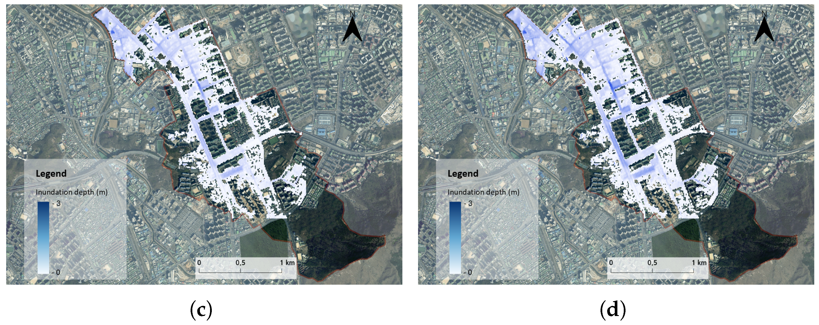
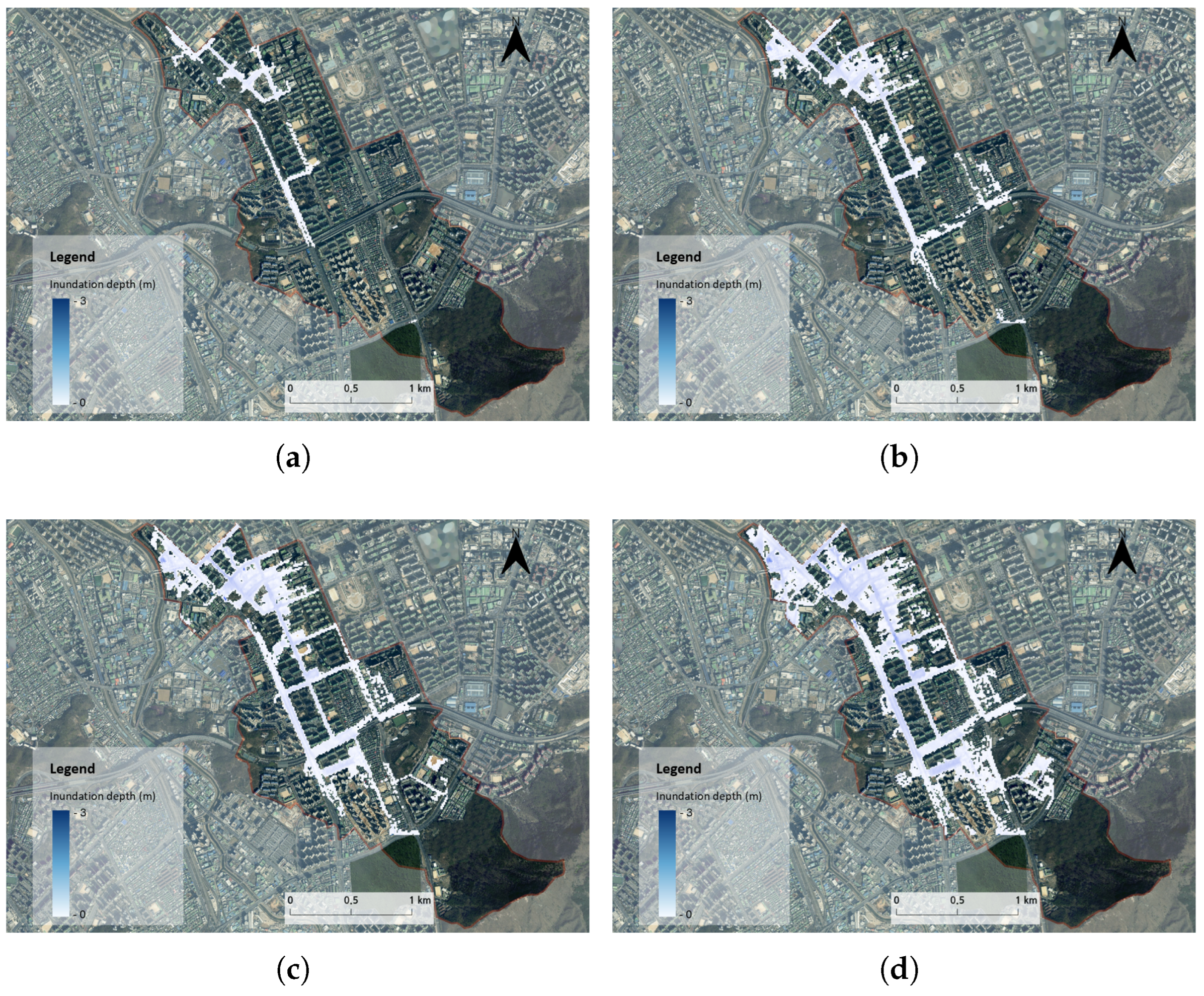
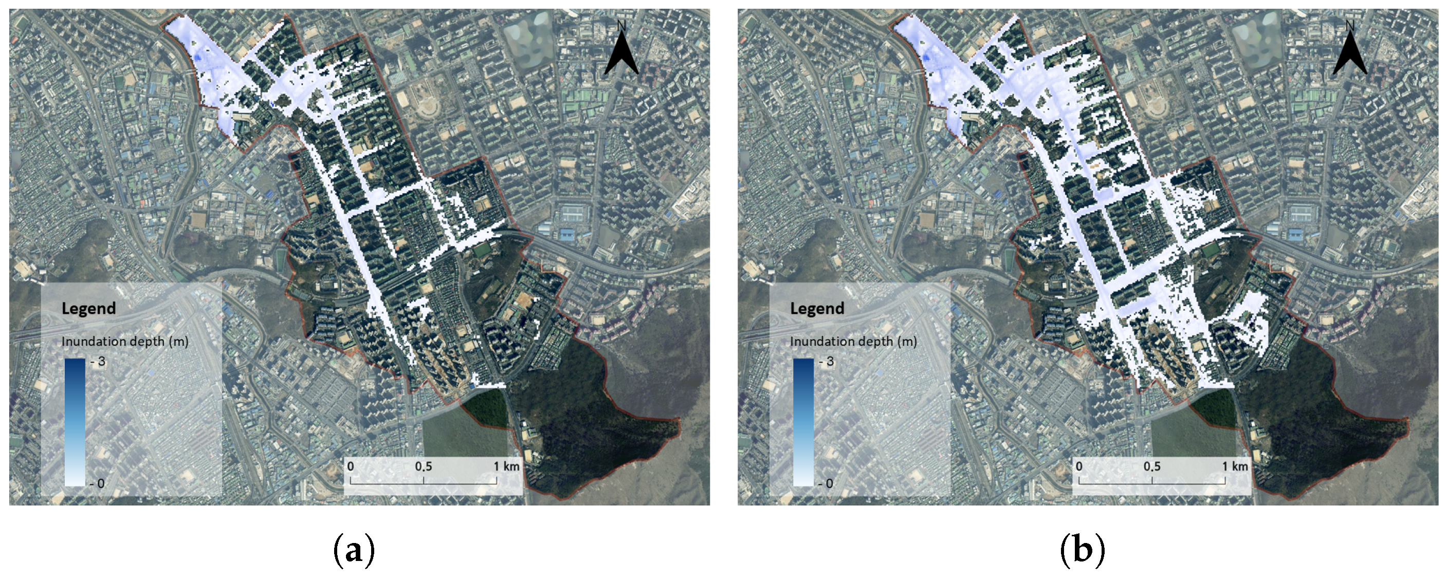
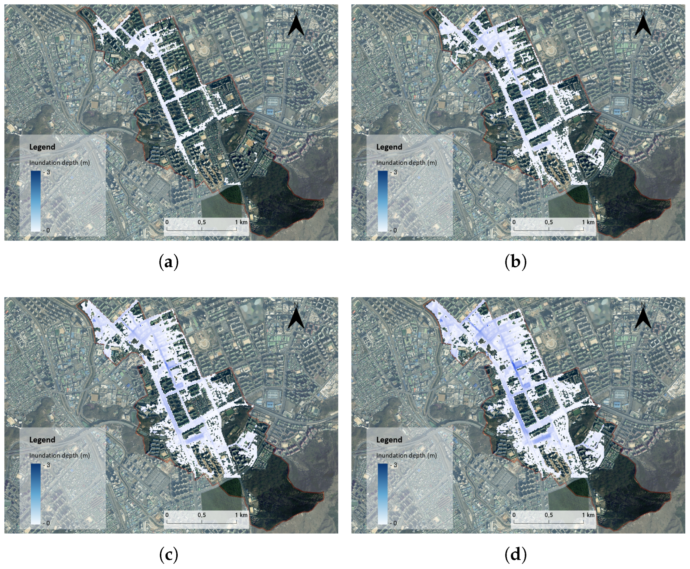
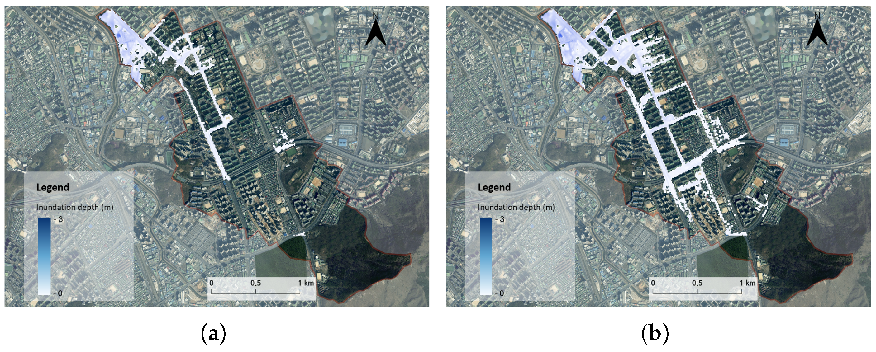
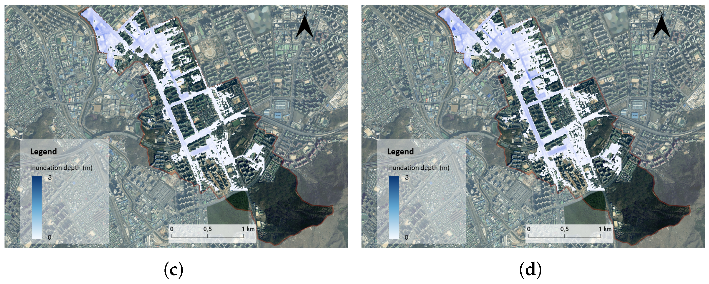
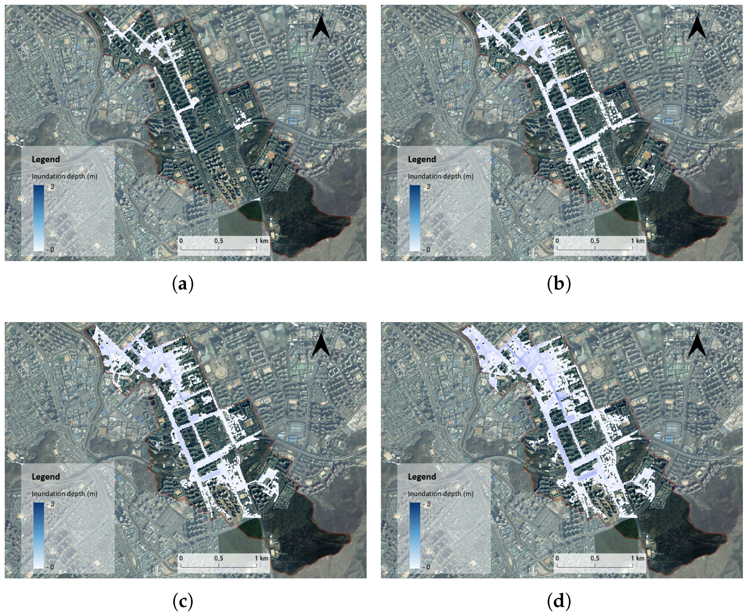
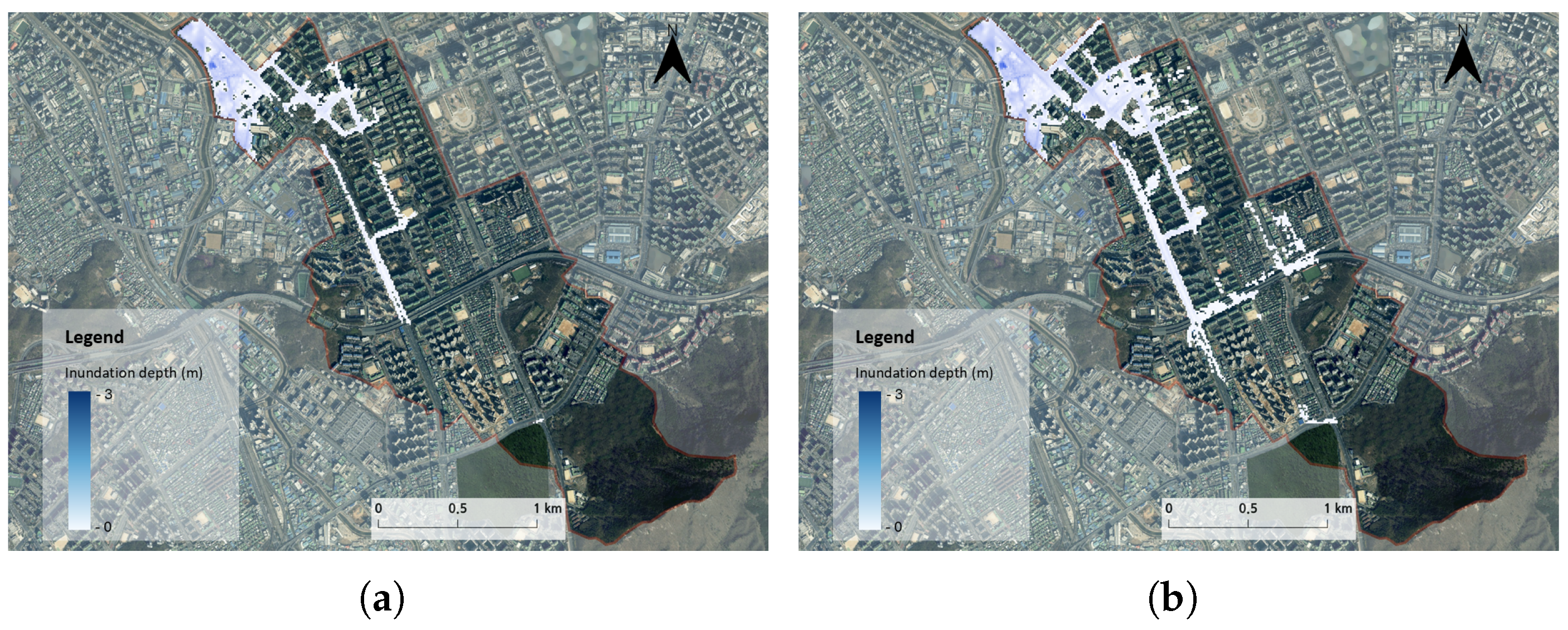
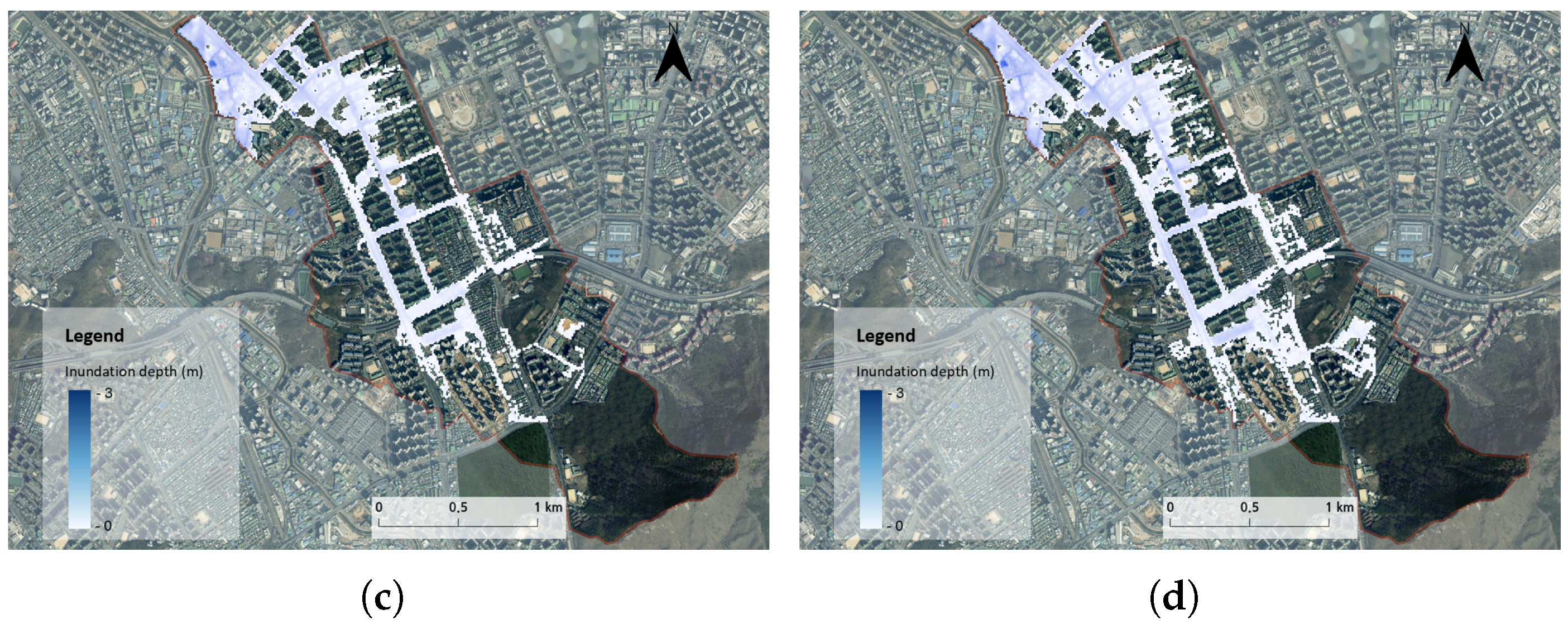
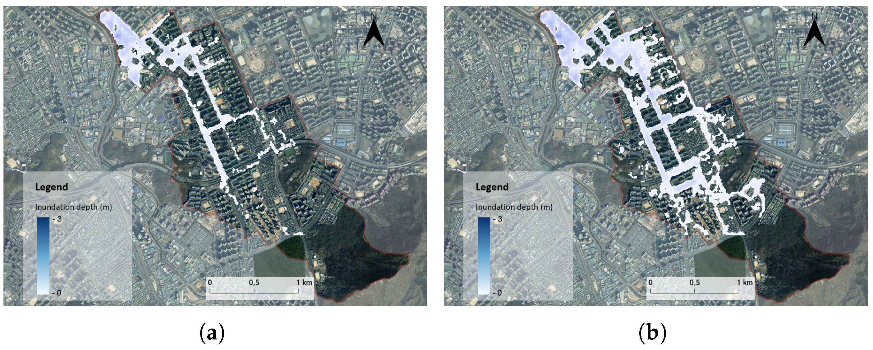
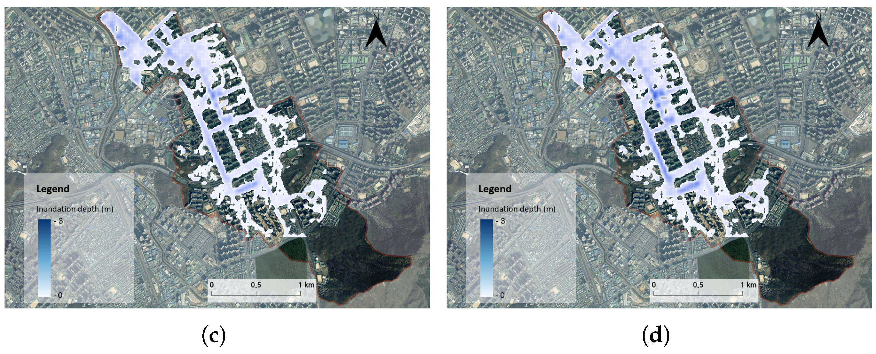
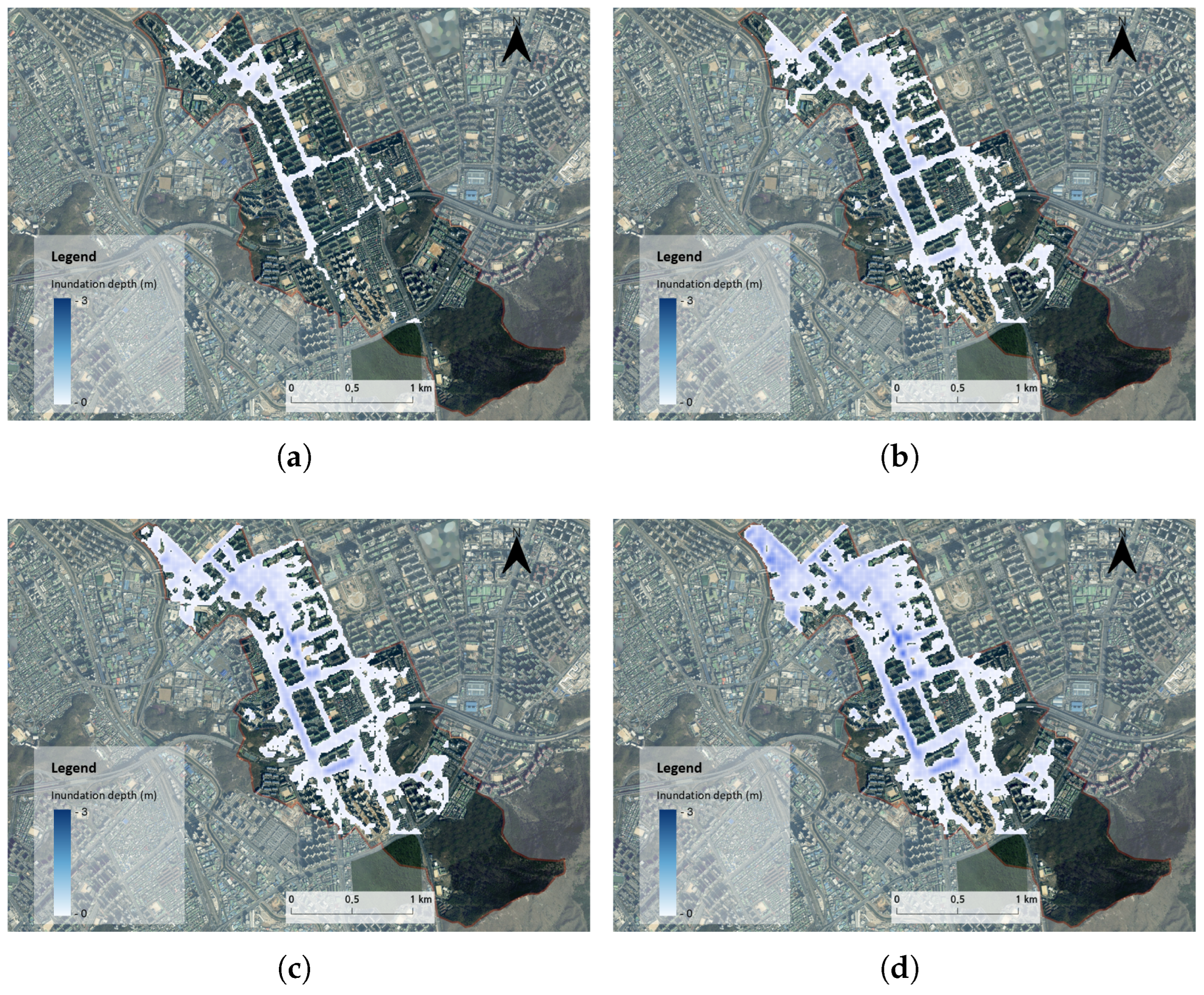
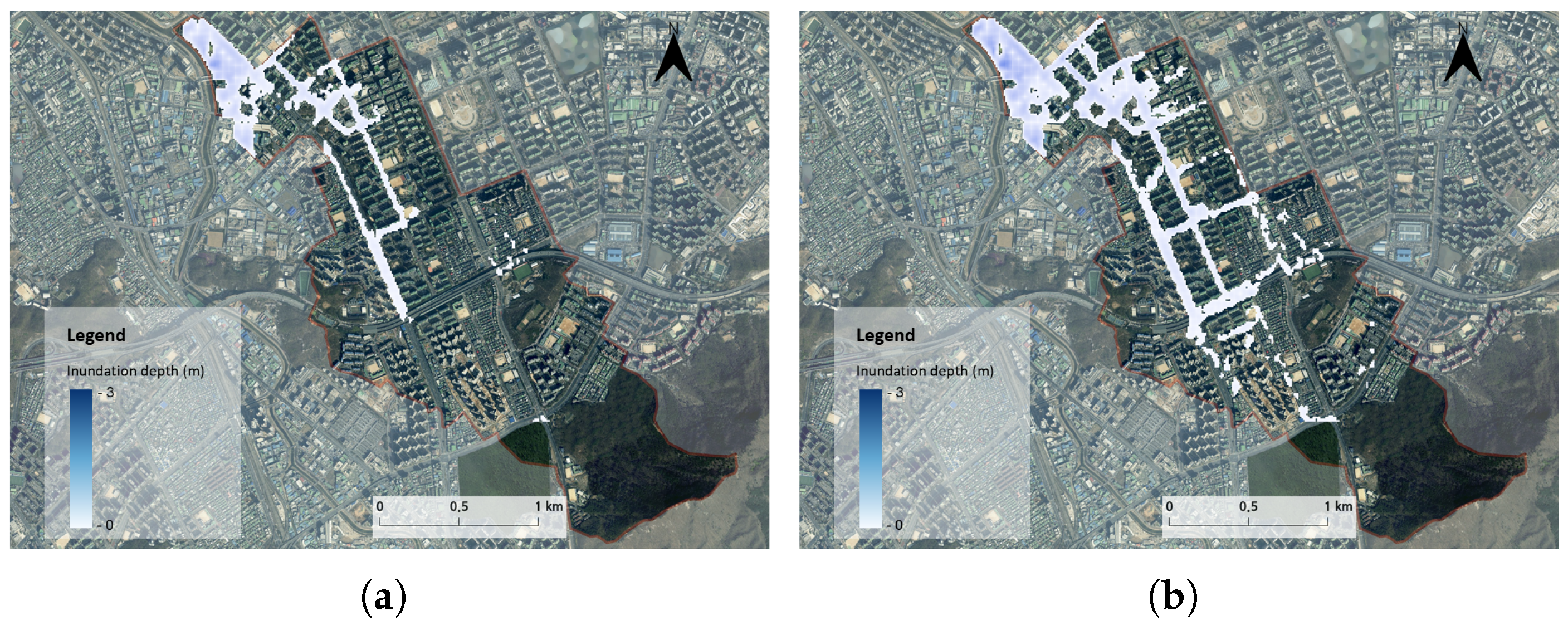
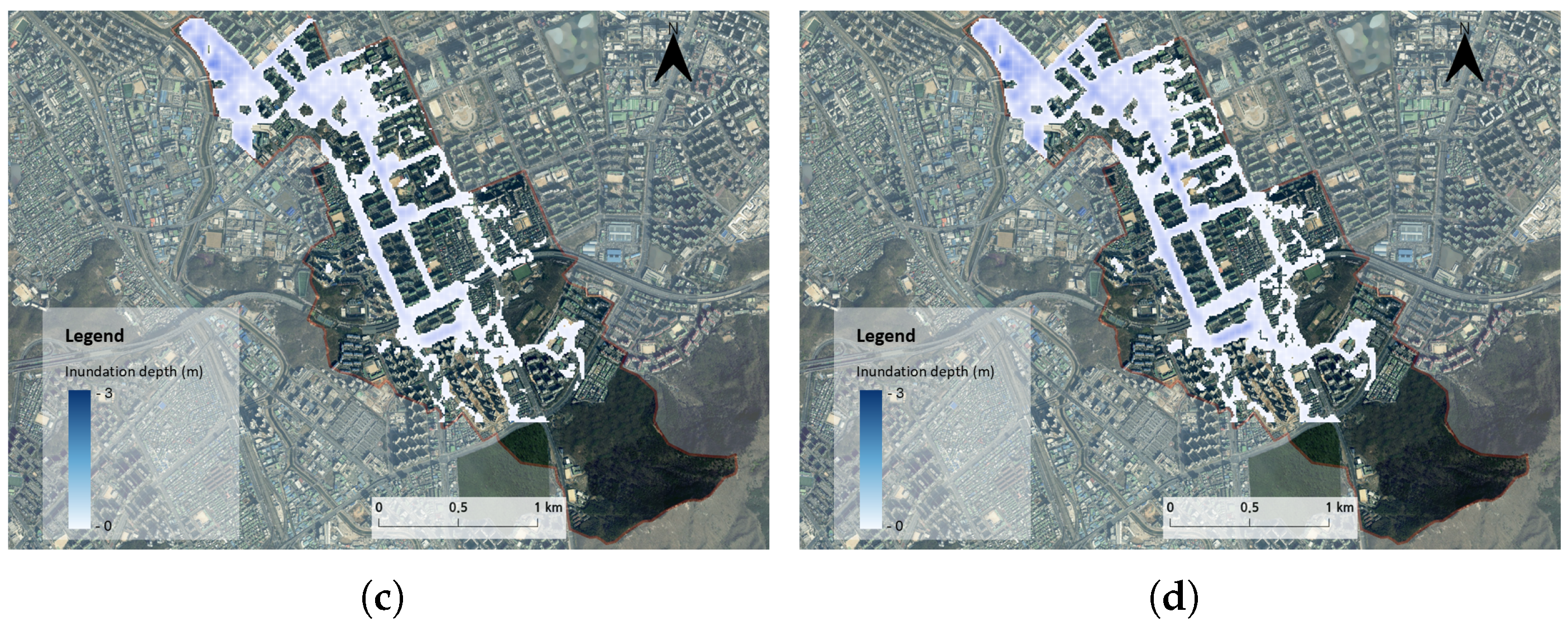
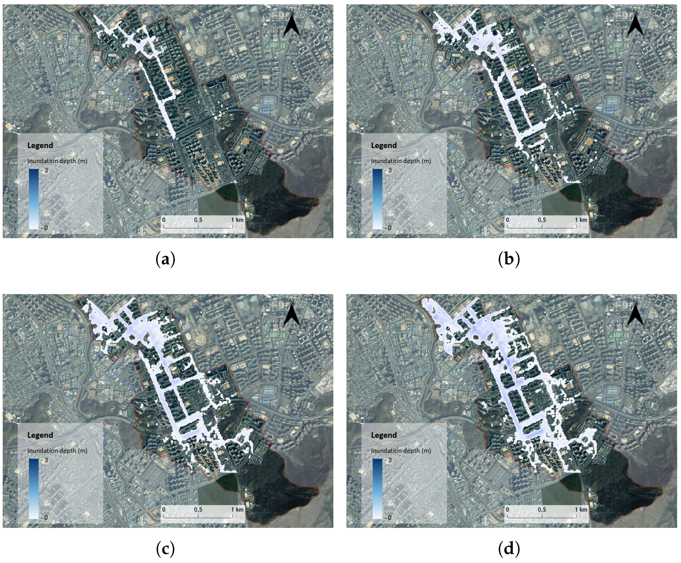
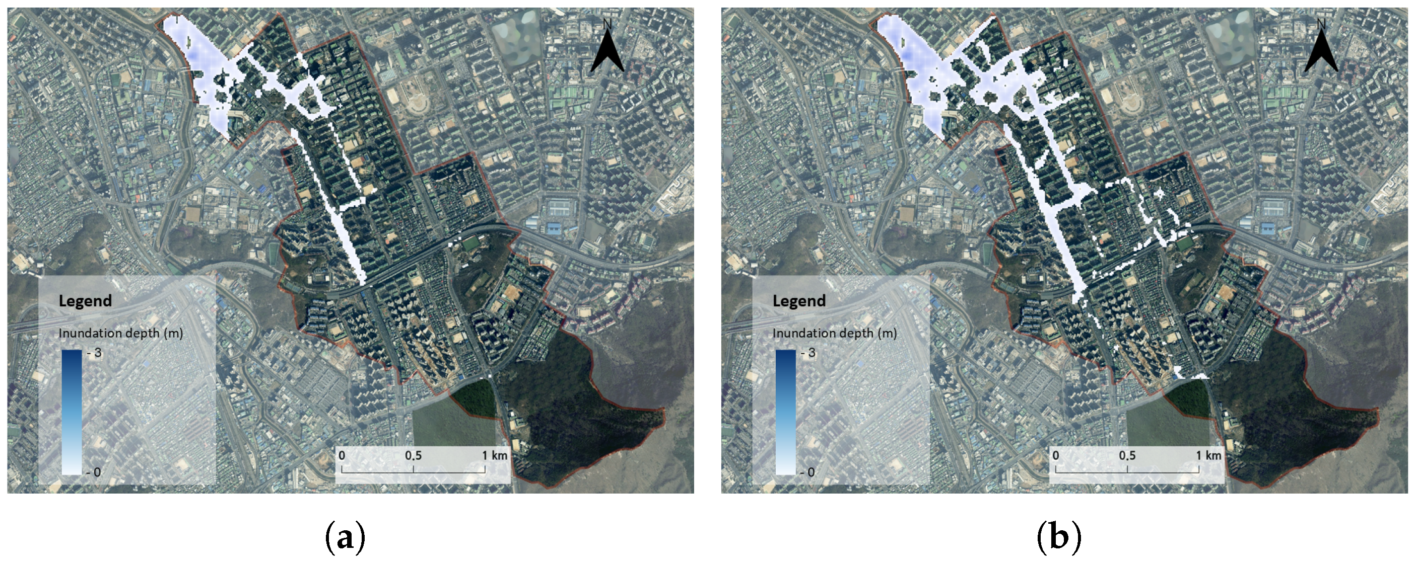
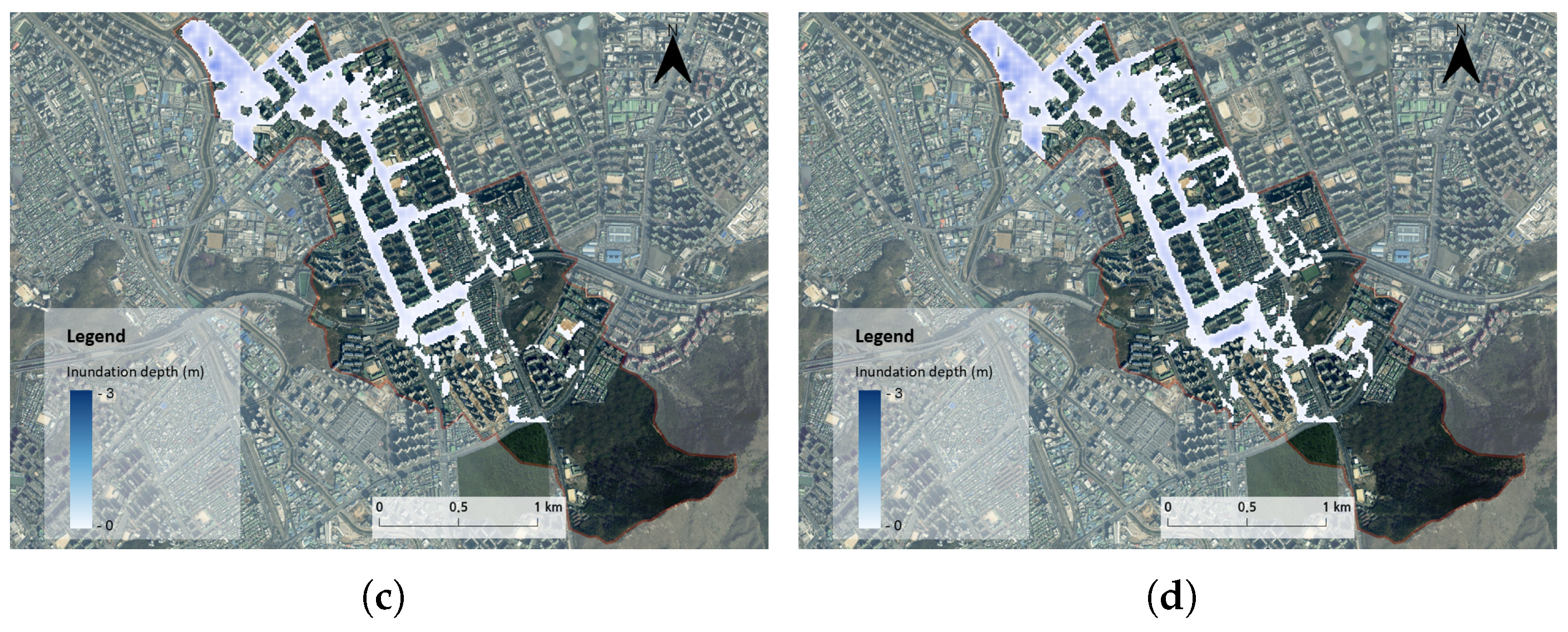
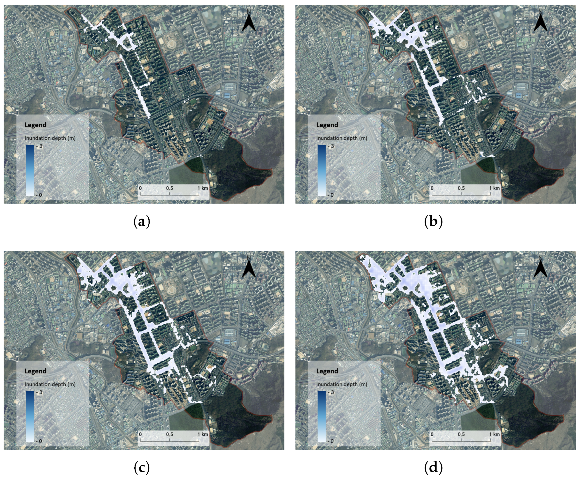
Qualitative comparisons between XP-SWMM simulations (Appendix A.2, Figure A5, Figure A6, Figure A7, Figure A8, Figure A9 and Figure A10) and AI-predicted inundation maps (Appendix A.3, Figure A11, Figure A12, Figure A13, Figure A14, Figure A15 and Figure A16) further support these findings. For low and high downstream boundary water levels (Table 1) and storm durations of 1–3 h with total rainfall ranging from 50 to 200 mm, the surrogate correctly identified the main flood-prone streets, intersections, and low-lying blocks. As rainfall depth and downstream water level increased, both models showed a consistent expansion of inundated areas toward upstream sections and adjacent areas. Differences were more evident in narrow flow paths and small depressions, where the ANN–CNN output tended to smooth sharp gradients and slightly underestimate peak water depths, particularly under the most intense storm and backwater conditions.

Despite these local discrepancies, the surrogate model strikes a useful balance between accuracy and computational efficiency. Once trained, the ANN–CNN model generates high-resolution inundation maps in near real time for new combinations of rainfall and boundary conditions, whereas running the full XP-SWMM model for the same scenario ensemble would be computationally expensive. For many practical applications—such as identifying flood hotspots, screening structural and non-structural measures, or supporting nowcasting-based risk communication—the achieved accuracy in inundation area and depth is sufficient to inform decision-making. However, for detailed hydraulic design at specific locations (e.g., sizing critical drainage structures), use of the complete hydrodynamic model remains advisable.

In summary, the results in Table 6 and Appendix A.2 and Appendix A.3 demonstrate that the proposed ANN–CNN surrogate is capable of emulating a complex dual-drainage model over a wide range of rainfall and downstream boundary scenarios. When coupled with the GRU-based stream-stage forecasts, this capability forms the basis for rapid, scenario-based urban flood nowcasting in the Bisan-dong study area.

4. Discussion

The results of this study demonstrate that a GRU-based short-term stream-stage forecasting model and an ANN–CNN inundation surrogate trained on XP-SWMM simulations can achieve practical performance for urban flood prediction. For stream-stage forecasting, the GRU model achieved high coefficients of determination and Nash–Sutcliffe efficiencies, along with low error rates, at very short lead times of 10–30 min, suggesting that the GRU effectively learns nonlinear temporal dependencies in rainfall–stage time series. In contrast, performance degraded at 60 min lead times, and the predicted peak stages tended to be delayed or insufficiently reproduced. This behavior can be attributed to the combined effects of flashy urban catchment characteristics (e.g., a time of concentration of approximately one hour) and increasing uncertainty in future rainfall.

In highly urbanized basins such as the study site, runoff generation and stage rise occur rapidly during short-duration storms with abrupt changes in rainfall intensity, and water levels frequently surge and recede within tens of minutes. Accordingly, at longer lead times (e.g., 60 min), post-forecast rainfall variability and drainage–channel interactions exert a more decisive influence, and uncertainty in recurrent neural network-based models driven solely by rainfall and stage time-series increases. Peak values, in particular, occur infrequently and are therefore underrepresented in the training data; moreover, training procedures that minimize average errors often result in smoothed peaks and lagged peak timing. Differences in predictive performance among gauging stations may also reflect variations in observation quality (e.g., measurement noise) and drainage conditions, including backwater effects. These factors should be examined more rigorously in future work using longer observation records, improved data quality, and the inclusion of additional explanatory variables.

For inundation prediction, the surrogate model yielded a relatively low MAPE for inundation area (8.89%) but a higher MAPE for grid-based inundation depth (19.49%), reflecting the inherent difference in difficulty between predicting flood extent and predicting localized depth. Inundation area has a quasi-classification character when defined by a threshold (e.g., depth > 0) and is therefore more stable, whereas inundation depth is a continuous variable for which small spatial displacements or subtle boundary shifts can translate into substantial cell-wise relative errors. Errors can be amplified near flood boundaries, where depths are close to zero, and in locations with strong micro-topographic controls (e.g., roads, intersections, and local depressions), where steep depth gradients exist and where the surrogate may represent boundaries and peak depths more smoothly.

In addition, because the inundation surrogate uses scenario descriptors that summarize rainfall and downstream boundary conditions as inputs, it has limited ability to represent differences in runoff and inundation responses arising from finer-scale variations in rainfall temporal patterns or spatial distributions, even for identical total rainfall. Notably, the “ground truth” for the surrogate is not observed inundation but rather the XP-SWMM 1D–2D simulation outputs. Therefore, surrogate accuracy ultimately depends on the assumptions of the physics-based model, the quality of sewer-network and topographic datasets, parameter settings, and boundary-condition specifications. While the ability of the surrogate to closely emulate XP-SWMM results is a significant operational advantage, the possibility that uncertainties in the physics-based model may be inherited by the surrogate should also be acknowledged.

Despite these limitations, the proposed approach offers clear advantages aligned with practical needs in urban flood prediction. Detailed 1D–2D hydrodynamic models can reproduce scenario-specific inundation processes with high fidelity, but their computational cost often restricts real-time operation. In contrast, once trained, the ANN–CNN surrogate can generate high-resolution inundation depth maps very rapidly for the same input conditions, enabling timely situational awareness and decision support. The GRU-based stage nowcasting also showed strong performance at very short lead times, indicating its potential use for early warning and rapid response within the 10–30 min window (e.g., road closures, proactive drainage operation at vulnerable locations, and deployment of emergency resources). Nonetheless, the surrogate is not intended to fully replace the physics-based model; rather, its primary value lies in complementing hydrodynamic simulations by overcoming computational constraints and enabling rapid flood-map production during operations. For applications requiring high-precision hydraulic analysis, such as detailed infrastructure design or site-specific depth estimation, physics-based modeling remains essential, whereas the surrogate is better suited for rapid hotspot identification, scenario screening, and operational decision support.

Several limitations of this study warrant further investigation. First, the analysis is based on a single case study focused on the Bisan-dong confluence area; therefore, additional validation is required to assess generalization to other urban basins. Second, the stage forecasting model relies primarily on rainfall and stage time series and does not incorporate additional predictors that may improve longer-lead performance, such as radar rainfall fields, numerical weather prediction outputs, upstream discharge, or soil moisture states; this limitation may partly explain reduced peak fidelity at lead times of 60 min or longer. Third, because the inundation surrogate was trained on XP-SWMM simulations, direct validation against observation-based flood marks or inundation maps is limited, and uncertainties in XP-SWMM inputs (e.g., sewer-network data, terrain representation, and roughness parameters) can affect the results. Future work should therefore focus on improving longer-lead forecasting by integrating radar- and forecast-based rainfall and downstream-stage predictions, enhancing peak reproduction through loss-function design (e.g., peak-weighted or quantile-based losses) and event-based training strategies, improving depth accuracy using multi-scale architectures such as U-Net and boundary-aware loss formulations, and strengthening credibility through hybrid validation that combines simulation outputs with observation-based flood evidence (e.g., flood-mark surveys and inundation maps). With these advancements, the coupled framework of GRU-based stage nowcasting and ANN–CNN inundation surrogates proposed in this study is expected to contribute to real-time flood prediction in fast-responding urban basins and to support the enhancement of urban flood emergency-response systems.

5. Conclusions

This study developed and evaluated a model-informed deep learning framework that couples GRU-based short-lead stream-stage nowcasting with an ANN–CNN inundation surrogate trained on XP-SWMM simulations for a highly urbanized basin. The results demonstrate that the GRU model provides reliable skill for very short lead times (10–30 min), whereas performance degradation at longer lead times highlights the need for additional predictors to improve robustness under rapidly evolving storms. The inundation surrogate successfully reproduced scenario-based inundation extent and depth patterns with practical accuracy, enabling rapid generation of high-resolution inundation maps. Overall, the proposed framework offers a computationally efficient complement to physics-based models and supports time-critical urban flood warning and decision support. Limitations include the single-site case study and the reliance on simulation-based inundation labels; future work should expand evaluation to additional basins, incorporate radar/forecast rainfall and boundary-condition predictions, and strengthen validation using observation-based flood evidence.

References

1. Georgi, B.; Isoard, S.; Asquith, M.; Garzillo, C.; Swart, R.; Timmerman, J. Urban Adaptation to Climate Change in Europe 2016: Transforming Cities in a Changing Climate; Technical Report; ETC CCA: Venice, Italy, 2016. [Google Scholar]
2. Lin, T.; Liu, X.; Song, J.; Zhang, G.; Jia, Y.; Tu, Z.; Zheng, Z.; Liu, C. Urban waterlogging risk assessment based on internet open data: A case study in China. Habitat Int. 2018, 71, 88–96. [Google Scholar] [CrossRef] [Scilit]
3. Hou, J.; Zhang, Y.; Xia, J.; Wang, Y.; Zhang, S.; Pan, X.; Yang, M.; Leng, G.; Dou, M. Simulation and Assessment of Projected Climate Change Impacts on Urban Flood Events: Insights from Flooding Characteristic Metrics. J. Geophys. Res. Atmos. 2022, 127, e2021JD035360. [Google Scholar] [CrossRef] [Scilit]
4. Qiang, Y. Disparities of population exposed to flood hazards in the United States. J. Environ. Manag. 2019, 232, 295–304. [Google Scholar] [CrossRef] [Scilit]
5. Jang, M.; Yoon, J.; Yun, Y.; Kim, J.; Jang, H.; Benmarhnia, T.; Han, C. Changes in healthcare utilization after the 2022 Seoul metropolitan flood: Applying a generalized synthetic control approach. GeoHealth 2024, 8, e2024GH001084. [Google Scholar] [CrossRef] [Scilit]
6. Lee, S.; Choi, Y.; Ji, J.; Lee, E.; Yi, S.; Yi, J. Flood Vulnerability Assessment of an Urban Area: A Case Study in Seoul, South Korea. Water 2023, 15, 1979. [Google Scholar] [CrossRef] [Scilit]
7. Lee, S.; Kim, B.; Choi, H.; Noh, S.J. A review on urban inundation modeling research in South Korea: 2001–2022. Korea Water Resoureces Assoc. 2022, 55, 707–721. [Google Scholar] [CrossRef]
8. Fraehr, N.; Wang, Q.J.; Wu, W.; Nathan, R. Assessment of surrogate models for flood inundation: The physics-guided LSG model vs. state-of-the-art machine learning models. Water Res. 2024, 252, 121202. [Google Scholar] [CrossRef] [Scilit] [PubMed]
9. Ng, K.; Huang, Y.; Koo, C.; Chong, K.; El-Shafie, A.; Najah Ahmed, A. A review of hybrid deep learning applications for streamflow forecasting. J. Hydrol. 2023, 625, 130141. [Google Scholar] [CrossRef] [Scilit]
10. Zhao, X.; Wang, H.; Bai, M.; Xu, Y.; Dong, S.; Rao, H.; Ming, W. A Comprehensive Review of Methods for Hydrological Forecasting Based on Deep Learning. Water 2024, 16, 1407. [Google Scholar] [CrossRef] [Scilit]
11. Frame, J.M.; Nair, T.; Sunkara, V.; Popien, P.; Chakrabarti, S.; Anderson, T.; Leach, N.R.; Doyle, C.; Thomas, M.; Tellman, B. Rapid Inundation Mapping Using the US National Water Model, Satellite Observations, and a Convolutional Neural Network. Geophys. Res. Lett. 2024, 51, e2024GL109424. [Google Scholar] [CrossRef] [Scilit]
12. Song, W.; Guan, M.; Guo, K.; Yu, D. Rapid flood inundation mapping by integrating deep learning-based image super-resolution with coarse-grid hydrodynamic modeling. Eng. Appl. Comput. Fluid Mech. 2025, 19, 2481115. [Google Scholar] [CrossRef] [Scilit]
13. Farfan-Duran, J.F.; Montalvo, C.; Cea, L.; Leitao, J.P. Integrating net rainfall calculation in deep learning-based surrogate modeling frameworks for 2D flood prediction. J. Hydrol. 2025, 661, 133632. [Google Scholar] [CrossRef] [Scilit]
14. Sosa, J.; Sampson, C.; Smith, A.; Neal, J.; Bates, P. A toolbox to quickly prepare flood inundation models for LISFLOOD-FP simulations. Environ. Model. Softw. 2020, 123, 104561. [Google Scholar] [CrossRef] [Scilit]
15. Rajib, A.; Liu, Z.; Merwade, V.; Tavakoly, A.A.; Follum, M.L. Towards a large-scale locally relevant flood inundation modeling framework using SWAT and LISFLOOD-FP. J. Hydrol. 2020, 581, 124406. [Google Scholar] [CrossRef] [Scilit]
16. Nandi, S.; Reddy, M.J. An integrated approach to streamflow estimation and flood inundation mapping using VIC, RAPID and LISFLOOD-FP. J. Hydrol. 2022, 610, 127842. [Google Scholar] [CrossRef] [Scilit]
17. Farfan-Duran, J.F.; Cea, L. Streamflow forecasting with deep learning models: A side-by-side comparison in Northwest Spain. Earth Sci. Inform. 2024, 17, 5289–5315. [Google Scholar] [CrossRef] [Scilit]
18. Chen, C.; Li, B.; Zhang, H.; Zhao, M.; Liang, Z.; Li, K.; An, X. Performance enhancement of deep learning model with attention mechanism and FCN model in flood forecasting. J. Hydrol. 2025, 658, 133221. [Google Scholar] [CrossRef] [Scilit]
19. Na, W.; Yoo, C. Evaluation of Rainfall Temporal Distribution Models with Annual Maximum Rainfall Events in Seoul, Korea. Water 2018, 10, 1468. [Google Scholar] [CrossRef] [Scilit]
20. Gukje News. Breaking News: Apartment Flooding in Bisan-dong, Anyang—Underground Parking Lot Submerged. Gukje News, 9 August 2022. Available online: https://www.gukjenews.com/news/articleView.html?idxno=2525350 (accessed on 18 January 2026). (In Korean)
21. Korea Economic Daily. (Headline in Korean) Heavy Rainfall in Central Region: Flooding Damage Reported in Anyang and Seongnam, Including Apartment Inundation. Korea Economic Daily, 9 August 2022. Available online: https://www.hankyung.com/article/202208098035Y (accessed on 18 January 2026). (In Korean)
22. MBC News. (Headline in Korean) Apartment Parking Lot Flooded along Anyang Stream—Residents Cite Delayed Floodgate Closure. MBC News, 9 August 2022. Available online: https://imnews.imbc.com/news/2022/society/article/6397747_35673.html (accessed on 18 January 2026). (In Korean)
23. Sisa Magazine. (Headline in Korean) Anyang Heavy Rain: Apartment Flooding in Bisan-dong—Underground Parking Lot Submerged. Sisa Magazine, 9 August 2022. Available online: https://www.sisamagazine.co.kr/news/articleView.html?idxno=458160 (accessed on 18 January 2026). (In Korean)
Figure 1. Location of the Bisan-dong study area and distribution of stream-gauge and meteorological stations.
Applsci 16 01792 g001
Figure 2. Spatial datasets for the Bisan-dong study area: (a) digital elevation model (DEM); (b) land-use map; (c) soil map indicating hydrological drainage classes; (d) storm sewer network pipes and manholes.
Applsci 16 01792 g002
Figure 3. Schematic architecture of the GRU-based deep learning model for short-term stream-stage forecasting using rainfall and water-level time series.
Applsci 16 01792 g003
Figure 4. Schematic architecture of the CNN-based deep learning model for inundation map forecasting using rainfall time series and outlet boundary conditions.
Applsci 16 01792 g004