1. Introduction
The string vibration equation, also known as the wave equation and equation of axial vibration of an elastic rod, plays a fundamental role in theoretical and numerical analyses of physical and engineering problems. While various numerical methods exist for solving such problems, this paper primarily focuses on the space–time finite element (FE) method of the Galerkin-type and its subsequent adaptive analysis in the maximum norm. The space–time FE method involves discretization in both spatial and temporal dimensions to satisfy respective requirements. For instance, such elements in the temporal dimension should be of the one-step type and unconditionally stable, so that the step-by-step time integration with adaptive time-stepping can be conducted. Since the errors are controlled by the maximum norm, the elements should be continuous in both spatial and temporal dimensions. For adaptive analysis, convenient and reliable pointwise error estimators for both dimensions are required. Therefore, the space–time FE method must address the challenges posed by both space and time FE methods.
In recent years, adaptive FE methods for solving space–time problems have become a research hotspot, mainly involving three approaches [
1]. The first approach [
2] only adjusts the time-step sizes adaptively with the spatial meshes unchanged. This method is basically to solve a semi-discretized problem generated by the FE method of lines (MOL) and is not truly a fully adaptive approach on two-dimensional space–time domains. The second approach [
3] accommodates fully unstructured space–time meshes with discontinuous Galerkin discretization in the temporal dimension. Although theoretically flexible, this method is practically a global approach rather than a step-by-step adaptive analysis in the temporal dimension, leading to reduced computational efficiency. The third approach employs discontinuous Galerkin finite elements in the temporal dimension [
4,
5,
6,
7,
8,
9,
10,
11,
12] and continuous finite elements in the spatial dimension, with most adaptive analyses relying on a unified initial mesh for each time-step. This approach ensures a high convergence rate and reasonable time-step size distribution in the temporal dimension without the need to consider the issue of hanging nodes, which has emerged as the mainstream algorithm for adaptive analysis with space–time elements. However, the low nodal accuracy of discontinuous Galerkin elements and the relaxation of the continuity of the overall FE solutions in the temporal dimension make it difficult to estimate errors in the maximum norm. Other methods, such as moving-mesh techniques for continuous space–time elements [
13,
14,
15], have been proposed but face challenges in complexity and lack comprehensive computational validation of their effectiveness and robustness.
The reduced element is a newly proposed general approach for adaptive FE analysis by the authors of this paper [
16,
17,
18,
19]. It is initially proposed for initial value problems (IVPs) [
16], especially in dynamic analysis, and then subsequently extended to boundary value problems (BVPs) [
17]. Its success in both temporal and spatial adaptivity paves the way for interweaving the one-dimensional (1D) temporal and spatial reduced elements into a two-dimensional (2D) space–time reduced element, effectively resolving the challenges in space–time adaptivity on the whole space–time domain.
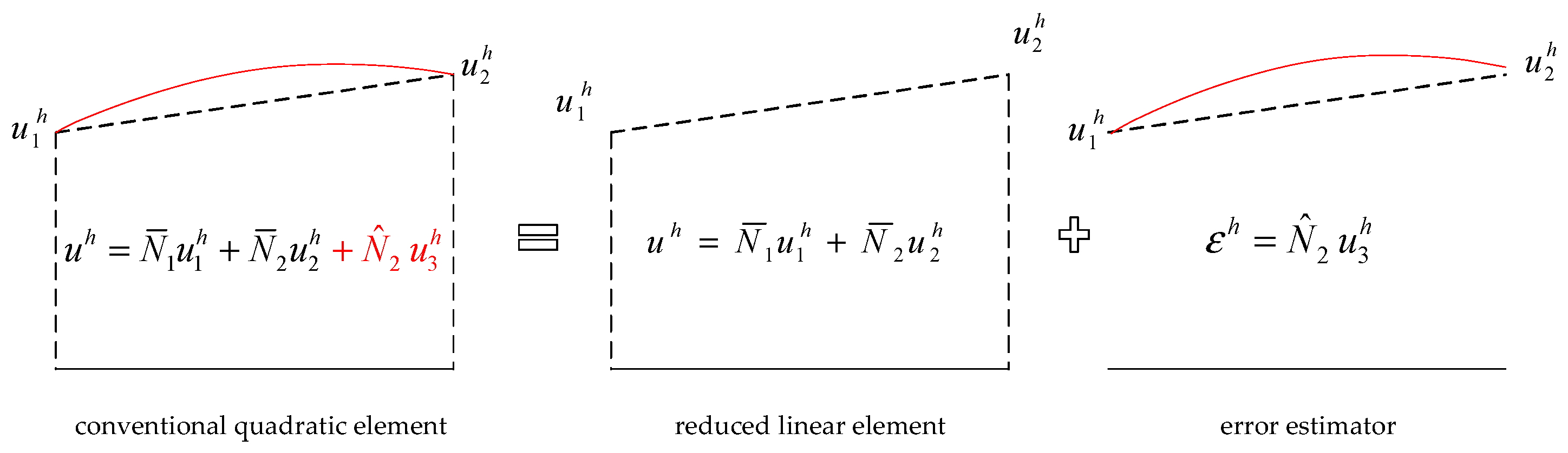
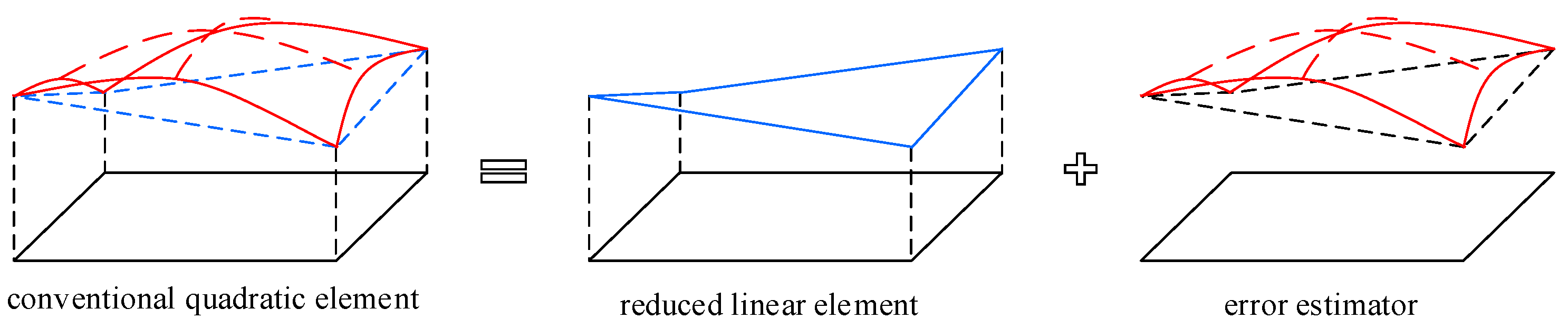
The basic idea of the reduced element is very simple and can be summarized as follows. Supposing the solution for the reduced element of degree
m is sought, a conventional FE analysis is first performed using elements of degree
. After obtaining the full solution
of the conventional elements, the reduced solution
is extracted by retaining terms up to degree
m, while the highest-degree terms (i.e., degree
) serve as a built-in pointwise error estimator
for the reduced solution
. In other words, the solution
of the conventional element is decomposed into two parts
, where
represents a reduced solution and
is an error estimator for the reduced solution
.
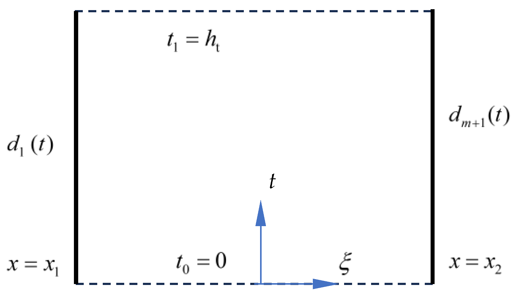
Figure 1 and
Figure 2 illustrate the schematic diagrams of the structures for 1D and 2D reduced linear elements, respectively. By utilizing the “order difference” in accuracy between the full solution and the reduced solution, a built-in error estimator
that can be used for pointwise error estimation is readily available, naturally resulting in a maximum-norm-adaptive algorithm using the reduced solution as the final solution.
The reduced element possesses several advantages, briefly summarized as follows: (1) Unified construction of reduced elements for arbitrary polynomial degrees ; (2) unconditional stability for IVPs across diverse problem types; (3) nodal convergence orders in 1D ordinary differential equations (ODEs) twice those of interior solutions, particularly advantageous for IVPs with long-time domains; (4) nodal accuracy exceeding interior convergence by at least one order, localizing errors to element interiors and significantly improving local refinement reliability; and (5) a built-in maximum norm error estimator enabling adaptive algorithms to meet user-defined error tolerances.
Taking the extended string vibration equation (with damping and an elastic foundation) as the model problem, this paper proposes the space–time reduced element with an effective and reliable adaptive algorithm driven by spatial mesh refinement and time-stepping adjustment controlled by the maximum norm. This paper presents the theoretical analysis and numerical implementation of the space–time reduced elements of degree . To demonstrate the feasibility and effectiveness of this method, several typical numerical examples are presented, covering cases such as initial velocity, initial displacement, abrupt local load, damping, concentrated load, uniform load, and even moving load, for all of which satisfactory results are obtained.
4. Adaptivity Algorithms
4.1. Objective of Adaptivity
The ultimate objective of the adaptive analysis in this paper is to find an optimal mesh, such that the reduced solution
of degree
satisfies the user-specified tolerance
on each element
in the maximum norm:
Since the exact solution
is generally unknown, the full order solution
of degree
is used to replace
for the error checking and then Equation (26) becomes
Note that since the velocity may often be discontinuous or even singular in the temporal dimension for quite a large number of problems, the present algorithm only adaptively controls the errors of the displacement .
Also, before Equation (27) is satisfied on each space–time element, we first require the nodal line displacements to satisfy [
16]
where the lower and upper bounds are simply taken as
, as suggested in Refs. [
16,
19]. We comment that the lower bound
is to avoid redundant accuracy and repeated changes in time-step sizes, and the upper bound
is to allow some room for the computed errors to slightly exceed the preset tolerance
for long time domains. Again, the present algorithm does not impose error controls on the nodal line velocities
. Note that
is not used in calculation of
and hence does not directly affect the accuracy of
.
For convenience, let
and
denote the estimated error ratio and true error ratio defined respectively by
with the corresponding maximum error ratios being
By introducing the definition of error ratios, it is easy to check whether the final solution satisfies the pre-specified accuracy requirement or not. If the final results satisfy
, then the adaptive analysis achieves full success, and according to Refs. [
23,
24], the successful estimated error allows for a 20% fluctuation, which means that, in terms of the error ratio, if
or thereabouts, then the adaptive analysis is also considered to be valid.
4.2. Error Calculations
Although there are
nodal line solutions on an element, the error calculation of Equation (28) is very simple and straightforward
where the maximum value of
can be calculated in advance without the need for pointwise searching, e.g.,
For the error of on the whole space–time element, closed forms of maximum error may not be readily available, and the errors can be calculated numerically at an regular grid point on the element and then the maximum value can be searched for. Usually, each dimension is divided into 12 uniform segments (i.e., ), which is sufficient.
4.3. Treatment of Initial Conditions
For the prescribed initial displacement
, adaptive piecewise polynomial interpolations of degree
are used to obtain such initial condition
that satisfy
To achieve this, starting from an initial coarse mesh provided by the user in the space domain , a piecewise polynomial interpolation is conducted, and then if Equation (33) is violated on any intervals, the interval is divided into two sub-intervals and the process is repeated until Equation (33) is satisfied, as a result of which an initial mesh for the spatial dimension is obtained.
4.4. Mesh Adaptivity
4.4.1. Time-Step Size Adjustment
After each FE run, we first check if the time-step size (element length
) is acceptable. If for any nodal lines in the temporal dimension, Equation (28) is not satisfied, then a new element length is calculated by the formula proposed in Ref. [
16] as follows:
where
is the current element size and
is a safety factor which is set as
in this paper. For the new
, another FE run is carried out and the process is repeated until Equation (28) is satisfied.
For completeness, we give Equation (34) a brief explanation. Suppose with time-step size
, an FE solution
with element degree
is obtained. According to Ref. [
21], the maximum error is bounded
. With Integral Mean Value theorem, we have
. This makes the above equation change to
, from which the constant
can be calculated. Now the new
can be found from the requirement of
, which leads to Equation (34).
4.4.2. Spatial Mesh Refinement
Then we check if the spatial mesh is acceptable. If for any elements on the current time-step, Equation (27) is not satisfied, we simply divide this element into two sub-elements by bisecting so that becomes . After a new mesh is generated in the spatial dimension, another FE run is conducted. The above process is repeated until all elements on the current time-step satisfy the error tolerance pointwisely.
4.5. Hanging Nodes
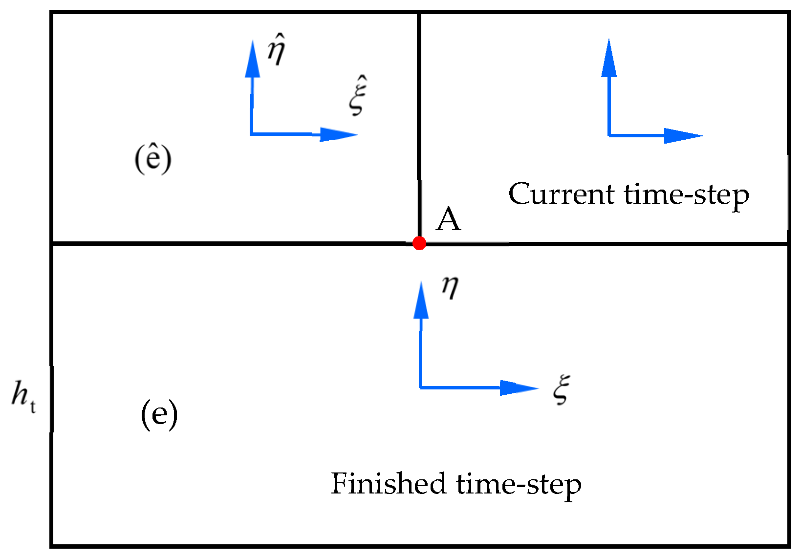
The above mesh adaptivity strategy may generate hanging nodes like point A in
Figure 4. Since the present algorithm is a type of step-by-step integration in time, the FE solution on the upper side of the finished time-step in
Figure 4 is known and serves as the initial conditions (like
and
) for the current time-step. Then the usual piecewise polynomial interpolation of degree
m can be done to keep the conforming property for both the full solution and the reduced solution.
4.6. Backtracking
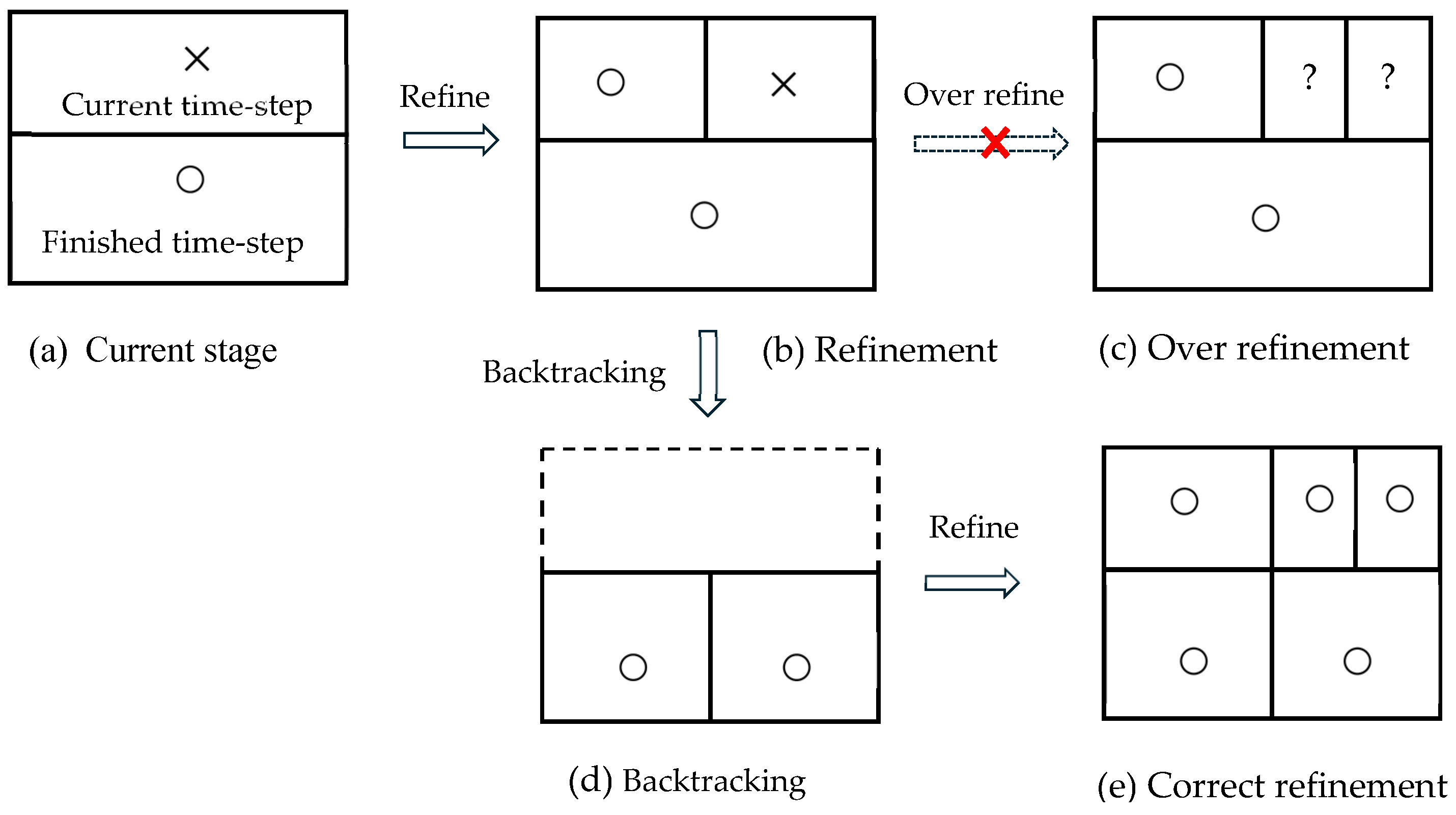
For simplicity and efficiency, at most two hanging elements are allowed to be hung onto a single side of a normal element, otherwise the normal element is to be further bisected into two in a backtracking process. To be more specific, consider the local mesh refinement shown in
Figure 5 where the elements that satisfy the error tolerance are denoted by “O”, or otherwise by “X”.
Figure 5a is the initial mesh where the upper element needs to be refined. Normal refinement leads to the mesh in
Figure 5b, where the upper-right element requires further refinement, which would yield the mesh in
Figure 5c and is not accepted since in that case there will be three hanging elements hanging on a single side of the normal element. Then the algorithm will take a step back to the already finished step, refine the overburden element and then proceed. Although this backtracking process may cause slightly redundant accuracy for the normal element, it provides better initial conditions for the upper elements and meanwhile makes the space–time mesh more structured.
4.7. Adaptivity Algorithm
The adaptivity algorithm for the space–time reduced element approach can be briefly summarized as follows:
Specify tolerance , the degree m of the reduced element;
Generate an initial mesh by adaptive interpolation to
(
Section 4.3) and assign an initial time-step size
;
Generate FEMOL matrices and vector , , and (Equation (10)) using the space element of degree and form the first-order IVP in ODEs (Equation (12));
Solve the first-order ODEs in Equation (12) by the time element of degree
with adaptive time-step sizes until all the nodal line solutions satisfy Equation (28) [
16], and then obtain the full solution
and reduced solution
on each nodal line with a new time-step size
;
For the current time-step, check if each space–time element satisfies Equation (27);
If Equation (27) is satisfied, then move to the next time-step with the current spatial mesh and time-step as the initial mesh and time-step , and then return to Step 3;
If Equation (27) is not satisfied by any elements, bisect them in the spatial dimension and then check whether backtracking is needed;
If backtracking is unnecessary, return to Step 3;
If backtracking is required, return to the previous time-step and return to Step 3;
The above procedure is repeated until reaching the end of the time domain .
Note that the present paper employed the more stringent maximum norm rather than the more commonly used energy norm employed in most adaptive analyses. Numerous numerical experiments show that, in most cases, satisfaction of Equation (27) would indeed make Equation (26) also satisfied.
5. Numerical Examples
In this section, representative numerical examples are given to test the proposed algorithm. The above algorithm has been coded in Fortran 90 and implemented on a PC. In the following, the element degree exclusively refers to the polynomial degree used in the reduced element. In the practical computation, various tolerances ranging from to are adopted, and the linear () to cubic () reduced elements are employed for the presentation although other degreed elements have also been tested. For all the examples, the initial time-step size is taken as .
5.1. An Illustrative Example
This test problem is Example 5.2 in Ref. [
1]. In this example, the first two time-steps of the adaptive procedure are given in detail and then full results from elements of different degrees and different error tolerances are presented. The problem is defined as follows:
with the exact solution being
. The tolerance is set
, and the initial time-step size (time element length) is
. Since the solution is symmetric, only half space domain
is used in computation. The linear reduced elements (
) is used as the final solution and the initial number of elements of the spatial mesh is one. Then from Equation (4), the quadratic trial function of the full element for FEMOL is
The corresponding element matrices and vector of FEMOL in Equation (10) can be derived as
Since the present algorithm imposes error controls on
only, the adaptive interpolation to
proves that a single space element is sufficient and then the initial value vectors are
Introducing the boundary condition, the second-order FEMOL ODEs can be derived
Thus, the first-order ODEs in Equation (12) can be formed. Then the trial function vector and test function vector for the time element are respectively as follows:
Note that the components of
are replaced by the initial values in Equation (38). Following the process described in Ref. [
16], the FE solutions for the nodal displacement vectors are
Without extracting the reduced solution on the nodal lines, the errors can be directly calculated using Equations (31) and (32) as follows:
Thus, by Equation (28), the maximum estimated error ratio for the time element is
and therefore the current time-step size
needs to be adjusted. A new step size is predicted using Equation (34) as follows:
Then repeating the FE process for the time elements with the new
yields a new set of nodal displacement vectors,
and the corresponding estimated maximum error ratio is 0.714, which satisfies the requirement in Equation (28). Therefore, the full solution of the displacement is
Making a linear interpolation to
yields the reduced solution
It is not difficult to find out that the estimated maximum error ratio in the entire space–time element is
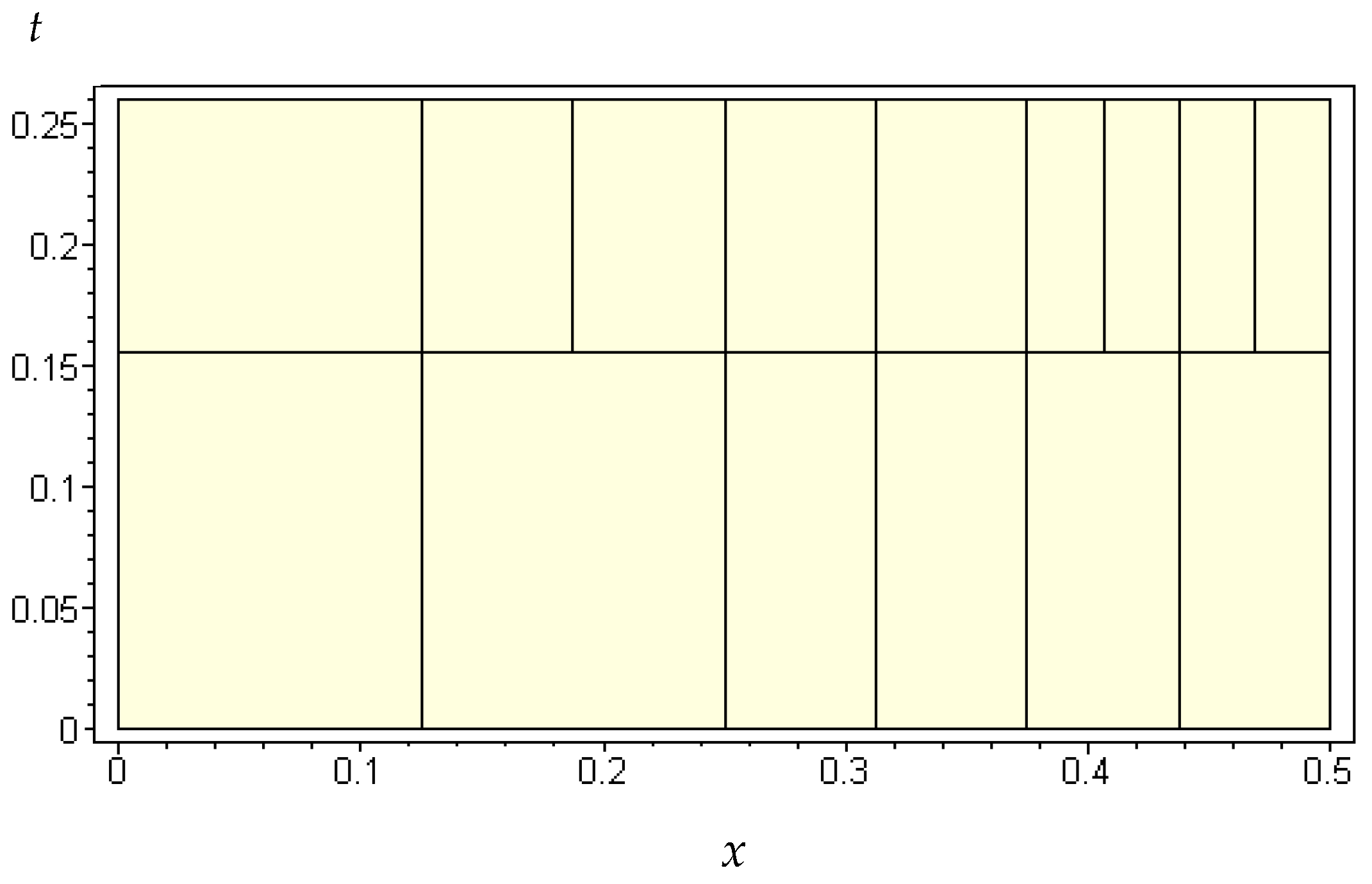
, which fails to meet the error tolerance. Therefore, the element should be divided into two. The subsequent iterative process is summarized in
Table 1 and the finished mesh is shown in
Figure 6.
After finishing the first time-step, we proceed to the second time-step with both the spatial mesh and the time-step size inherited from the first time-step, i.e., six space elements and
. After adaptative process for the time-step size, it is adjusted to
. Then checking each space–time element error shows that the second, fifth and sixth elements exceed the tolerance and need to be bisected, after which a nine-element spatial mesh is generated as shown in
Figure 6. This spatial mesh refinement yields some hanging nodes, which present no difficulties and can be easily treated, as done in the interpolation to the initial values by picking up the corresponding solution values of the upper side of the previous time-step. Another round FE run for the nodal line solutions of the current time-step shows that both the time-step size and the spatial mesh are adequate to meet the error tolerance, with the estimated maximum error ratio
and true maximum error ratio
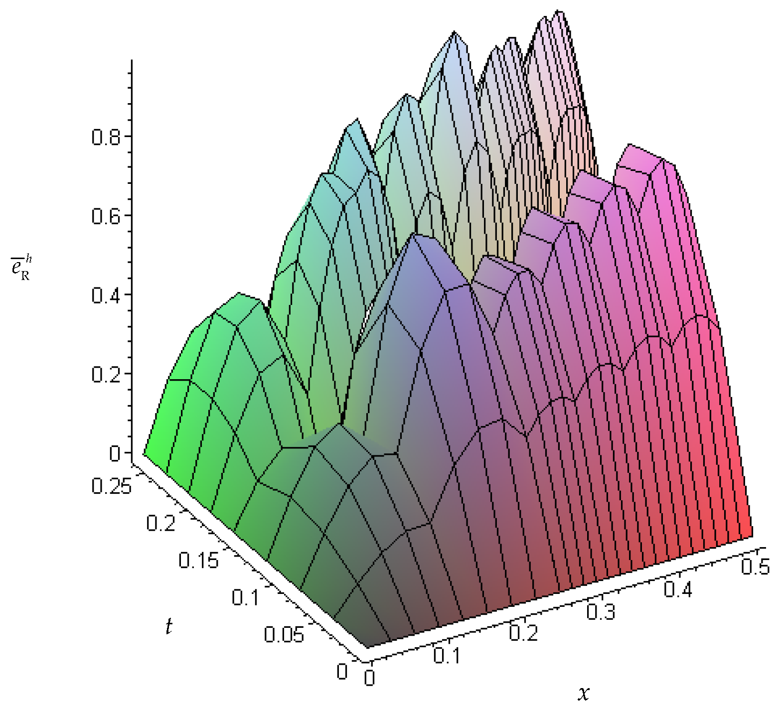
on the second time-step. It is seen that the estimated error is very close to the true error. The distribution of the true error ratio is shown in
Figure 7. Then the adaptive analysis of the second time-step has been successfully fulfilled.
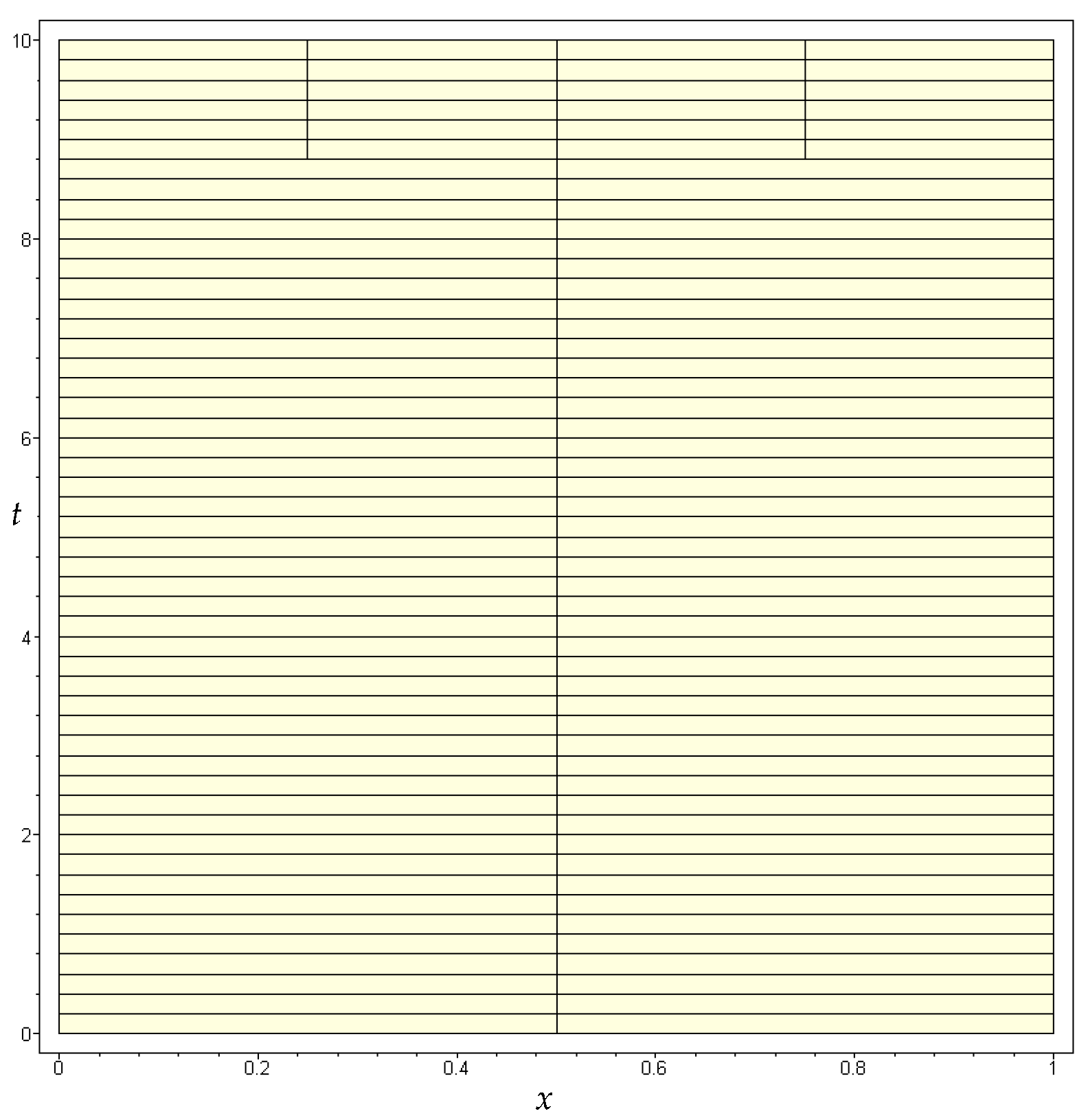
This problem has also been solved on a longer time domain
using elements of different degrees with different error tolerances, and the computed results are shown in
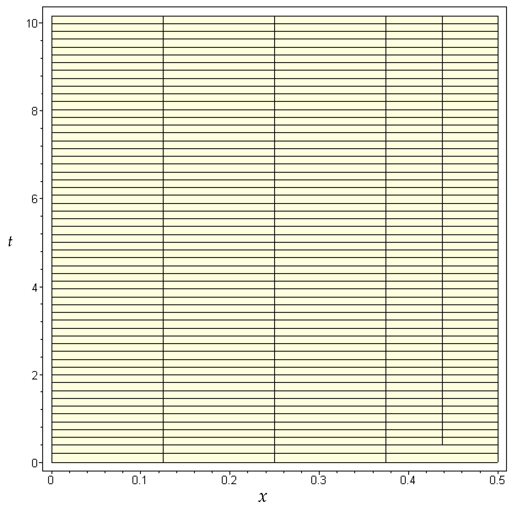
Table 2. The final mesh for
and
is shown in
Figure 8. It is observed that the most adapted FE solutions strictly satisfy the error tolerances, and the overall performance of the proposed algorithm is satisfactory.
5.2. An Acoustic Wave Problem
This test problem is Example 5.1 in Ref. [
1], which is more challenging. The problem is defined as follows:
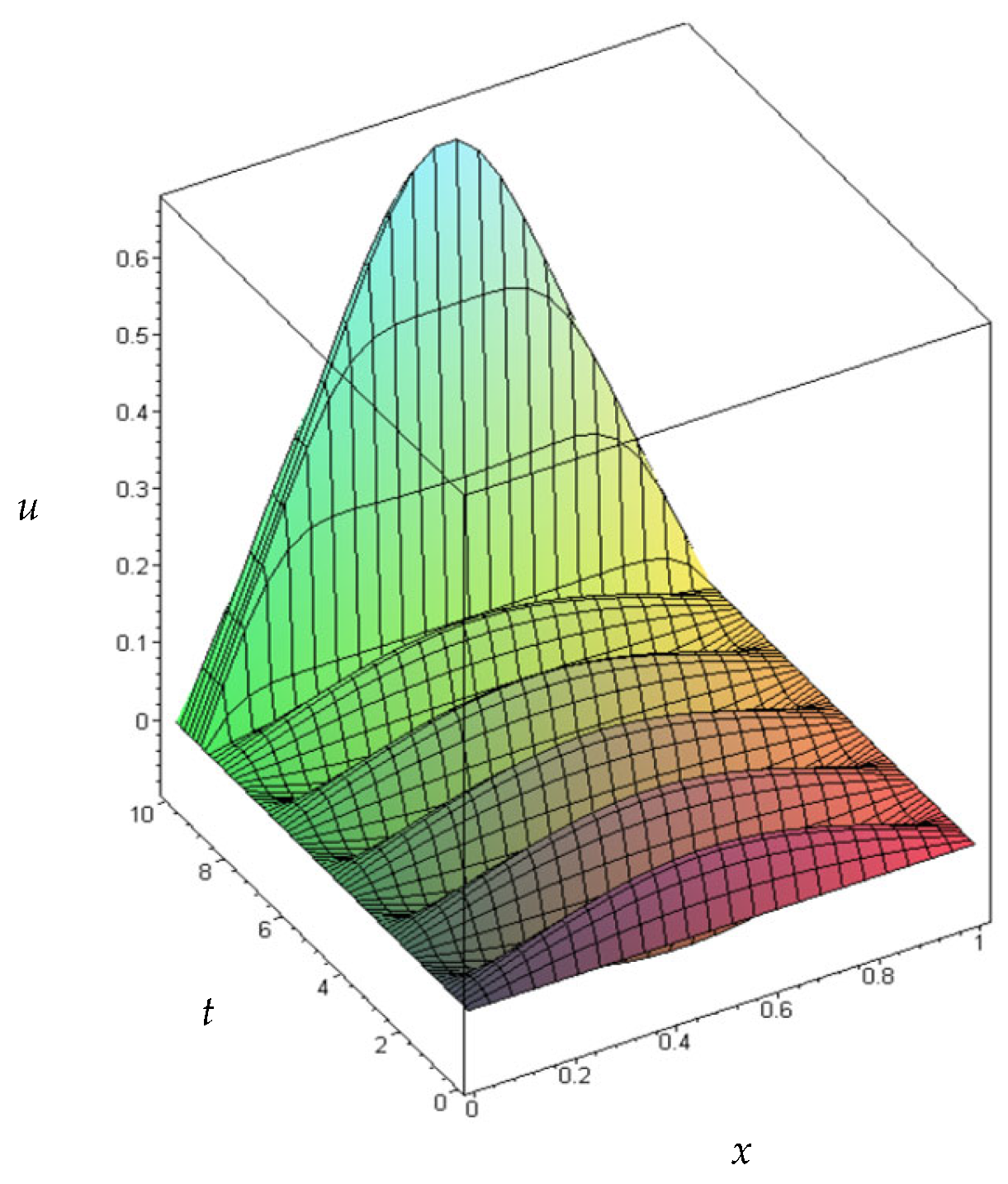
A Fourier series expansion solution of 120 terms is employed to simulate the exact solution for error checking, whose shape is shown in
Figure 9. This problem is computed using reduced elements of degree
and
with error tolerances
and
, respectively. The computed results are shown in
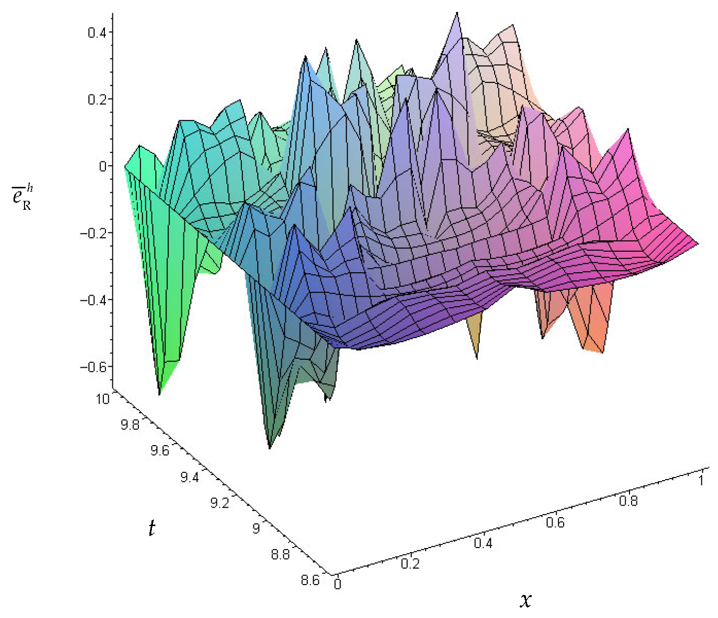
Table 3. For
and
, the true error ratio distribution and the final mesh are shown in
Figure 10 and
Figure 11, respectively. It is seen that most FE solutions meet the error tolerances satisfactorily. For
and
, the true error ratio is not strictly satisfied, for which one of the reasons is that the ‘true’ solution is a series solution, and its accuracy is not sufficient to serve as a true solution for the stringent tolerance
.
5.3. Constant Initial Velocity Problem
This example considers an elastic string with fixed ends excited by an initial velocity
, which is defined as follows:
The string is fixed at two ends where the velocity is equal to zero, i.e., , hence the initial velocity is discontinuous in space at the two ends.
5.3.1. Ten-Term Series Solution as the Objective
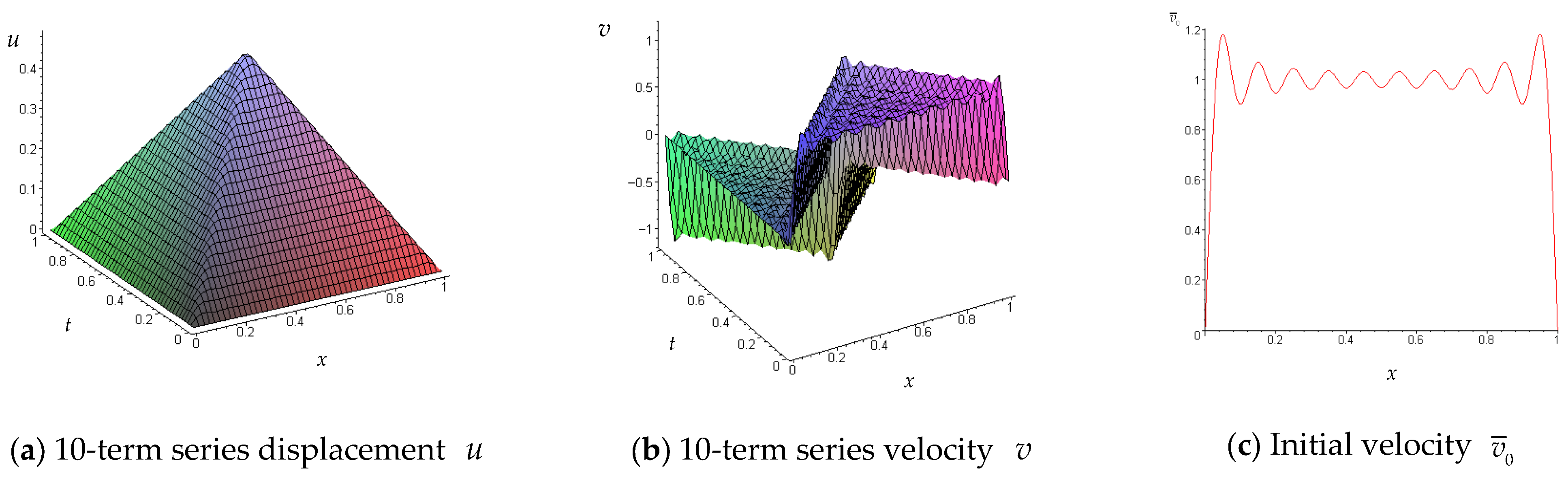
In this case, the 10-term series solution is taken as the exact solution as shown in
Figure 12a,b and the derived initial velocity
is shown in
Figure 12c. This treatment removes the discontinuity of the initial velocity, but the steep variations at the two ends would demand corresponding adaptivity efforts.
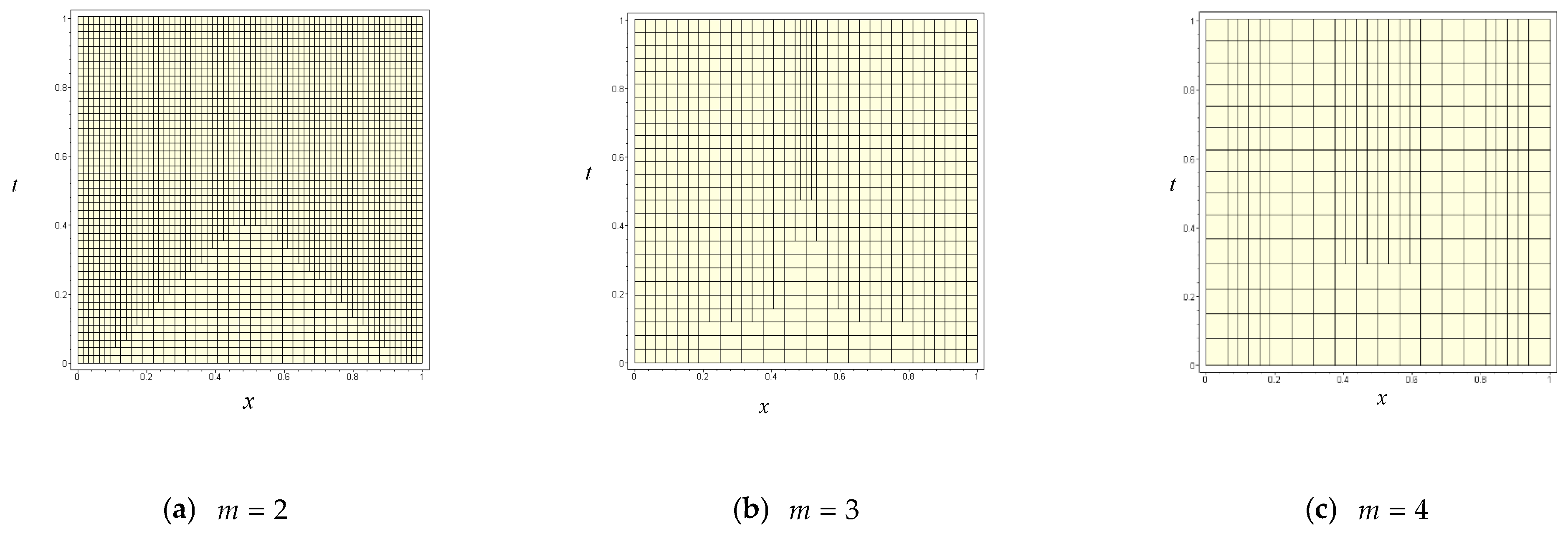
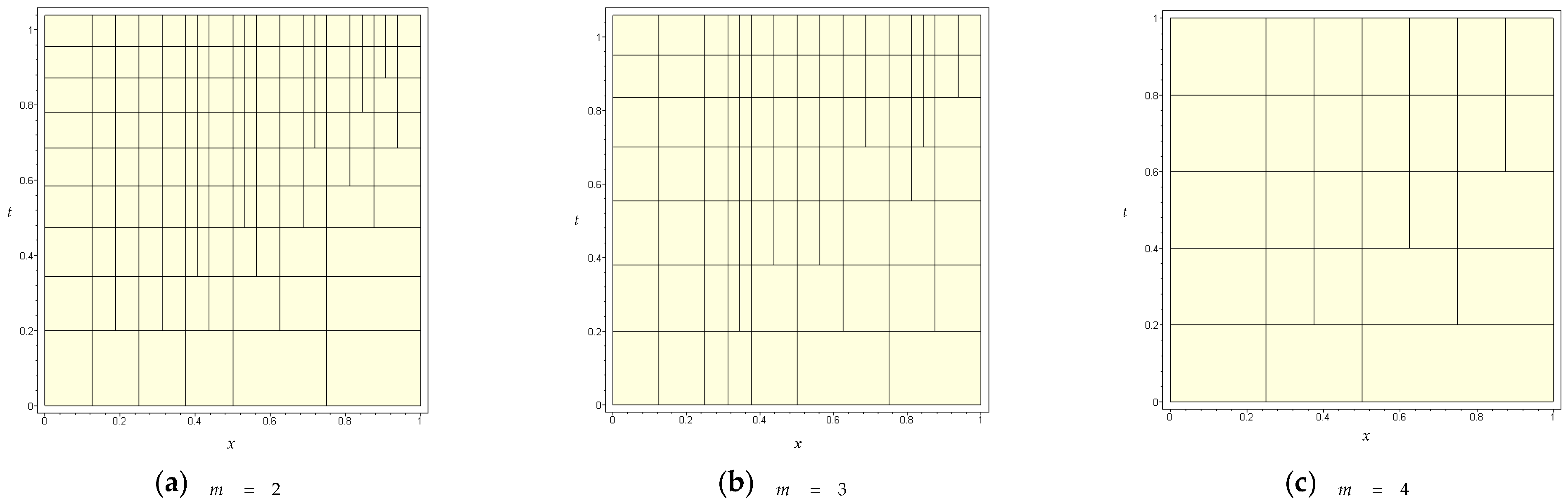
Table 4 gives the computed results of different element degrees and tolerances. For
,
Figure 13 shows the final meshes for elements of different degrees. It is seen that most FE solutions meet the error tolerances satisfactorily.
5.3.2. Piecewise Linear Approximation to Constant Velocity
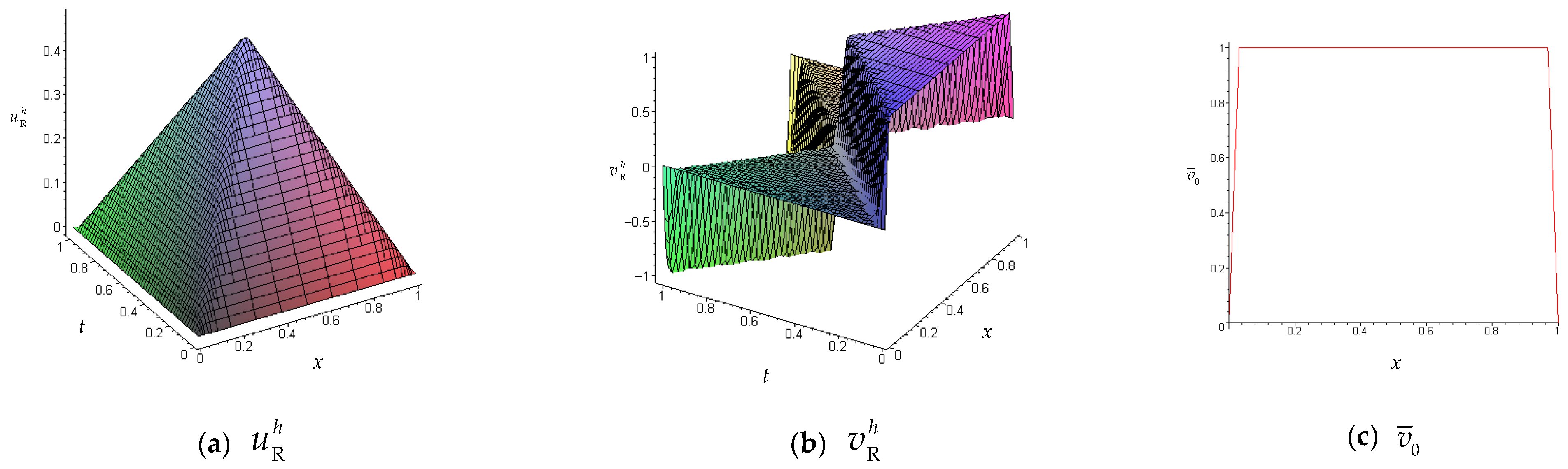
In this case, instead of the series solution, the exact solution is the adaptive objective. However, to remove the discontinuity of the initial velocity, the initial velocity is modeled by a piecewise linear approximation as follows:
as shown in
Figure 14c. Since the exact solution is not available, the true errors cannot be evaluated either. For
, reduced elements of different degrees are taken in computation.
Figure 14a,b shows the reduced solutions of
.
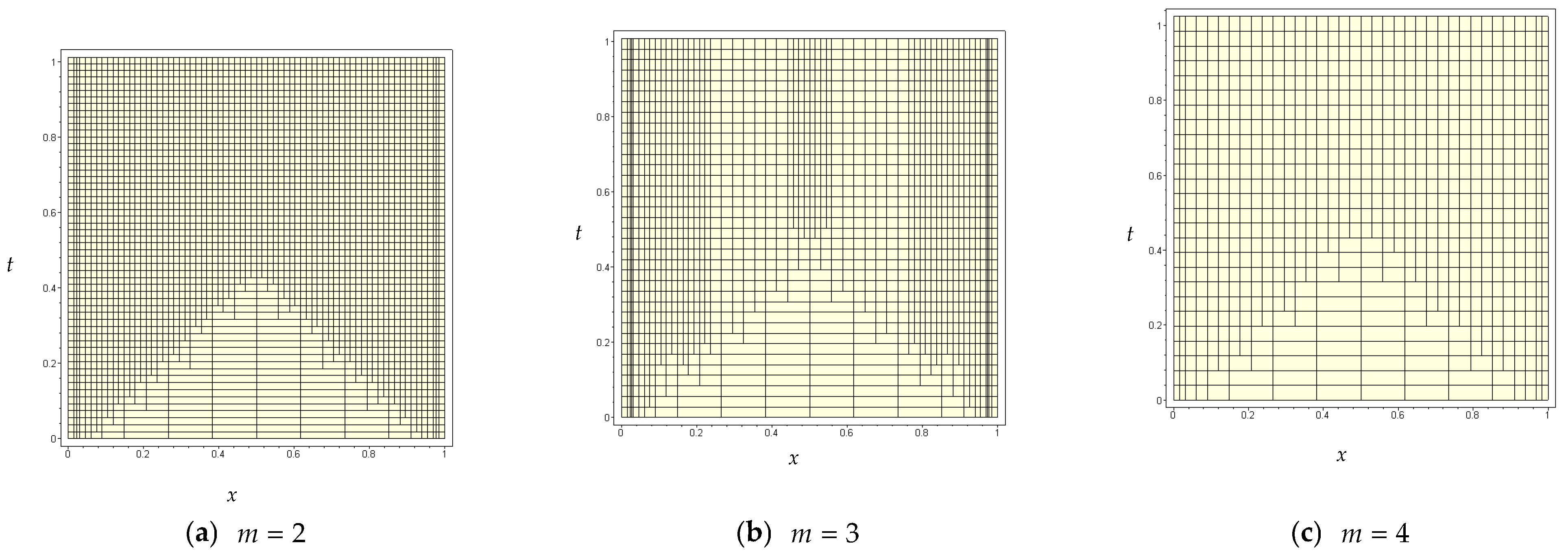
Figure 15 shows the final meshes for the elements of different degrees. It is seen that the reduced solution
and
are smoother than those in Example 5.3.1 and is trusted to be closer to the exact solution.
5.4. Moving Concentrated Load
This example considers an elastic string with fixed ends subjected to a concentrated load
moving from the left end to the right end at a velocity
, which is defined using the Dirac
function as follows:
For simplicity, we set
, for which the exact solution can readily be obtained using the Heaviside function
as follows:
which is shown in
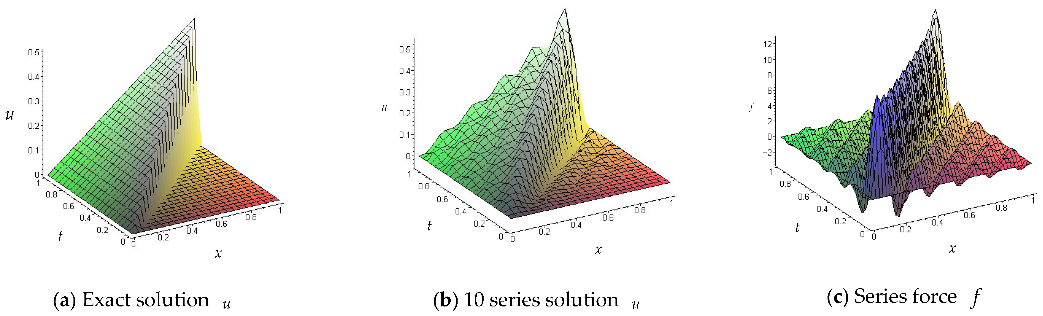
Figure 16a. In this case, the displacement
on the two sides of
is discontinuous and the corresponding velocity is singular.
5.4.1. Ten-Term Series Solution as the Objective
In this case, the 10-term series solution is taken as the exact solution as shown in
Figure 14b and the load term
is derived from the specified solution as shown in
Figure 14c.
Table 5 gives the computed results of different element degrees and tolerances. For
,
Figure 17 shows the final meshes for elements of different degrees. It is seen that most FE solutions meet the error tolerances satisfactorily.
5.4.2. Direct Concentrated Load
In this case, instead of the series solution, the exact solution is the adaptive objective with the concentrated load directly applied at the appropriate position.
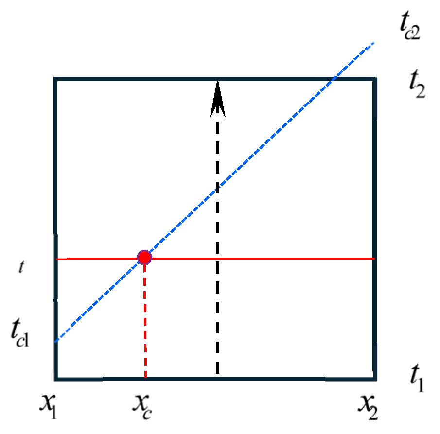
Figure 18 shows an illustrative example of the moving load
passing a typical element. Suppose the load
is at
for the time
. For the particular time
, the equivalent nodal line load vector
in Equation (10) can be calculated using spatial coordinate
as
To transform the above formula into a function of time
, note that
,
and
. Then when
, there is no load on the time interval
, and when
, there is no load on
either. Therefore, to keep the lower and upper bounds
and
unchanged for the current time-step,
can be calculated as follows:
For
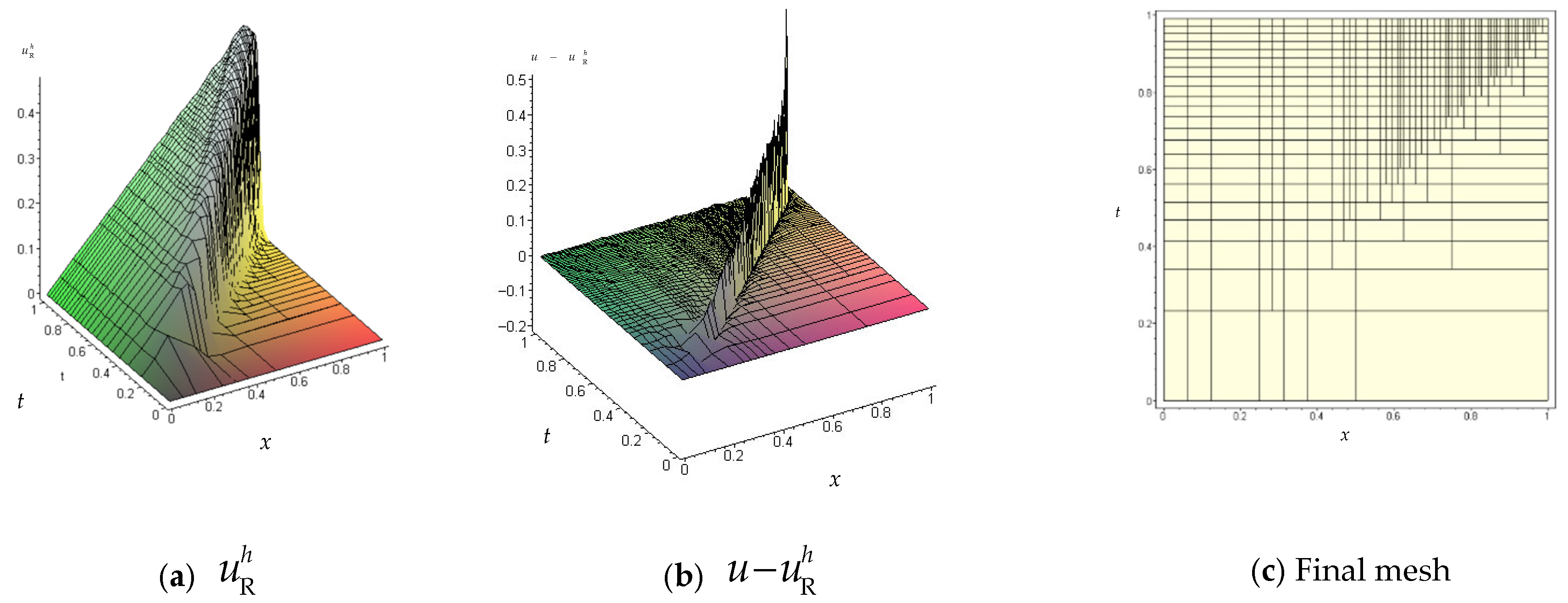
, reduced elements of different degrees are taken in computation.
Figure 19 shows the reduced solutions of
and final mesh. It is seen that the adapted mesh is reasonably refined and the reduced solution
and
are smoother on plane surfaces than those in Example 5.4.1 with the large errors mainly located along the discontinuous diagonal line.
5.5. Vibration with Damping and an Elastic Foundation
This example considers an elastic string with fixed ends subjected to a sudden uniform load
with damping
and an elastic foundation
, which is defined as follows:
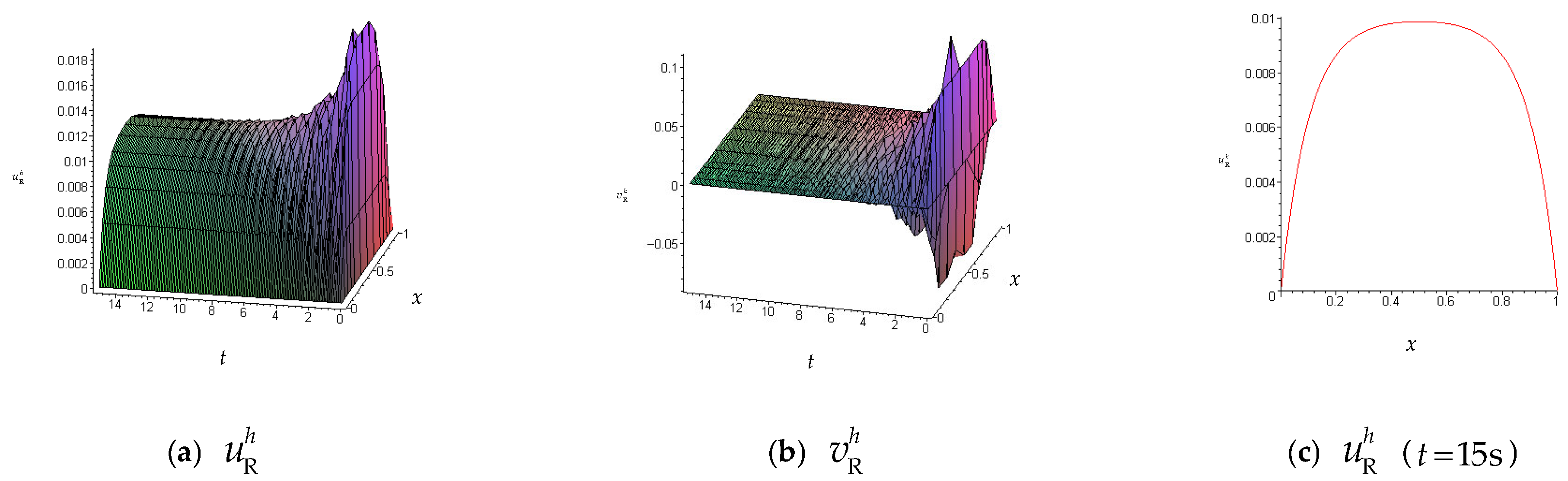
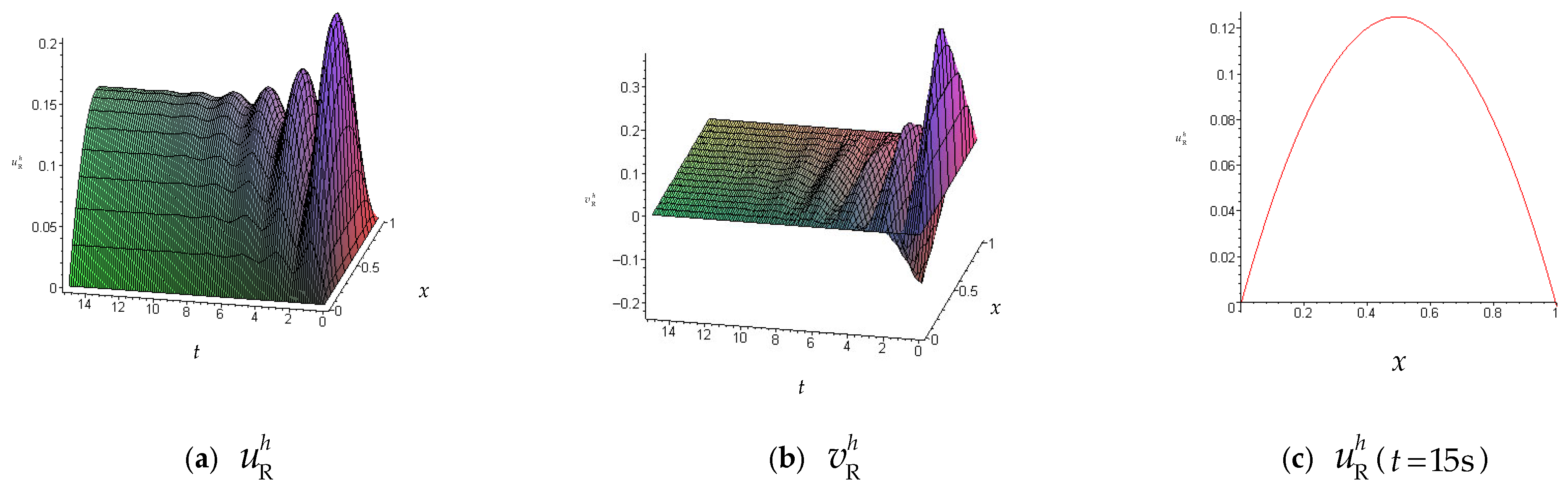
The quadratic reduced element () is used with . Since there is no exact solution available, a long time domain of is deliberately chosen so that a steady state can be achieved at the terminal time, which can be compared with the computed result.
5.5.1. Vibration with Damping Alone
In this case,
and
are taken in computation.
Figure 20 shows the adapted reduced solutions of displacement, velocity on the space–time domain and the displacement at the end time. As a check, the computed displacement at the mid-span at the terminal time is 0.125029, which is very close to the exact steady state value
.
5.5.2. Vibration with Both Damping and an Elastic Foundation
In this case,
and
are taken in computation.
Figure 21 shows the adapted reduced solutions of displacement, velocity on the space–time domain and the displacement at the terminal time. As a check, the computed displacement at the mid-span at the terminal time is 0.009870, which is very close to the exact steady-state value 0.009865.