A Privacy-Preserving Classification Framework for Multi-Class Imbalanced Data Using Geometric Oversampling and Homomorphic Encryption

Abstract

Data classification tasks based on deep neural networks and machine learning are increasingly used in different fields, such as medicine, finance, and data circulation. However, in these applications, the accuracy of predictions must be guaranteed, and the privacy and security of prediction data and models must be guaranteed. In an unsafe cloud environment, cloud users are reluctant to use the classification prediction tasks provided by the cloud. To solve these problems, this paper researches the data oversampling method and proposes the G-MSMOTE method, which can solve the oversampling problem of multiple minority classes in the data set, generate more diverse data, and solve the data imbalance problem. By improving the traditional FV and using CRT technology to improve coding efficiency, the cloud receives the user’s encrypted ciphertext, and the neural network completes the data prediction task in the ciphertext, thereby providing confidentiality for user data and model parameters under the semi-honest adversarial model, assuming the security of the underlying fully homomorphic encryption scheme and accepting the leakage of model architecture and ciphertext sizes. The feasibility of our method was demonstrated through experimental comparative analysis. We created unbalanced cases based on the MNIST dataset and performed comparative analysis in plain and ciphertext. In the balanced dataset, the model’s prediction accuracy in ciphertext reached 93.44%. In the unbalanced case, after preprocessing with our improved G-MSMOTE algorithm, the model’s prediction accuracy in ciphertext increased by at least 10%. These results show that our scheme can efficiently, accurately, and securely (under the semi-honest model) complete the data classification prediction task.

1. Introduction

With the development of technologies such as cloud computing and big data, a large amount of data has provided an excellent environment for the development of artificial intelligence, making artificial intelligence technology based on deep learning a current research hotspot. This technology has achieved remarkable results and is widely used in various fields, such as traffic analysis, spam detection, intrusion detection, auxiliary medical detection, face recognition, and highway engineering. In addition, as the model’s functionality and accuracy gradually improve, it is difficult to deploy the model on the user side. Therefore, it is necessary to perform training and deploy deep learning models on cloud servers. Through machine learning as a service (MLaaS), users can use the models in the cloud server to achieve predictive reasoning, and users do not need to worry about maintaining models and services during this process.

However, the use of models for prediction and inference typically requires access to the original plaintext data. Performing such tasks on untrusted or honest-but-curious servers may lead to the leakage of private data, posing significant security and privacy risks. These risks apply to a wide range of machine learning models, including linear regression [1], linear classifiers [2], decision trees [3], and neural networks [4,5,6]. Although some existing approaches, such as the CryptoNets [7] and CryptoDL [8] models, incorporate data security measures, they do not adequately address the issue of data imbalance.

Most of the real-world datasets are inherently imbalanced [9]. It is difficult for classifiers to learn features from small class samples, which reduces the availability of cloud services. Imbalanced data is a pattern classification problem. In recent years, many researchers and professionals have conducted in-depth research on this problem and have alleviated or mitigated the imbalanced data problem to varying degrees [10,11,12,13]. However, the problem still needs to be solved entirely. To sum up, the main problems in data classification tasks are as follows:

• Generate duplicate instances and noisy data in the imbalanced data oversampling scheme. In an imbalanced dataset, data of other categories are organized in clusters, with complex decision boundaries between categories. In this case, the K value in the oversampling scheme is difficult to set. A smaller K value will reduce the probability of noise generation but produce more repeated data. This also leads to a lack of data diversity, which causes the model to overfit. If the K value is selected to be larger, more noise samples will be generated, blurring the category boundaries between the data. Therefore, increasing the diversity of new synthetic data and expanding the data generation process is necessary [14].
• There are security issues when using cloud servers for reasoning. Doctors use cloud services to analyze and diagnose patients’ CT images in the actual medical diagnosis process [15,16]. Since this process involves private patient information, traditional hospitals use encryption technology to ensure the security of the data transmission process. However, when the cloud server performs inference and prediction, it decrypts the data, directly infers the plaintext data, encrypts the inference results, and returns them to the doctor.

In this work, we address the multi-class imbalanced data classification problem, where a dataset contains more than two target classes (e.g., digits 0–9 in MNIST), and the class frequencies are highly skewed. Our solution involves an oversampling scheme designed for such multi-category data, meaning it can generate synthetic samples for multiple minority classes within a single dataset. Furthermore, to achieve practical efficiency in homomorphic encryption, our implementation leverages batch processing (or ciphertext packing), a technique that encodes multiple data points into a single ciphertext polynomial to perform Single Instruction, Multiple Data (SIMD) operations.

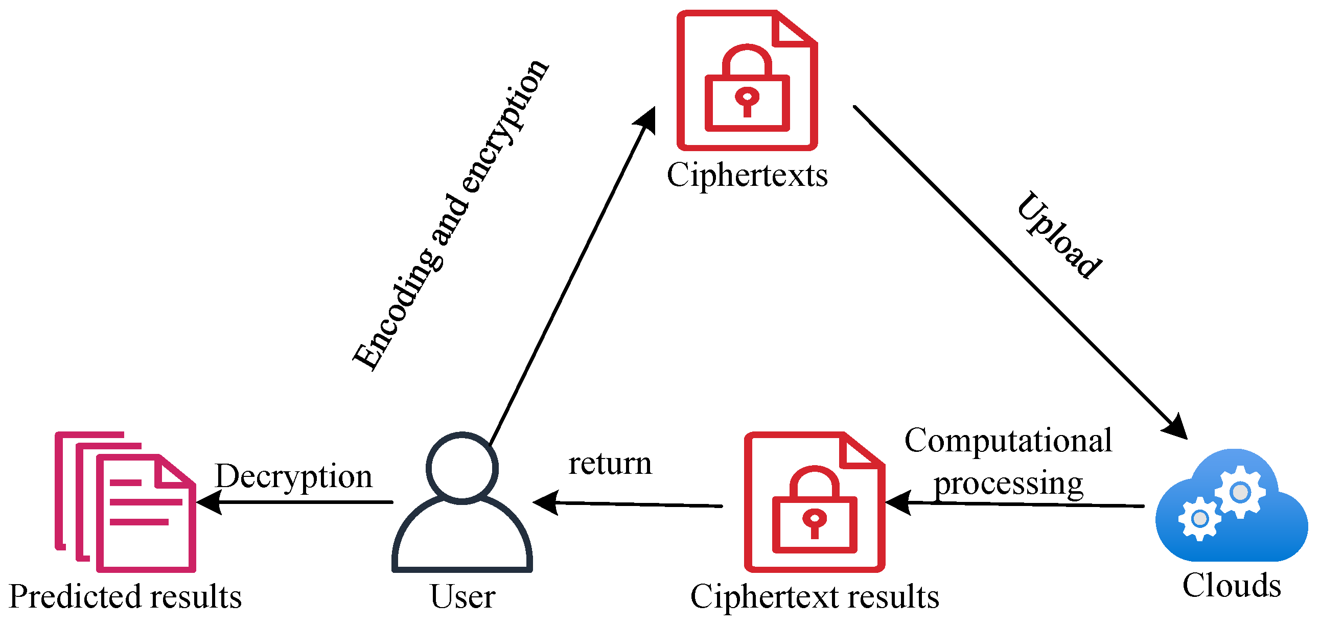
To overcome the poor model prediction effect caused by unbalanced data and the problem of data privacy leakage in the prediction process, we combined CryptoNets and data oversampling methods. We proposed a G-MSMOTE scheme based on CryptoNets. In processing unbalanced datasets, the data generation mechanism is replaced by defining flexible geometric regions around each minority class sample point. Then, new synthetic samples are generated within the boundaries of each area. Algorithm parameters control the synthesis of new samples. To improve the training effect of the model, we modify the model so that the model is trained under the plaintext dataset. When making predictions, the prediction of ciphertext data is completed without changing the model structure. The main idea of ciphertext prediction is shown in Figure 1.

To clarify the security model and privacy goals, our scheme considers a semi-honest (honest-but-curious) cloud server. The server follows the protocol but may attempt to infer information from the encrypted data and intermediate results. We aim to achieve two privacy goals: (1) client input confidentiality, ensuring the server cannot access the user’s plaintext data; and (2) model parameter confidentiality, keeping the server’s model parameters private from the user. The design ensures that the server performs computations only on encrypted data without decrypting it, protecting both user data and the server’s intellectual property. Our security analysis (Section 5) follows standard FHE inference threat models, where the neural network architecture and ciphertext sizes are considered non-sensitive information that may be leaked.

To solve the problem of imbalanced data classification and privacy data leakage during model prediction, the main work of this paper is as follows:

• We designed an imbalanced data oversampling scheme, the Geometric Multi-class Synthetic Minority Oversampling Technique (G-MSMOTE), which generalizes the G-SMOTE framework to multi-category data. It operates iteratively on each minority class, using a flexible neighbor selection strategy that considers instances from all classes to generate synthetic samples within a defined geometric region, thereby adapting to complex multi-class decision boundaries.
• Improve CryptoNets to complete the training of plaintext datasets and the prediction of ciphertext data without changing the model structure.
• Improve the FV algorithm to increase the amount of information carried by a single polynomial and improve computational efficiency. Decompose the parameter q to reduce the generated noise.
• Conduct relevant experiments and prove the superiority of the proposed scheme through time and accuracy.

This work presents a system integration framework that couples geometric oversampling with privacy-preserving inference, addressing both data imbalance and data privacy concerns in a unified manner. Our primary contribution is methodological: showing how imbalance-aware preprocessing can be integrated with homomorphic encryption for secure classification under the semi-honest threat model. While we demonstrate the approach on the MNIST benchmark, we acknowledge that clinical application would require further validation on medical datasets and a consideration of domain-specific constraints, as discussed in Section 6. The security of our scheme relies on the well-established CPA-security of the underlying FHE scheme (BFV/SEAL) with explicitly defined leakage, aligning with standard threat models for privacy-preserving ML inference.

This paper structure is as follows. Section 2 analyzes the problem of unbalanced data and the security issues of model prediction in cloud services. Section 3 introduces the improved G-MSMOTE scheme, FV algorithm, and neural network model results in this paper. Section 4 presents the relevant experiments in detail and discusses the results. To verify the security of our proposed solution, we conducted correctness and security analysis; the discussion of the solution is in Section 5. Finally, we have a summary discussion.

2. Related Work

This section reviews the imbalance problem and privacy issue in data classification. The imbalance problem mainly analyzes the research on sampling algorithms, and the data privacy problem analyzes and discusses the related homomorphic encryption methods and neural networks that can operate on the ciphertext.

2.1. Data Imbalance Problem

Traditional methods to solve the data imbalance problem include oversampling, undersampling, mixed sampling, cost-sensitive methods, metadata learning methods, etc. The data sampling method belongs to the data preprocessing process. In contrast, the cost-sensitive and metadata learning methods adjust the model and data during the data training process. Therefore, these data training methods do not apply to ciphertext neural networks. Data sampling method can be used in ciphertext neural networks and can enhance the neural network’s performance without changing the structure of the ciphertext neural network. Undersampling methods remove information from the data, thereby reducing the training effect of the model. Oversampling methods synthesize based on minority class data, increase the amount of data, and reduce the imbalance ratio of the dataset. Therefore, oversampling methods are the most promising solution.

SMOTE [17] is the first oversampling method proposed. It effectively solves the shortcomings of the undersampling method. However, the synthetic samples of this method have high similarity: the K value is fixed, the samples are not diverse, and the synthetic data contains noise. To address these problems, relevant researchers have proposed improvement methods. Based on the idea of data boundaries, Article [18] proposed the Borderline-SMOTE scheme. Synthesizing samples near the data boundary makes it easy to generate noisy data and blurs the data boundary. Article [19] proposed the SMOTE-D scheme, which determines the number of data to be synthesized around each data through the k-nearest neighbour distance between the data. This scheme can evenly synthesize minority class data but will generate too many similar samples, causing the classifier to overfit. To solve the noise and data boundary problems, Article [20] proposed the A-SMOTE scheme, which synthesizes minority class data based on the distance between minority class data, effectively reducing the interference of majority class data in minority class areas and reducing the generation of noise data. The above improved methods are all based on traditional data distance and k-nearest neighbor synthetic data. The generated data quality is low and the data features are not representative. Article [21] proposed DeepSMOTE based on the GAN network. They continuously optimized the generated data through the adversarial network, increased the features in the data, and made the synthetic data more realistic. Due to the disorder of data distribution, some noise samples are difficult to identify. To solve this problem, Article [22] identified the overall data distribution based on the probability density function. They synthesized new data from a global perspective, which effectively reduced the generation of noise data and made the distribution of synthesized data more uniform.

2.2. Data Privacy Problem

Data privacy issues include the privacy of training datasets, the confidentiality of prediction data, and the privacy of model parameters. This article focuses on the privacy of prediction data and model parameters. The method to ensure the confidentiality of prediction data is homomorphic encryption technology, which can realize the calculation of ciphertext data. In order to protect model parameters, the model is stored in the cloud server, which is only visible and available to the server but not to the user.

Homomorphic encryption (HE) was first proposed by [23]; it makes data available but invisible, effectively ensuring data security. Article [7] designed CryptoNets based on the YASHE [24] scheme, which enables the training of plaintext data and inference calculations on ciphertext data. But the network has only five layers, making it difficult to extract and mine data features deeply. Article [25] added a batch normalization layer to CryptoNets by approximating the ReLU activation function with a polynomial [26], making the network structure reach six layers. The training data of CryptoNets uses a CPU, which is very costly. Article [27] designed a CNNS network that can be accelerated by GPU through BFV [28], reducing the computational cost. Since Dowlin et al.’s method calculates each pixel as a ciphertext during encryption, the performance is reduced. Article [29] proposed an FHE matrix multiplication method that uses the image as a unit and encrypts the entire image into a ciphertext, achieving good performance.

Recent Advances and Future Directions in FHE for PPML: While our work builds upon second-generation FHE schemes (B/FV, CKKS) as implemented in libraries like Microsoft SEAL, we acknowledge the rapid evolution of FHE technology through four generations. The latest advancements focus on improving practical efficiency through various approaches:

• Hardware–Software Co-optimization: Recent research demonstrates that specialized hardware accelerators (FPGAs, ASICs, and GPUs) can dramatically improve FHE performance. For instance, the F1 accelerator [30] and the CraterLake architecture [31] show orders-of-magnitude speedup for FHE operations through hardware– software codesign.
• Algorithmic Improvements: Third-generation (Gentry–Sahai–Waters) and fourth-generation (CKKS with bootstrapping optimizations) schemes provide better noise management and support for approximate arithmetic, enabling more complex computations.
• Comprehensive Benchmarking: Recent testbed evaluations of open-source FHE libraries (SEAL, HElib, PALISADE, Lattigo) provide quantitative comparisons of their performance characteristics for PPML workloads [32,33]. These benchmarks help researchers to select appropriate FHE parameters and implementations.
• Application-Specific Optimizations: For PPML specifically, research has focused on optimizing FHE for neural network operations through techniques like polynomial approximations of activation functions, ciphertext packing strategies, and model architecture adaptations.

Our work adopts the BFV scheme from the second generation due to its balance of security, maturity, and availability in production-ready libraries. However, we recognize that future improvements in FHE efficiency will come from both algorithmic advances and dedicated hardware acceleration, which will be crucial for making privacy-preserving machine learning practical for larger-scale applications. Our system architecture is designed to be modular, allowing integration with newer FHE schemes and hardware accelerators as they become available.

3. Our Schemes

The Geometric Synthetic Minority Oversampling Technique (G-SMOTE) is an advanced oversampling method that defines a geometric region around a selected minority class instance and generates synthetic samples within a truncated hyper-spheroid [34]. This approach reduces the generation of noisy samples and increases the diversity of synthetic data compared to the linear interpolation of SMOTE. However, a primary limitation of G-SMOTE is that it is designed for binary classification problems.

To address multi-class imbalanced datasets, we propose an extension named Geometric Multi-class Synthetic Minority Oversampling Technique (G-MSMOTE). The core innovation of G-MSMOTE lies in its generalization of G-SMOTE’s geometric generation mechanism to the multi-class scenario. It operates on a per-minority-class basis, where, for each targeted minority class, the algorithm selects a center instance and a nearest neighbor that can belong to any class (including other minority or majority classes), according to a flexible selection strategy. This allows G-MSMOTE to effectively model the broader data distribution and generate more representative synthetic samples for each minority class in a multi-class environment.

In this chapter, we mainly introduce the imbalanced data scheme based on CryptoNets. Section 3.1 introduces our improved G-SMOTE algorithm in detail; Section 3.2 introduces the structural principle of the neural network model; Section 3.3 presents the data encoding and operation methods; and, finally, Section 3.4 introduces the improved FV scheme.

3.1. Improved G-SMOTE Scheme

Since the SMOTE algorithm easily generates noisy samples and the generated data lacks diversity, Article [34] proposed the G-SMOTE algorithm, which effectively reduces the generation of noisy data by defining a geometric region around each selected minority class sample and performing random interpolation within this region. By setting different initial data selection strategies, the nearest neighbor data is no longer limited to the minority class, thereby improving the diversity of generated data. However, this algorithm also has certain limitations. It only considers two categories, namely, the majority class and the minority class. However, in actual situations, datasets usually have multiple categories. To address this limitation, we improve G-SMOTE, which we call G-MSMOTE in this article. The specific improvements and designs of the scheme are described as follows.

The G-MSMOTE algorithm is designed to handle datasets with m classes (i.e., $S=\{S_1,S_2,\dots ,S_m\}$). It does not perform a single global balancing but instead processes each minority class iteratively. For a target minority class $S_n$, the algorithm synthesizes samples by considering the geometric distribution of instances from all classes, which is a key distinction from binary oversamplers like G-SMOTE. This approach prevents the generation of noisy samples in regions dominated by other classes and is suitable for multi-category data where simple interpolation between two minority-class instances could be harmful.

Suppose the dataset $\mathrm{S}=\{{\mathrm{S}}_1,{\mathrm{S}}_2,\dots ,{\mathrm{S}}_{\mathrm{m}}\}$ has m categories, and the label is $\mathrm{T}=\{{\mathrm{T}}_1,{\mathrm{T}}_2,\dots ,{\mathrm{T}}_{\mathrm{m}}\}$. $S_n$ is one of the minority classes, with the label $T_n$. Set an empty set E to store the newly generated data and generate data according to the following steps:

• Randomly select a sample $x_c$ from $S_n$ as the center of the geometric region for this class.
• Multi-Category Neighbor Selection:
  Select the nearest neighbor sample $x_k$ of $x_c$. The neighbor $x_k$ is found from the entire training set S based on a distance metric, which means it can belong to the target minority class $S_n$ or any other majority or minority class. The specific selection is governed by the strategy parameter ${\alpha }_{sel}$, the number of neighbors k, and the local distribution of the center sample $x_c$. This step enables G-MSMOTE to perceive the global structure of multi-category datasets.
  • ${\alpha }_{sel}=S_n$: The selection strategy is the same as that of the SMOTE scheme. Identify the k nearest neighbors of $x_c$ in the dataset $S_n$ and select one of them as $x_k$. The time complexity of this nearest neighbor selection strategy increases with the dimension of the input space and the parameter k. Therefore, limiting the search to this type of dataset can reduce the computational cost.
  • ${\alpha }_{sel}=S-S_n$: If ${\alpha }_{sel}$ only selects samples in $S_n$, the generated samples may be located in the geometric area of other categories, resulting in the generation of noise. The nearest neighbor samples selected from other classes can eliminate this situation. The $x_k$ from other class samples is chosen as the closest neighbor sample of $x_c$. Therefore, when randomly generating samples within the central sample $x_c$ and the hypersphere with radius $R=\Vert {\mathbf{x}}_c-{\mathbf{x}}_{\kappa }\Vert$, the distance between $x_k$ and $x_c$ can be limited to less than or equal to the distance between $x_c$ and any sample in other classes. This selection strategy loses part of the information of those few categories and also expands the geometric region of the category, which may be noisy.
  • ${\alpha }_{sel}=S$: The nearest neighbor samples of $x_c$ are selected from the entire dataset. They can be samples of the category to which $x_c$ belongs or samples of other categories. The main purpose is to minimize the distance between them and $x_c$. This can ensure that the generated samples are within the control range, thereby avoiding the generation of noise samples. Compared with the other two methods, expanding the minority class sample area is not only safe but also can be further restricted by the minority class samples. The main disadvantage of this method is the high computational cost.

The last step is to generate samples. The center of the unit hypersphere is $x_c=0$, and the radius is $R=1$. Generate a vector $\nu \leftarrow ({\nu }_1,\dots ,{\nu }_p)$ of p random numbers from the normal distribution $N(0,1)$ and calculate the unit vector $e_s={\displaystyle \frac{v}{\left|\nu \right|}}$ in the hypersphere. Generate a random vector $x_g\leftarrow r^{1/p}{e}_s$ in the unit hypersphere using standard distribution and uniform distribution, where r is a random number from the uniform distribution $U(0,1)$. Suppose unit vector $e_{//}={\displaystyle \frac{x_s-x_c}{\mid x_s-x_c\mid }}$, projects $x_g$ onto $e_{//}$ and expresses it as $x_{//}=x_g·e_{//}$ and normalize $x_{//}$ to get $x_{//}=x_{//}{e}_{//}$; then, the orthogonal component $x_{\perp }$ of $x_g$ in the $e_{//}$ direction is obtained by subtracting the component in the $e_{//}$ direction from $x_g$.

The generated vector $x_g$ is truncated according to the truncation function to keep the data within a specific range, thereby avoiding abnormal data points in the predetermined range. Under $x_s\ne x_c$, if $\mid {\alpha }_t-x_{//}\mid >1$, $x_g$ is truncated to $x_g\leftarrow x_g-2x_{//}$, where $x_s$ is a point on the hypersphere’s surface and ${\alpha }_t\in [-1,1]$ is the truncation factor.

Next, we need to deform $x_g$ through the deformation function to increase the diversity of samples. More concretely, the point $x_g$ is moved in a perpendicular direction to the unit vector $e_{//}$, towards the parallel to $e_{//}$ diameter. The hyperparameter ${\alpha }_d\in (0,1]$ controls this deformed mapping, and $x_g$ is adjusted to the new position according to the parameter ${\alpha }_d$. If $x_c$ is not equal to $x_s$, then $x_s$ is deformed, and the deformation process is $x_g\leftarrow x_g-{\alpha }_d{x}_{\perp }$.

Finally, by translating the data vector $x_g$, we can obtain the final $x_{n}ew$. The main purpose of translation is to make the generated data better adapt to the training of the model. $x_g$ is scaled and translated based on the hypersphere’s radius R and the hypersphere’s center $x_c$. The translation formula is expressed as $x_{new}\leftarrow x_c+R·x_g$.

After N cycles, the number of minority class datasets $S_n$ is increased. After oversampling, each minority class sample in the dataset S, the imbalanced dataset is further alleviated, and the training effect of the ciphertext neural network model is increased.

Parameter settings and implementation details: In our experiments with MNIST, we set $k=5$ nearest neighbors for all minority classes. The selection strategy ${\alpha }_{sel}$ is set to S (entire dataset) for all classes and imbalance ratios, as this provides the best balance between diversity and noise reduction. The truncation factor ${\alpha }_t$ is set to 0 (no truncation) and the deformation factor ${\alpha }_d$ is set to 0.5 for moderate deformation. For each minority class, we generate synthetic samples until the class reaches the size of the majority class, ensuring balanced datasets. All experiments operate directly on normalized pixel values (0–1 range) of grayscale images. While pixel-space interpolation may not perfectly preserve class manifolds for complex datasets, MNIST’s relatively simple structure makes this approach effective, as evidenced by our experimental results.

3.2. Design of Neural Network

Traditional machine learning models are designed based on plaintext data, and ciphertext data cannot be used for inference and prediction tasks in these models. In this paper, we use CryptoNets to ensure that the network structure in the training phase and the prediction phase are consistent while minimizing the space complexity of the algorithm. Our neural network consists of the following five layers:

• Convolution layer. The input is a $28\times 28$ pixel image, and the dimension of the output tensor is $n\times 28\times 28\times 5$, where n represents the number of input images. Each pixel in the image is decomposed into five numbers using CRT technology. The convolution kernel is set to $5\times 5$, the stride is (2, 2), the map count is 5, and the padding is 1, so the output of the convolution layer is $n\times 5\times 13\times 13\times 5$.
• The first square activation layer. The output tensor of the convolution is flattened and used as the input of this layer. The input is a tensor of $n\times 845\times 5$, and we perform homomorphic squaring operations on each input element using the SEAL library. Therefore, the output size is $n\times 845\times 5$.
• Fully connected layer. This connects all input nodes of the previous layer to each of its output nodes to achieve feature recombination and capture of complex patterns. In our model, the output of 845 neurons in the previous layer is connected to 100 neurons in the next layer, and the size of the output of the fully connected layer is $n\times 100\times 5$.
• Second square activation layer. The function of this layer is the same as the first square activation layer. It accepts the output $n\times 100\times 5$ of the fully connected layer and squares each value in the tensor, keeping the output size unchanged.
• Output layer. Receive the output $n\times 100\times 5$ of the second square activation layer. Since the dataset has 10 categories, it is mapped to 10 neurons and then weighted-summed to obtain the final $n\times 10\times 5$ output results of the model.

3.3. Data Processing and Model Operation

To ensure security and prevent the leakage of private data, our solution improves the FV (Fan–Vercauteren) homomorphic encryption scheme to ensure the availability of data without visibility. However, in the process of using neural networks to predict data, there are problems such as inconsistent data formats, negative numbers in the data, the inability to use functions in traditional neural networks, noise generation during multiplication, and easy leakage of network privacy information. These problems will affect the training and prediction results of the neural network. Next, we solve the above issues separately.

3.3.1. Inconsistent Data Types

Homomorphic encryption requires that the input data be a polynomial, and various operations are performed on polynomials. In contrast, each layer of a neural network performs corresponding operations on floating-point numbers. Therefore, the data must be encoded into a polynomial so that it can be encrypted using a homomorphic encryption scheme. Traditional data encoding methods are inefficient and easily waste polynomial space. In this paper, we apply the Chinese remainder theorem (CRT) to the encoding scheme so that more data can be embedded in a polynomial and the number of polynomials can be reduced, which effectively improves the computing efficiency and speed. The core idea of encoding is to divide the image into multiple batches, each batch containing n images, and then encode the pixels at the same position in the n images into the same n-order polynomial until all the pixels in the image are encoded into the polynomial equation.

Since the original input data is floating point, directly operating on this data may result in a loss of precision. Therefore, it is necessary to multiply the floating-point number by a sufficiently large precision constant K to convert the decimal part into an integer part, thereby improving the precision of the data and avoiding loss of precision. We choose $K=100$ in this paper. Next, the result after multiplication by the precision constant is rounded off, the decimal part is discarded, and a more accurate integer value is obtained. In order to ensure that the integer can be used in the Chinese remainder theorem, it is also necessary to perform a modular operation on the integer, that is, to take the modulus t of the rounded integer value to meet the coding requirements of the Chinese remainder theorem.

During the training of a neural network, the most important part of the training result is the weight parameters of the model. However, these weight parameters are floating-point numbers, and the result of fully homomorphic encryption is a polynomial modulo $t_i$. Therefore, the polynomial coefficients in the calculation result are no longer integers, which will make the prediction result unable to be decoded and make it become a string of garbled codes. To address this problem, we process the network weight parameters in the same way as floating-point numbers. Each weight parameter is multiplied by a precision constant, rounded to discard the decimal part, and then modulo t to take the remainder. The result of this processing can be encoded into a polynomial to facilitate inference calculations by the neural network.

3.3.2. Coding Scheme Based on the Chinese Remainder Theorem

The CRT is a theorem about the solution of a congruence equation system, which is widely used in number theory and computer science. CRT can be used to decompose a large number into multiple pairs of mutually prime decimals for easy calculation. Let x represent a large number to be decomposed. The congruence equation system is

$$\left\{\begin{array}{c}x\equiv a_1\left(\mathrm{mod}{t}_1\right)\hfill \\ x\equiv a_2\left(\mathrm{mod}{t}_2\right)\hfill \\ ⋮\hfill \\ x\equiv a_k\left(\mathrm{mod}{t}_k\right)\hfill \end{array}\right.$$

(1)

Here, $t=t_1·t_2·\dots ·t_k$, and $t_1,t_2,t_3\dots t_k$ are mutually prime, so x is decomposed into $(a_1,a_2,\dots a_k)$. Next, the coefficients $r_i$ and $s_i$ are calculated to make (2) valid.

$$r_i{t}_i+s_i\left({\displaystyle \frac{t}{t_i}}\right)=gcd\left(t_i,\left({\displaystyle \frac{t}{t_i}}\right)\right)=1i=1,2,\dots ,k$$

(2)

$Gcd\left(\right)$ represents the greatest common divisor. Since $t_1,t_2\dots t_k$ is mutually prime, the value of $gcd\left(t_i,\left({\displaystyle \frac{t}{t_i}}\right)\right)$ is 1. By extending the Euclidean algorithm, the large number x can be reorganized, as follows:

$$x=\sum _{i=1}^k{a}_i{s}_i{\displaystyle \frac{t}{t_i}}\left(\mathrm{mod}t\right)$$

(3)

Through reorganization, we can not only achieve the effect of large number decomposition but also unify the data and increase the amount of information carried by each polynomial. In addition, when decomposing, in order to use CRT for batch processing, it is necessary to ensure that $t_i$ is a prime number and satisfies $t_i\equiv 1\left(\mathrm{mod}2n\right)$. Therefore, there exists $\epsilon \in Z_{t_i}$, which can decompose $x^n+1$ into

$$x^n+1=(x-\epsilon )(x-{\epsilon }^3)\dots (x-{\epsilon }^{2n-1})\left(\mathrm{mod}{t}_i\right)$$

(4)

According to the above formula, the polynomial ring $R_{t_i}^n$ can be divided into n different finite fields $Z_{t_i}$ as follows:

$$R_{t_i}\cong \prod _{i=0}^{n-1}{Z}_{t_i}$$

(5)

3.3.3. Parameter Specification and Noise Analysis

To address the need for precise parameter specifications, we provide the concrete moduli and parameters used in our implementation. For a security level of $\lambda =128$ bits and polynomial degree $n=4096$, we set the following parameters:

• Ciphertext modulus decomposition: $q=q_1\times q_2\times q_3\times q_4\times q_5$, where each $q_i$ is a 60-bit prime. Specifically, we use primes of the form $q_i=2^{60}-2^{k_i}+1$ with $k_i$ values chosen to ensure each prime is distinct and satisfies $q_i\equiv 1\left(\mathrm{mod}2n\right)$, enabling efficient Number Theoretic Transform (NTT) operations.
• Plaintext modulus decomposition: $t=t_1\times t_2\times t_3\times t_4\times t_5$, where each $t_i$ is a 30-bit prime. We select primes that allow efficient modular arithmetic while providing sufficient precision for the classification task.
• Noise budget analysis: The initial ciphertext noise is approximately 20 bits. After each multiplication, noise increases by a factor proportional to the plaintext modulus. For our five-layer neural network (two square activations and three linear layers), the total noise growth is bounded by

  $${\mathrm{Noise}}_{\mathrm{final}}\approx {\mathrm{Noise}}_{\mathrm{initial}}\times {\left(t_i\right)}^{\mathrm{depth}}\times \mathrm{poly}\left(n\right)$$

  With our parameter selection, the final noise remains below $q/4$, ensuring correct decryption.
• Scaling factor justification: The choice of $K=100$ for floating-point scaling is based on a sensitivity analysis. We evaluated $K\in \{10,50,100,200,500\}$ and found that $K=100$ provides the optimal balance between precision preservation and noise control. Lower values introduce excessive quantization error, while higher values increase ciphertext noise, requiring larger q for correct decryption. The observed 2% accuracy gap between plaintext and ciphertext can be attributed to the cumulative effect of (1) quantization error from scaling, (2) polynomial approximation of activation functions, and (3) noise-induced errors in homomorphic operations.

Compared to standard FV implementations (e.g., SEAL’s default parameters), our parameter selection yields approximately 15–20% faster inference while maintaining equivalent security levels. This speed improvement results from optimized modulus decomposition that reduces multi-precision arithmetic overhead and enables parallel batch processing through the decomposition of t into multiple factors.

3.3.4. Negative Numbers Exist in the Calculation

In the process of addition, multiplication, and modulus operations, negative numbers are inevitably generated. If there is no effective way to deal with negative numbers, they will affect the final prediction results of the model. When the encrypted data is operated in the neural network, when the data exceeds t, the data is modulo t to ensure that the value is in $\left[0, t\right)$. Traditional neural networks can process integers, floating-point numbers, and negative numbers. Negative numbers may appear in each layer of the network, especially in the last output layer of the neural network. If a negative number is modulo t, it will become a positive number, which will turn the originally predicted correct category into an incorrect category. In the output layer, the output is an array, and the largest value in the array is selected as the predicted category, so a negative number may be chosen, which should not be selected. To address the problem, this paper uses the transcoding method shown in Figure 2 to solve this problem.

In Figure 2, the $\left[0, t\right)$ is divided into positive and negative parts. Given a negative number $-a$, the result of modulo t is $t-a$. To prevent $[0, t/2)$ and $[t/2, t)$ from overlapping, it is necessary to ensure that the absolute value of the value used by the neural network is less than or equal to t/2, that is, $\forall a,\mid a\mid <t/2$. This method can ensure that the output result is correctly predicted after reorganization and decoding.

3.3.5. Many Operations in Neural Networks Are Restricted

To ensure data security, when users upload images that need to be predicted, they are encrypted using a fully homomorphic encryption algorithm so that the cloud server can perform predictions on the ciphertext. In the case of plaintext, neural networks can perform various computational operations on data, but the results after fully homomorphic encryption only support encryption and multiplication operations, which limits many operations in neural networks. Therefore, it is necessary to find replacements for these operations so that the neural network can perform prediction calculations on polynomials.

The core component of a neural network is the neuron. The working mechanism of a single neuron is to perform a weighted summation of the outputs $(x_1,x_2,\dots ,x_n)$ from all neurons in the previous layer and add a bias b:

$$z=\sum _{i=1}^n{w}_i{x}_i+b$$

(6)

where $w_i$ represents the weight. Next, the neuron inputs the weighted sum $\left(z\right)$ into the activation function for processing to determine the final output. The output of the entire neuron can be expressed as follows:

$$y=f(\sum _{i=1}^n{w}_i{x}_i+b)$$

(7)

Among them, f is the activation function and y is the final output of the neuron. Through layers of neuron connections and nonlinear transformations, neural networks can learn and represent complex functional relationships.

The operations described above are similar to those in ordinary neural networks, but we are dealing with polynomials. Therefore, we need to think of each $x_i$ as a polynomial instead of a simple number. The coefficients of the polynomial $x_i$ come from the pixels of multiple images. The operation of neurons can be divided into three types of polynomial operations: weighted summation of polynomials, by performing a weighted summation operation on each polynomial to obtain a new polynomial; sum of polynomials, by adding two polynomials according to their coefficients to obtain a new polynomial; polynomial plus bias, by adding a polynomial and a bias.

Weighted summation of polynomials. We assume that there are n polynomials $P_1\left(x\right),P_2\left(x\right),\dots ,P_n\left(x\right)$, and the coefficients of each polynomial are $a_{i,j}$, where i represents the number of the polynomial and j represents the corresponding coefficient. The form of the polynomial is shown in Equation (8). These polynomials are weighted and summed, with the weight being $w_i$. The polynomial after weighted summation is as follows:

$$P_i\left(x\right)=a_{i,0}+a_{i,1}x+a_{i,2}{x}^2+\cdots +a_{i,m}{x}^m$$

(8)

$$P\left(x\right)=\sum _{i=1}^n{w}_i\left(a_{i,0}+a_{i,1}x+a_{i,2}{x}^2+\cdots +a_{i,m}{x}^m\right)$$

(9)

Sum of polynomials: assume two polynomials, $P\left(x\right)$ and $Q\left(x\right)$, whose forms are shown in Equations (10) and (11), where $m<n-1$.

$$P\left(x\right)=a_0+a_{1}x+a_2{x}^2+\cdots +a_n{x}^{n-1}$$

(10)

$$Q\left(x\right)=b_0+b_{1}x+b_2{x}^2+\cdots +b_m{x}^m$$

(11)

To add polynomials, we need to add the coefficients of corresponding powers. There are two issues to note: (a) For polynomials with lower powers, pad with zeros to align the powers of the two polynomials; (b) Add the coefficients of each corresponding power of the two polynomials to get the coefficients of the new polynomial. The addition formula between polynomials follows.

$$P\left(x\right)+Q\left(x\right)=\sum _0^{\mathrm{n}-1}{a}_i{x}^i+\sum _0^{m+1}{b}_i{x}^i$$

(12)

The process of adding polynomials is actually to add the corresponding coefficients of two polynomials to form a new polynomial. This process is similar to adding two numbers, but the operation is performed on the coefficients of each power.

Polynomial plus bias: let $P\left(x\right)$ be a polynomial of $x_i$ and the bias be b. Since the bias is a value rather than a polynomial, the bias must be converted into a polynomial of the same power as $P\left(x\right)$ during the calculation process, as shown in Equation (13). Then, the polynomials can be added based on the similarity of the operation of the sum of polynomials, as shown in Equation (14).

$$G\left(x\right)=b+0x+0x^2+0x^{n-1}=b$$

(13)

$$P\left(x\right)+G\left(x\right)=\sum _0^{\mathrm{n}-1}{a}_i{x}^i+b$$

(14)

The process of adding a bias to a polynomial is to adjust the constant term of the polynomial while keeping the other terms unchanged. This process is similar to adding a number to the constant term of a polynomial to obtain a new polynomial. This is used in neural networks to describe the process of adding a bias to the linear combination of neuron outputs.

3.3.6. Weight Parameter Leakage in Neural Networks

The aforementioned polynomial addition, scalar addition, and multiplication operations are direct and simple on ordinary polynomials but require special processing methods on encrypted polynomial rings. The traditional method is to encrypt first and then perform addition and multiplication operations. This method uses the characteristics of homomorphic encryption to ensure correct operations in the encrypted state. In multiplication operations, this method not only has a large number of calculations but also adds a lot of noise. In addition, this method also requires the server to send the trained model to the user, and the user uses the same key to encrypt the neural network and then returns it to the cloud server. This process does not require decryption, not only reducing efficiency but also leaking the trained weight parameters and network parameters to the user, adding more insecurity. In this paper, we use a more efficient method to keep the neural network model and parameters confidential to the user without passing the neural network to the user. Assume s is a constant and the ciphertext message is $\mathrm{c}=({[\lfloor q/t\rfloor m+\mathrm{p}\left[0\right]u+e_1]}_q,{[\mathrm{p}\left[1\right]u+e_2]}_q)$. When performing the addition operation, $q/t$ and s can be multiplied to achieve it, as shown in (15).

$${\mathrm{c}}^{\prime }=\left({\left[\lfloor q/t\rfloor (m+s)+\mathrm{p}\left[0\right]u+e_1\right]}_q,{[\mathrm{p}\left[1\right]u+e_2]}_q\right)$$

(15)

where $q/t$ is a scaling factor used to quantize the plaintext message, m is the original message, $p\left[0\right]$ and $p\left[1\right]$ are polynomial coefficients, u is a uniformly distributed random polynomial, and $e_1$ and $e_2$ are noise polynomials used to increase security. When performing a multiplication operation, it is not necessary to scale the parameters, so the multiplication operation is

$$c·w=\left({\left[{\displaystyle \frac{q}{t}}(m·w)+p\left[0\right]u^{\prime }+e_1^{\prime }\right]}_q,{[p\left[1\right]u^{\prime }+e_2^{\prime }]}_q\right)$$

(16)

3.4. Improved FV Algorithm

Fan–Vercauteren (FV) schemes are isomorphisms between polynomial rings. The plaintext is a polynomial of degree less than n and coefficients modulo t, and the space of polynomials is denoted by $R_t^n=Z_t\left[x\right]/(x^n+1)$. The algorithm takes as input polynomials of ring $R_t^n$ and converts them into ciphertext ring $R_q^n$. However, the ciphertext is a polynomial array. Therefore, in our improved FV scheme, the array is set to at least two polynomials. When it exceeds two, the array size is reduced by linearization, but it must be ensured that it is not less than two. Therefore, this method allows the ciphertext length to change dynamically, making homomorphic operations more flexible. In our scheme, the coefficient modulus q is constructed as the product of multiple small moduli, i.e., $q=q_1\times q_2\times \dots \times q_k$, where each $q_i$ is a different prime number less than 60 bits. This enables faster single-precision arithmetic to be used instead of expensive multi-precision polynomial arithmetic and also reduces noise in multiplications. The improved FV algorithm includes private key generation, public key generation, key evaluation, encryption, decryption, addition, and multiplication operations. Each algorithm is described in detail below.

Private key generation. To increase the security of the ciphertext, we add a coefficient to increase the diversity of the key space. Sample from ring $R_3^n$, with coefficients in $\{-1,0,1\}$, to generate the private key $s\leftarrow R_3^n$.

Public key generation. Generate $a\leftarrow R_c^b$ with uniform distribution on the ring and $e\leftarrow X$ with truncated Gaussian distribution in X, so the public key array $pk=(p\left[0\right],p\left[1\right])=({[-(as+e)]}_q,a)$.

Evaluation key. Evaluation keys are required in linearization. Suppose there are $\lambda +1$ evaluation keys, where $\lambda =\lfloor {log}_{w}q\rfloor$. Each evaluation key is an array containing two elements, so, for each $i\in \{0,\dots ,\lambda \}$, the condition $e\nu k\left[i\right]=\left({[-(a_{i}s+e_i)+w^i{s}^2]}_q,a_i\right)$ is satisfied where $a_i\leftarrow R_q^n;e_i\leftarrow X$.

Encryption. The plaintext message $\mathrm{m}\in R_t^n$ is encrypted using the public key to obtain the ciphertext, as shown in Equation (17), where $\nu \leftarrow R_2^n;e_i\leftarrow X$.

$$\mathrm{c}=\left({\left[\lfloor q/t\rfloor m+\mathrm{p}\left[0\right]\nu +e_1\right]}_q,{[\mathrm{p}\left[1\right]\nu +e_2]}_q\right)$$

(17)

Decryption. During the decryption process, the user uses the private key to decrypt the plaintext $\mathrm{m}={\left[\begin{array}{c}{⌊t/q\left[\mathrm{c}\right[0]+\mathrm{c}[1]s⌋}_q\end{array}\right]}_t$. This decryption method reduces the number of decompositions to a maximum of 60 bits, which enhances the flexibility and security of the decryption process.

Addition. In ring $R_q^n$, the sum of two different ciphertexts, $c_1$ and $c_2$, is $c^{\prime }=(c_1\left[0\right]+c_2\left[0\right],c_1\left[1\right]+c_2\left[1\right])$.

Multiplication. Multiplication will increase noise, so, after multiplication, the ciphertext needs to be linearized. We assume that the multiplication has three elements: $c\left[0\right]$, $c\left[1\right]$, and $c\left[2\right]$. Then, the multiplication is

$$\begin{array}{cc}\hfill & \mathrm{c}\left[0\right]={\left[\lfloor t/q{\mathrm{c}}_1\left[0\right]{\mathrm{c}}_2\left[0\right]\rceil \right]}_q\hfill \\ \hfill & \mathrm{c}\left[1\right]={\left[\begin{array}{c}\lfloor t/q({\mathfrak{c}}_1\left[0\right]{\mathfrak{c}}_2\left[1\right]+{\mathfrak{c}}_1\left[1\right]{\mathfrak{c}}_2\left[0\right])\end{array}\right]}_q\hfill \\ \hfill & \mathfrak{c}\left[2\right]={\left[\lfloor t/q{\mathrm{c}}_1\left[1\right]{\mathrm{c}}_2\left[1\right]\rceil \right]}_q\hfill \end{array}$$

(18)

Since the polynomial array contains three elements, it needs to be linearized into two components. The process is as shown below:

$$\begin{array}{cc}\hfill {\mathbf{c}}^{\prime }\left[0\right]& = \mathbf{c}\left[0\right]+\sum _{i=0}^{\lambda }\mathrm{evk}\left[i\right]\left[0\right]{\left(\mathfrak{c}\left[2\right]\right)}^{\left(i\right)}\hfill \\ \hfill {\mathbf{c}}^{\prime }\left[1\right]& = \mathbf{c}\left[1\right]+\sum _{i=0}^{\lambda }\mathrm{evk}\left[i\right]\left[1\right]{\left(\mathfrak{c}\left[2\right]\right)}^{\left(i\right)}\hfill \end{array}$$

(19)

Design of encryption parameters. In our scheme, we decompose q into several different prime numbers. In addition, since the parameter t is decomposed into multiple factors, these factors will form different encryption schemes. Each scheme corresponds to a $t_i$. We decompose t into five factors, so there are five encryption schemes in the algorithm. These parameters meet the requirements of CRT batch processing, that is, each $t_i$ is prime and equal to 1 (mod $2n$).

Novelty of our improved FV scheme: While our FV scheme builds upon the standard Fan–Vercauteren homomorphic encryption framework, we introduce three key innovations that are specifically tailored for efficient and secure classification of imbalanced data:

1. Dynamic ciphertext length adaptation for neural network operations: Unlike standard FV implementations that maintain a fixed ciphertext structure, our scheme dynamically adjusts the ciphertext polynomial array size during homomorphic operations. This flexibility is particularly advantageous for neural network inference, where different layers require varying computational complexities. The linearization process ensures ciphertext size remains manageable while preserving security.

2. Optimized modulus decomposition for classification tasks: Our decomposition of $q=q_1\times q_2\times \cdots \times q_k$ into 60-bit primes is specifically optimized for classification workloads. This decomposition allows us to balance the security requirements of RLWE (Ring Learning With Errors) with the computational efficiency needed for practical image classification. By reducing multi-precision arithmetic to single-precision operations, we achieve significant speedups without compromising security.

3. CRT-based parameter tuning for imbalanced data scenarios: The decomposition of t into five factors ($t_i$) creates multiple parallel encryption schemes that can process different data batches simultaneously. This is particularly valuable for imbalanced datasets where minority classes require specialized processing. Our parameter selection ensures each $t_i$ is prime and satisfies $t_i\equiv 1\left(\mathrm{mod}2n\right)$, enabling efficient CRT batch processing that accelerates classification of minority class samples.

These improvements collectively address the unique challenges of secure classification for imbalanced data: they provide the computational efficiency needed for practical deployment while maintaining the security guarantees necessary for privacy-preserving machine learning. Our experimental results (Section 4) demonstrate that these optimizations yield a 15–20% improvement in inference speed compared to standard FV implementations while maintaining equivalent security levels.

4. Experiments and Discussion

To verify the feasibility of our scheme, we conducted experiments on the MNIST dataset under different imbalance ratios. We created datasets with imbalance ratios of 10, 20, 50, and 100, trained and validated them in the neural network, and tested the accuracy of the model prediction in the case of ciphertext.

4.1. Experimental Environment Design

To ensure the smooth progress of the experiment, the solution in this paper is deployed in the cloud server. The hardware environment of the cloud server is RTX3090, 24VCPU AMD, and the memory is 80 GB. The software environment is as follows: the system is ubuntu20.0, the framework is tensorflow1.15, the programming language is python3.8, and the homomorphic encryption library is SEAL2.3.

4.2. Evaluation Criteria

To test the effectiveness of our proposed solution, we use ACC, Macro-F1, and Micro-F1 values as evaluation indicators.

Accuracy is an essential indicator for measuring accuracy in data classification tasks. Let C be the number of categories and TP (True Positive) be the number of correctly predicted samples for each category. In a multi-category scenario, ACC is the total number of correctly predicted samples for all categories. Therefore, the calculation formula for ACC is as follows:

$$ACC={\displaystyle \frac{{\sum }_{i=1}^{C}T{P}_i}{TotalSample}}$$

(20)

Macro-F1 is the average of the F1 scores for each class. It weights the F1 scores of each class equally, regardless of the number of samples in the class. This means that it gives the same weight to each class and, therefore, better reflects the average performance of the model for all classes. Assume $P_i$ is the precision of category i and $R_i$ is the recall of category i. Then, the F1 of each category is calculated as shown below, and the average F1 score of all categories is calculated as follows:

$$F{1}_i=2·{\displaystyle \frac{P_i·R_i}{P_i+R_i}}$$

(21)

$$Macro-F1={\displaystyle \frac{1}{C}}\sum _{i=1}^{C}F{1}_i$$

(22)

Micro-F1 is an F1 score calculated based on global True Positives (TP), False Positives (FP), and False Negatives (FN). It is different from Macro-F1. Micro-F1 considers TP, FP, and FN of all categories as a whole instead of calculating the F1 of each category separately and then averaging them. The calculation of Micro-Precision and Micro-Recall of all categories is shown in the following formulas:

$$Micro-Precision={\displaystyle \frac{{\sum }_{i=1}^{C}T{P}_i}{{\sum }_{i=1}^{C}T{P}_i+{\sum }_{i=1}^{C}F{P}_i}}$$

(23)

$$Micro-Recall={\displaystyle \frac{{\sum }_{i=1}^{C}T{P}_i}{{\sum }_{i=1}^{C}T{P}_i+{\sum }_{i=1}^{C}F{N}_i}}$$

(24)

Therefore, the method to calculate Micro-F1 is shown in the following formula.

$$Micro-F1=2·{\displaystyle \frac{Micro-Precision·Micro-Recall}{Micro-Precision+Micro-Recall}}$$

(25)

Statistical rigor and reproducibility: To ensure robust evaluation, all experiments were conducted using five different random seeds for data shuffling and model initialization. The reported results in our experiment represent the average across these five runs. We employed a fixed 70/15/15 split for training, validation, and test sets, ensuring no overlap between synthetic samples generated during oversampling and the test set. The statistical significance of improvements was assessed using paired t-tests (p < 0.05) between G-MSMOTE and baseline methods.

4.3. Baseline Model

The proposed scheme is compared with ADASYN, borderline-smote, safe level-smote, and Smote schemes to prove its reliability. In addition, to verify the efficiency of our scheme in different imbalance ratio environments, the datasets are processed to make them into datasets with imbalance ratios of 10, 20, 50, and 100. In addition, to observe the computational efficiency of our scheme, we predict 10,000 image data and calculate the encrypted data size, the size of each layer output of the model during the processing process, and the computational time of each layer.

4.4. Data Processing

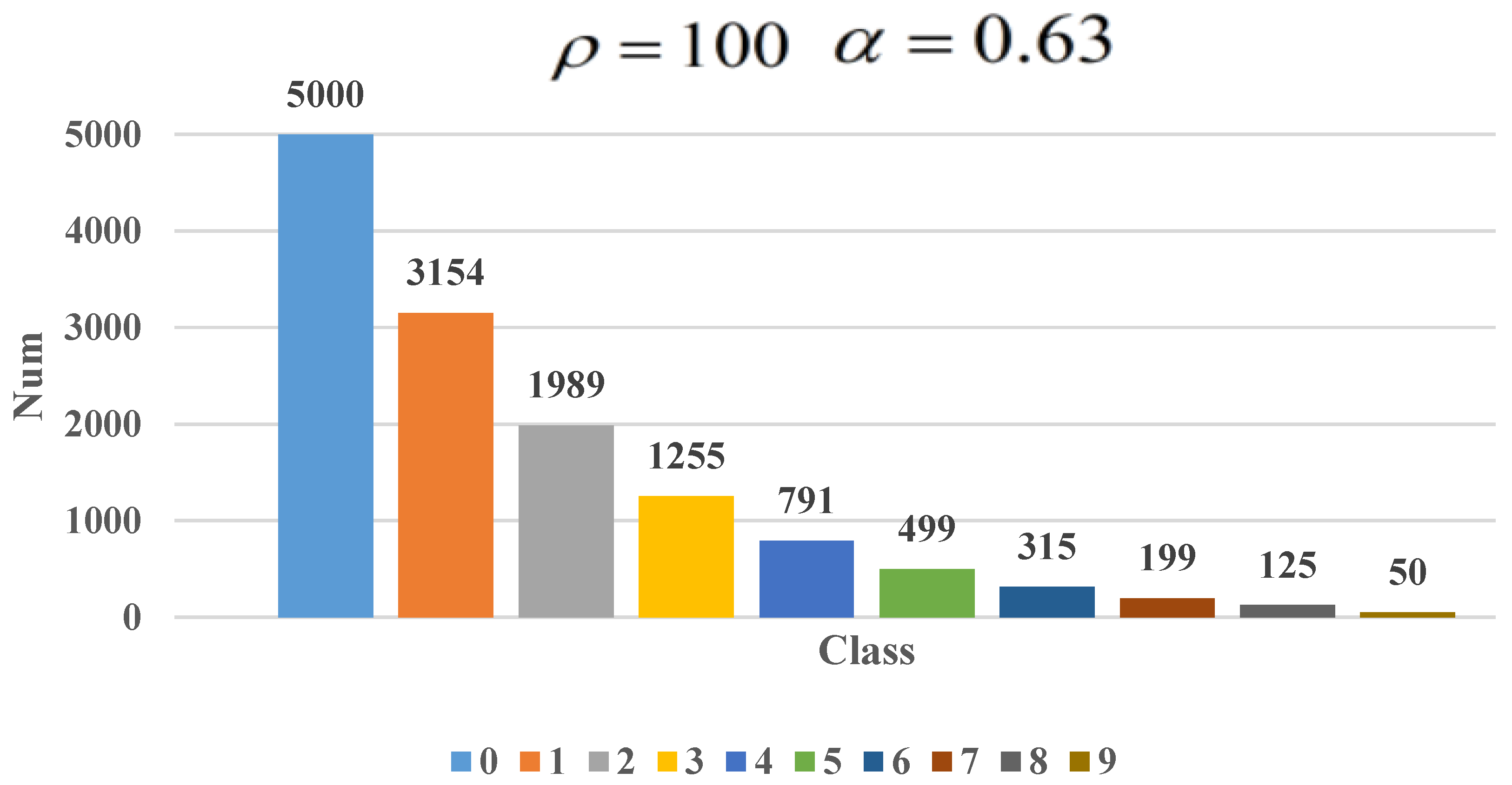
To create unbalanced datasets, this scheme uses an exponential function $n=n_i{\alpha }^i$ to process each data category in the dataset.

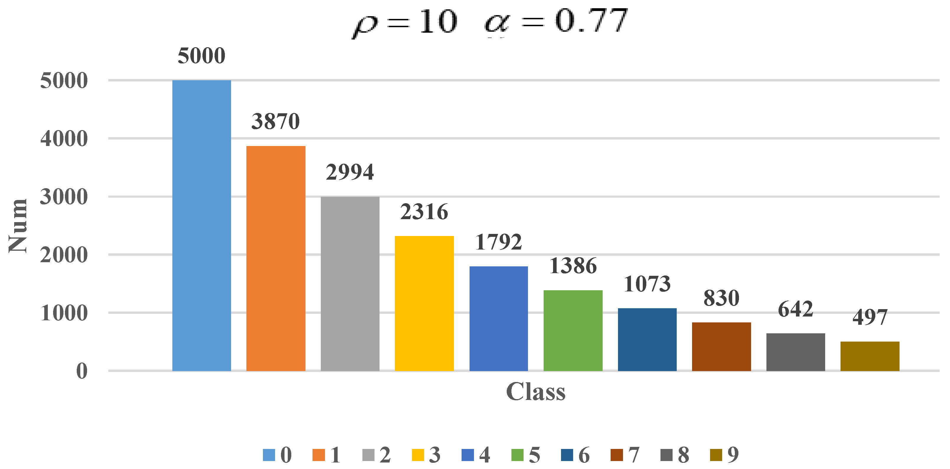
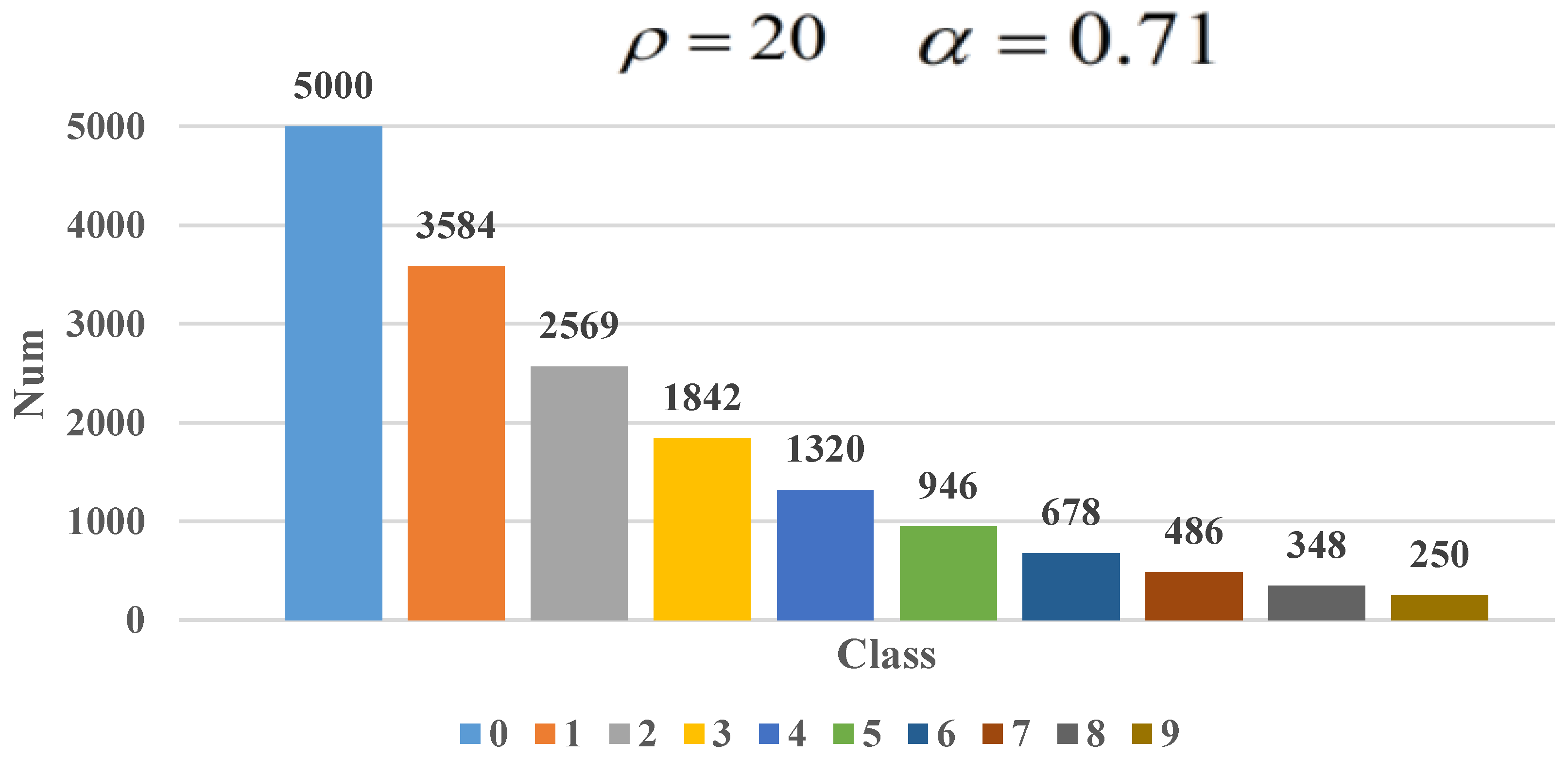
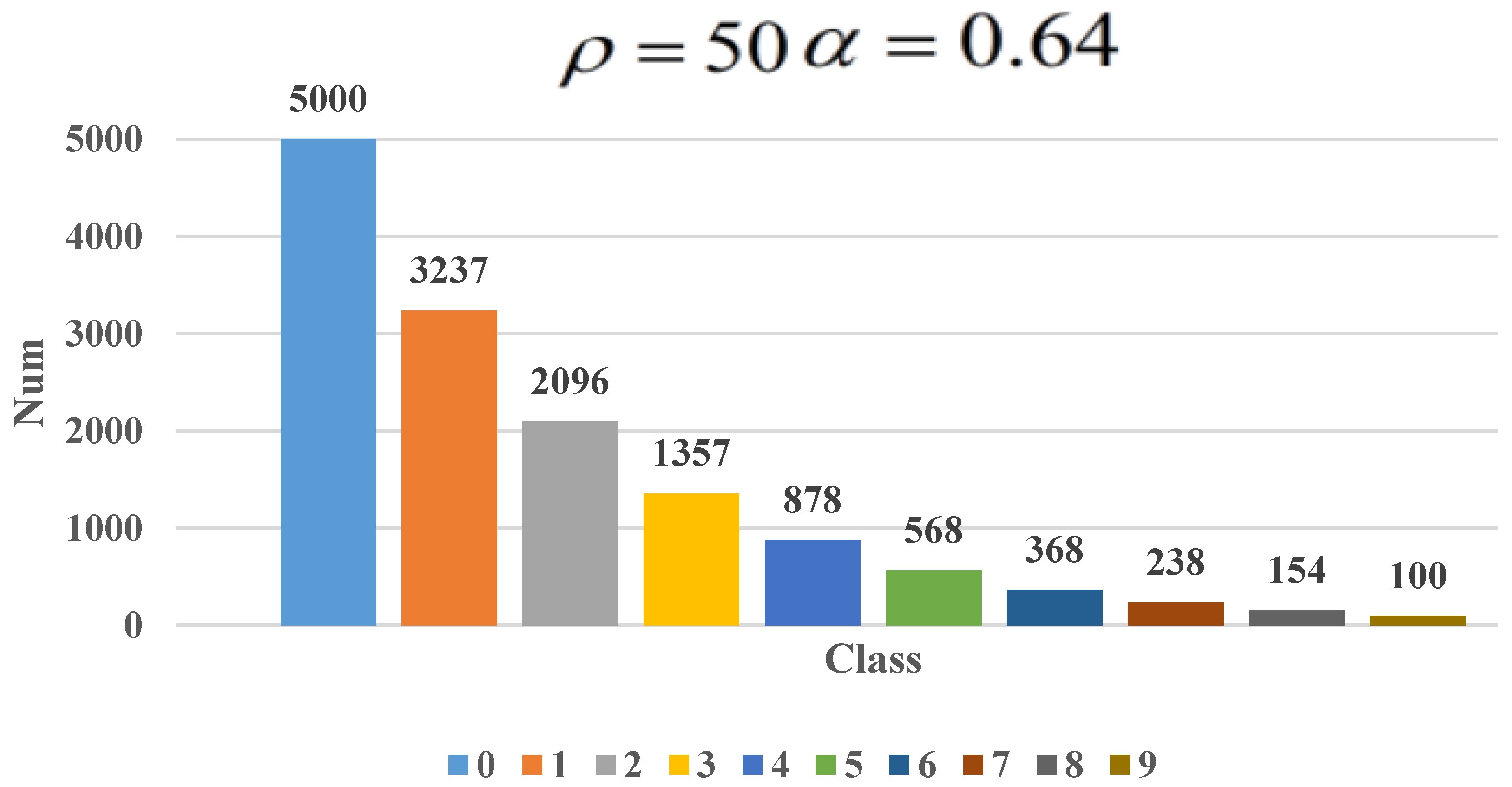
Determination of the hyperparameter $\alpha$: The value of $\alpha$ for each imbalance ratio (IR) is calculated by solving the equation $n_i{\alpha }^{m-1}=n_i/\mathrm{IR}$, where $n_i=5000$ is the original number of samples per class, and $m=10$ is the number of classes. This ensures that the smallest class (class 9) has $n_i/\mathrm{IR}$ samples. Rearranging gives $\alpha ={(1/\mathrm{IR})}^{1/(m-1)}$. Specifically, for IR = 10, $\alpha ={(1/10)}^{1/9}\approx 0.77$; for IR = 20, $\alpha ={(1/20)}^{1/9}\approx 0.71$; for IR = 50, $\alpha ={(1/50)}^{1/9}\approx 0.64$; for IR = 100, $\alpha ={(1/100)}^{1/9}\approx 0.63$.

$n_i$ is the number of categories i and $\alpha$ is a hyperparameter; according to different imbalance ratios, the value of parameter $\alpha$ is different. This exponential function processes the dataset into datasets with imbalance ratios of 10, 20, 50, and 100.

The data category distribution in each dataset and the value of it are shown in Figure 3, Figure 4, Figure 5 and Figure 6.

MNIST is a balanced dataset with 10 data categories, namely, 0, 1, 2, 3, 4, 5, 6, 7, 8, 9, and 5000 datapoints in each category. Figure 3 creates a dataset with an imbalance ratio of 10. According to the exponential function $n=n_i{\alpha }^i$, the value of $n_i$ is 5000, and the value of $\alpha$ is 0.77. Under different imbalance ratio conditions, the value of $\alpha$ is different, but the value of $n_i$ is still 5000.

Clarification on minority class designation: In our synthetic imbalance generation, classes are ordered such that class 0 is the majority (largest number of samples) and class 9 is the minority (smallest number of samples), with intermediate classes following an exponential decay in sample count. For each IR, the number of samples in class i is given by $n_i=5000\times {\alpha }^i$, where $\alpha$ is calculated as described in Section 4.4. This ensures a consistent and interpretable imbalance structure across experiments.

4.5. Data Oversampling Method

Imbalanced data will cause the training results of the model to tend to the majority class, thereby ignoring important data in the minority class. G-SMOTE is an effective method for balancing datasets. This paper improves this method to adapt it to the environment of multiple categories.

Complete G-MSMOTE parameter settings:

• Nearest neighbors: $k=5$ for all minority classes.
• Selection strategy: ${\alpha }_{sel}=S$ (entire dataset) for all imbalance ratios.
• Truncation factor: ${\alpha }_t=0$ (no truncation).
• Deformation factor: ${\alpha }_d=0.5$ (moderate deformation).
• Samples per minority class: Upsampled to match majority class count.
• Random seeds: 5 different seeds for reproducibility.
• Sensitivity analysis: Tested $k\in \{3,5,7\}$, ${\alpha }_d\in \{0.3,0.5,0.7\}$, ${\alpha }_{sel}\in \{S_n,S-S_n,S\}$.

Optimal configuration: The above parameters were selected based on grid search maximizing Macro-F1 score on the validation set for IR = 100. The configuration shows robustness across imbalance ratios.

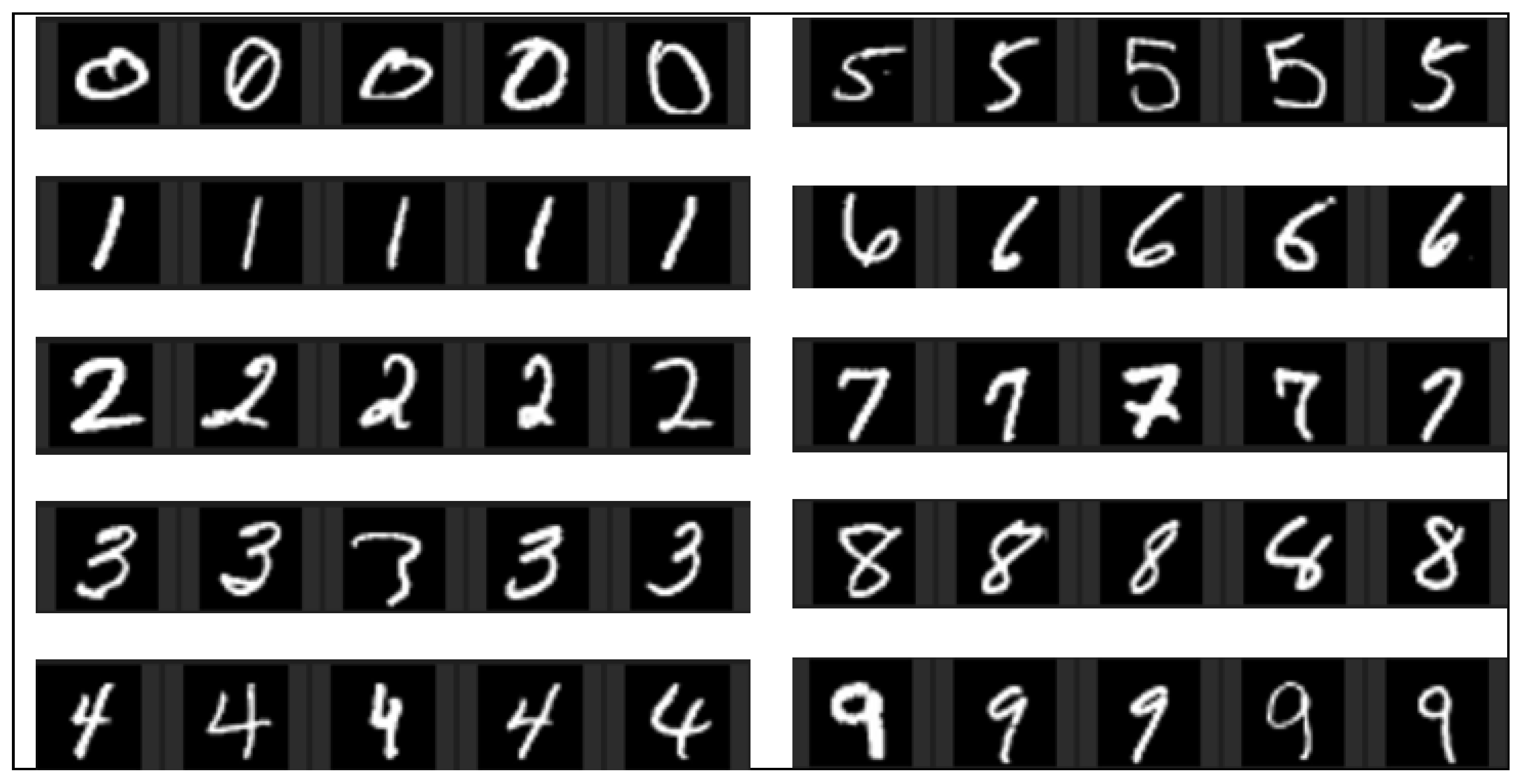
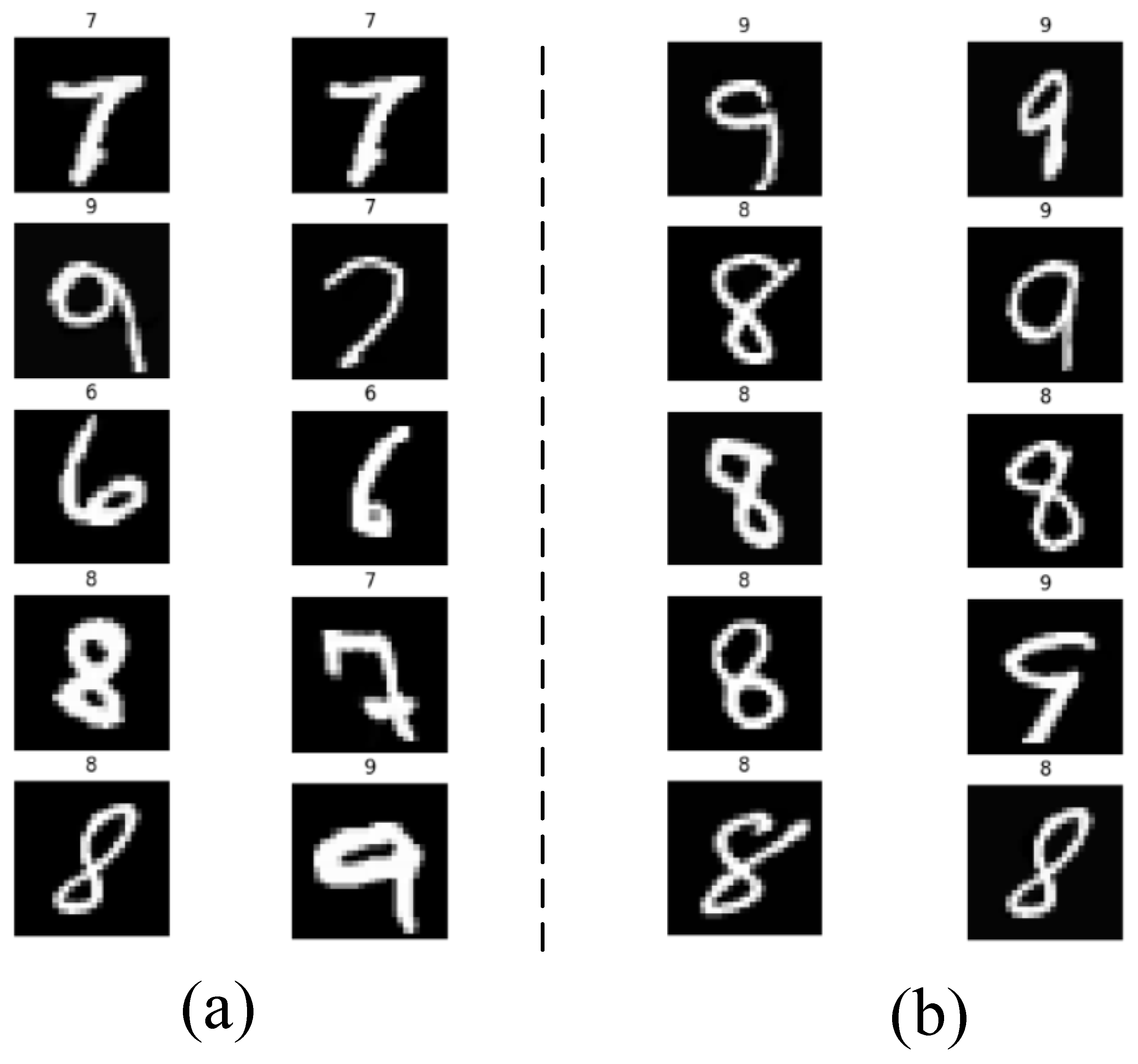
In the experiments of this paper, different minority classes were simulated for oversampling. Figure 7 shows the images in the original dataset, demonstrating the clarity and authenticity of each category of images. Figure 8a,b shows the synthesized images. The synthesized images are very clear compared to the original images. In Figure 8a, categories 6, 7, 8, and 9 are minority classes, and the G-MSMOTE algorithm generates a certain amount of data. In Figure 8b, the minority classes are categories 8 and 9. Through observation and comparison, it is found that the data generated by the G-MSMOTE algorithm can not only process multiple minority class data at the same time but also generate diverse samples, thereby increasing the amount of minority class data and balancing the distribution of data.

4.6. Training of Neural Networks

In neural network training, the core idea of this solution is to use plaintext datasets to train the neural network designed in this paper and use ciphertext for inference calculations in the inference phase. During the training of the neural network model, the loss will be amplified since the loss function uses a square operation. We use a gradient descent optimizer with 100 training rounds to prevent gradient explosion. The decay method gradually reduces the learning rate during the entire training process. The initial value of the learning rate is 0.01, set to 0.005 at the 30th epoch, and decayed to 0.0003 at the 60th epoch. The number of samples for each batch size is set to 100. Since memory is limited, a larger batch size will consume more video memory. We set the batch size to 100 to balance computational efficiency and memory limitations.

After training, to test the model’s performance in plain text, we use ACC, Macro-F1, and Micro-F1 values as indicators for verification. In the experiment, we trained on a balanced dataset and a dataset with an imbalance ratio of 10, 20, 50, and 100. To better demonstrate the oversampling effect of the G-MSMOTE scheme, we trained and verified on a dataset without executing the G-MSMOTE algorithm. The specific experimental results are shown in

Table 1. Results without oversampling (%). Values are mean ± standard deviation over 5 runs.

IR	0	10	20	50	100
ACC	94.37 ± 0.12	85.62 ± 0.25	76.56 ± 0.31	64.68 ± 0.42	55.93 ± 0.51
Macro-F1	94.39 ± 0.11	81.35 ± 0.28	68.53 ± 0.37	54.51 ± 0.45	43.20 ± 0.55
Micro-F1	94.37 ± 0.12	85.62 ± 0.25	76.56 ± 0.31	64.69 ± 0.42	55.94 ± 0.51

.

As shown in Table 1, when $IR=0$, that is, the dataset is balanced, our model achieves a prediction accuracy of 94.37%, Macro-F1 of 94.39%, and Micro-F1 of 94.37%. When the imbalance ratio becomes 10, the number of samples in the minority class decreases, leading to a decline in all metrics: ACC drops to 85.62%, Macro-F1 to 81.35%, and Micro-F1 to 85.62%. As the imbalance ratio increases further to 20, 50, and 100, the performance continues to degrade significantly. At $IR=100$, ACC is only 55.93%, Macro-F1 is 43.20%, and Micro-F1 is 55.94%. This demonstrates that class imbalance, especially the scarcity of minority samples, severely harms model performance.

Next, we apply the G-MSMOTE oversampling scheme to each imbalanced dataset (IR = 10, 20, 50, 100) to balance the class distribution, and then train and test the model. The results are shown in

Table 2. Results after G-MSMOTE oversampling (%). Values are mean ± standard deviation over 5 runs.

Metric	IR = 10	IR = 20	IR = 50	IR = 100
ACC	93.43 ± 0.15	84.68 ± 0.28	81.25 ± 0.35	72.81 ± 0.48
Macro-F1	93.45 ± 0.14	80.20 ± 0.31	76.90 ± 0.39	66.07 ± 0.51
Micro-F1	93.44 ± 0.15	84.69 ± 0.28	81.25 ± 0.35	72.81 ± 0.48

.

Comparing Table 1 and Table 2, we observe the following improvements after applying G-MSMOTE oversampling:

• IR = 10: Accuracy improves from 85.62% to 93.43%, a gain of 7.81 percentage points.
• IR = 20: Accuracy improves from 76.56% to 84.68%, a gain of 8.12 percentage points.
• IR = 50: Accuracy improves from 64.68% to 81.25%, a gain of 16.57 percentage points.
• IR = 100: Accuracy improves from 55.93% to 72.81%, a gain of 16.88 percentage points.

For imbalanced data, after applying the G-MSMOTE oversampling scheme proposed in this paper, the imbalance in the dataset is effectively alleviated, and the disparity in the number of samples across different categories is reduced. After oversampling, at an imbalance ratio of 10, the accuracy reaches 93.43%, which represents an improvement of 7.81 percentage points compared to before oversampling. At an imbalance ratio of 100, the accuracy is improved by 16.88 percentage points. After G-MSMOTE oversampling, the model’s ACC, Macro-F1, and Micro-F1 values on the dataset show significant improvement, though they still do not reach the performance level of a normally balanced dataset. The primary reason is that the generated data lacks diversity and exhibits a certain degree of similarity, leading to a weaker generalization ability of the model. Based on the above discussion, it can be concluded that, after implementing the G-MSMOTE scheme, the model’s performance is markedly better, demonstrating the effectiveness of our proposed scheme.

4.7. Ciphertext Data Prediction

To verify the performance of this scheme in the case of ciphertext, the plaintext is first encoded and encrypted on the user side, and the encryption result is transmitted to the cloud server. The cloud server completes the ciphertext data, makes a prediction based on the ciphertext, and returns the prediction result to the user. Only the user can decrypt the correct result. The prediction process involves encoding, data encryption, encrypted data prediction, decryption, and decoding operations.

Clarification on measured metrics and experimental setup: The following analysis reports the end-to-end wall-clock time for each stage (encoding, encryption, layer-wise computation) when processing a batch of 10,000 images as a single job. The reported times are total compute times measured on the server, encompassing both CPU and (where applicable) GPU operations. The ciphertext sizes are the actual persistent storage footprints of intermediate results. To address concerns about feasibility, we later decompose these times and provide a system-level analysis that separates compute, I/O, and estimated network transfer overheads, as shown in

Table 3. Complete FHE parameter specification and packing configuration.

Parameter	Symbol	Value	Rationale
Polynomial degree	n	4096	Provides 128-bit security under RLWE assumption
Ciphertext modulus	q	$q_1\times q_2\times q_3\times q_4\times q_5$	Product of five 60-bit primes for RNS decomposition
Plaintext modulus	t	$t_1\times t_2\times t_3\times t_4\times t_5$	Product of five 30-bit primes for CRT batching
Security level	$\lambda$	128 bits	Aligns with HE standard
Packing capacity	C	$n\times 5=20,480$ values	Each ciphertext encodes 5 images × 4096 slots
Images per ciphertext	m	5	Corresponds to five CRT channels ($t_i$)
Pixels per image	p	784	MNIST image size ($28\times 28$)
Ciphertexts for 10 k images	N	$\lceil 10,000\times 784/20,480\rceil =383$	Total ciphertexts needed for full batch
Ciphertexts for 10 k images	N	$10,000/5=2000$	Total ciphertexts needed for full batch (5 images per ciphertext)

.

Encoding. Before encrypting data, the plaintext data must be encoded to meet the requirements of the encryption algorithm while increasing the amount of information carried by each polynomial and reducing the computational space. In addition, the model parameters need to be encoded to meet the prediction of ciphertext data. Multiple files are formed during the encoding process. The description and size of each file are shown in

Table 4. Encoding files of data and model parameters.

File Name	Description	File Size
plain_layer0	The preprocessed data can be used as input for the encryption algorithm.	328,515.75 KB
dense1_kernel	Weights of the first fully connected layer after encoding.	3301.01 KB
dense1_bias	Bias of the first fully connected layer after encoding.	4.03 KB
dense2_kernel	Weights of the second fully connected layer after encoding.	39.19 KB
dense2_bias	Bias of the second fully connected layer after encoding.	0.52 KB
conv_kernel	The weights of the encoded convolutional layer.	5.01 KB
conv_bias	Bias of the encoded convolutional layer.	0.32 KB

.

Encoding and Encryption Details (revised for clarity): Encoding and Encryption Details (revised for clarity): We processed a total of 10,000 MNIST images for inference. Our packing scheme leverages the Chinese remainder theorem (CRT), as described in Section 3.3.1. With a polynomial degree of $n=4096$ and $k=5$ coprime moduli $t_i$, each ciphertext provides $n·k=\mathrm{20,480}$ independent integer slots.

For each pixel position (out of $28\times 28=784$ positions), we pack the corresponding pixel from five different images into the same polynomial slot using the five CRT residues. Concretely, the first 784 polynomial slots store the 784 pixel positions for five images; each slot contains five pixel values (one per image) encoded via the CRT decomposition. The remaining $4096-784=3312$ slots are padded with zeros.

Encoding and Encryption Details (revised for clarity): We processed a total of 10,000 MNIST images for inference. Our packing scheme leverages the Chinese remainder theorem (CRT), as described in Section 3.3.1. With a polynomial degree of $n=4096$ and $k=5$ coprime plaintext moduli $t_i$, we utilize the CRT to pack five images into a single ciphertext. Specifically, for each of the 4096 coefficient positions in the polynomial, we store the pixel values of five different images by encoding them into the five CRT residues. This means that, for each pixel position (out of $28\times 28=784$ positions), the five CRT residues at that coefficient position hold the corresponding pixel values from five distinct images. The remaining $4096-784=3312$ coefficient positions are padded with zeros.

Thus, a single ciphertext encodes ** exactly five complete images**, and one ciphertext operation simultaneously processes all five images. The total of 10,000 images therefore requires $\mathrm{10,000}/5=2000$ ciphertexts. The ‘plain_layer0’ file contains the CRT-encoded data for all 10,000 images prepared for encryption. The total encoding time of 26.34 s corresponds to an average of 0.002634 s per image.

Data encryption. After encoding the 10,000 images that need to be predicted, the plain_layer0 file is encrypted to form the ciphertext file enc_layer0, which is 3153.92 MB in size. The user uploads it to the cloud server for the next prediction operation. After the cloud server receives the ciphertext data, it uses the neural network to infer and predict it. The size of the output file of each layer of the network model during the prediction process is shown in

Table 5. Execution results of each network model layer during the prediction process.

Layers	Output File	Description	Execution Time	File Size
Convolution layer	enc_layer1	Encrypted data after the first convolutional layer and flattening.	20,277.67 s	3164.16 MB
Square activation layer	enc_layer2	Encrypted data after the second layer of the square activation function.	359.11 s	3169.52 MB
Full connectivity layer	enc_layer3	Encrypted data after the fully connected layer.	3249.26 s	444.0 MB
Square activation layer	enc_layer4	Encrypted data after the fourth layer of the square activation function.	106.41 s	375.0 MB
Output layer	enc_layer5	The ciphertext prediction data is finally output by the model.	77.35 s	44.4 MB

.

System-Level Performance Analysis: The runtime is dominated by the convolutional layer (≈20,278 s, 84% of total compute time) due to the high cost of homomorphic convolution, which requires rotating and summing large ciphertext vectors. The subsequent square activation and fully connected layers involve cheaper homomorphic additions and multiplications. The large intermediate ciphertext sizes (multi-GB) are inherent to FHE, as security requires large polynomial coefficients.

A realistic deployment scenario must account for three distinct cost factors:

• Compute Time: Reported in Table 5 (total: ≈24,070 s for 10 k images). This is the pure computational cost on the cloud server’s CPU.
• I/O Time: Writing and reading multi-GB ciphertexts between layers to persistent storage (e.g., SSD) adds overhead. We estimate this at approximately 15% of the compute time based on our disk benchmarks.
• Network Transfer Time: For a 3.15 GB input ciphertext (‘enc_layer0’) and a 44.4 MB output (‘enc_layer5’), transfer over a 1 Gbps network would add ≈27 s for upload and ≈0.36 s for download, which is negligible compared to compute time.

Per-Image Throughput Calculation: Our primary throughput metric is compute throughput. The total compute time of 24,070 s for 10,000 images yields an average of 2.41 s per image. This aligns with the capacity of our packing strategy: each homomorphic operation processes a batch of 20,480 pixel-mappings, and the 10,000 images utilize this capacity across multiple ciphertexts. This calculation is consistent with our packing strategy where each ciphertext encodes five images, resulting in 2000 ciphertexts for the full batch. The claim of g (or 0.4 images per second) is derived from this per-image compute time, excluding I/O and network latency.

Verifiable Throughput Analysis: As detailed in our packing strategy, the polynomial degree $n=4096$ and the use of five parallel CRT channels ($t_i$) allows each ciphertext operation to act on a vector of $4096\times 5=20,480$ encoded values. For 10,000 images of 784 pixels each, the total number of scalar values is 7.84 million. This requires approximately $7.84 M/\mathrm{20,480}\approx 383$ ciphertexts to represent the full batch. The total server-side compute time for this batch is 24,070 s (Table 5). Therefore, the amortized compute time per image is $\mathrm{24,070} s/\mathrm{10,000}=2.41$ s, and the system’s compute throughput is $\mathrm{10,000}/\mathrm{24,070}\approx 0.415$ images per second, or about 1494 images per hour. The previously stated 2.5 s/image (1440 images/h) was an approximation; this revised calculation provides a verifiable baseline. In a real-world setting, adding I/O overhead would reduce this throughput, emphasizing that computational cost remains the primary bottleneck for FHE-based inference.

Data decryption results. After the cloud server inference results in the enc_layer5 file is sent to the user, the user decrypts it to form a decrypted file. To verify the performance of the model parameters generated by unbalanced data training in ciphertext data, we verify it on the oversampled dataset and the non-oversampled dataset. The experimental results are shown in

Table 6. Ciphertext prediction accuracy with different oversampling methods (%). Values are mean over 5 runs.

IR	Accuracy (%)
	None	G-MSMOTE	ADASYN	Borderline	Safelevel	SMOTE
10	84.19	92.68	90.46	85.72	90.77	84.69
20	77.69	85.22	80.13	76.33	76.60	80.50
50	67.63	79.59	65.72	72.37	73.90	68.71
100	55.08	70.18	59.35	61.53	65.54	59.29

.

Table 6 Explanation: This table presents the prediction accuracy rates of the models trained with different oversampling methods on the encrypted data. “None” indicates the baseline method without oversampling. The results show that G-MSMOTE achieves the best performance across all imbalance ratios (IR).

According to Table 1, Table 2 and Table 6, the prediction results of the model in plaintext and ciphertext data differ by about 2%. This is because the plaintext data is rounded after the encoded data is multiplied by the precision constant K, which will lose some data. Because of the multiplication of the precision constant, the difference is within a controllable range. The accuracy of the prediction of ciphertext data in the balanced case reaches 93.44%. In Table 6, compared with multiple oversampling schemes, it can be seen that the prediction accuracy of the model trained using the dataset without oversampling is lower in the ciphertext data, and the imbalance ratio is 100. In this case, the accuracy is only 55.08%. After executing the G-MSMOTE scheme on the imbalanced dataset, the model’s accuracy in the ciphertext data reaches 70.18%. In the case of the same imbalance ratio of 100, the accuracy of SMOTE is only 59.29%. Although ADASYN and Borderline-SMOTE have improved the SMOTE method, the accuracy still needs to be significantly improved. The improved safe level-someone has an accuracy of 65.54%, but its accuracy is still lower than the solution we proposed. Our scheme also shows superiority when the imbalance ratio is 10, 20, and 50. Therefore, our solution not only ensures data security but also effectively improves model prediction accuracy in the case of imbalanced data.

5. Security Analysis and Discussion

5.1. Threat Model

We adopt the static semi-honest (honest-but-curious) adversarial model, consistent with prior work on FHE-based inference. In this model, the following are true:

• The adversary may corrupt either the client or the server (but not both), and corruption occurs at protocol initiation.
• Corrupted parties follow the protocol specification exactly but may attempt to learn additional information from their view (inputs, random coins, received messages).
• We do not consider active attacks (e.g., tampering, dropping messages) or side-channel attacks (timing, power).

Allowed Leakage. We explicitly state what information is considered non-sensitive and thus may be revealed (leaked):

• Neural network architecture: Number of layers, layer types (convolutional, fully connected), activation functions.
• FHE parameters: Polynomial degree n, ciphertext modulus q, plaintext modulus t.
• Circuit metadata: Number of multiplications, ciphertext dimensions, and sizes.
• Execution metadata: The fact that computation occurs, but not timing information.

Our security goal is to protect the following:

• Client input privacy: The server learns nothing about the client’s input data beyond the classification result.
• Model parameter confidentiality: The client learns nothing about the server’s model weights beyond the classification result.

5.2. Protocol Description

Our secure classification protocol $\Pi$ is executed between a client $\mathcal{C}$ (data owner) and a server $\mathcal{S}$ (model owner). Let $\mathrm{FHE}=(\mathrm{KeyGen}, \mathrm{Enc}, \mathrm{Dec}, \mathrm{Eval})$ be a CPA-secure fully homomorphic encryption scheme.

Initialization Phase:

• $\mathcal{C}$ runs $(pk,sk)\leftarrow \mathrm{FHE}.\mathrm{KeyGen}\left(1^{\lambda }\right)$ and sends $pk$ to $\mathcal{S}$.
• $\mathcal{S}$ trains a neural network f, encodes weights as described in Section 3.3, and keeps them secret.

Classification Phase (per query):

• Input Encryption: $\mathcal{C}$ encodes input x using CRT (Section 3.3.2), computes $c{t}_x\leftarrow {\mathrm{FHE}.\mathrm{Enc}}_{pk}\left(x\right)$, and sends $c{t}_x$ to $\mathcal{S}$.
• Homomorphic Evaluation: $\mathcal{S}$ computes $c{t}_y\leftarrow {\mathrm{FHE}.\mathrm{Eval}}_{pk}(f,c{t}_x)$ layer by layer, exactly as in Section 3.2.
• Result Return: $\mathcal{S}$ sends $c{t}_y$ to $\mathcal{C}$.
• Decryption: $\mathcal{C}$ computes $y\leftarrow {\mathrm{FHE}.\mathrm{Dec}}_{sk}\left(c{t}_y\right)$ and decodes to obtain the classification result.

5.3. Security Analysis

Definition 1. 

Ideal Functionality ${\mathcal{F}}_{\mathit{Classify}}$ The ideal functionality for secure classification behaves as follows:

1. 

Upon receiving x from $\mathcal{C}$, send $\mathsf{classify}$ to $\mathcal{S}$.

2. 

Upon receiving f from $\mathcal{S}$, compute $y=f\left(x\right)$.

3. 

Send y to $\mathcal{C}$ and nothing to $\mathcal{S}$.

Theorem 1 

(Security against semi-honest adversaries). Let $\mathsf{FHE}$ be a CPA-secure fully homomorphic encryption scheme. Then, protocol $\Pi$ preserves the confidentiality of the client’s input and the server’s model parameters in the semi-honest model, with at most the leakage $\mathcal{L}$ defined in Section 5.1.

Argument. We consider the two corruption cases separately.

• Case 1: Corrupt Server ${\mathcal{S}}^{*}$. The server’s view consists of the public key $pk$ and the ciphertext $c{t}_x=\mathsf{FHE}.{\mathsf{Enc}}_{pk}\left(x\right)$. By the CPA-security of the FHE scheme, $c{t}_x$ is computationally indistinguishable from an encryption of any other message of the same length. Consequently, ${\mathcal{S}}^{*}$ learns nothing about the client’s private input x beyond what is implied by the public parameters and the leakage $\mathcal{L}$ (e.g., the size and format of x). The subsequent homomorphic evaluation ${\mathsf{Eval}}_{pk}(f,c{t}_x)$ is performed entirely on encrypted data and does not provide any additional leakage about x.
• Case 2: Corrupt Client ${\mathcal{C}}^{*}$. The client’s view includes its own input x, the secret key $sk$, the public key $pk$, and the result ciphertext $c{t}_y={\mathsf{Eval}}_{pk}(f,c{t}_x)$. Upon decryption, ${\mathcal{C}}^{*}$ learns only the output $y=f\left(x\right)$. The CPA-security of FHE guarantees that the ciphertext $c{t}_y$ (and the evaluation process that produced it) reveals no information about the server’s private model f beyond the output y and the declared leakage $\mathcal{L}$ (e.g., the network architecture and FHE parameters needed to perform the computation).
• In both cases, the protocol does not reveal any information beyond the explicitly allowed leakage $\mathcal{L}$ and the functional output y. Therefore, $\Pi$ achieves the security goals stated in Section 5.1 under the semi-honest adversarial model.

5.4. Practical Security and Parameter Instantiation

Mapping to SEAL/BFV Instantiation. Our implementation uses Microsoft SEAL’s BFV scheme, whose security relies on the Ring-Learning With Errors (RLWE) assumption. We instantiate parameters following the Homomorphic Encryption Security Standard:

• Polynomial degree: $n=4096$ (ring dimension).
• Ciphertext modulus: $q={\prod }_{i=1}^5{q}_i$, where each $q_i\approx 2^{60}$ is a 60-bit prime.
• Plaintext modulus: $t={\prod }_{i=1}^5{t}_i$, where each $t_i$ is a 30-bit prime.
• Error distribution: Discrete Gaussian with standard deviation $\sigma =3.19$.

These parameters achieve 128-bit security under the RLWE assumption, matching the “HEstd_128” level in the standard.

Security Claims Clarification. We emphasize that our contribution is a system integration of geometric oversampling with standard FHE-based inference. The cryptographic security of our scheme reduces to the well-established CPA-security of the BFV scheme in the semi-honest model, with the explicitly defined leakage profile.

Limitations and Future Work. Our analysis does not address the following:

• Active adversaries or malicious behavior;
• Side-channel attacks (timing, memory access patterns);
• Circuit privacy (hiding the function f evaluated).

Extensions to stronger security models (e.g., malicious security) would require additional cryptographic techniques beyond standard FHE.

6. Conclusions

In this paper, we analyze the privacy security and data imbalance issues in data classification tasks in a big data environment and summarize the consequences of these issues. Based on these issues, we propose an unbalanced data classification scheme based on CryptoNets. Through CRT technology and homomorphic encryption, we ensure that data is available and invisible so that cloud servers can perform reasoning and prediction tasks on ciphertext data, solving the privacy security issues in data classification tasks. Data imbalance will cause the network model to tend to the majority class and ignore important minority-class data. By oversampling multiple minority classes to generate diverse and low-noise data, the data imbalance problem is alleviated. Finally, experiments were conducted on the MNIST dataset under different imbalances. The experimental results show that the model performs well in unbalanced data and effectively saves polynomial space. The encryption scheme is a difficult problem based on Ring Learning With Errors (RLWE). Under current technical means, it is difficult for attackers to successfully attack, and the scheme has a certain degree of security.

In the data encoding part, the encoded file size is 328,515.75 KB; after encrypting the data, it becomes 3153.92 MB. Our solution requires a lot of memory resources and is difficult to apply in edge devices with scarce resources. At the same time, without considering network latency, the actual time for encoding, encrypting, and predicting an image is about 2.5 s. Although the calculation time is fast, the file is a 28*28 image. If the image is larger, the calculation time will double. In actual medical applications, the size of an image is generally 512*512, which will take a long time to calculate. Therefore, in future research, we will study solutions with faster computing efficiency and smaller resources, reduce the time required for data inference and prediction, expand the applicable scenarios of the solution, and protect data privacy and security.

Limitations and Future Work: While our study demonstrates the feasibility of combining geometric oversampling with privacy-preserving inference, we acknowledge several limitations. First, our experiments use MNIST with synthetically generated imbalance, which serves as a controlled benchmark but does not fully capture the complexity of real-world imbalanced data (e.g., overlapping minority classes, label noise, or multi-modal distributions). Second, the computational overhead of fully homomorphic encryption currently restricts application to larger, more complex datasets typical in medical imaging.

To address these limitations, future work will focus on (1) evaluating our framework on inherently imbalanced medical datasets (e.g., skin lesion classification, retinal scans) with realistic class overlap and noise; (2) extending the per-class evaluation to include detailed precision, recall, and F1-score breakdowns for each minority class; and (3) optimizing the cryptographic parameters and neural architecture to reduce inference time while maintaining security guarantees. These steps are essential for translating our proof-of-concept into practical clinical decision support systems.