Algebraic Properties of Generalized Trigonometric Function Transforms

Abstract

The generalized trigonometric functions called Ateb-functions are considered. On this basis, a generalization of the Fourier transform is constructed and called the Ateb-transform. From the operator theory point of view, the Ateb-transform is considered as a formalism of the convolution algebra in which multiplication is defined by means of hypergroups of the generalized shift operator. In this formal approach, the algebraic structure is presented, and its properties are developed. The eigenvalue problem for the differential equation of nonlinear oscillation is investigated. Some properties are illustrated numerically. The application of this approach for modeling vibration motion is considered.

1. Introduction

Periodic and hyperbolic Ateb-functions were defined in the remarkable work in [1]. A few years later, their functional properties were generalized and investigated in Ref. [2]. The introduced periodic Ateb-functions are used to construct solutions of nonlinear differential equations of oscillatory systems. In these papers, the solutions provided in Ateb-function form were used to study stationary oscillations in essentially nonlinear systems that interact with an energy source. Later, the theory of Ateb-functions was further developed in Ref. [3]. In this paper, the orthonormality of periodic Ateb-functions was proved. This made it possible to study the single-frequency nonlinear oscillations of one-dimensional bodies in resonant and non-resonant cases. Longitudinal and torsional oscillations of nonlinear elastic shafts and rods fixed in various ways were studied. The theory of Ateb-functions is based on the asymptotic method of nonlinear mechanics [4]. This work shows that the application of Ateb-functions can be extended to all areas where ordinary trigonometric functions are used, thereby increasing the research tools.

It is known that modern telecommunication systems are based on the formal apparatus of the theory of harmonic functions [5], which can be represented as a complex exponential. Why were these particular functions chosen? Firstly, it is the naturalness of generating such oscillatory processes, and, secondly, invariant transformations leave the harmonic signals unchanged, while such transformations only weaken them (i.e., reduce the amplitude) and delay them in time: $F\left[a{e}^{ix}\right]=ka{e}^{i(x-\varphi )}$, where F is the system operator, a is the amplitude, $\varphi$ is the delay (phase), and k is the coefficient. These facts make it possible to use operator theory, in particular Laplace or Fourier transforms, for processing signals.

The formal mathematical apparatus of Fourier analysis provides a transition from time functions in time space to frequency functions, i.e., Fourier values of time functions in the frequency domain. However, representation of signals by sinusoidal functions is only one of many possible ways. It is known from functional analysis that any complete orthonormal system of functions can be used for decomposition as a basis, which is analogous to Fourier decomposition. Among them, decompositions by Bessel functions were demonstrated in Refs. [6,7]. For such decompositions, the modulation methods exist that correspond to amplitude, frequency, and phase modulation of the harmonics.

The exact action–angle variables for a class of purely nonlinear oscillators, enabling their dynamics to be represented in a canonical Hamiltonian form despite the absence of linear stiffness, were derived in Ref. [8]. This formulation provides a powerful analytical framework for determining frequency–amplitude relations, phase trajectories, and energy-dependent properties of strongly nonlinear oscillatory systems. The application of Ateb and generalized trigonometric functions for solving nonlinear oscillator problems was explored in Ref. [9], demonstrating how these functions can express analytical solutions for strongly nonlinear dynamics and showing their effectiveness compared to classical techniques.

Extensions to models with time-variable nonlinearity were studied in Ref. [10], opening analytical pathways for describing mechanical aging phenomena in engineered composites, again using generalized functional frameworks that extend classical constant-nonlinearity models. An approximate analytic expression for the vibration frequency of strong nonlinear polynomial oscillators was proposed in Ref. [11], whereby the nonlinear frequency is expressed as a function of amplitude and nonlinearity order with high accuracy across a wide parameter range. This method provides a useful tool for practitioners dealing with non-integrable nonlinear systems.

Mixed Fourier series based on smooth closed-form functions with compact support were introduced in Ref. [12], providing an alternative orthogonal basis for signal representation beyond classical sinusoidal functions. Their approach demonstrates improved localization and reduced Gibbs phenomena, making it particularly effective for representing non-stationary and sharply varying signals in modern signal processing applications. Beyond the Ateb-function-specific literature, there is a broader trend toward developing robust analytic methods for nonlinear dynamical systems. For instance, in Ref. [13], the non-perturbative approach was applied to obtain accurate periodic solutions of strongly nonlinear oscillators without relying on small parameter assumptions, illustrating the power of modern semi-analytic techniques in nonlinear analysis. Similarly, complex nonlinear behaviors (including chaos and stability) in novel micro-electromechanical oscillators were investigated, underscoring the diversity of modern nonlinear oscillator models and the necessity of advanced analytical methods for their study [14].

A further development of the idea of orthogonal representation (decomposition) is to use T-invariant processes for this purpose, where T is the shift operator [15]. Ateb-functions are orthogonal functions, so it is possible to use the algebraic interpretation of the idea of T-classes with respect to Ateb-functions as elements of the basis of signal spaces for special communication tasks.

This investigation extends the ideas presented in works [15,16]. The main contributions are

• The introduction of Ateb-transforms is presented, and their properties are investigated. It is shown that the set of these operators with addition and multiplication operations creates the algebra structure under the domain $L^2\left(R\right)$.
• The eigenfunction problem is discussed. It is shown that Ateb-functions are the eigenfunctions for the nonlinear oscillatory differential equation with initial values.
• Numerical examples are presented for illustration.

The article is organized as follows. The Introduction defines the problem and highlights the main results. Section 2 provides a brief review of the literature. Section 3 presents the main results related to the Ateb- transform, where some theorems are proved using the considered properties. Section 4 introduces calculation algorithms and numerical results that illustrate the theoretical concepts. The conclusion summarizes the study. The main definitions and formulas for the periodic Ateb-functions are provided in Appendix A.

2. Related Works

The concept of a truly nonlinear oscillator with position-dependent mass was explored in Ref. [17]. The mathematical model of its motion is based on solving the Cauchy problem for a significantly nonlinear second-order differential equation with zero initial conditions. The analytical solution of this model is presented using Ateb-cosine, and the amplitude of the vibrations and their frequencies are determined. Additionally, the period of vibration was calculated to assist in modeling and optimizing the motion of a truly nonlinear oscillator [17]. Article [18] presented an analytical solution for damped nonlinear oscillators of both integer and non-integer orders regardless of their complexity. It identifies the ratio of coefficients necessary to ensure the existence of the solution. The method for finding exact solutions relies on the application of Ateb-function theory. Practical examples are provided for various levels of nonlinearity: an almost linear oscillator, a Duffing oscillator, and an oscillator with strong nonlinearity. The models of the oscillatory motion based on Ateb-functions demonstrate their high solution accuracy [18].

Article [19] deals with modeling and optimization of a Liénard oscillator with the following properties: quadratic damping, nonlinear deflection, and constant excitation. In special cases, the analytical solution of this type of oscillator is given based on Ateb-function theory. In the process industry, the obtained research results for the Liénard equation are used to optimize the oscillator properties [19]. Paper [20] proposed a new method for examining the periodic solutions of certain physically highly nonlinear oscillators. In Ref. [21], an algorithm for calculating the hyperbolic Ateb-functions was discussed, a generalization of the Fourier transform based on Ateb-functions was constructed, and the general properties of this transform were investigated. In contrast to [21], the presented research focuses on the algebraic properties of Ateb-transforms. A q-calculus generalization of Ateb-functions was suggested in Ref. [21].

The applications of the shift operator to signal processing were presented in the literature. Paper [22] investigated how time-shift operators behave in a wide class of functional spaces that generalize classical $L^p$ spaces. It established rigorous criteria for when sequences of time shifts converge weakly, which is fundamental for understanding stability and averaging of translated signals. In Ref. [23], the authors analyzed how fast repeated time shifts converge to their long-term average in ergodic systems. Their results provide quantitative bounds on convergence rates, which is crucial for signal averaging and time-invariant data analysis.

A brief analysis of the recent publications indicates a general trend in the field of vibration modeling, which is the combination of improved mathematical analytical methods with modern numerical strategies and advanced signal processing techniques. Thus, the theory of Ateb-functions is actively developing as an analytical tool for the study of strongly nonlinear oscillatory systems.

3. Ateb-Transform Operators and Their Properties

In this chapter, we extend the idea of the Fourier transform to a transform based on Ateb-functions, called the Ateb-transform. We also use the generalization of a shift operator for Ateb-functions.

3.1. Definition of Ateb-Transform

Let $x\left(t\right)\in L^2\left(R\right)$ be a real function. We construct Ateb-transform in the form

$$X(m,n,\omega )=A(m,n,\omega )-iB(n,m,\omega ),$$

(1)

where

$$A(m,n,\omega )={\int }_{-\infty }^{\infty }x\left(t\right)·c{a}^m(m,n,\omega t)dt,$$

(2)

$$B(n,m,\omega )={\int }_{-\infty }^{\infty }x\left(t\right)·s{a}^n(n,m,\omega t)dt,$$

(3)

$ca(m,n,\omega )$ is Ateb-cosine and $sa(m,n,\omega )$ is Ateb-sine. Taking into account expression (A8), we obtain the formula for the inverse transform

$$x(m,n,t)={\displaystyle \frac{1}{2\Pi (m,n)}}{\int }_{-\infty }^{\infty }\{A(m,n,\omega )ca(m,n,\omega t)+iB(n,m,\omega )sa(n,m,\omega t)\}d\omega ,$$

(4)

where $\Pi (m,n)$ is a half-period of Ateb-functions. In the case $n=1$ and $m=1$, the introduced Equations (1)–(3) for Ateb-transform become well-known orthogonal Fourier transform formulas, and Equation (4) becomes the inverse Fourier transform.

3.2. Generalized Shift Operator

Let $f\left(x\right)\in L^2\left(R\right)$. In Ref. [15], the generalized shift operator was used for Ateb-functions for the first time. A classical shift operator $U^s$ is defined by formula

$$U^{s}f\left(t\right)=f(t+s).$$

We can define a set of shift operators with all real numbers $\{U^s,s\in R\}$.

The generalization $T_s$ of the shift operator $U^s$ is defined in the form

$$T_{s}f\left(t\right)={\displaystyle \frac{1}{2}}[U^{s}f\left(t\right)+\overline{U^s}f\left(t\right)+{\int }_{t-s}^{t+s}f\left(\tau \right)d{\mu }_{\tau ,\sigma }\left(u\right)],$$

(5)

where $\overline{U^s}$ is a complex conjugation for $U^s$, and ${\mu }_{\tau ,\sigma }\left(u\right)$ is some measure.

Definition 1.

Hypergroup superposition.

For every two generalized shift operators $S_{\tau }$ and $S_{\sigma }$, there exists a measure ${\mu }_{\tau ,\sigma }$ that satisfies the next equation

$$S_{\tau }\ast S_{\sigma }=\int S_{u}d{\mu }_{\tau ,\sigma }\left(u\right).$$

(6)

Superposition of two generalized shift operators is not directly a generalized shift operator but integral shift superposition that is inherent for the hypergroup.

Definition 2.

Convolution.

For $f\left(x\right)\in L^2\left(R\right)$ and $g\left(x\right)\in L^2\left(R\right)$, define a convolution operator by the next expression

$$(f\circ g)\left(t\right)={\int }_0^{t}f\left(t\right){\overline{T}}_{s}g\left(t\right)d\mu (s,t).$$

(7)

Thus, in this subsection, we define the generalized shift operator and its properties.

3.3. Algebra for Ateb-Transform Operators

Consider function $f\left(x\right)\in L_2\left(R\right)$ that is periodic with respect to an arbitrary variable x on the interval $[-\Pi (m,n),\Pi (m,n\left)\right]$ (see (A3)). Assume that function $f\left(x\right)$ is continuous and has no extrema on the given interval. Then, Fourier series for such function converges on the entire interval $[-\Pi (m,n),\Pi (m,n\left)\right]$, and the series based on Ateb-functions

$$f\left(\omega \right)={\displaystyle \frac{a_0}{2}}+\sum _{p=1}^{\infty }[a_{p}ca(m,n,{\displaystyle \frac{p\pi \omega }{\Pi (m,n)}})+b_{p}sa(n,m,{\displaystyle \frac{p\pi \omega }{\Pi (m,n)}})],$$

(8)

where

$$a_p={\displaystyle \frac{1}{\Pi (m,n)}}{\int }_{-\infty }^{+\infty }f\left(q\right)ca(m,n,p\Pi (m,n)q)dq,$$

$$b_p={\displaystyle \frac{1}{\Pi (m,n)}}{\int }_{-\infty }^{+\infty }f\left(q\right)sa(n,m,p\Pi (m,n)q)dq,$$

will also be convergent. On this basis, we can construct the algebra of Ateb-transform operators in the form $A=(S,W)$, where S is the set of X operators and W is the signature of algebra $A.$ The set of operations W contains ‘addition’ and ‘multiplication’. The addition operation is the usual addition of functions (correctness follows from the additivity of addition for integrals), and multiplication is defined by convolution (7). The algebra A satisfies the additivity condition.

Theorem 1.

Additivity Property.

Let functions $f\left(x\right)\in L^2\left(R\right)$ and $g\left(x\right)\in L^2\left(R\right)$ be continuous and have no extrema on the given interval. Then, for every nonzero real number α and β, we have

$$X(\alpha f+\beta g)=\alpha Xf+\beta Xg.$$

(9)

Proof. 

From the introduced Equations (1)–(3) and the additivity of the integral for Ateb-transform, we have

$$\begin{gathered} X(\alpha f+\beta g)= \\ ={\int }_{-\infty }^{\infty }(\alpha f+\beta g)·c{a}^m(m,n,\omega t)dt-i{\int }_{-\infty }^{\infty }(\alpha f+\beta g)·s{a}^n(n,m,\omega t)dt= \\ =\alpha {\int }_{-\infty }^{\infty }f·c{a}^m(m,n,\omega t)dt-i\alpha {\int }_{-\infty }^{\infty }f·s{a}^n(n,m,\omega t)dt+ \\ +\beta {\int }_{-\infty }^{\infty }g·c{a}^m(m,n,\omega t)dt-i\beta {\int }_{-\infty }^{\infty }g·s{a}^n(n,m,\omega t)dt=\alpha Xf+\beta Xg. \end{gathered}$$

The additivity is proven.    □

Theorem 2.

Convolution Theorem

Ateb-transform operator for the multiplication of two functions in the time domain equals the multiplication of Ateb-transform operator results in the frequency domain

$$X\left(fg\right)=X\left(f\right)\circ X\left(g\right).$$

(10)

Proof. 

The multiplicity follows directly from the convolution definition (7) and the integral properties.    □

Theorem 3.

Associativity Property

For every three functions $f,g$, and h from $L^2\left(R\right)$, we have the next associativity property

$$X\left(\right(fg\left)h\right)=\left(X\right(f)\circ X(g\left)\right)\circ X\left(h\right)=X\left(f\right)\circ \left(X\right(g)\circ X(h\left)\right)=X\left(f\right(gh\left)\right).$$

(11)

Proof. 

The associativity directly results from the hypergroup superposition definition (6). The property is proven.    □

Theorem 4.

The existence of the identity element for multiplication.

Dirac δ-function is an identity element for multiplication in A algebra

$$X\circ \delta =X.$$

(12)

Proof. 

It follows directly from Dirac $\delta$-function definition. We have the next equation $X\left(t\right)=\int \delta (t-s)X\left(s\right)ds.$ The identity operator on $L^2$ admits the distributional kernel

$$K_I(x,y)=\delta (x-y),$$

meaning that, for all f,

$$f\left(x\right)={\int }_{-\infty }^{+\infty }\delta (x-y)f\left(y\right)dy,$$

and the identity extends to all functions of $L^2$. The property is proven.    □

So, in this subchapter, we proved the algebraic properties of Ateb-transforms. Thus, the set of Ateb-transforms creates an algebra structure under the space of the real functions $L^2\left(R\right)$ with addition as a simple addition of functions and multiplication as their convolution.

3.4. Eigenfunctions for Nonlinear Oscillatory Equation

The periodic Ateb-functions $ca(m,n,t)$ and $sa(n,m,t)$ are particular solutions of the nonlinear oscillatory equation

$${\displaystyle \frac{d}{dt}}\left(\right|x^{\prime }{\left(t\right)|}^{m-1}{x}^{\prime }{\left(t\right))+|x\left(t\right)|}^{n-1}x\left(t\right)=0,$$

(13)

where $m>0$ and $n>0$. Equation (13) is the generalization of well-known linear differential equation of harmonic oscillations in the case $n=1,m=1$ in the form

$$x^{″}\left(t\right)+x\left(t\right)=0.$$

(14)

Let us introduce the differential operator $L_m$ in the form

$$L_m\left[x\left(t\right)\right]=-{\displaystyle \frac{d}{dt}}\left(\right|x^{\prime }\left(t\right){|}^{m-1}{x}^{\prime }\left(t\right)),$$

(15)

and consider equation

$$L_m\left[x\left(t\right)\right]=\lambda {\left|x\left(t\right)\right|}^{n-1}x\left(t\right),$$

(16)

for eigenvalues $\lambda (\lambda >0)$ of nonlinear differential Equation (13).

When we add the initial condition $x\left(0\right)=0$ and $x^{\prime }\left(0\right)=1$ to Equation (16), we obtain the eigenfunction in the form of Ateb-sine: $x\left(t\right)=sa(n,m,t)$, and, if we add the initial condition $x\left(0\right)=1$ and $x^{\prime }\left(0\right)=0$, we get the Ateb-cosine: $x\left(t\right)=ca(m,n,t)$ eigenfunction. Thus, Ateb-functions are the eigenfunctions of Equation (16) with the same eigenvalue ${\lambda }_0.$ By the analogy with the classic oscillation, we can consider ${\lambda }_0$ as an eigenvalue for the first (main) Ateb-harmonic. 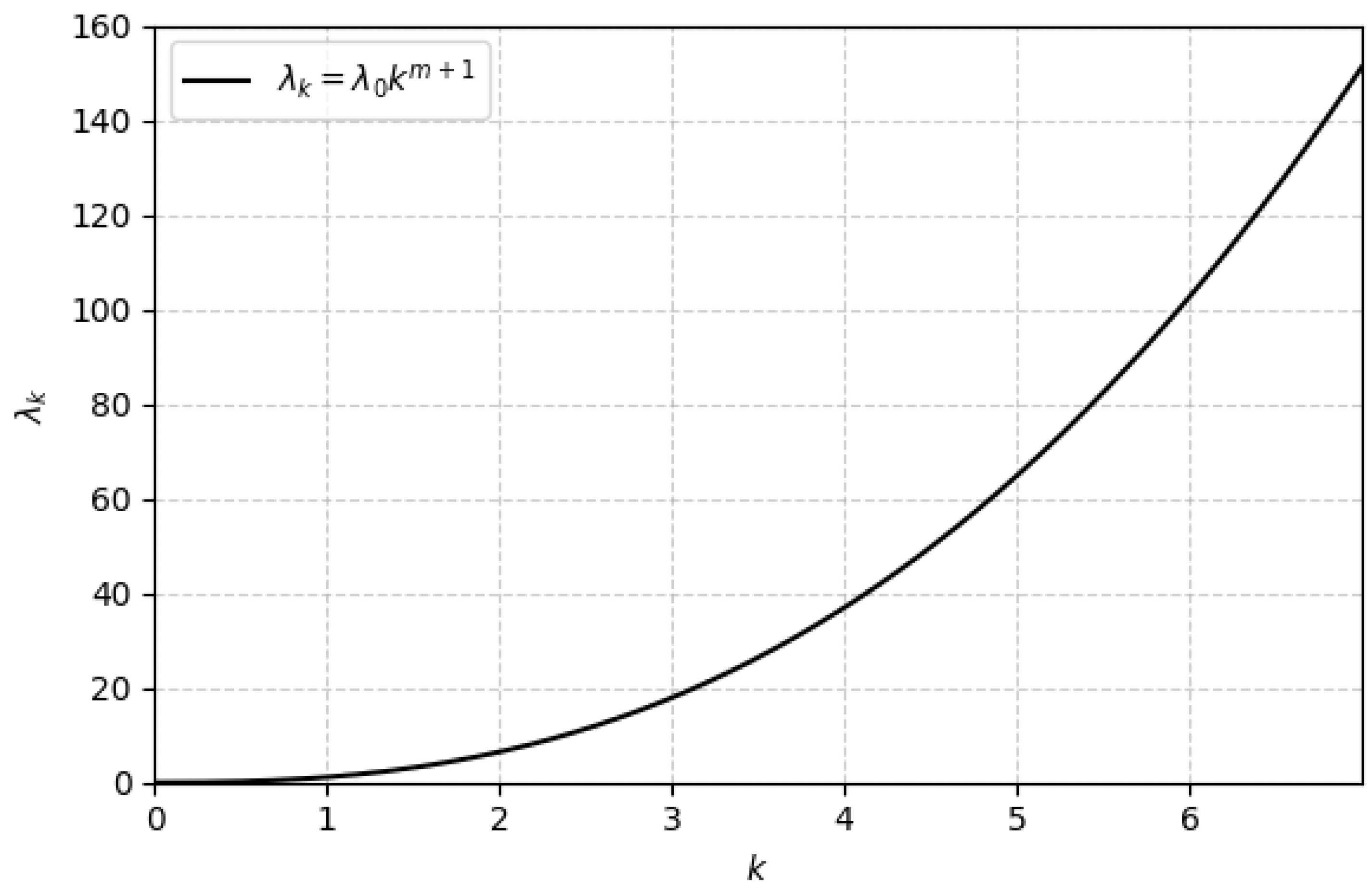For any integer $k\ge 1,$ scaling the argument produces higher eigenfunctions: $ca(m,n,kt),sa(n,m,kt)$ corresponding to eigenvalues ${\lambda }_k=k^{m+1}{\lambda }_0,$ (see Figure 1) in the same way the classical harmonics for trigonometrical functions $cos\left(kt\right),sin\left(kt\right)$ correspond to eigenvalues $k^2.$ Functions $ca(m,n,kt),sa(n,m,kt)$ create an orthogonal system on interval $[-\Pi (m,n);\Pi (m,n\left)\right]$.

Theorem 5.

Operator $L_m$ is diagonalized by the eigenfunctions $ca(m,n,kt),sa(n,m,kt)$ in the sense that

$$L_m\left[ca(m,n,\omega t)\right]={\lambda }_0{K}_m{\omega }^{m+1}ca(m,n,\omega t);$$

$$L_m\left[sa(n,m,\omega t)\right]={\lambda }_0{K}_n{\omega }^{n+1}sa(n,m,\omega t),$$

where $K_m$ is a numerical constant that depends on m, and $K_n$ is a numerical constant depending on n.

Proof. 

Following from substituting the scaled eigenfunctions $ca(m,n,\omega t),sa(n,m,\omega t)$ into (16) and taking into account the derivative Equations (A9) and (A10), exchange t into $\omega t$. The theorem is proven.    □

Therefore, Ateb-transform is a spectral transform associated with the nonlinear oscillation operator $L_m$. It is analogous to Fourier transform, which diagonalizes the classical Laplacian operator.

3.5. Generalization of Parseval Identity for Ateb-Shift Operator

In Ref. [3], the orthogonality of Ateb-functions is proven. For all $\omega ,\overline{\omega }\in R$, we have

$${\int }_{-\infty }^{\infty }ca(m,n,\omega t)ca(m,n,\overline{\omega }t)dt=K_{m,n}\delta (\omega -\overline{\omega }),$$

$${\int }_{-\infty }^{\infty }sa(n,m,\omega t)sa(n,m,\overline{\omega }t)dt=K_{m,n}\delta (\omega -\overline{\omega }),$$

$${\int }_{-\infty }^{\infty }ca(m,n,\omega t)sa(n,m,\overline{\omega }t)dt=0.$$

Using these equations, for every Ateb-transform $X(m,n,\omega )$, we have the full energy preservation property (Parseval identity)

$${\int }_{-\infty }^{\infty }{\left|X(m,n,t)\right|}^{2}dt={\displaystyle \frac{K_{m,n}}{\Pi {(m,n)}^2}}{\int }_{-\infty }^{\infty }[A^2(m,n,\omega )+B^2(m,n,\omega )]d\omega .$$

Thus, Ateb-transform preserves energy (up to the fixed scaling factor) similarly to the classical Fourier transform.

4. Numerical Computation of Ateb-Transform

This chapter presents the general principles of the numerical computation of Ateb-transform. Special Ateb-functions depend on parameters m and n and are defined implicitly from integral relations involving Beta function (Appendix A), which necessitates numerical methods for their evaluation, in particular numerical inversion and numerical integration.

4.1. Algorithmic Proposal

The numerical computation of Ateb-transform can be divided into three main stages.

Throughout the numerical examples, the following notation is used consistently: $m,n$ denote the parameters of Ateb-functions; t represents the time variable; $\omega$ is the frequency variable; T is the truncation parameter of the time domain; N is the number of time discretization points; $\Omega$ denotes the truncation parameter of the frequency domain; K is the number of frequency discretization points; $\Delta t$ and $\Delta \omega$ are the corresponding grid steps.

The overall numerical procedure is summarized below, while implementation details are discussed in the subsequent subsections.

All Python code snippets (Python 3.12.10) are provided for illustrative purposes and follow a uniform pseudocode-style formatting to emphasize the algorithmic structure rather than full implementation details.

4.1.1. Evaluation on Grid $\omega t$

The first step in the numerical computation of Ateb-transform is the numerical evaluation of Ateb-cosine $\mathrm{ca}(m,n,\omega t)$ and Ateb-sine $\mathrm{sa}(n,m,\omega t)$ on a prescribed grid $\omega t$. Since these functions do not possess explicit elementary closed forms, their values must be determined numerically. This numerical evaluation provides the required pointwise values of Ateb-functions on the grid, enabling their use in subsequent steps of the algorithm.

4.1.2. Numerical Calculation of Integrals (2) and (3)

The next step is to determine the values of the integrals defining the coefficients $A(m,n,\omega )$ and $B(n,m,\omega )$ in accordance with Formulas (2) and (3); that is,

$$A(m,n,\omega )={\int }_{-\infty }^{\infty }x\left(t\right){\mathrm{ca}}^m(m,n,\omega t)dt,$$

$$B(n,m,\omega )={\int }_{-\infty }^{\infty }x\left(t\right){\mathrm{sa}}^n(n,m,\omega t)dt.$$

To compute these integrals, standard numerical methods suitable for functions defined on discrete time grids are used. One may employ, for example, the trapezoidal rule or the Simpson’s rule. Since integrals (2) and (3) are improper, the computation is performed over a truncated interval $[-T,T]$, where the value of T is chosen such that the contribution of the function outside this interval is negligible.

4.1.3. Numerical Calculation of Integral (4)

As follows from Equation (4), the inverse Ateb-transform is given by

$$x(m,n,t)={\displaystyle \frac{1}{2\Pi (m,n)}}{\int }_{-\infty }^{\infty }\left[A(m,n,\omega )\mathrm{ca}(m,n,\omega t)+B(n,m,\omega )\mathrm{sa}(n,m,\omega t)\right]d\omega .$$

The objective of this stage is to compute this integral numerically. By analogy with the previous steps, it is necessary to discretize the domain, in this case the frequency domain, which makes it possible to apply standard numerical integration methods. Since the integration in (3) is carried out over an unbounded interval, in practice, the range of integration is restricted to a finite interval $[-\Omega ,\Omega ]$, where the value $\Omega$ is chosen so that the contribution of the integrand for $\left|\omega \right|>\Omega$ is negligible.

4.2. Ateb-Transform for Gaussian Pulse

In this section, we illustrate the numerical procedure described above for the function

$$x\left(t\right)=e^{-t^2}.$$

In the numerical computations, the domain of integrals (2) and (3) is restricted to

$$t\in [-T,T],$$

where parameter T is chosen so that the values of $x\left(t\right)$ outside this interval are negligible (due to the rapid decay of the Gaussian function).

The interval $[-T,T]$ is divided into N uniform subintervals, yielding the grid

$$t_i=-T+i\Delta t,i=0,1,\dots ,N,\Delta t={\displaystyle \frac{2T}{N}}.$$

The evaluation of Ateb-functions on the grid is illustrated in Figure 2.

For each frequency $\omega$, we compute the values of the integrand functions:

$$f_i\left(\omega \right)=x\left(t_i\right){\mathrm{ca}}^m(m,n,\omega t_i),g_i\left(\omega \right)=x\left(t_i\right){\mathrm{sa}}^n(n,m,\omega t_i).$$

According to the definitions provided in Appendix A, the periodic Ateb-sine $sa(n,m,\omega )$ is defined implicitly by the integral Equation (A4):

$$\omega ={\displaystyle \frac{n+1}{2}}{\int }_0^V{\left(1+v^{n+1}\right)}^{-{\displaystyle \frac{m}{m+1}}}dv,V=sa(n,m,\omega ).$$

In the numerical implementation, we invert the function implicitly defined by the integral Equation (A4) using the inverse regularized incomplete Beta-function, which is equivalent to (A4) under an appropriate change of variables. This allows us to compute the value $sa(n,m,\omega )$ directly for a given argument $\omega$ and then extend it to the full interval $-[\Pi (m,n);\Pi (m,n\left)\right]$ using the symmetry properties of Ateb-functions.

Then, Ateb-cosine function $ca(m,n,\omega )$ is obtained from the fundamental identity (A8),

$$c{a}^{m+1}(m,n,\omega )+s{a}^{n+1}(n,m,\omega )=1,$$

taking into account the even symmetry of $ca(m,n,\omega )$.

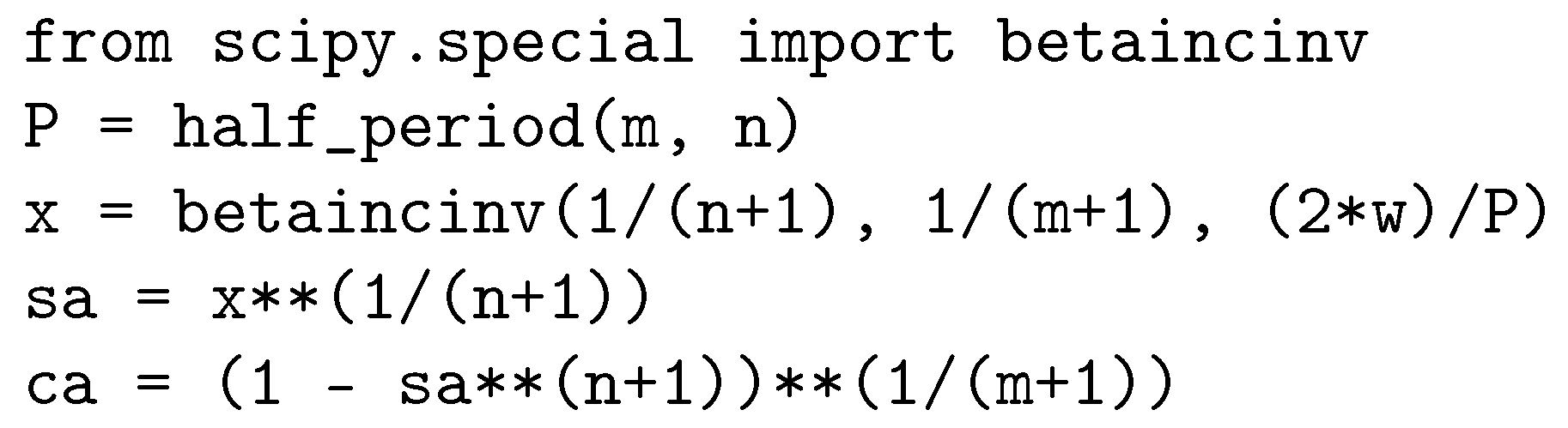
The essential part of the numerical implementation is shown below. The function betaincinv (inverse regularized incomplete beta function) is provided by the SciPy library. The numerical computation of $sa(n,m,\omega )$ and $ca(m,n,\omega )$ is presented in Figure 3.

The resulting values of $sa(n,m,\omega )$ and $ca(m,n,\omega )$ are then used in the numerical evaluation of Ateb-transform coefficients, as described in Section 4.2.

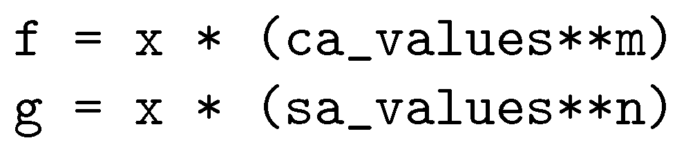
The construction of integrands used for numerical integration is shown in Figure 4.

To obtain numerical approximations of $A(m,n,\omega )$ and $B(n,m,\omega )$, we apply the trapezoidal rule:

$$A(m,n,\omega )\approx {\displaystyle \frac{\Delta t}{2}}\left(f_0\left(\omega \right)+2\sum _{i=1}^{N-1}{f}_i\left(\omega \right)+f_N\left(\omega \right)\right),$$

$$B(n,m,\omega )\approx {\displaystyle \frac{\Delta t}{2}}\left(g_0\left(\omega \right)+2\sum _{i=1}^{N-1}{g}_i\left(\omega \right)+g_N\left(\omega \right)\right).$$

The trapezoidal integration scheme is illustrated in Figure 5.

The inverse transform is given by

$$x(m,n,t)={\displaystyle \frac{1}{2\Pi (m,n)}}{\int }_{-\infty }^{\infty }\left[A(m,n,\omega )\mathrm{ca}(m,n,\omega t)+B(n,m,\omega )\mathrm{sa}(n,m,\omega t)\right]d\omega .$$

Since this integral is taken over an unbounded frequency domain, it is replaced in practice by a truncated interval

$$[-\Omega ,\Omega ].$$

Next, we introduce a uniform frequency grid:

$${\omega }_k=-\Omega +k\Delta \omega ,k=0,1,\dots ,K,\Delta \omega ={\displaystyle \frac{2\Omega }{K}}.$$

Due to the even symmetry of the integrand, the numerical implementation restricts the integration domain to the interval $[0,\Omega ]$.

For fixed t, we compute the integrand values

$$H_k\left(t\right)=A(m,n,{\omega }_k)\mathrm{ca}(m,n,{\omega }_{k}t)+B(n,m,{\omega }_k)\mathrm{sa}(n,m,{\omega }_{k}t).$$

Applying the trapezoidal rule yields the approximation

$$x(m,n,t)\approx {\displaystyle \frac{1}{\Pi (m,n)}}{\displaystyle \frac{\Delta \omega }{2}}\left(H_0\left(t\right)+2\sum _{k=1}^{K-1}{H}_k\left(t\right)+H_K\left(t\right)\right).$$

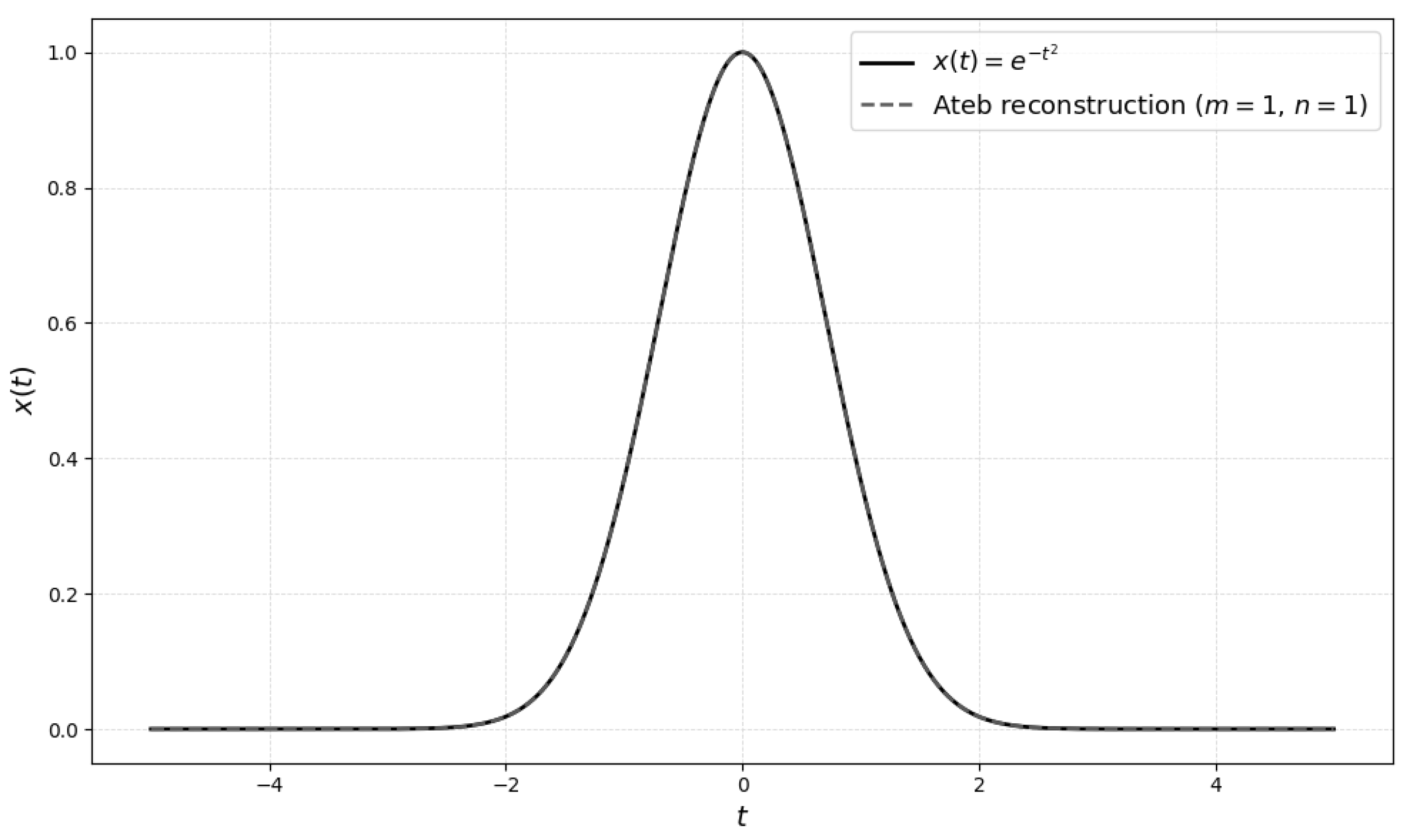
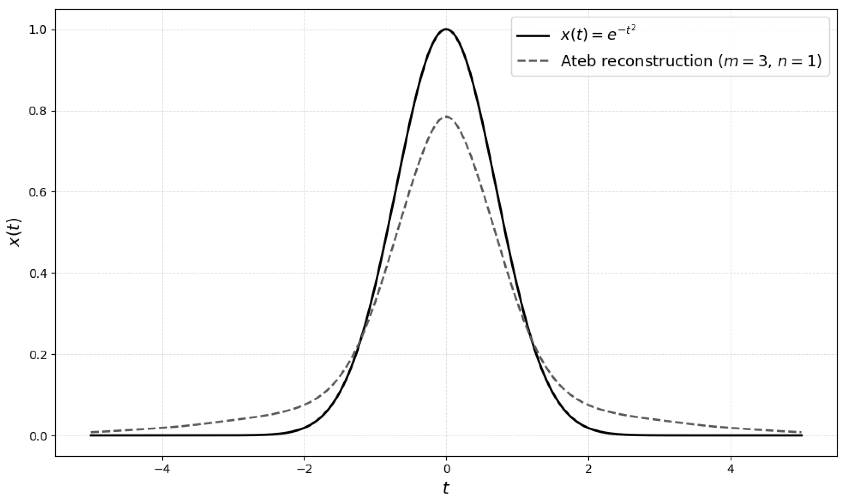
The resulting approximation is then compared with the analytical form of the test function, which provides a basic measure of the numerical accuracy of Ateb-transform implementation.

The illustrations of the algorithm’s performance, obtained for a fixed set of parameters, are presented in Figure 6 and Figure 7.

5. Conclusions

The idea of the Fourier transform was used to construct the Ateb-transform based on periodical Ateb-functions Ateb-cosine $\mathrm{ca}(m,n,\omega t)$ and Ateb-sine $\mathrm{sa}(n,m,\omega t)$; the Ateb-transform algebraic properties were described and proven. An algebra based on the usual addition of functions and multiplication in the form of convolutions was created, together with hypergroups of shift operators. The obtained results show that the Ateb-transform is a natural generalization of the Fourier transform. The Ateb-transform has a complete algebraic structure that includes

• The convolution operation;
• The hypergroup of generalized shift operators;
• The isometry Ateb-transform in $L^2\left(R\right)$;
• Parseval identity;
• Better describes nonlinear oscillatory motions than harmonic analysis;
• Enables constructing new methods for spectral signal processing.

Analytical theorems: additivity and convolution theorems are proved. A numerical algorithm for calculating direct and inverse Ateb-transforms is proposed. The proven properties are illustrated numerically by examples of elementary functions. The application of the obtained results to problems of modeling nonlinear oscillations is discussed. The obtained results confirm that Ateb-functions can be used for modeling oscillatory systems but with advantages for significantly nonlinear oscillations. In future research, Ateb-analysis can be used in telecommunications, filtering, spectral compression of signals, and cryptographic schemes.