Frozen Seismic Foundation Features and Well Log Fusion for Fluid Migration Favorability Ranking

Abstract

Fluid migration screening requires the integration of seismic structure and well log response. This study develops a multimodal framework for ranking an attribute-derived fluid migration favorability proxy from paired local seismic patches and well log windows in the F3 survey. The framework couples frozen seismic foundation model (SFM) features with a trainable well log token encoder and evaluates pooled concatenation, cross attention, and learned query fusion for multimodal integration. Under sample-stratified evaluation across three random seeds, frozen SFM features with learned query fusion achieved the highest observed normalized discounted cumulative gain at rank 20 (nDCG@20) of 85.15%, exceeding the best single-modality baseline by 3.95 percentage points. The results support combining pretrained seismic representations with well log evidence to prioritize intervals in the F3 benchmark.

1. Introduction

Fluid migration screening prioritizes subsurface intervals whose structural and petrophysical evidence is consistent with migration pathways. Seismic discontinuities, fault patterns, gas-chimney signatures, and amplitude anomalies provide spatial evidence, while borehole measurements describe local depth-dependent properties [1,2]. Because these observations differ in spatial support, sampling geometry, and noise, a screening model must combine laterally continuous seismic context with high-resolution well-log response.

Learning-based seismic interpretation has established reproducible models for structural targets such as faults [3], and seismic-to-well sequence models show how sparse well control can constrain predictions from seismic observations [2]. Domain-specific representation learning extends this approach by pretraining seismic encoders on larger unlabeled collections before adapting them to labeled tasks [4,5]. The open-source seismic foundation model (SFM) used here produces contextual tokens from local seismic images [6]. Freezing that backbone concentrates task-specific learning in the well-log encoder, cross-modal fusion module, and prediction head.

We evaluate frozen SFM transfer on an F3 benchmark of paired seismic patches and well-log windows with a continuous, attribute-derived fluid migration favorability score. F3 was selected because its public marine 3D seismic data and associated wells permit reproducible seismic–log pairing within one survey [7]. The experiments separate three questions: whether paired modalities improve ranking over either modality alone, how frozen SFM features compare with a CNN trained from the downstream samples, and how pooled concatenation, cross attention, and learned query fusion behave under the same task protocol.

We formulate fluid migration screening as paired seismic–well ranking and adapt fixed pretrained seismic representations through lightweight cross-modal learning. The contributions are as follows:

• We formulate fluid migration screening as continuous ranking of paired local seismic patches and well-log windows. This formulation combines the complementary spatial and depth-dependent evidence available for each sample.
• We develop a parameter-efficient transfer framework that keeps the seismic foundation model frozen, encodes well-log intervals with a trainable token encoder, and aligns the two modalities at the representation level. The framework isolates downstream adaptation from expensive seismic-backbone fine tuning.
• We establish a controlled comparison of representation source and fusion depth by evaluating single-modality models, a trainable CNN seismic baseline, frozen SFM features, pooled concatenation, cross attention, and learned query fusion under one ranking protocol. This design distinguishes the effect of multimodal evidence from the effect of pretrained seismic features and token-level interaction.
• We evaluate the framework with ranking measures that reflect a prioritization workflow. Among the evaluated configurations, frozen SFM features with learned query fusion achieved the highest observed nDCG@20 mean. The analysis provides fluid migration ranking evidence for the F3 survey.

2. Related Work

2.1. Seismic Interpretation and Geophysical Representation Learning

Seismic interpretation traditionally turns dense reflection data into attributes that make discontinuities, stratigraphic geometries, and amplitude anomalies easier to compare across an area [1]. This attribute-centered practice is important for fluid-migration screening because faults, chimneys, shallow gas, and anomalous amplitudes provide complementary evidence of migration. Early deep-learning studies shifted part of this work from attribute inspection to supervised pattern recognition, especially when synthetic seismic data could provide dense structural labels for fault segmentation [3]. At the same time, well-log facies benchmarks made subsurface learning problems more reproducible by turning interpretation tasks into shared machine-learning comparisons [8]. Seismic-to-well inversion studies also showed that sequence models can use sparse well control to constrain predictions made from seismic traces [2]. These lines of work establish the two ingredients that matter for this paper: seismic images contain spatial evidence for migration pathways, and well logs provide localized depth-dependent constraints.

Foundation models change the question from how to train a model for one labeled interpretation task to how to reuse a representation learned from larger unlabeled data. Recent geophysical surveys argue that exploration geophysics is well suited to this shift because the field has large unlabeled volumes, heterogeneous sensing modalities, and limited task-specific annotation [4]. In seismic interpretation, masked-autoencoder pretraining has been shown to produce domain-specific representations that can transfer better than natural-image pretraining for downstream tasks [5]. Promptable geobody interpretation extends this idea by combining a vision foundation backbone with multimodal prompts so that the same model can delineate different seismic bodies across surveys [9]. Generative seismic foundation modeling pushes the representation problem toward processing, where a single pretrained model can support denoising, interpolation, backscattered-noise attenuation, and low-frequency extrapolation [10]. Transfer performance depends on the pretraining objective, backbone, data distribution, and downstream adaptation strategy [11]. This motivates our comparison of frozen seismic representations and task-trained features within a shared seismic–well ranking protocol. The recent Geophysics perspective similarly frames foundation models for exploration geophysics as emerging infrastructure that should be tested against task-specific geological objectives [4].

Seismology foundation models provide a parallel setting for evaluating reusable seismic representations across tasks, scales, and acquisition contexts. SeisCLIP uses multimodal contrastive pretraining to connect seismic spectra with event-level metadata for general-purpose feature extraction [12]. SeisT shows that a Transformer backbone can serve as a shared model for earthquake detection, phase picking, and magnitude estimation [13]. SeisLM treats waveform records as language-like sequences and pretrains on large open collections before downstream adaptation [14]. The NCS model family highlights the value of large basin-specific corpora when the goal is transfer to seismic interpretation benchmarks [15]. U-Trans further suggests that waveform foundation models can improve downstream earthquake tasks across training-distribution boundaries [16]. These studies motivate specifying the target task, evaluation domain, and adaptation path in seismic–well ranking.

2.2. Foundation Encoders Beyond Seismic Data

The architectural choices in this paper also draw on representation-learning work outside geophysics. The Transformer made token-level self-attention a general mechanism for modeling long-range interactions without recurrence [17]. Vision Transformers then showed that an image can be decomposed into patch tokens, which makes 2D seismic windows naturally compatible with token-based encoders [18]. DINOv2 demonstrated that large self-supervised visual encoders can provide robust off-the-shelf features across diverse downstream tasks [19]. Foundation-model research describes how pretrained representations can support downstream tasks across data domains [20]. In our framework, the frozen SFM supplies seismic tokens, and ranking performance measures their contribution in the F3 task.

Remote sensing and Earth observation offer another nearby analogy for geophysical foundation models. These fields also combine spatial structure, sensor heterogeneity, large unlabeled archives, and limited task-specific labels. A recent survey of remote-sensing foundation models catalogs vision, vision-language, and large-language-model approaches for Earth observation tasks [21]. A vision-foundation-model survey in remote sensing shows that contrastive learning and masked autoencoding are common pretraining choices for spatial Earth data [22]. Multimodal Earth-observation work highlights cross-modal integration as a key capability for foundation models [23]. SkySense provides a concrete example of large-scale multimodal pretraining over optical and synthetic-aperture-radar temporal sequences [24]. Prithvi WxC illustrates how masked reconstruction and forecasting can be combined for weather and climate foundation modeling [25]. These multimodal geoscience examples motivate a compact mechanism for aligning pretrained spatial tokens with well-log measurements.

2.3. Well-Log Sequence Modeling and Seismic–Well Integration

Well logs provide depth-indexed sequence evidence that complements laterally continuous seismic images. Local curve shape, inter-curve covariance, and stratigraphic position can be more informative than any individual sample value, which makes sequence modeling a natural fit. Sequence-based generative models have recently been used to generate and impute well-log data when missing intervals or limited logging suites reduce data completeness [26]. A well-log foundation model proposes tokenization, masked-token modeling, and stratigraphy-aware contrastive learning for multi-task cross-well interpretation [27]. Promptable well-log foundation modeling further suggests that masked autoencoding can scale to large well-log corpora and support downstream formation-top interpretation [28]. Conditional generative well-log imputation has also been combined with swarm optimization and seismic velocity constraints to preserve geological consistency [29]. Recent seismic–well velocity modeling uses masked-autoencoder pretraining before fine-tuning with well labels, which is close in spirit to the frozen-feature transfer evaluated here [30]. These studies motivate the well-log token encoder in our framework, but our target differs from log reconstruction or velocity prediction because the supervision is a continuous fluid migration favorability score.

2.4. Fusion, Ranking, and Imbalanced Evaluation

The final issue is how to connect a frozen seismic encoder to a trainable well-log token encoder through efficient cross-modal fusion. Masked autoencoders provide the reconstruction-based pretraining logic behind the seismic foundation branch used in this paper [31]. BLIP-2 motivates a compact query module that can extract task-relevant information from a frozen visual encoder while leaving the backbone unchanged [32]. This idea is useful for our setting because the trainable module can learn how much seismic evidence to request from fixed SFM tokens before combining it with well-log tokens. Recent RGB–thermal aerial perception work similarly combines pretrained visual representations with adaptive cross-modal fusion, although its semantic-segmentation task and sensing modalities differ from the seismic–well ranking setting considered here [33].

Evaluation also matters because fluid-migration screening is closer to prioritized review than balanced classification. nDCG is appropriate for this ranking objective because gain-based information-retrieval metrics reward highly relevant items near the top of a list [34]. ROC and precision–recall curves can disagree under class imbalance, motivating the joint use of AUROC and precision–recall metrics for the auxiliary binary test [35]. Precision–recall evaluation is often more informative when positive cases are rare or operational attention is focused on a small candidate set [36].

This paper integrates a frozen seismic representation, a well-log token encoder, and lightweight fusion modules for fluid migration ranking on an F3 paired-sample benchmark. The study evaluates how pretrained seismic features and cross-modal interaction support the prioritization of fluid migration favorability.

3. Materials and Methods

3.1. Model Framework

The computational experiments used Python 3.10.4, PyTorch 2.10.0+cu128, CUDA 12.8, NumPy 2.2.6, pandas 2.3.3, scikit-learn 1.7.2, SciPy 1.15.3, and timm 0.3.2.

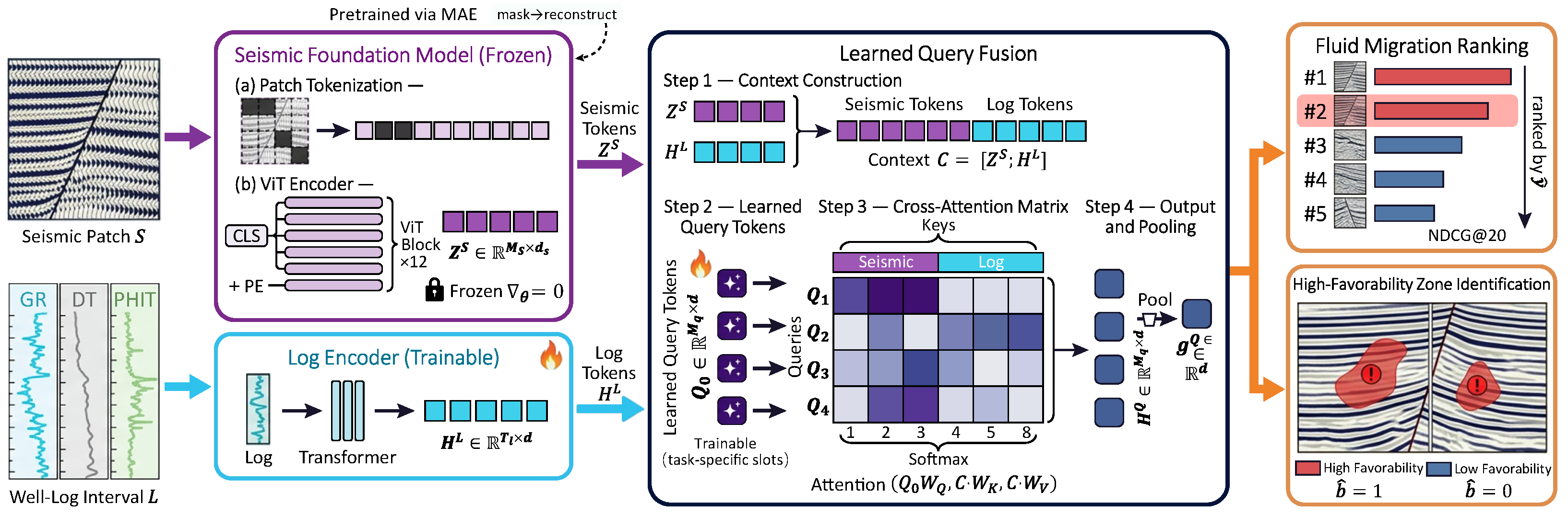
Figure 1 illustrates the framework. A frozen SFM supplies seismic tokens, a trainable two-layer Transformer encodes each well-log window, and one of three fusion modules produces the representation used by the prediction head. A paired sample contains a local seismic cube, a well-log interval, a continuous fluid migration favorability score, a thresholded auxiliary label, and F3 location metadata.

The complete data object and input shapes are defined in Equation (1):

$$\begin{array}{cc}\hfill \mathcal{D}& ={\left\{({\mathbf{S}}_i,{\mathbf{L}}_i,y_i,{\mathbf{m}}_i)\right\}}_{i=1}^N,\hfill \\ \hfill {\mathbf{S}}_i& \in {\mathbb{R}}^{C_s\times D_s\times H_s\times W_s},\hfill \\ \hfill {\mathbf{L}}_i& =[{\mathsf{\ell }}_{i,1};\dots ;{\mathsf{\ell }}_{i,T_l}]\in {\mathbb{R}}^{T_l\times C_l},\hfill \\ \hfill y_i& \in [0,1],b_i^{\left(s\right)}\in \{0,1\}\hfill \end{array}$$

(1)

Equation (1) fixes the notation used by the rest of the paper. The index i denotes one valid paired sample and N is the number of such samples. In the implemented benchmark, ${\mathbf{S}}_i$ is a $1\times 32\times 32\times 32$ local seismic cube. The log matrix ${\mathbf{L}}_i$ is an ordered interval of $T_l=256$ positions with six normalized curves. The target $y_i\in [0,1]$ is the continuous fluid migration favorability score described in Section 4.1, and $b_i^{\left(s\right)}\in \{0,1\}$ is the seed-specific thresholded auxiliary label in Equation (13). The metadata vector ${\mathbf{m}}_i$ stores well identity, inline and crossline position, and interval bounds for analysis and splitting.

This notation also defines the controlled comparison. Every model family receives the same sample set, uses the same train, validation, and test protocol, and predicts the same primary target. The well-log model uses the token encoder, the seismic models use the seismic branch, CNN fusion models learn seismic features from the downstream samples, and SFM fusion models use a frozen seismic foundation encoder. The experiment evaluates representation and fusion configurations with fixed target definitions.

Figure 1 gives the visual overview, and the mathematical pipeline follows the same order. First, a seismic branch converts ${\mathbf{S}}_i$ into seismic tokens. Second, the well-log token encoder converts ${\mathbf{L}}_i$ into log tokens. Third, a fusion module produces a compact multimodal vector. Finally, a prediction head estimates a continuous score for ranking. The auxiliary binary analysis uses a separate thresholded target. Keeping the SFM encoder frozen enables a controlled comparison of pretrained seismic representations and trainable CNN representations under the same downstream protocol.

3.2. SFM Seismic Branch

The SFM branch uses the open-source Seismic Foundation Model implementation by Sheng et al. [6]. The released repository implements a masked-autoencoder architecture with a Vision Transformer backbone, following the same high-level design used in MAE-style visual pretraining but adapted to seismic images. The code uses a patch embedding layer, Transformer blocks, fixed two-dimensional sine–cosine positional embeddings, a class token, random per-sample masking, a decoder with mask tokens, and a reconstruction loss on masked patches.

For a seismic image with patch size P, the encoder first converts the image into a sequence of patch tokens, as expressed in Equation (2):

$${\mathbf{E}}_i^S=[{\mathbf{x}}_{i,1}^S{\mathbf{W}}_{\mathrm{patch}}^S+{\mathbf{p}}_1^S;\dots ;{\mathbf{x}}_{i,M_s}^S{\mathbf{W}}_{\mathrm{patch}}^S+{\mathbf{p}}_{M_s}^S]\in {\mathbb{R}}^{M_s\times d_s},M_s={\displaystyle \frac{H_s{W}_s}{P^2}}$$

(2)

Equation (2) describes the tokenization step. The vector ${\mathbf{x}}_{i,j}^S\in {\mathbb{R}}^{C_s{P}^2}$ is the flattened seismic patch at spatial patch index j, ${\mathbf{W}}_{\mathrm{patch}}^S$ is the patch projection matrix, and ${\mathbf{p}}_j^S$ is the positional embedding attached to patch j. The value $M_s$ is the number of seismic tokens produced from one image, and $d_s$ is the SFM embedding dimension. For each ${32}^3$ cube, the extraction adapter takes the three orthogonal center slices, standardizes each slice independently, and resizes it bilinearly to $224\times 224$. SFM Base 224 returns all 197 encoder tokens per view, including the class token, giving a frozen feature tensor of $591\times 768$ per sample. The expression for $M_s$ assumes that both spatial dimensions are divisible by P.

SFM pretraining then hides a large random subset of those tokens and trains the model to reconstruct the missing seismic patches from the visible context, as formulated in Equation (3):

$${\mathcal{M}}_i\subset \{1,\dots ,M_s\},|{\mathcal{M}}_i|\approx \rho M_s,{\mathcal{L}}_{\mathrm{MAE}}={\displaystyle \frac{1}{|{\mathcal{M}}_i|}}\sum _{j\in {\mathcal{M}}_i}{\parallel {\widehat{\mathbf{x}}}_{i,j}^S-{\mathbf{x}}_{i,j}^S\parallel }_2^2$$

(3)

Equation (3) gives the reconstruction objective that motivates SFM transfer. The set ${\mathcal{M}}_i$ contains masked patch indices for sample i, and $\rho$ is the masking ratio. The vector ${\widehat{\mathbf{x}}}_{i,j}^S$ is the decoder reconstruction of the masked patch, while ${\mathbf{x}}_{i,j}^S$ is the original patch target. The loss averages squared reconstruction error over masked patches. This matters for geology because the encoder infers missing seismic texture from surrounding visible structure, emphasizing reflector continuity, local discontinuity, and texture context.

For downstream fluid-migration ranking, the decoder and pretraining loss are not used. The pretrained encoder is treated as a fixed transformation from a seismic patch to contextual seismic tokens, which is stated in Equation (4):

$${\mathbf{Z}}_i^S=F_{\theta }^{\mathrm{SFM}}\left({\mathbf{S}}_i\right),{\mathbf{Z}}_i^S\in {\mathbb{R}}^{M_s\times d_s},{\nabla }_{\theta }{\mathcal{L}}_{\mathrm{down}}=\mathbf{0}$$

(4)

Equation (4) states the freezing assumption explicitly. The function $F_{\theta }^{\mathrm{SFM}}$ is the pretrained SFM encoder, $\theta$ denotes its pretrained weights, and ${\mathbf{Z}}_i^S$ is the matrix of contextual seismic tokens. The zero gradient condition means that backpropagation updates the projection, fusion, and prediction modules, but not the SFM backbone. This design reduces the trainable parameter count and makes the experiment a test of frozen representation transfer.

The SFM token dimension is not required to match the hidden size used by the log encoder or fusion modules. A trainable projection therefore maps the frozen SFM tokens into the shared fusion space, as given in Equation (5):

$${\overline{\mathbf{H}}}_i^S={\mathbf{Z}}_i^S{\mathbf{W}}_S+{\mathbf{1}}_{M_s}{\mathbf{b}}_S^{\top },{\overline{\mathbf{H}}}_i^S\in {\mathbb{R}}^{M_s\times d}$$

(5)

Equation (5) defines the only trainable seismic-side transformation in the frozen-SFM branch. The matrix ${\mathbf{W}}_S\in {\mathbb{R}}^{d_s\times d}$ maps SFM embeddings into the shared hidden dimension d, and ${\mathbf{b}}_S\in {\mathbb{R}}^d$ is a bias vector. The vector ${\mathbf{1}}_{M_s}$ has length $M_s$ and broadcasts the bias across all seismic tokens. The result ${\overline{\mathbf{H}}}_i^S$ preserves token order but places the SFM representation in the same feature space as the well-log token encoder.

The CNN seismic baseline receives the same ${32}^3$ cube and learns its feature extractor from the downstream training samples. It contains three $3\times 3\times 3$ convolutions with 16, 32, and 128 output channels. Each convolution is followed by batch normalization and GELU, and the first two blocks also apply $2\times 2\times 2$ max pooling. Adaptive average pooling produces a $4\times 4\times 4$ grid, which is reshaped into 64 tokens of dimension 128. In the fusion equations below, ${\mathbf{H}}_i^{S,*}$ denotes the token matrix from the evaluated branch: ${\overline{\mathbf{H}}}_i^S$ for SFM models and the 64-token trainable CNN output for CNN models.

3.3. Well-Log Token Encoder

The well-log token encoder represents each interval as 256 input tokens. The benchmark preprocessing normalizes each curve. Each $256\times 6$ window is padded with one zero-valued channel to match the seven-channel model interface, linearly projected to 128 dimensions, and contextualized by a trainable Transformer encoder, as described in Equation (6):

$${\mathbf{E}}_i^L=[{\tilde{\mathsf{\ell }}}_{i,1}{\mathbf{W}}_L;\dots ;{\tilde{\mathsf{\ell }}}_{i,T_l}{\mathbf{W}}_L],{\mathbf{H}}_i^L=F_{\varphi }^{\log }\left({\mathbf{E}}_i^L\right)\in {\mathbb{R}}^{T_l\times d}$$

(6)

Equation (6) defines the implemented log representation. The vector ${\tilde{\mathsf{\ell }}}_{i,t}\in {\mathbb{R}}^7$ contains the six normalized values and one zero-padded value, and ${\mathbf{W}}_L\in {\mathbb{R}}^{7\times 128}$ is the input projection. The encoder $F_{\varphi }^{\log }$ contains two Transformer encoder layers with four attention heads, a 2048-dimensional feed-forward sublayer, ReLU activation, and dropout of 0.1. Self-attention contextualizes the log values while preserving the 256-token sequence length, without explicit absolute-depth or time-position embeddings. The log-only baseline mean-pools these tokens and applies the same prediction head used by the multimodal models.

3.4. Fusion Modules

The fusion stage is the main modeling test. If the seismic and well-log encoders carry redundant information, pooling their outputs separately should be enough. If their joint geological context is important for fluid migration ranking, token-level interaction should help. We therefore compare three increasingly expressive fusion strategies while keeping the input encoders and prediction heads comparable.

Pooled concatenation is the least interactive strategy, as shown in Equation (7):

$${\mathbf{g}}_i^{\mathrm{cat}}=\left[{\displaystyle \frac{1}{M_s^{*}}}{\displaystyle \sum _{j=1}^{M_s^{*}}}{\mathbf{H}}_{i,j}^{S,*};{\displaystyle \frac{1}{T_l}}{\displaystyle \sum _{t=1}^{T_l}}{\mathbf{H}}_{i,t}^L\right]\in {\mathbb{R}}^{2d}$$

(7)

Equation (7) independently averages the seismic tokens and the log tokens before concatenating the two pooled vectors. Here $M_s^{*}$ is the number of seismic tokens in the evaluated branch and equals $M_s$ for the frozen SFM branch. This module uses global summaries of both modalities for the ranking task.

Cross-attention introduces token-level interaction by using seismic tokens as queries and log tokens as keys and values, as defined in Equation (8):

$$\begin{array}{cc}\hfill {\mathbf{H}}_i^{\mathrm{cross}}& =LN\left(\mathrm{softmax}\left({\displaystyle \frac{\left({\mathbf{H}}_i^{S,*}{\mathbf{W}}_Q\right){\left({\mathbf{H}}_i^L{\mathbf{W}}_K\right)}^{\top }}{\sqrt{d}}}\right)\left({\mathbf{H}}_i^L{\mathbf{W}}_V\right)+{\mathbf{H}}_i^{S,*}\right),\hfill \\ \hfill {\mathbf{H}}_i^{\mathrm{cross}}& \in {\mathbb{R}}^{M_s^{*}\times d},{\mathbf{g}}_i^{\mathrm{cross}}=\mathrm{AvgPool}\left({\mathbf{H}}_i^{\mathrm{cross}}\right)\in {\mathbb{R}}^d\hfill \end{array}$$

(8)

Equation (8) defines the implemented four-head attention interaction. The matrices ${\mathbf{W}}_Q$, ${\mathbf{W}}_K$, and ${\mathbf{W}}_V$ are trainable projections from the shared dimension d to dimension d. The attention output has one row per seismic token; a residual connection adds the original seismic tokens before layer normalization, and AvgPool mean-pools the resulting sequence.

Learned query fusion uses trainable query tokens as a compact information bottleneck over the combined seismic and log context, as expressed in Equation (9):

$$\begin{array}{cc}\hfill {\mathbf{C}}_i& =[{\mathbf{H}}_i^{S,*};{\mathbf{H}}_i^L],\hfill \\ \hfill {\mathbf{H}}_i^Q& =\mathrm{softmax}\left({\displaystyle \frac{\left({\mathbf{Q}}_0{\mathbf{W}}_Q^Q\right){\left({\mathbf{C}}_i{\mathbf{W}}_K^Q\right)}^{\top }}{\sqrt{d}}}\right)\left({\mathbf{C}}_i{\mathbf{W}}_V^Q\right),\hfill \\ \hfill {\mathbf{H}}_i^Q& \in {\mathbb{R}}^{M_q\times d},{\mathbf{g}}_i^Q=\mathrm{AvgPool}\left({\mathbf{H}}_i^Q\right)\in {\mathbb{R}}^d\hfill \end{array}$$

(9)

Equation (9) first forms ${\mathbf{C}}_i$, the concatenated token context containing both seismic and log tokens. The matrix ${\mathbf{Q}}_0\in {\mathbb{R}}^{8\times 128}$ contains eight learned query tokens. A single four-head attention layer maps those queries over the combined seismic and log context, after which mean pooling produces the sample representation. This is a compact query-attention bottleneck inspired by QFormer rather than the multi-stage BLIP-2 Q-Former architecture.

3.5. Prediction Objectives and Ranking Metrics

After encoding and fusion, each model produces one vector ${\mathbf{g}}_i$. For a model using only well logs, ${\mathbf{g}}_i$ is a mean-pooled log representation. For a seismic-only model, it is a mean-pooled seismic representation. For multimodal models, it is one of ${\mathbf{g}}_i^{\mathrm{cat}}$, ${\mathbf{g}}_i^{\mathrm{cross}}$, or ${\mathbf{g}}_i^Q$. The prediction head applies layer normalization, a hidden linear layer with ReLU, and a scalar output layer. Separate instances are trained for continuous ranking and the auxiliary binary analysis, as given in Equation (10):

$$\begin{array}{cc}\hfill {\mathbf{h}}_i& =\mathrm{ReLU}({\mathbf{W}}_1\mathrm{LN}\left({\mathbf{g}}_i\right)+{\mathbf{b}}_1),\hfill \\ \hfill {\widehat{y}}_i& ={\mathbf{w}}_r^{\top }{\mathbf{h}}_i+c_r,{\widehat{p}}_i=\sigma ({\mathbf{w}}_b^{\top }{\mathbf{h}}_i+c_b),\hfill \\ \hfill {\mathcal{L}}_{\mathrm{reg}}& ={\displaystyle \frac{1}{\left|\mathcal{B}\right|}}\sum _{i\in \mathcal{B}}{(y_i-{\widehat{y}}_i)}^2,{\mathcal{L}}_{\mathrm{bin}}=-{\displaystyle \frac{1}{\left|\mathcal{B}\right|}}\sum _{i\in \mathcal{B}}\left[b_i^{\left(s\right)}\log {\widehat{p}}_i+(1-b_i^{\left(s\right)})\log (1-{\widehat{p}}_i)\right]\hfill \end{array}$$

(10)

Equation (10) defines the head and the two objectives. The hidden layer has the same width as its input: 128 for the single-modality, cross-attention, and learned-query models, and 256 for pooled concatenation. The vector ${\mathbf{w}}_r$ and scalar $c_r$ define the regression output, while ${\mathbf{w}}_b$, $c_b$, and the logistic sigmoid $\sigma (·)$ define the binary output. The ranking experiments optimize mean squared error, and the binary experiments optimize unweighted binary cross entropy.

The primary evaluation target is ranking quality. For a ranked list of K test samples, nDCG with linear gain can be computed as shown in Equation (11). Let ${\pi }_{\widehat{y}}$ sort test samples by decreasing predicted score and let ${\pi }_y$ sort them by decreasing target value.

$$\begin{array}{cc}\hfill \mathrm{DCG}@K& ={\displaystyle \sum _{j=1}^K}{\displaystyle \frac{y_{{\pi }_{\widehat{y}}\left(j\right)}}{{\log }_2(j+1)}},\hfill \\ \hfill \mathrm{IDCG}@K& ={\displaystyle \sum _{j=1}^K}{\displaystyle \frac{y_{{\pi }_y\left(j\right)}}{{\log }_2(j+1)}},\hfill \\ \hfill \mathrm{nDCG}@K& ={\displaystyle \frac{\mathrm{DCG}@K}{\mathrm{IDCG}@K}}\hfill \end{array}$$

(11)

Equation (11) defines the metric used for the main claim. ${\pi }_{\widehat{y}}$ gives the model ranking, and ${\pi }_y$ gives the ideal ranking under the continuous fluid migration favorability target. nDCG is appropriate because the intended use case is a review queue in which placing a high-favorability candidate near the top is more valuable than improving the ordering of low-ranked samples.

Two derived quantities separate the experimental claims, as defined in Equation (12):

$$\begin{array}{cc}\hfill {\Delta }_{\mathrm{MM}}& =\mathrm{nDCG}@20\left(F_{\mathrm{seislog}}\right)-\max \{\mathrm{nDCG}@20\left(F_{\log }\right),\mathrm{nDCG}@20\left(F_{\mathrm{seis}}\right)\},\hfill \\ \hfill {\Delta }_{\mathrm{SFM}}& =\mathrm{nDCG}@20\left(F_{\mathrm{SFM}+\mathrm{fusion}}\right)-\mathrm{nDCG}@20\left(F_{\mathrm{CNN}+\mathrm{fusion}}\right)\hfill \end{array}$$

(12)

Equation (12) separates the multimodal comparison from the comparison between the strongest observed frozen SFM and CNN configurations. ${\Delta }_{\mathrm{MM}}$ quantifies the difference between the best seismic and log configuration and the best single-modality model. ${\Delta }_{\mathrm{SFM}}$ captures the configuration-level difference between the leading frozen SFM and CNN models, including their seismic representation and fusion modules.

4. Results

4.1. F3 Data and Experimental Protocol

The F3 dataset comprises public marine three-dimensional seismic data and well information from the offshore of the Netherlands [7]. We chose F3 because its seismic neighborhoods, well-log windows, and location/interval metadata can be aligned within one survey, providing a reproducible setting for seismic–log proxy ranking. The local paired seismic–well index contains 364 rows. After filtering for valid proxy scores, 321 samples remain. The four contributing wells are F03-2 with 91 valid samples, F03-4 with 82, F06-1 with 80, and F02-1 with 68. Well inclusion is determined by the availability of valid paired seismic, log, and target components. Each sample links a seismic neighborhood to a well-log window and metadata describing its well, inline/crossline location, time interval, and horizon interval. Our main evaluation uses sample-stratified splits, so intervals from the same well can appear in both training and test sets.

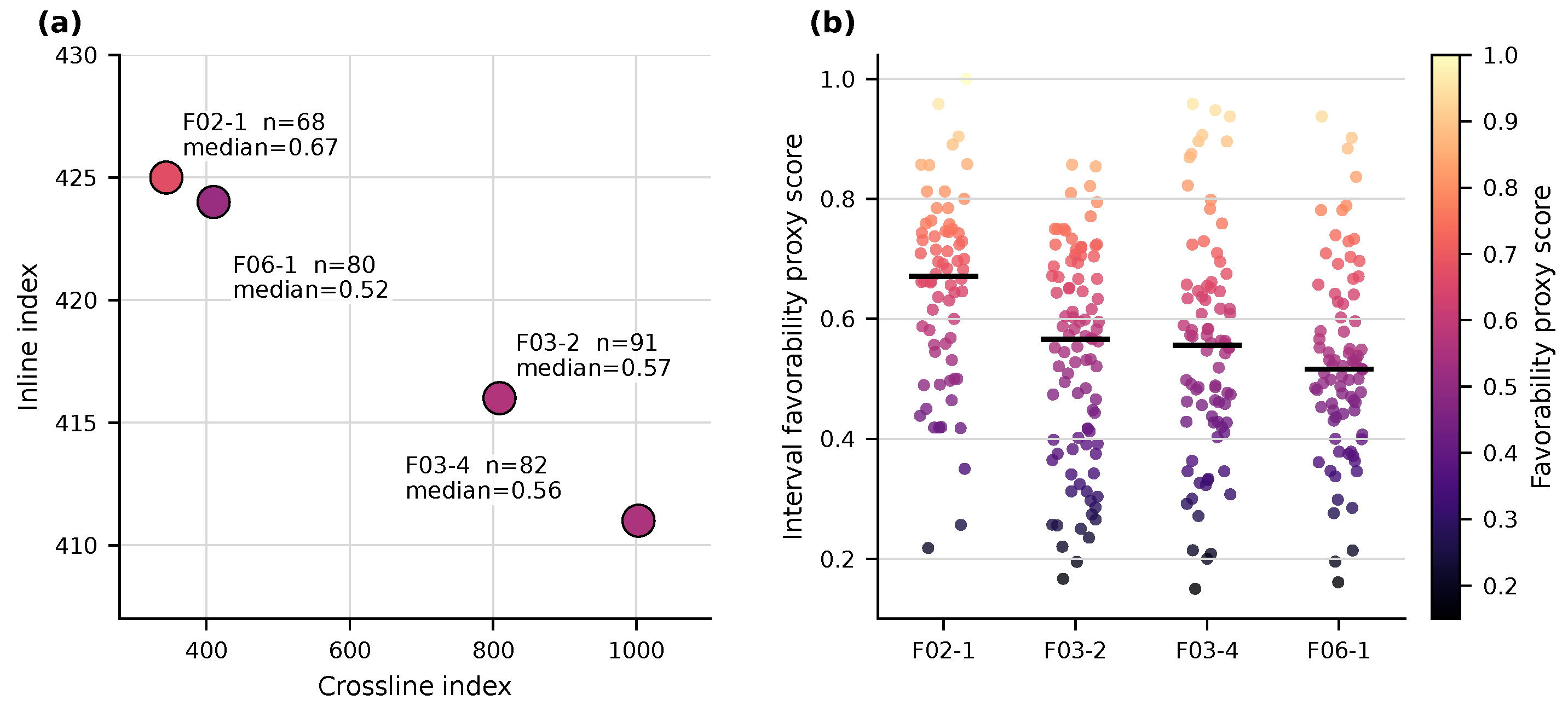
Figure 2 distinguishes the four well coordinates from the multiple scored intervals associated with each coordinate.

The model ranks paired intervals with available seismic context and log windows. The spatial evaluation is concentrated at four well coordinates within F3.

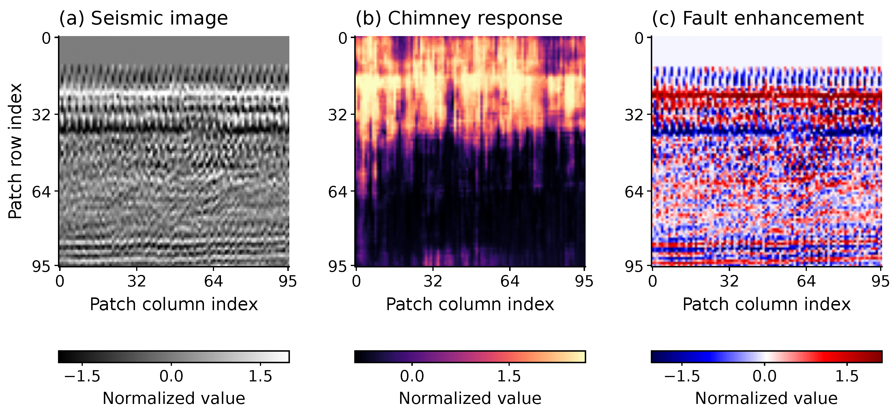
Fluid migration interpretation is motivated by several types of evidence. The seismic image provides reflection geometry and local structural texture. Chimney response highlights vertically disturbed zones that can be associated with migration pathways or gas-related effects. Fault enhancement highlights discontinuities or fault-like features that can provide migration conduits. Well logs provide local petrophysical and elastic responses near the borehole. We visualize this context in Figure 3.

The three panels in Figure 3 illustrate geological context for fluid migration assessment. The seismic image contains stratigraphic and structural texture, while the attribute views and logs provide complementary context. The ranking experiment uses paired seismic and log inputs to predict the favorability proxy defined below.

Each paired sample has a continuous fluid-migration favorability proxy score $y_i\in [0,1]$. The target-generation script ranks available chimney response, fault enhancement, seismic discontinuity, and log-anomaly measures within horizon intervals and combines them with a horizon-position indicator at weights 0.35, 0.30, 0.20, 0.10, and 0.05, respectively; weights for missing components are renormalized. Valid samples require available chimney and fault proxies. The score is an attribute-based index of relative screening priority, with larger values denoting higher favorability. Its components draw on seismic and log information related to the model inputs. Proxy ranks are computed on the paired index before the downstream train/test split, and the benchmark evaluates recovery of this predefined score.

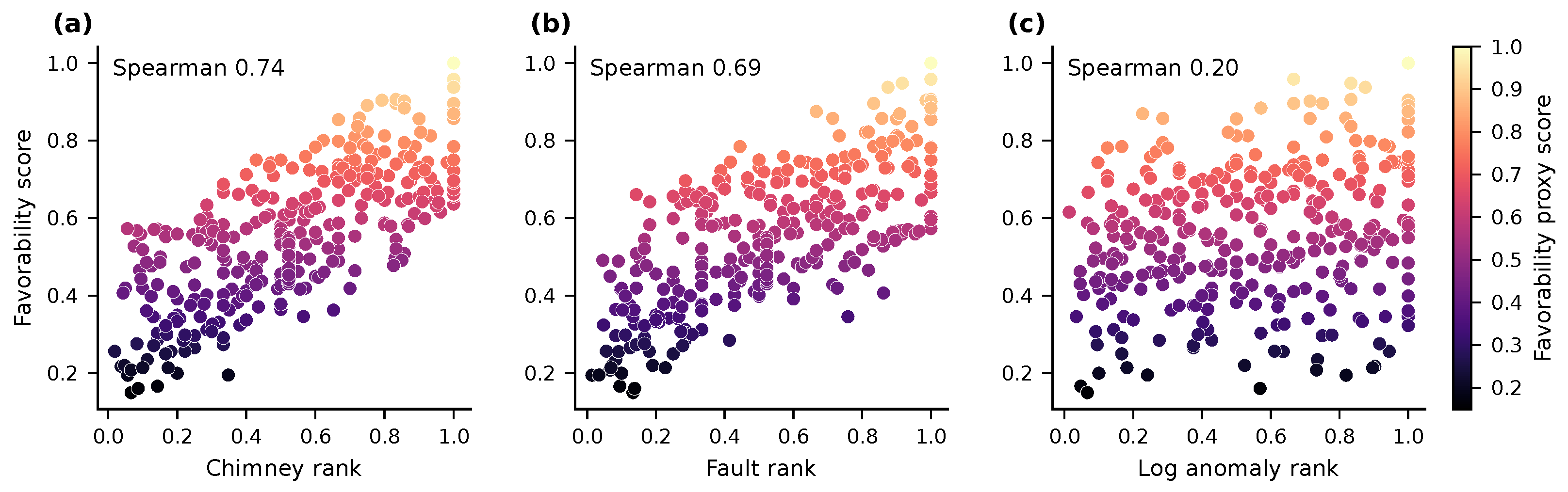
Figure 4 shows the chimney and fault responses used to provide geological context for this target.

The displayed responses indicate structural setting and complement the seismic and well-log evidence used for ranking.

For the auxiliary binary task, the high-favorability cutoff is the upper quartile of the continuous scores in each seed’s training set ${\mathcal{T}}_s$, as shown in Equation (13):

$$b_i^{\left(s\right)}=\mathbb{I}\left(y_i\ge q_{0.75}\left(\{y_j:j\in {\mathcal{T}}_s\}\right)\right)$$

(13)

In Equation (13), $\mathbb{I}(·)$ is the indicator function. The resulting training-score thresholds are 0.68854, 0.69392, and 0.69559 for seeds 0, 1, and 2, respectively; each seed-specific threshold is then applied unchanged to its validation and test samples. The continuous score remains the primary target.

Table 1. F3 fluid migration target summary. Continuous-score statistics use all 321 valid samples; auxiliary binary thresholds are estimated separately from each training split.

Quantity	Value
Sample counts
Rows in paired index	364
Valid continuous-label samples	321
Formal per-seed test size	49
Target distribution
Auxiliary binary training quantile	75th percentile
Training thresholds (seeds 0/1/2)	0.68854/0.69392/0.69559
Continuous-score minimum	15.00%
Continuous-score median	56.25%
Continuous-score mean	56.22%
Continuous-score maximum	100.00%
Continuous-score standard deviation	17.56%

summarizes the sample counts and target distribution for the benchmark.

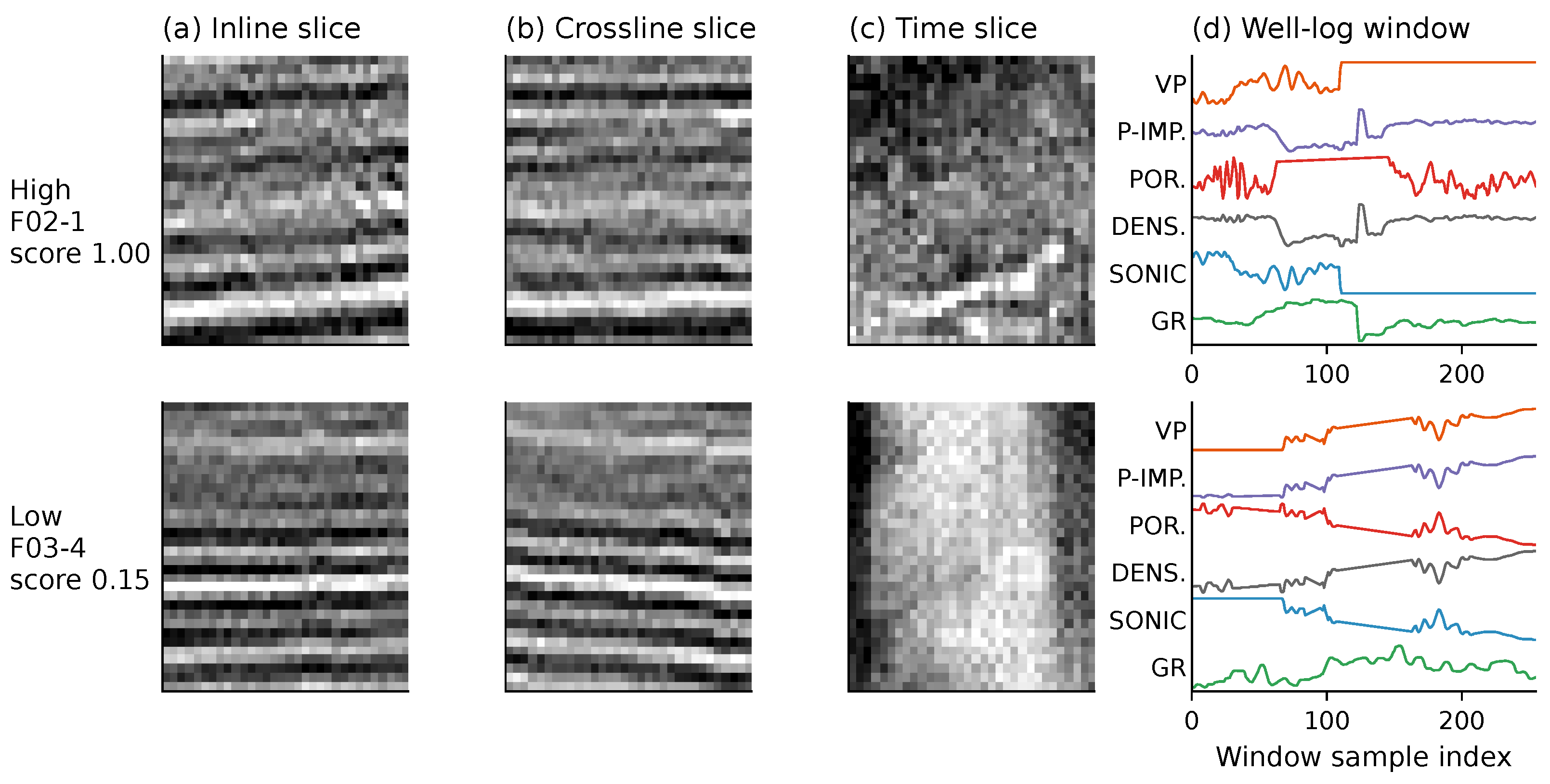
Figure 5 contrasts one high-favorability and one low-favorability paired sample.

The examples have different local seismic textures and well-log responses, but neither modality alone fully defines the target. This motivates the architecture in Section 3: the SFM branch captures seismic texture and structural context, the well-log token encoder captures borehole response, and the fusion module combines them for ranking.

The experiments evaluate the framework in Section 3 as a controlled ranking problem. Each model receives samples from the same F3 paired seismic and well-log benchmark, and the primary target is the continuous fluid-migration favorability score described in this section. The main question is whether a model can rank paired samples so that higher-favorability candidates appear near the top of a review queue.

We compare nine model configurations that vary the input modality, seismic representation, and fusion module. The log-only model removes the seismic branch. The seismic-only CNN removes the well-log token encoder. CNN concatenation, cross attention, and learned query fusion use the task-trained CNN with the corresponding modules in Equations (7)–(9). Feature-only SFM uses the frozen tokens and their trainable projection without logs. The three SFM multimodal configurations combine the same frozen tokens with concatenation, cross attention, or learned query fusion.

Table 2. Implemented model configurations and trainable downstream parameter counts. The frozen SFM backbone is excluded because its features are precomputed and its weights receive no downstream updates.

Seismic Representation	Downstream Configuration	Trainable Parameters
None	Log only	1,203,969
Task-trained CNN	Seismic only	142,628
Task-trained CNN	Concatenation	1,379,364
Task-trained CNN	Cross attention	1,396,004
Task-trained CNN	Learned query fusion	1,396,772
Frozen SFM	Feature only	115,329
Frozen SFM	Concatenation	1,352,065
Frozen SFM	Cross attention	1,368,705
Frozen SFM	Learned query fusion	1,369,473

reports the trainable parameter counts obtained from the saved downstream checkpoints.

The SFM Base 224 checkpoint contains 88,878,336 parameters, of which 85,405,440 belong to the encoder used for feature extraction; the masked-autoencoder decoder is unused downstream. All of these SFM parameters remain frozen. The task-trained CNN seismic encoder contains 125,731 parameters. The comparison therefore contrasts a large pretrained, frozen encoder with a smaller encoder learned from the downstream data.

For each seed, the 321 valid samples are stratified by ranked target quantiles and divided into 224 training samples (69.8%), 48 validation samples (15.0%), and 49 test samples (15.3%). Seeds 0, 1, and 2 determine both this split and model initialization. The continuous target is standardized with the corresponding training-set mean and standard deviation. Every model is trained for 50 epochs with batch size 16 using AdamW, a learning rate of ${10}^{-3}$, weight decay of ${10}^{-4}$, and a gradient-norm limit of 1.0; the reported checkpoint is the final epoch. Frozen SFM representations are precomputed, whereas all CNN weights are learned from the 224 downstream training samples. The models share downstream splits and optimization budgets, with the SFM additionally drawing on its pretraining corpus. The runs were executed on an NVIDIA RTX 3090 Ti GPU.

The two-layer well-log token encoder has 1.19 million trainable parameters, and the multimodal models have 1.35–1.40 million trainable downstream parameters. To measure sensitivity to training-set size, we train the log-only and seismic-only CNN configurations on nested fractions of each training split while holding validation and test samples fixed.

Table 3. Training-size sensitivity for the well-log token encoder and task-trained CNN. Entries are mean [95% confidence interval] in percent over seeds 0, 1, and 2; intervals are t intervals across seeds.

Model	Training Fraction	Train n	nDCG@20 (95% CI)	Spearman (95% CI)	RMSE (95% CI)
Log only	25%	55	77.72 [63.60, 91.85]	18.58 [−22.58, 59.73]	20.08 [17.24, 22.93]
Log only	50%	110	82.49 [66.52, 98.46]	25.65 [−26.30, 77.60]	19.13 [17.09, 21.17]
Log only	75%	169	82.53 [73.66, 91.41]	25.92 [−26.21, 78.06]	17.51 [13.33, 21.69]
Log only	100%	224	81.20 [74.82, 87.59]	27.01 [22.93, 31.08]	17.65 [16.56, 18.75]
Seismic-only CNN	25%	55	79.74 [61.16, 98.31]	20.78 [−39.63, 81.19]	16.69 [15.02, 18.37]
Seismic-only CNN	50%	110	78.01 [65.52, 90.50]	21.79 [−25.06, 68.65]	16.70 [14.83, 18.57]
Seismic-only CNN	75%	169	79.03 [67.75, 90.32]	23.93 [−21.70, 69.55]	16.99 [15.75, 18.23]
Seismic-only CNN	100%	224	78.90 [59.30, 98.50]	21.15 [−24.72, 67.01]	17.23 [16.24, 18.23]

reports the resulting learning curves for the continuous task.

The learning curves show little change between the two largest training fractions under sample-stratified evaluation. In paired comparisons, moving from 75% to 100% of the training split changes log-only nDCG@20 by $-1.33$ percentage points (95% CI [$-14.33$, 11.67]) and seismic-only CNN nDCG@20 by $-0.13$ points (95% CI [$-8.86$, 8.59]). The corresponding intervals for Spearman and RMSE also include zero: log-only changes are 1.09 points [$-52.78$, 54.95] and 0.14 points [$-3.66$, 3.95], while CNN changes are $-2.78$ points [$-5.78$, 0.22] and 0.25 points [$-0.19$, 0.68]. Across the three seeds, the added quarter of training samples produces no detectable gain in these metrics.

We further test whether the log-only result depends on the 2048-dimensional feed-forward sublayer.

Table 4. Well-log encoder capacity sensitivity. Entries are mean [95% confidence interval] in percent over seeds 0, 1, and 2. Parameter counts include the complete log-only model.

Feed-Forward Width	Trainable Parameters	nDCG@20	Spearman	RMSE
256	282,881	80.61 [70.63, 90.59]	27.32 [4.02, 50.62]	18.72 [15.72, 21.71]
512	414,465	81.19 [76.40, 85.98]	32.58 [0.46, 64.70]	17.38 [14.79, 19.97]
2048	1,203,969	81.20 [74.82, 87.59]	27.01 [22.93, 31.08]	17.65 [16.56, 18.75]

reduces that width to 512 and 256 while retaining two Transformer layers, four attention heads, the input projection, and the original optimization protocol.

Relative to the 2048-width encoder, the paired nDCG@20 differences are $-0.59$ points (95% CI [$-5.86$, 4.67]) for width 256 and $-0.01$ points (95% CI [$-6.63$, 6.61]) for width 512. The observed means are similar across widths, while the confidence intervals allow both gains and losses.

Neighboring windows overlap, and sample-stratified splits can share well-specific structure between training and test sets. We therefore assess performance at unseen wells through leave-one-well-out evaluation. Each fold holds out one complete well with 68–91 samples; the remaining wells provide 184–203 training and 46–50 validation samples. For each seed, metrics are averaged over the four held-out wells before the three-seed confidence interval is computed.

Table 5. Leave-one-well-out generalization. Entries are well-macro mean [95% confidence interval] in percent over three seeds. Each test well is absent from both training and validation.

Model	nDCG@20	Spearman	RMSE
Log only	72.81 [67.99, 77.62]	7.41 [−16.56, 31.39]	19.86 [15.43, 24.28]
Seismic-only CNN	72.74 [72.59, 72.89]	16.06 [14.42, 17.70]	19.42 [19.30, 19.55]
SFM feature only	70.38 [65.99, 74.77]	13.48 [4.20, 22.77]	18.96 [18.72, 19.19]

reports this well-macro result.

Compared with sample-stratified evaluation, well-macro nDCG@20 decreases by 8.39 points for log only, 6.16 points for the seismic-only CNN, and 8.91 points for SFM feature only. These decreases quantify the gap between sample-stratified and unseen-well evaluation for the three single-modality models. The training-size and capacity analyses characterize sensitivity within the sampled wells, while the held-out results reveal the additional challenge of generalizing across well locations.

A positional-encoding sensitivity run also tests the implementation choice in Section 3.3. Adding fixed sinusoidal position embeddings to the otherwise unchanged log-only model yields 81.25% nDCG@20, 27.04% Spearman, and 18.22% RMSE, compared with 81.20%, 27.01%, and 17.65%, respectively, without positional embeddings. nDCG@20 and Spearman change little, while RMSE increases, giving no consistent improvement from the added encoding in this experiment.

nDCG@20 is the primary metric because the intended output is a ranked candidate list. We also report nDCG@10 as a complementary shorter cutoff because a 20-sample queue is a substantial fraction of a 49-sample test split. Spearman correlation measures monotone agreement between predicted and target scores. Root mean square error (RMSE) measures absolute score error, and $R^2$ measures explained variance relative to the test set target distribution. The auxiliary binary results use area under the receiver operating characteristic curve (AUROC), area under the precision–recall curve (AUPRC), and balanced accuracy. For readability, all bounded scores and error values are reported as percentages, with RMSE scaled to the normalized 0 to 1 target.

4.2. Main Ranking Results

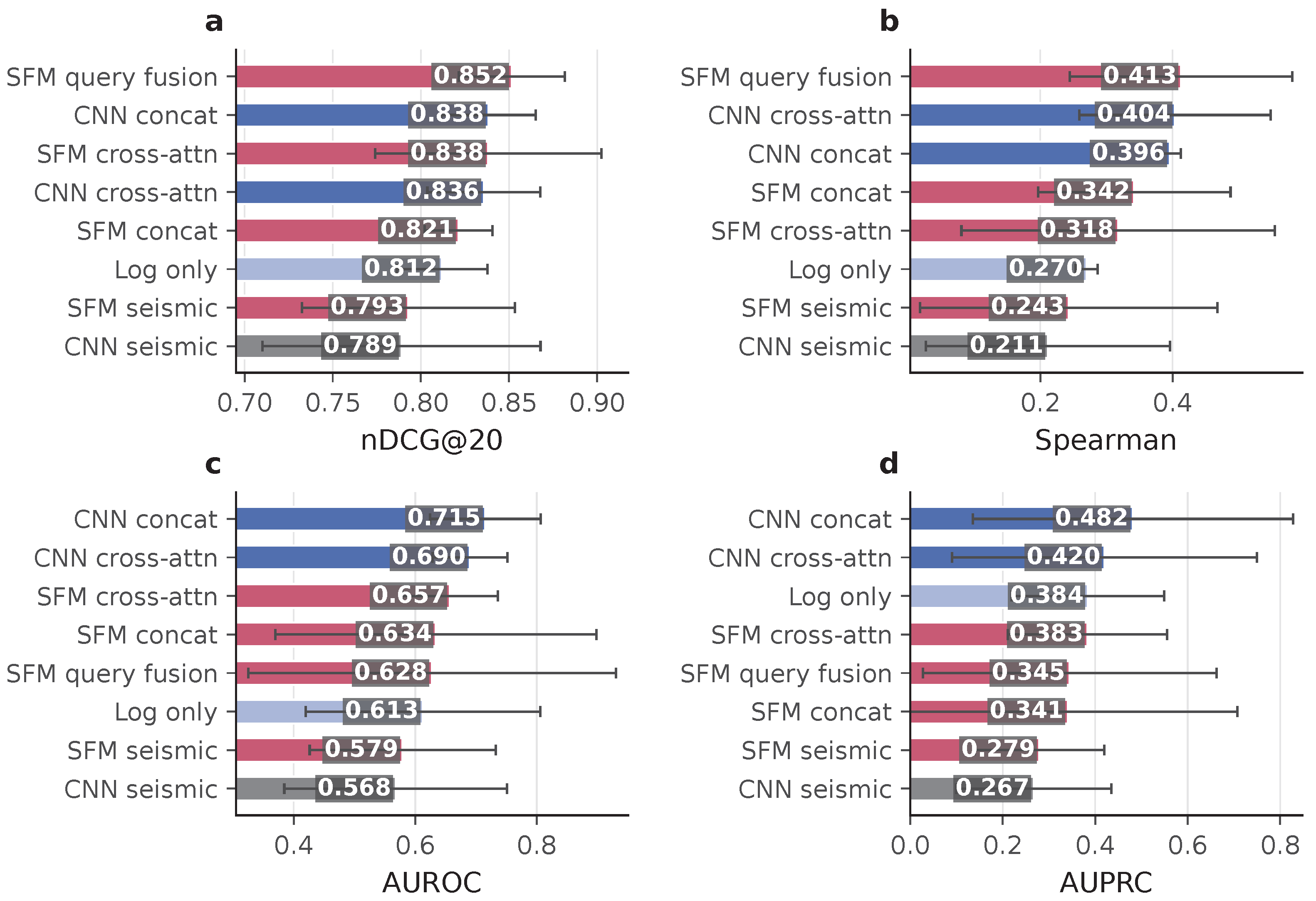
Figure 6 summarizes the eight core configurations, while

Table 6. Regression and ranking results. nDCG entries are mean [95% confidence interval] over three seeds using t intervals; intervals for the bounded nDCG metrics are truncated to [0, 100]. The remaining columns report means. All metrics are percentages, with RMSE scaled to the normalized target.

Family	Model	Test n	nDCG@20, Mean [95% CI]	nDCG@10, Mean [95% CI]	Spearman (%)	RMSE (%)	${\mathit{R}}^2$ (%)
SFM multimodal	SFM learned query fusion	49	85.15 [77.69, 92.62]	80.40 [72.96, 87.83]	41.29	15.60	17.21
CNN multimodal	CNN concatenation	49	83.84 [77.19, 90.49]	83.44 [72.80, 94.09]	39.58	16.06	12.25
SFM multimodal	SFM cross attention	49	83.83 [67.87, 99.79]	81.69 [70.60, 92.78]	31.77	16.58	5.84
CNN multimodal	CNN cross attention	49	83.57 [75.61, 91.53]	80.18 [75.13, 85.22]	40.36	16.10	12.10
CNN multimodal	CNN learned query fusion	49	83.36 [78.90, 87.82]	81.80 [69.00, 94.59]	41.28	16.02	12.50
SFM multimodal	SFM concatenation	49	82.13 [77.37, 86.90]	80.32 [71.46, 89.18]	34.21	16.86	3.14
Log only	Log only	49	81.20 [74.82, 87.59]	80.09 [73.11, 87.06]	27.01	17.65	-5.47
SFM seismic	SFM feature only	49	79.29 [64.27, 94.32]	78.04 [61.94, 94.15]	24.31	16.84	3.81
CNN seismic	Seismic only	49	78.90 [59.30, 98.50]	75.15 [50.11, 100.00]	21.15	17.23	-0.81

also includes the matched CNN learned-query control added for the backbone comparison.

Table 6 reports that the frozen SFM configuration with learned query fusion has the highest observed nDCG@20 mean among the listed configurations. Its reported nDCG@20 is 85.15%, with Spearman correlation of 41.29%, RMSE of 15.60%, and $R^2$ of 17.21%. These measures describe complementary aspects of the continuous task. nDCG@20 evaluates the head of the ranked queue, Spearman evaluates monotone agreement, RMSE evaluates score error, and $R^2$ evaluates explained variation relative to a mean predictor.

The learned query fusion module maps the combined seismic and log token sequences to a compact sample-level representation for the continuous ranking task.

The first experimental pattern concerns multimodal input. The strongest listed single-modality model uses only well logs and reports nDCG@20 of 81.20%, whereas the frozen SFM configuration with learned query fusion reports 85.15%. By Equation (12), the reported difference is ${\Delta }_{\mathrm{MM}}=3.95$. This is the largest listed comparison for the main ranking metric and suggests that combining seismic context with borehole response can improve fluid migration ranking over either modality alone in the evaluated F3 setting.

The second pattern compares the leading frozen SFM and CNN configurations. CNN concatenation reaches nDCG@20 of 83.84%, whereas frozen SFM features with learned query fusion reach 85.15%. The displayed values differ by ${\Delta }_{\mathrm{SFM}}=1.31$, reflecting the combined contribution of the seismic representation and fusion configuration. A matched-fusion comparison holds learned query fusion fixed: the CNN version reaches 83.36%, giving an SFM-minus-CNN difference of 1.80 points (paired 95% CI [$-1.21$, 4.80]). The mean favors the SFM backbone, with uncertainty spanning zero across the three seeds.

nDCG@10 provides a complementary view of the short ranked queue. CNN concatenation reaches 83.44%, whereas frozen SFM features with learned query fusion reach 80.40%. Together with nDCG@20, these results characterize ranking behavior at different review depths.

The final ranking observation concerns calibration versus ordering. SFM feature-only has lower nDCG@20 than log-only, yet its RMSE is slightly better than the log-only RMSE. This pattern shows that score accuracy and prioritized ranking provide complementary views of model performance. For a screening workflow, ranking behavior directly reflects the ordering of high-favorability samples in the review queue.

4.3. Modality and Backbone Analysis

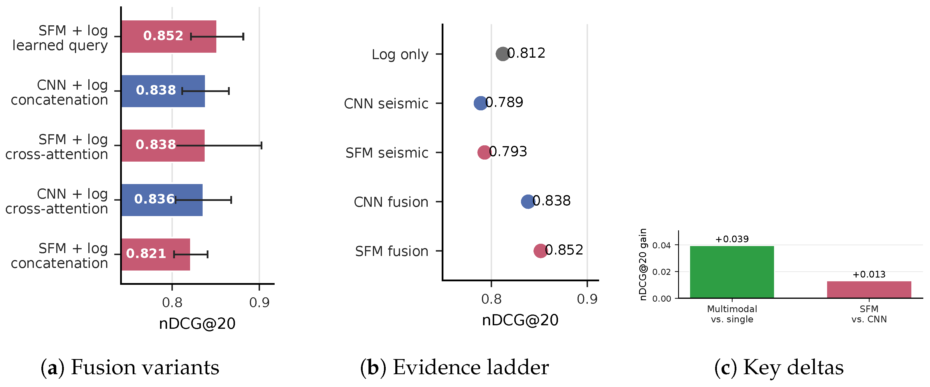
Figure 7 separates the fusion variants, evidence ladder, and principal configuration-level differences.

Figure 7a–c and

Table 7. Key comparisons. Positive differences indicate a higher candidate value than the listed baseline.

Task	Metric	Baseline Configuration	Baseline (%)	Candidate Configuration	Candidate (%)	Difference
Continuous	nDCG@20	Log only	81.20	SFM learned query fusion	85.15	+3.95
Continuous	nDCG@20	CNN concatenation	83.84	SFM learned query fusion	85.15	+1.31
Continuous	nDCG@20	CNN learned query fusion	83.36	SFM learned query fusion	85.15	+1.80
Binary	AUROC	Log only	61.26	CNN concatenation	71.54	+10.28
Binary	AUROC	CNN concatenation	71.54	SFM cross attention	65.71	−5.83
Binary	AUROC	CNN concatenation	71.54	SFM learned query fusion	62.75	−8.79
Binary	AUROC	CNN learned query fusion	65.99	SFM learned query fusion	62.75	−3.23

provides complementary views of the listed comparisons. The evidence ladder begins with the single-modality baselines. The model using only well logs reports 81.20% nDCG@20, the seismic-only CNN reports 78.90%, and frozen SFM features alone report 79.29%. The highest observed nDCG@20 value is reported by a multimodal configuration, which is consistent with complementary seismic and log information in this benchmark.

The comparison between the leading CNN and frozen SFM configurations combines changes in both the seismic representation and fusion module. CNN concatenation reports nDCG@20 of 83.84%, and frozen SFM features with learned query fusion report 85.15%. The additional CNN learned-query control reports 83.36%, isolating the seismic representation while holding the fusion mechanism fixed. The resulting paired SFM-minus-CNN difference is 1.80 nDCG@20 points with a 95% confidence interval of [$-1.21$, 4.80].

The single-modality SFM result is also informative. Feature-only SFM reports nDCG@20 of 79.29%, slightly above seismic-only CNN at 78.90%, while log-only reports 81.20%. The strongest frozen-SFM result occurs when seismic tokens are paired with well-log evidence, highlighting the value of multimodal integration for fluid migration ranking.

4.4. Fusion Strategy and Qualitative Analysis

The frozen SFM variants compare fusion modules while holding the seismic feature source fixed. SFM concatenation reports 82.13% nDCG@20, SFM cross attention reports 83.83%, and SFM learned query fusion reports 85.15%. In this benchmark, the learned-query configuration has the highest observed nDCG@20 mean among the listed frozen-SFM variants.

The frozen SFM encoder produces a token sequence that is summarized by the downstream module. Pooled concatenation, cross attention, and learned query fusion provide progressively different forms of interaction and aggregation. The present results characterize their empirical ranking behavior.

The nDCG@20 confidence intervals in Table 6 overlap across fusion variants, leaving their mean ordering uncertain across splits and seeds.

At nDCG@10, SFM cross attention reaches 81.69%, SFM learned query fusion reaches 80.40%, and SFM concatenation reaches 80.32%. The learned query result is therefore specific to the nDCG@20 evaluation used as the primary metric.

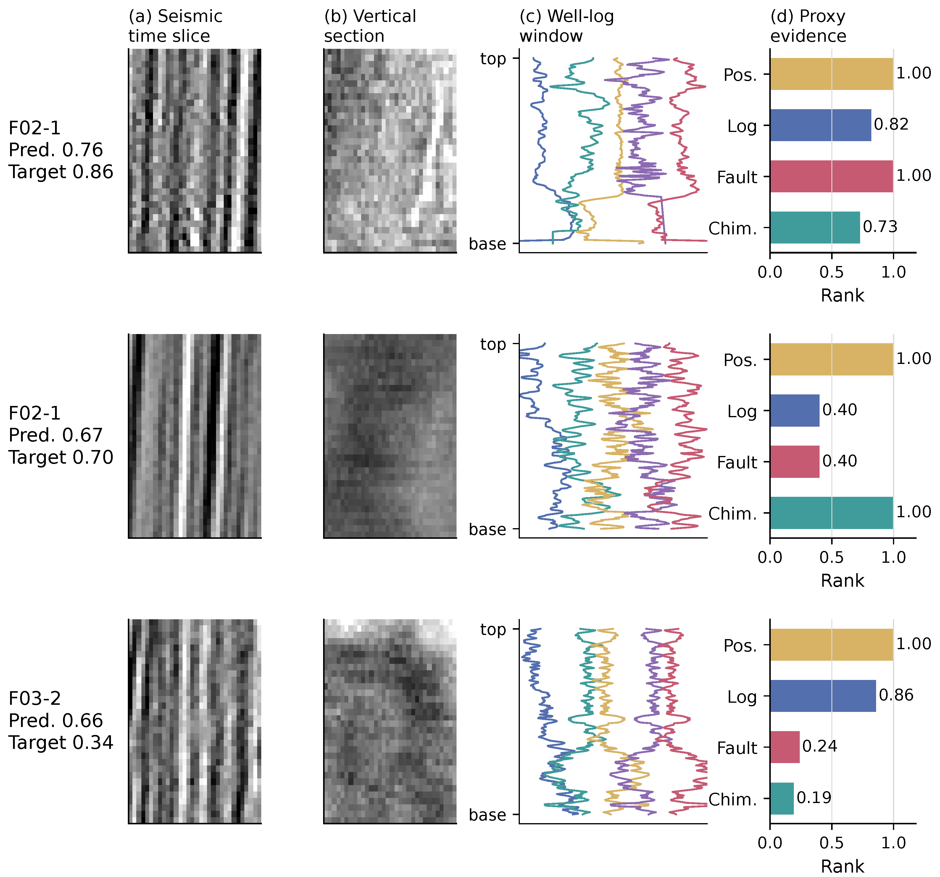
Figure 8 relates representative learned-query predictions to their seismic and well-log inputs.

The illustrated high-score cases connect the seismic structure and log response to the constructed favorability proxy. Chimney and fault views show the corresponding target components.

Some high-favorability samples receive moderate predictions and show mixed seismic and log cues.

The qualitative results also distinguish the ranking and binary tasks. Ranking rewards a model for keeping several intervals with high fluid migration favorability in the upper part of the list. The binary task instead applies the seed-specific training-set threshold in Equation (13). This makes ranking the more direct evaluation for the intended screening workflow.

4.5. Auxiliary Binary Classification

Table 8. Auxiliary binary classification under the per-seed training-set 75th-percentile label protocol. AUROC and AUPRC entries are mean [95% confidence interval] over three seeds using t intervals, truncated to the bounded range [0, 100]. Balanced accuracy is the three-seed mean at the default probability threshold of 0.5. All metrics are percentages.

Family	Model	Seeds	Test n	AUROC, Mean [95% CI]	AUPRC, Mean [95% CI]	Balanced Accuracy, Mean
CNN multimodal	CNN concatenation	3	49	71.54 [62.45, 80.63]	48.16 [13.56, 82.76]	56.02
CNN multimodal	CNN cross attention	3	49	69.00 [62.84, 75.16]	42.03 [9.07, 75.00]	53.00
CNN multimodal	CNN learned query fusion	3	49	65.99 [61.80, 70.17]	42.82 [32.32, 53.33]	54.94
SFM multimodal	SFM cross attention	3	49	65.71 [57.82, 73.60]	38.32 [21.09, 55.55]	49.53
SFM multimodal	SFM concatenation	3	49	63.40 [36.95, 89.85]	34.10 [0.00, 70.76]	48.83
SFM multimodal	SFM learned query fusion	3	49	62.75 [32.49, 93.02]	34.48 [2.75, 66.21]	51.43
Log only	Log only	3	49	61.26 [41.97, 80.56]	38.43 [21.95, 54.91]	52.28
SFM seismic	SFM feature only	3	49	57.93 [42.61, 73.24]	27.95 [13.92, 41.98]	49.53
CNN seismic	Seismic only	3	49	56.78 [38.44, 75.13]	26.72 [9.97, 43.48]	50.00

reports the auxiliary classification results obtained after thresholding the continuous fluid migration favorability score.

CNN concatenation has the highest listed binary AUROC and AUPRC, at 71.54% and 48.16%. The strongest frozen-SFM binary configuration is cross attention, at 65.71% AUROC and 38.32% AUPRC. SFM learned query fusion reaches 62.75% AUROC and 34.48% AUPRC, 8.79 AUROC points below CNN concatenation. Holding learned query fusion fixed narrows the AUROC comparison: CNN learned query fusion reaches 65.99% AUROC and 42.82% AUPRC, so the SFM-minus-CNN differences are $-3.23$ AUROC points (paired 95% CI [$-29.69$, 23.22]) and $-8.34$ AUPRC points ([$-29.77$, 13.09]). The matched binary means favor the CNN backbone, with both paired intervals spanning zero. Table 7 identifies the architectures in the best-configuration and fixed-architecture comparisons.

The learned-query model’s default-threshold balanced accuracy and F1 are 51.43% and 7.41%, respectively. Selecting the decision threshold on the corresponding validation split raises these test means to 61.05% balanced accuracy and 44.06% F1. Its mean Brier score is 16.87%, and its 10-bin equal-width expected calibration error is 8.39%. Threshold adjustment improves the hard-decision metrics while leaving AUROC and AUPRC unchanged below the leading CNN configuration. The results thus distinguish decision-threshold selection from binary discrimination. Under an upper-quartile binary objective and three small training splits, compressing 591 seismic tokens and 256 log tokens through eight learned queries may be harder to optimize than pooling or direct cross attention. The relative contributions of optimization difficulty and overfitting remain unresolved.

5. Conclusions

This study evaluates continuous ranking of an attribute-derived fluid migration favorability proxy using frozen SFM features and a trainable well-log token encoder. The shared protocol separates the effects of modality, seismic representation source, and fusion design. Frozen SFM features with learned query fusion achieve the highest observed nDCG@20 mean in the sample-stratified F3 benchmark. The matched learned-query comparison also favors the SFM backbone in mean continuous ranking, while CNN concatenation leads the auxiliary binary task. These findings support seismic–well fusion for prioritizing the F3 screening proxy and identify fusion choice as a task-dependent design decision.

References

1. Chopra, S.; Marfurt, K.J. Seismic attributes – A historical perspective. Geophysics 2005, 70, 3SO–28SO. [Google Scholar] [CrossRef] [Scilit]
2. Alfarraj, M.; AlRegib, G. Semisupervised sequence modeling for elastic impedance inversion. Interpretation 2019, 7, SE237–SE249. [Google Scholar] [CrossRef] [Scilit]
3. Wu, X.; Liang, L.; Shi, Y.; Fomel, S. FaultSeg3D: Using synthetic data sets to train an end-to-end convolutional neural network for 3D seismic fault segmentation. Geophysics 2019, 84, IM35–IM45. [Google Scholar] [CrossRef] [Scilit]
4. Liu, Q.; Chen, Z.; Ma, J. Foundation models for exploration geophysics. Geophysics 2025, 90, H29–H52. [Google Scholar] [CrossRef] [Scilit]
5. Ordonez, A.; Wade, D.; Ravaut, C.; Waldeland, A.U. Towards a Foundation Model for Seismic Interpretation. In Proceedings of the 85th EAGE Annual Conference and Exhibition; European Association of Geoscientists & Engineers (EAGE): Houten, The Netherlands, 2024; pp. 1–5. [Google Scholar] [CrossRef] [Scilit]
6. Sheng, H.; Wu, X.; Si, X.; Li, J.; Zhang, S.; Duan, X. Seismic foundation model: A next generation deep-learning model in geophysics. Geophysics 2025, 90, IM59–IM79. [Google Scholar] [CrossRef] [Scilit]
7. Society of Exploration Geophysicists. F3 Netherlands; SEG Wiki: Houston, TX, USA, 2026. [Google Scholar]
8. Alaudah, Y.; Michałowicz, P.; Alfarraj, M.; AlRegib, G. A machine-learning benchmark for facies classification. Interpretation 2019, 7, SE175–SE187. [Google Scholar] [CrossRef] [Scilit]
9. Gao, H.; Wu, X.; Liang, L.; Sheng, H.; Si, X.; Gao, H.; Li, Y. A foundation model empowered by a multi-modal prompt engine for universal seismic geobody interpretation across surveys. Inf. Fusion 2026, 125, 103437. [Google Scholar] [CrossRef] [Scilit]
10. Cheng, S.; Harsuko, R.; Alkhalifah, T. A generative foundation model for an all-in-one seismic processing framework. Surv. Geophys. 2025, 46, 1173–1215. [Google Scholar] [CrossRef] [Scilit]
11. Fuchs, F.; Fernandez, M.R.; Ettrich, N.; Keuper, J. Foundation Models For Seismic Data Processing: An Extensive Review. arXiv 2025, arXiv:2503.24166. [Google Scholar]
12. Si, X.; Wu, X.; Sheng, H.; Zhu, J.; Li, Z. SeisCLIP: A seismology foundation model pre-trained by multi-modal data for multi-purpose seismic feature extraction. IEEE Trans. Geosci. Remote Sens. 2024, 62, 5903713. [Google Scholar] [CrossRef] [Scilit]
13. Li, S.; Yang, X.; Cao, A.; Wang, C.; Liu, Y.; Liu, Y.; Niu, Q. SeisT: A foundational deep-learning model for earthquake monitoring tasks. IEEE Trans. Geosci. Remote Sens. 2024, 62, 5908215. [Google Scholar] [CrossRef] [Scilit]
14. Liu, T.; Muenchmeyer, J.; Laurenti, L.; Marone, C.; de Hoop, M.V.; Dokmanic, I. SeisLM: A Foundation Model for Seismic Waveforms. arXiv 2024, arXiv:2410.15765. [Google Scholar]
15. Ordonez, A.; Forgaard, T.J.L.; Wade, D.; Bugge, A.J.; Nese, H.; Waldeland, A.U. The NCS-Model: A seismic foundation model trained on the Norwegian repository of public data. arXiv 2026, arXiv:2603.23211. [Google Scholar]
16. Saad, O.M.; Chen, Y.; Alkhalifah, T. U-Trans: A foundation model for seismic waveform representation and enhanced downstream earthquake tasks. Sci. Rep. 2026, 16, 12657. [Google Scholar] [CrossRef] [Scilit] [PubMed]
17. Vaswani, A.; Shazeer, N.; Parmar, N.; Uszkoreit, J.; Jones, L.; Gomez, A.N.; Kaiser, L.; Polosukhin, I. Attention is All you Need. In Proceedings of the Advances in Neural Information Processing Systems; Curran Associates, Inc.: Red Hook, NY, USA, 2017; pp. 5998–6008. [Google Scholar]
18. Dosovitskiy, A.; Beyer, L.; Kolesnikov, A.; Weissenborn, D.; Zhai, X.; Unterthiner, T.; Dehghani, M.; Minderer, M.; Heigold, G.; Gelly, S.; et al. An Image is Worth 16x16 Words: Transformers for Image Recognition at Scale. In Proceedings of the International Conference on Learning Representations, Virtual, 3–7 May 2021. [Google Scholar]
19. Oquab, M.; Darcet, T.; Moutakanni, T.; Vo, H.; Szafraniec, M.; Khalidov, V.; Fernandez, P.; Haziza, D.; Massa, F.; El-Nouby, A.; et al. DINOv2: Learning Robust Visual Features without Supervision. Trans. Mach. Learn. Res. 2024. Available online: https://openreview.net/forum?id=a68SUt6zFt (accessed on 4 October 2026).
20. Bommasani, R.; Hudson, D.A.; Adeli, E.; Altman, R.; Arora, S.; von Arx, S.; Bernstein, M.S.; Bohg, J.; Bosselut, A.; Brunskill, E.; et al. On the Opportunities and Risks of Foundation Models. arXiv 2021, arXiv:2108.07258. [Google Scholar]
21. Xiao, A.; Xuan, W.; Wang, J.; Huang, J.; Tao, D.; Lu, S.; Yokoya, N. Foundation Models for Remote Sensing and Earth Observation: A Survey. IEEE Geosci. Remote Sens. Mag. 2025, 13, 297–324. [Google Scholar] [CrossRef] [Scilit]
22. Lu, S.; Guo, J.; Zimmer-Dauphinee, J.R.; Nieusma, J.M.; Wang, X.; VanValkenburgh, P.; Wernke, S.A.; Huo, Y. Vision Foundation Models in Remote Sensing: A Survey. IEEE Geosci. Remote Sens. Mag. 2025, 13, 2–27. [Google Scholar] [CrossRef] [Scilit]
23. Hong, D.; Li, C.; Zhang, B.; Yokoya, N.; Benediktsson, J.A.; Chanussot, J. Multimodal artificial intelligence foundation models: Unleashing the power of remote sensing big data in earth observation. Innov. Geosci. 2024, 2, 100055. [Google Scholar] [CrossRef] [Scilit]
24. Guo, X.; Lao, J.; Dang, B.; Zhang, Y.; Yu, L.; Ru, L.; Zhong, L.; Huang, Z.; Wu, K.; Hu, D.; et al. SkySense: A Multi-Modal Remote Sensing Foundation Model Towards Universal Interpretation for Earth Observation Imagery. In Proceedings of the IEEE/CVF Conference on Computer Vision and Pattern Recognition, Seattle, WA, USA, 16–22 June 2024. [Google Scholar] [CrossRef] [Scilit]
25. Schmude, J.; Roy, S.; Trojak, W.; Jakubik, J.; Civitarese, D.S.; Singh, S.; Kuehnert, J.; Ankur, K.; Gupta, A.; Phillips, C.E.; et al. Prithvi WxC: Foundation Model for Weather and Climate. arXiv 2024, arXiv:2409.13598. [Google Scholar]
26. Al-Fakih, A.; Koeshidayatullah, A.; Mukerji, T.; Al-Azani, S.; Kaka, S.I. Well log data generation and imputation using sequence based generative adversarial networks. Sci. Rep. 2025, 15, 11000. [Google Scholar] [CrossRef] [Scilit] [PubMed]
27. Qi, Z.; Yu, Q.; Wang, J.; Zhao, Y.B.; Li, Z.; Lv, W. WLFM: A Well-Logs Foundation Model for Multi-Task and Cross-Well Geological Interpretation. arXiv 2025, arXiv:2509.18152. [Google Scholar]
28. Lasscock, B.; Sansal, A.; Gonzalez, K.; Valenciano, A. Well log foundation model: Making promptable AI models for interpretation. In Proceedings of the SEG/AAPG International Meeting for Applied Geoscience and Energy, Houston, TX, USA, 25–28 August 2025. [Google Scholar] [CrossRef] [Scilit]
29. Qu, F.; Liao, H.; Liu, J.; Wu, T.; Shi, F.; Xu, Y. A novel well log data imputation method with CGAN and swarm intelligence optimization. Energy 2024, 293, 130694. [Google Scholar] [CrossRef] [Scilit]
30. Li, G.; Li, Y.; Huang, J.; Wu, X. A pre-training and fine-tuning paradigm for building a subsurface model. J. Geophys. Eng. 2025, 22, 877–888. [Google Scholar] [CrossRef] [Scilit]
31. He, K.; Chen, X.; Xie, S.; Li, Y.; Dollar, P.; Girshick, R.B. Masked Autoencoders Are Scalable Vision Learners. In Proceedings of the IEEE/CVF Conference on Computer Vision and Pattern Recognition; IEEE: Piscataway, NJ, USA, 2022; pp. 15979–15988. [Google Scholar] [CrossRef] [Scilit]
32. Li, J.; Li, D.; Savarese, S.; Hoi, S.C.H. BLIP-2: Bootstrapping Language-Image Pre-training with Frozen Image Encoders and Large Language Models. In Proceedings of the 40th International Conference on Machine Learning; PMLR: Brookline, MA, USA, 2023; Volume 202, pp. 19730–19742. [Google Scholar]
33. Zhu, C.; Wang, J.; Zhang, L.; Liang, J.; Su, Q.; Li, B. SAM-FuseNet: Segment Anything Guided Multimodal Fusion for RGB–Thermal Aerial Robotic Perception. IEEE Trans. Geosci. Remote Sens. 2026, 64, 5000212. [Google Scholar] [CrossRef] [Scilit]
34. Jarvelin, K.; Kekalainen, J. Cumulated gain-based evaluation of IR techniques. ACM Trans. Inf. Syst. 2002, 20, 422–446. [Google Scholar] [CrossRef] [Scilit]
35. Davis, J.; Goadrich, M.H. The relationship between Precision-Recall and ROC curves. In Proceedings of the Twenty-Third International Conference on Machine Learning; ACM: New York, NY, USA, 2006; pp. 233–240. [Google Scholar] [CrossRef] [Scilit]
36. Saito, T.; Rehmsmeier, M. The Precision-Recall Plot Is More Informative than the ROC Plot When Evaluating Binary Classifiers on Imbalanced Datasets. PLoS ONE 2015, 10, e0118432. [Google Scholar] [CrossRef] [Scilit] [PubMed]
Figure 1. Overall framework of the proposed frozen seismic foundation model and well log fusion network for fluid migration favorability ranking. The framework consists of a frozen seismic foundation model (SFM), a trainable well log encoder, a learned query fusion module, and a prediction head for continuous ranking. Purple and cyan denote seismic and well-log tokens, respectively; red/orange and blue denote high and low favorability, respectively; and the “!” markers identify highlighted high-favorability zones.
Applsci 16 09977 g001
Figure 2. Location and score coverage of the 321 valid paired intervals. (a) Inline–crossline coordinates of the four wells; each marker represents a well, and its color gives the median proxy favorability across that well’s intervals. Sample count and median are printed beside each location. (b) Individual interval-level proxy scores at each well; horizontal bars mark medians. The common color scale maps lower to higher favorability.
Applsci 16 09977 g002
Figure 3. Seismic and attribute context for the proxy target: (a) local seismic image, (b) chimney response, and (c) fault enhancement. The chimney and fault attributes contribute to the weighted target construction.
Applsci 16 09977 g003
Figure 4. Components associated with the constructed favorability proxy. Panels (a–c) show chimney rank, fault rank, and log-anomaly rank against the final weighted score; point color follows the score scale on the right. The component–score associations partly follow from the weighted target construction.
Applsci 16 09977 g004
Figure 5. Examples with high (top row; proxy score 100%) and low (bottom row; proxy score 15%) favorability. Columns (a–d) show inline, crossline, and time seismic slices and the corresponding normalized well-log window. The horizontal log coordinate is the sample index within a 256-point interval, not depth in metres. Curve names and scores are given outside the image panels to avoid obscuring the data.
Applsci 16 09977 g005
Figure 6. Main fluid migration proxy-ranking results for the evaluated model configurations. Panels (a,b) report continuous ranking and score agreement; panels (c,d) report the auxiliary binary metrics. Numeric annotations are placed within the plotting area for legibility.
Applsci 16 09977 g006
Figure 7. Ablation summary. (a) Fusion variants; (b) an evidence ladder in which each colored dot is the mean nDCG@20 of the directly labelled configuration (grey: log only; blue: CNN-based; rose: SFM-based); (c) key configuration-level differences. Confidence intervals for the point estimates in panel (b) are reported in Table 6.
Applsci 16 09977 g007
Figure 8. Representative fluid migration favorability predictions. Examples with high predicted favorability show seismic structure and normalized, horizontally offset log curves. Chimney and fault views provide geological context for the paired samples. In panel (d), gold, blue, rose, and teal bars denote positional, log, fault, and chimney evidence, respectively; bar length gives the normalized evidence rank.
Applsci 16 09977 g008