From Discrete Global Grid Systems to Earth System Spatial Grid: A Review of 3D Extension, Encoding, and Applications

Abstract

As Earth system science moves toward global-domain and multi-sphere coupling, traditional two-dimensional spatial information frameworks can no longer fully meet the integrated spatial computing demands of deep space, deep Earth, and deep ocean applications. Building on research in Discrete Global Grid Systems (DGGS), this paper provides a comprehensive review of Earth System Spatial Grid (ESSG) for three-dimensional Earth system modeling. It focuses on three major categories, namely shell-based, volumetric, and unstructured approaches, and examines their geometric construction, radial extension, and encoding mechanisms. The paper further summarizes representative applications of ESSG in geophysics, space sciences, digital twins, and spatial intelligence, and discusses future challenges including ellipsoid adaptation, international standardization, cloud-native computing, and four-dimensional spatiotemporal extension.

1. Introduction

With the rapid development of Earth system science, aerospace technologies, and integrated space–air–ground–sea observation systems, modern sensor networks, low-altitude intelligent connectivity, and global digital twins are generating massive volumes of multi-source, heterogeneous three-dimensional spatial data [1]. To organize, simulate, and analyze these cross-scale and cross-sphere 3D data effectively, there is an urgent need in geographic information systems and Earth system science for a globally unified and efficient three-dimensional spatial reference framework.

In the 1960s, Roger Tomlinson led the development of the Canada Geographic Information System, which helped establish modern GIS as an independent technological field. Since then, GIS has evolved from geographic information systems to geographic information science and, more recently, to geographic information services. Its functions have expanded from early spatial data acquisition, storage, management, and visualization [2] to a wide range of applications, including spatial relationship analysis, understanding of geographic processes, resource and environmental management, urban planning and decision-making, and location intelligence services. Supported by classical methods such as map projection, spatial databases, raster-vector data models, topological relationship models, overlay analysis, buffer analysis, and network analysis, traditional GIS has developed a relatively mature theoretical and technical system for two-dimensional or quasi-three-dimensional geospatial representation and analysis.

However, the fundamental representational logic of traditional GIS is still largely grounded in the Earth’s surface and the map plane. In essence, it remains a two-dimensional or 2.5-dimensional spatial abstraction [3]. This paradigm is well suited to describing the planar distribution, spatial patterns, and statistical relationships of macroscopic geographic objects. Yet it reveals significant limitations when applied to emerging scenarios such as real-scene 3D modeling, digital twins, city information modeling, Earth system simulation, and integrated space–air–ground–sea sensing [4].

First, it is difficult for traditional GIS to represent, in a continuous manner, full-domain three-dimensional spatial objects and their complex topological relationships across above-ground, underground, oceanic, and atmospheric spaces [5]. Second, multi-source heterogeneous 3D data are often distributed across different local coordinate frameworks and data models, leading to high costs in data aggregation, coordinate transformation, spatial indexing, and integrated analysis. Third, in global-scale modeling and computation, latitude–longitude grids and conventional projection models suffer from polar convergence, grid distortion, scale imbalance, and topological discontinuities [6], making them inadequate for large-scale numerical simulation and high-performance spatial computing.

Next-generation GIS must represent not only the geometry and spatial location of geographic objects, but also their semantic attributes, topological relationships, temporal dynamics, and physical processes within a unified framework. Therefore, a key challenge in advancing GIS from “map-based representation” toward “spatial modeling” is how to move beyond the map-centered, two-dimensional projection-based representation framework of traditional GIS and establish a globally unified, continuous and seamless, multi-scale nested three-dimensional discrete spatial reference system that supports efficient computation [7]. Against this background, Discrete Global Grid Systems (DGGS) and the Earth System Spatial Grid (ESSG) offer new technical pathways for the organization, encoding, indexing, analysis, and simulation of global three-dimensional spatial data.

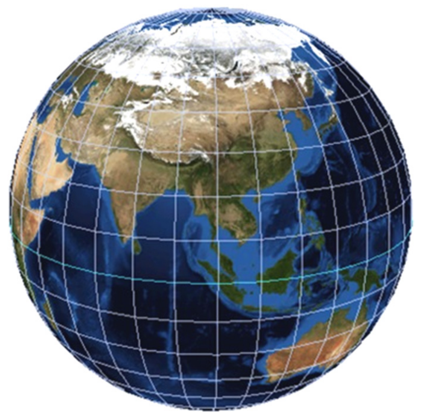
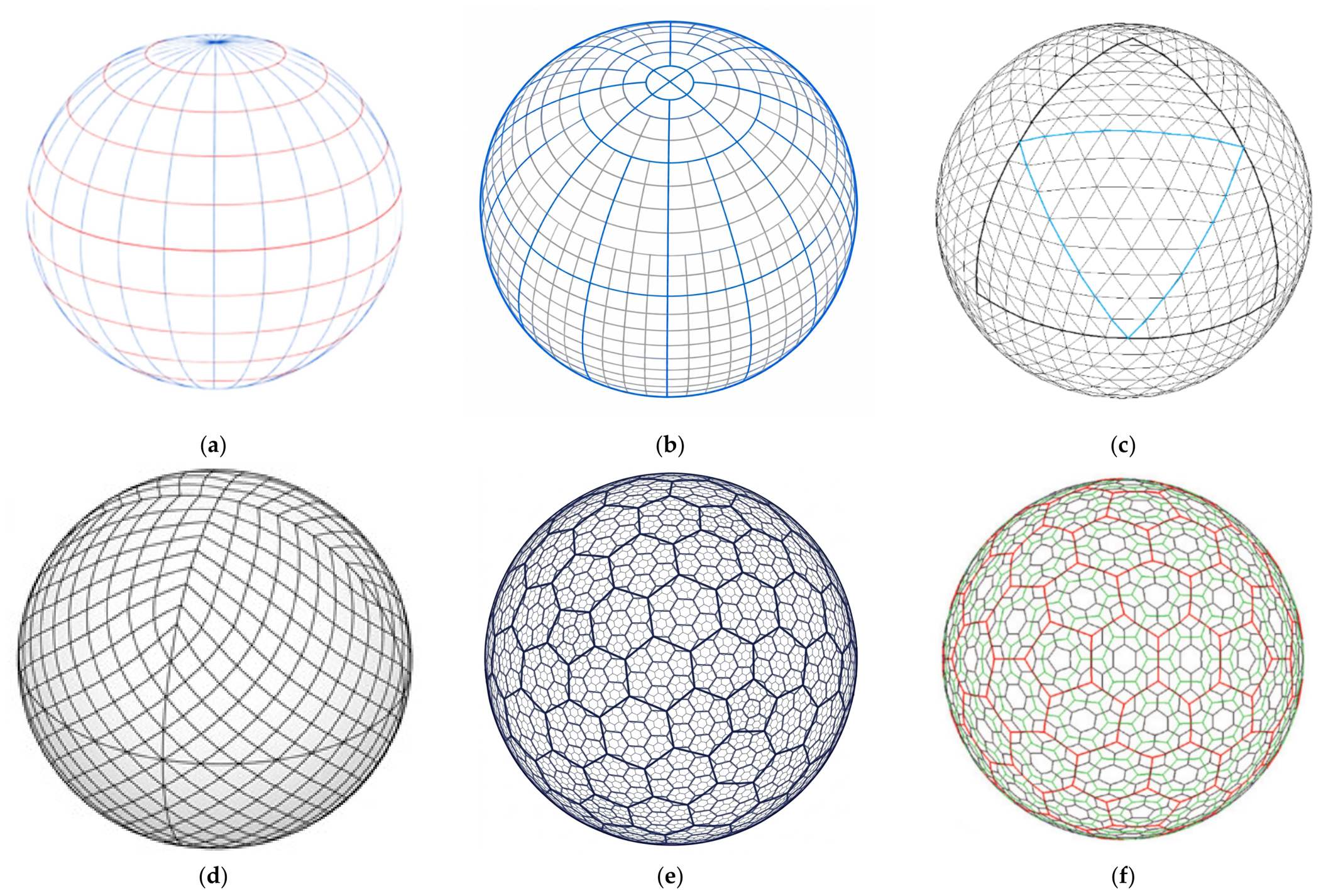
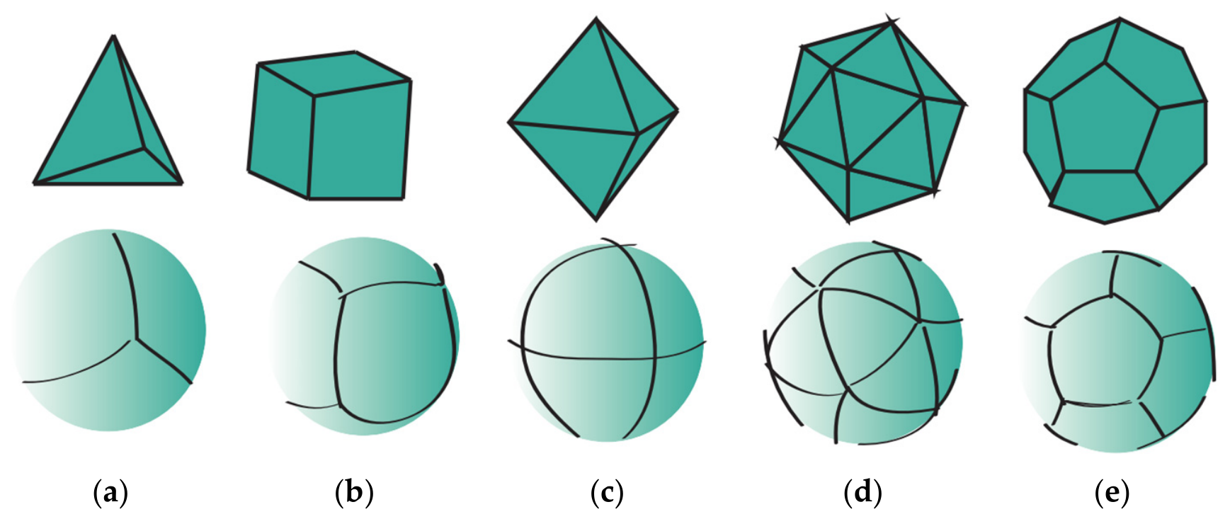
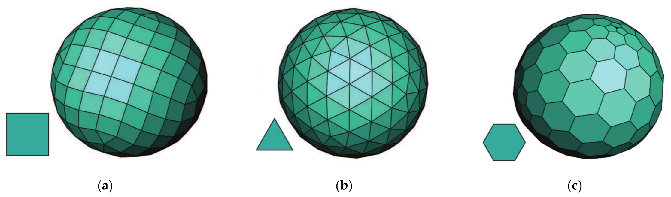
DGGS are a global regional location reference system that recursively partitions the Earth’s space using specific subdivision methods to form a seamless, non-overlapping, multi-scale discrete grid structure. Its development has broadly evolved from latitude–longitude grids, to regular polyhedral spherical grids, and finally to standardized Discrete Global Grid Systems. Early digital Earth platforms, such as Google Earth and NASA World Wind, primarily used latitude–longitude grids to organize global imagery and terrain data. However, such grids suffer from polar convergence, area distortion, and scale imbalance in high-latitude regions. From the 1980s to the 1990s, researchers began to shift toward regular polyhedral spherical tessellations. Dutton proposed the Quaternary Triangular Mesh (QTM) [8], while Goodchild and colleagues introduced the Hierarchical Spatial Data Structure (HSDS) [9], both enabling global multi-resolution representation through recursive triangular subdivision. Since the beginning of the 21st century, models such as HTM [10], HEALPix [11], and ISEA3H [12] have been developed successively, with an emphasis on balancing area preservation and adjacency consistency. With the growth of internet-based location services and large-scale spatiotemporal data analytics, engineering-oriented DGGS such as Google S2 [13] and Uber H3 [14] have been widely adopted. The former constructs a global hierarchical quadrilateral grid based on cube projection, whereas the latter employs an icosahedral hexagonal grid system to support urban computing, mobility analysis, and spatial aggregation. In China, GeoSOT [15] extends the global latitude–longitude space into a 2ⁿ-based regular subdivision system, enabling unified encoding and efficient retrieval of remote sensing imagery, real-estate units, and massive spatial datasets [16]. A series of studies based on octahedral grids [17], icosahedral grids [18], rhombic grids, composite rhombic grids [19], and rhombic triacontahedra [20] have further enriched the subdivision forms, encoding methods, and application scenarios of spherical DGGS. Overall, two-dimensional spherical DGGS have gradually evolved from an early geometric tessellation model oriented toward cartographic representation and visualization into a fundamental infrastructure supporting global spatial indexing, multi-scale analysis, and high-performance computing.

With the development of Earth system science, digital twin Earth, and integrated space–air–ground–sea observation, the limitations of two-dimensional DGGS have become increasingly evident in volumetric representation, radial subdivision, cross-sphere topological relationships, and three-dimensional physical-field computation. Accordingly, introducing a radial dimension into DGGS to construct an Earth System Spatial Grid (ESSG), also referred to as a 3D-DGGS, has become a critical research frontier in the evolution of global spatial information frameworks. Early three-dimensional extensions were mainly developed for seismic tomography and mantle dynamics simulation [21]. Between 2009 and 2012, Wu, Yu, and colleagues proposed the Spheroid Degenerated Octree Grid (SDOG) and applied it to multi-scale three-dimensional modeling and visualization of the global lithosphere [22,23], promoting the extension of DGGS from spherical surface cells to volumetric Earth cells. Around 2013, models such as S³G [24] and SGOG [25] explored three-dimensional digital Earth spatial frameworks from the perspectives of layered spherical organization and radial extension based on regular polyhedra, respectively. After 2015, GeoSOT-3D improved the organization and retrieval efficiency of massive 3D spatial data through three-dimensional integer encoding [26].

From 2018 to 2020, studies on GHOST [27] and general methods for 3D-DGGS extension [28] further emphasized equal-volume mapping, radial subdivision, and voxel morphology control. These developments indicate that ESSG has moved beyond simple three-dimensional geometric tessellation toward the construction of volumetric grids designed for spatial computation and numerical simulation. In recent years, models such as ISEA4H-ESSG [29] and SGDOG [30] have continued to investigate multi-layer spatial representation, radially degenerated subdivision, and cross-sphere encoding, further enhancing the adaptability of ESSG to complex Earth system processes.

ESSG is expected to become a standardized spatial foundation for the integrated representation and simulation of the atmosphere, oceans, underground space, lithosphere, and near-Earth space. In 2020, the Open Geospatial Consortium (OGC) issued a public call for comments on Version 2.0 of the DGGS standard [31], with the proposed inclusion of three-dimensional equal-volume grids. This marks a shift in the research focus of Earth System Spatial Grid from early “geometric grid drawing” toward the construction of a “high-performance three-dimensional spatial computing engine.” The aim is to provide a standardized and highly interoperable three-dimensional grid algebra foundation for complex fluid and solid entities across multiple Earth spheres, including the atmosphere, hydrosphere, and lithosphere.

Several high-quality reviews have documented the evolution of DGGS from different perspectives. Mahdavi-Amiri et al. [1] provided a mathematical survey of Digital Earth frameworks with a focus on indexing methods and conversions. Zhao et al. [19] systematically summarized the modeling, encoding, and quality evaluation of terrestrial grids. In the context of big data, Yao et al. [32] explored the synergy between cloud computing and DGGS for Earth observation. Most recently, Su et al. [33] established a systematic framework linking grid subdivision, encoding, and storage to reveal their collaborative potential. However, no existing review has provided a unified and comparative analysis of the geometric construction, radial extension mechanisms, encoding methods, and application paradigms of the full spectrum of Earth System Spatial Grid, spanning shell-based, volumetric, and unstructured approaches. This paper aims to fill this gap by providing a multidimensional classification framework that distinguishes the primary design intent of a grid from its geometry, hierarchy, indexing capability, cross-layer topology, and numerical-discretization role, and by using this framework to comparatively evaluate representative ESSG and to identify critical challenges for future development.

To trace the technical evolution of Earth System Spatial Grid, this paper first reviews their two-dimensional foundation, namely spherical Discrete Global Grid Systems (DGGS). It then examines the construction methods of Earth System Spatial Grid along four technical routes: latitude–longitude spherical grids, regular polyhedral grids, finite-element unstructured grids, and voxel-based tessellations. On this basis, the paper comparatively analyzes key technical indicators of different grid types, provides a comprehensive overview of their encoding methods and application paradigms, and finally presents a systematic outlook on frontier challenges.

This paper is organized as a structured narrative review, aimed at synthesizing and comparatively analyzing the conceptual evolution and technical characteristics of representative Earth System Spatial Grid (ESSG) models. We describe the methodology as a structured narrative review because, although the literature search follows an explicit and documented strategy (detailed below), the final selection relies on expert judgement and does not implement the complete screening workflow required of a fully systematic review. To ensure the transparency and reproducibility of the literature-selection process, the relevant publications were identified through Web of Science, Scopus, IEEE Xplore, and Google Scholar, supplemented by targeted searches of leading venues in the field (e.g., ISPRS International Journal of Geo-Information, International Journal of Geographical Information Science, and Acta Geodaetica et Cartographica Sinica) and by the technical documentation and open-source repositories of engineering-oriented systems (e.g., the OGC Abstract Specification, S2, H3, and DGGRID). The search combined the following keyword groups: (“discrete global grid systems” OR “DGGS” OR “geodesic grid” OR “global grid”) AND (“three-dimensional” OR “3D” OR “volumetric” OR “voxel” OR “radial” OR “Earth System Spatial Grid” OR “ESSG”), together with model-specific names such as SDOG, SGOG, HEALPix, GeoSOT, ISEA, MPAS, and Yin-Yang. The search covered publications from the 1980s—when foundational work on polyhedral and geodesic global grids began—to September 2026; seminal early studies were deliberately retained to preserve the conceptual lineage of the field, while particular attention was paid to work from the last five years to ensure adequate coverage of recent advances. A study was included if it (i) proposed, extended, or evaluated a global (spherical or ellipsoidal) discrete grid with an explicit two- or three-dimensional partitioning mechanism, (ii) addressed encoding, indexing, or topological methods for such grids, or (iii) reported a representative application of such grids in Earth system science; a study was excluded if it concerned only local or planar grids without a global reference frame, employed grids merely incidentally without a methodological contribution, or was unavailable in English or Chinese. For each of the four technical routes, representative models were selected on the basis of originality, citation impact, methodological completeness, and continued influence on subsequent work, so that the surveyed set reflects both the historical foundations and the current state of the art rather than an exhaustive enumeration of every published variant. As is inherent to a structured narrative review, the final selection involves a degree of expert judgement rather than a fully reproducible systematic-review screening protocol; the aim is to capture the principal technical routes and their evolution rather than to catalogue all existing implementations.

2. Discrete Global Grid Systems

Discrete Global Grid Systems can be classified, according to their spherical base, into latitude–longitude grids and polyhedral grids. To visually illustrate the differences among representative DGGS in terms of base polyhedron, cell morphology, and subdivision structure, Figure 1 presents schematic examples of several typical spherical DGGS and their grid-cell forms.

2.1. Latitude–Longitude Grids

In latitude–longitude grids, cell boundaries are generally formed by orthogonal meridians and parallels, as shown in Figure 2. Owing to their natural compatibility with geographic coordinate systems, such grids were widely used in early digital Earth platforms, including Google Earth and NASA World Wind, for organizing image pyramids and enabling rapid visualization of terrain data. Cheng Chengqi of Peking University improved this type of grid by proposing GeoSOT (Geographic Coordinate Subdividing Grid with One-Dimension Integral Coding on 2ⁿ Tree) [15]. GeoSOT extends the global geographic domain to 512° × 512°, thereby enabling efficient spatial coordinate retrieval at the bit-operation level. It has been applied to remote sensing image management [16] and real-estate unit coding and identification [36].

However, latitude–longitude grids degenerate rapidly from the equator toward the poles. This not only causes substantial data redundancy in high-latitude regions, but also leads to severe cell deformation. To address this issue, Cui Majun et al. [37] proposed a degeneration-based subdivision strategy to alleviate grid-cell convergence in high-latitude regions, namely the Degenerate Quad-tree Grid (DQG). This method attempts to mitigate polar convergence by merging cells near the polar regions. Nevertheless, the resulting inconsistency in topological structure introduces additional computational burdens for cross-regional spatial relationship reasoning.

2.2. Polyhedral Grids

Polyhedral grids are characterized by cell boundaries that are generally formed by geodesic lines. Most existing Discrete Global Grid Systems are constructed on spherical grids derived from the five regular polyhedra, namely the tetrahedron, cube, octahedron, dodecahedron, and icosahedron, as shown in Figure 3. By projecting polyhedral faces onto the sphere along great-circle arcs, these models form approximately uniform hierarchical grid structures. The resulting cell shapes mainly include triangles, quadrilaterals, and hexagons, as shown in Figure 4.

Triangular cells are fundamental geometric primitives and are advantageous for rendering, but their adjacency relationships are variable and relatively complex. Representative examples include the Quaternary Triangular Mesh (QTM) [38] proposed by Dutton [8], the Hierarchical Spatial Data Structure (HSDS) proposed by Goodchild [9], and the Hierarchical Triangular Mesh (HTM) proposed by Kunszt [10]. To reduce geometric distortion, subsequent studies have shifted toward base polyhedra with a larger number of faces or more sophisticated projection methods. Lin Bingxian et al. [39] investigated encoding methods based on the icosahedron for ocean dynamics modeling. Hall et al. [40] constructed a triangular grid system on the hecatonicosahedron, while Wang Rui et al. [41] developed a triangular grid system on the surface of the rhombic triacontahedron, thereby improving the efficiency of grid construction.

Quadrilateral grids are similar to conventional square pixel-based data structures, allowing many existing algorithms to be directly transferred. However, they do not ensure uniform adjacency. Bai et al. [17] and Zhou et al. [18] constructed hierarchical rhombic grids based on the octahedron and icosahedron, respectively. Subsequently, Zhao et al. [19] proposed a composite rhombic grid structure and released the open-source project OpenDGGS, which supports grid generation for systems with multiple cell shapes. In terms of applications, Lamberts et al. developed the Ellipsoidal Cube Map (ECM) for visualizing planetary surface topography, while Google S2 [13] established a global quadrilateral grid system. HEALPix [11], based on the rhombic dodecahedron, and SCENZ-Grid (Solid Earth and Environment GRID) have been adopted by NASA for astronomical data analysis and global environmental monitoring.

Hexagonal grids provide uniform adjacency and offer the highest sampling efficiency and angular resolution. However, they lack self-similarity and tend to produce relatively complex fractal subdivision structures. Sahr et al. [42] investigated the Icosahedral Snyder Equal Area Aperture 3 Hexagon grid (ISEA3H), which is based on the Snyder projection [12], and released the grid generation software DGGRID version 6.2 [43]. Uber developed the global discrete grid system H3 [14] for indexing large-scale ride-hailing data. Bush developed the grid toolkit OpenEAGGR version1.0.1 [44], which supports triangular and hexagonal coding and indexing and provides spatial analysis functions. Very recently, Kmoch et al. [45] introduced IGEO7, an open-source aperture-7 hexagonal equal-area DGGS with the hierarchical Z7 integer indexing system implemented in DGGRID; IGEO7 provides strictly equal-area cells, combining H3-style hierarchical indexing with the area fidelity required for sound statistical analysis. Liang Xiaoyu et al. [20] proposed a method for constructing a hexagonal Discrete Global Grid based on the rhombic triacontahedron, which offers the advantage of reduced geometric distortion. More recently, Wecker et al. [46] generalized this construction philosophy by adopting high-resolution spherical meshes, rather than Platonic or Catalan solids, as the base polyhedra of a DGGS, thereby significantly reducing areal and angular distortion while retaining constant-time hierarchical indexing operations.

The development of the above spherical DGGS has provided a geometric foundation and standardized framework for ESSG. Nevertheless, extending a two-dimensional spherical grid to a three-dimensional spherical volume is not a simple matter of adding one more dimension. Rather, it requires a systematic reconstruction involving radial mapping, volume preservation, and topological consistency.

3. Earth System Spatial Grid (ESSG)

3.1. Definition of ESSG

The Earth System Spatial Grid (ESSG) is a named concept with an identifiable lineage rather than a term coined in the present review. It was introduced by Wu Lixin and colleagues, who argued that a universal spheroidal Global Spatial Grid oriented to the Earth system should be treated as a distinct class of grid, and it was subsequently positioned within the Group on Earth Observations (GEO) framework as a Global Spatial Reference Frame for the distribution, sharing, and interrelation of global datasets across the Earth’s spheres [47]. Formally, an ESSG mathematically abstracts the entire volumetric Earth space into an Earth-system space and, following a deterministic subdivision rule, discretizes it into a hierarchy of cells each carrying a unique identifier; its concrete realization is fixed by three components—a reference spheroid, a subdivision scheme, and an encoding system. Conceptually it occupies the three-dimensional (spheroidal) branch of the global-spatial-grid taxonomy: whereas DGGS tessellate a two-dimensional spherical manifold, the ESSG extends such a tessellation into the radial dimension so as to fill the volumetric Earth space.

In the wider literature, systems of this class are also described more neutrally as three-dimensional DGGS (3D-DGGS). The two are best understood as near-synonymous designations of the same class of system that differ in emphasis rather than in substance: “3D-DGGS” foregrounds the technical mechanism of extending a two-dimensional DGGS along the radial direction, whereas “ESSG” foregrounds the system-level goal of representing the atmosphere, hydrosphere, lithosphere, and near-Earth space as a coupled whole.

An ESSG is more than “a DGGS with an extra radial axis”. The following seven properties define an ideal reference-indexing ESSG (design intent A); they specify what a grid should achieve when its primary purpose is to serve as a stable, reproducible global spatial reference:

(1)

Volumetric coverage. At every resolution level the cells must fill the entire three-dimensional Earth space—from the deep interior through the surface to near-Earth space—seamlessly and without gaps or overlaps, so that each point belongs to exactly one cell.

(2)

Hierarchical, multi-resolution structure. The system must comprise grids of successively finer resolution generated by a recursive subdivision rule, ideally supporting asynchronous refinement in the radial and tangential directions to accommodate the strongly anisotropic sampling of Earth-system data.

(3)

Well-defined parent–child and neighbourhood relations. The subdivision must induce a deterministic parent–child hierarchy together with unambiguous adjacency relations among cells at a given level, so that hierarchical aggregation/disaggregation and neighbourhood queries can be resolved directly and consistently.

(4)

Approximate size uniformity. Cells at the same level should have comparable—ideally near-equal—volumes, or maintain a controlled ratio between radial and tangential edge lengths, so as to avoid the severe centripetal distortion in which cells shrink toward the geocentre.

(5)

Geographic consistency. Cells must be defined with respect to a formally declared geodetic reference system (datum and coordinate reference system), such that the mapping between cells and geographic coordinates is rigorous and invertible.

(6)

Unique and efficient cell addressing. Every cell must carry a globally unique, stable identifier encoding both its level and position, supporting efficient forward/inverse conversion and spatial indexing, and, where required, extension to a spatiotemporal identifier.

(7)

Multi-source data compatibility. As a system-level attribute, the ESSG should serve as a common reference frame integrating heterogeneous multi-source data of differing formats, resolutions, and semantics, enabling seamless interoperability and cross-layer analysis.

These seven properties constitute an idealized target for reference-indexing frameworks rather than a checklist that any single model fully meets. Importantly, they should not be applied uniformly to grids whose primary intent is numerical discretization: for such grids—Spiral Grid, SCVT, and MPAS being typical examples, and their absence reflects a different purpose rather than a deficiency. The appropriate criteria for intent-B grids are instead numerical, including conservation, anisotropic adaptivity, and solver stability.

The seven properties above make clear that not every grid discussed under the ESSG umbrella is designed for the same purpose, and a single-axis taxonomy is therefore insufficient. To avoid conflating systems of different conceptual nature, we organize the following review around a multidimensional classification that separates what a grid is designed for from how its three-dimensional cells are geometrically generated.

At the top level, we distinguish two primary design intents. (A) Reference and indexing frameworks treat the grid first and foremost as a global spatial reference: their defining requirement is a stable, reproducible cell identity together with an invertible spatial addressing scheme, so that the same cell is assigned the same code across time, platforms, and datasets. (B) Numerical discretization meshes treat the grid first and foremost as a substrate for solving partial differential equations: their defining requirement is numerical accuracy and stability, and to attain it they may be dynamically refined, adaptively coarsened, or repartitioned, so that a cell has no obligation to carry a persistent global identifier. This distinction is essential for interpreting models such as Yin–Yang, SCVT, and MPAS, which are highly successful as numerical meshes but were never intended to serve as reproducible spatial-indexing systems. We further observe that these two lineages are beginning to converge: a small number of models originally rooted in the numerical-mesh tradition have been equipped with standardized encoding interfaces, ISEA4H-ESSG being the representative case. Rather than introducing a separate third class for such single-instance cases, we mark this transition through a primary-intent attribute in the comparison matrix of Section 3.5.

At the second level, which also provides the organizing axis for the subsections below, models are grouped by their geometric construction strategy—that is, by how the three-dimensional cell is generated: shell-based grids stack two-dimensional spherical tessellations along the radial direction; volumetric grids subdivide the solid ball directly and treat the geocentric singularity as an explicit design object; and unstructured grids generate cells from Voronoi/Delaunay constructions without a fixed hierarchical rule. We stress that this geometric axis is not fully orthogonal—shell-based grids can carry volumetric cells, and unstructured meshes can be organized into multiple spherical layers—which is precisely why the geometric grouping alone cannot fully characterize a model. To resolve this ambiguity, each model is additionally described in Section 3.5 along six independent dimensions: geometry, hierarchy, indexing capability, cross-layer topology, numerical-discretization role, and primary design intent.

3.2. Shell-Based Grids

3.2.1. Latitude–Longitude Spherical Grid Methods

The most direct approach to extending DGGS along the radial dimension is to inherit the orthogonal partitioning of the geographic coordinate system, yielding what is commonly called the three-dimensional latitude–longitude grid system (3D-LLGS). This scheme treats (λ, φ, r) as three independent axes, each recursively subdivided. Because such a partition is topologically isomorphic to a regular three-dimensional array, it can be directly consumed by conventional GIS engines and by finite-difference stencils. Early whole-mantle P-wave tomography inversions exploited exactly this property to embed observational travel-time residuals into a global voxel framework [21].

The principal engineering weakness of 3D-LLGS is not its geometry but its data-access cost: floating-point coordinates must be repeatedly transformed into cell indices, and the resulting indices are difficult to align across resolution levels. GeoSOT-3D was designed to remove this bottleneck rather than to alter the underlying spherical geometry [26]. By embedding the physical Earth into a normalized 512° × 512° × 512° virtual cube and encoding each axis with a 2ⁿ-tree, GeoSOT-3D reduces spatial queries to integer bit operations by construction, with the advantage of reducing in query cost attributable to the elimination of floating-point-to-index transformation [48]. Yet, because the underlying partition is still meridian-parallel, the intrinsic polar convergence and the geometric collapse toward the Earth’s center persist and, at the highest subdivision levels, manifest as computational singularities.

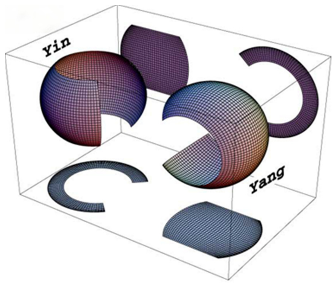
A different route is to circumvent the polar problem geometrically. Kageyama and Sato’s Yin-Yang grid [49] tiles the sphere with two mutually orthogonal low-latitude patches, so that each patch inherits only the well-behaved equatorial portion of a latitude–longitude mesh, as shown in Figure 5. The design has proven effective in mantle convection, numerical weather prediction [50], and global MHD simulation [51], but the overlap zone between the two components incurs redundant storage and demands interpolation whenever fluxes or fields must be exchanged. It should be noted that, although the Yin–Yang grid is geometrically a latitude–longitude construction and is therefore discussed here alongside GeoSOT-3D and S³G, its primary design intent differs fundamentally: as an overset mesh it does not maintain a stable, globally unique cell identity, and it is accordingly classified as a numerical-discretization grid (intent B) rather than a reference-indexing framework (intent A) in the taxonomy of Section 3.5. A complementary layered strategy is proposed by S³G [24], which decouples the vertical structure of the Earth system into independent spherical shells, each carrying its own two-dimensional grid. Such modularity is attractive for multi-sphere data management, but it defers rather than solves the problem of cross-layer topological continuity.

3.2.2. Regular-Polyhedron-Based Spherical Grid Methods

1.

Extensions Based on the Octahedron/QTM

Among polyhedral extensions, the octahedron and the icosahedron have been the dominant base solids. The SGOG model [25] takes the spherical QTM as its horizontal skeleton and stacks its triangular cells radially through an octree-like organization, producing prism-shaped voxels that inherit QTM’s clear hierarchical indexing while offering a first realization of true 3D tiling for Digital Earth. The unavoidable side effect of such uniform radial stacking is that voxels near the Earth’s center become geometrically ill-conditioned: their aspect ratios diverge and their volumes shrink toward zero [52].

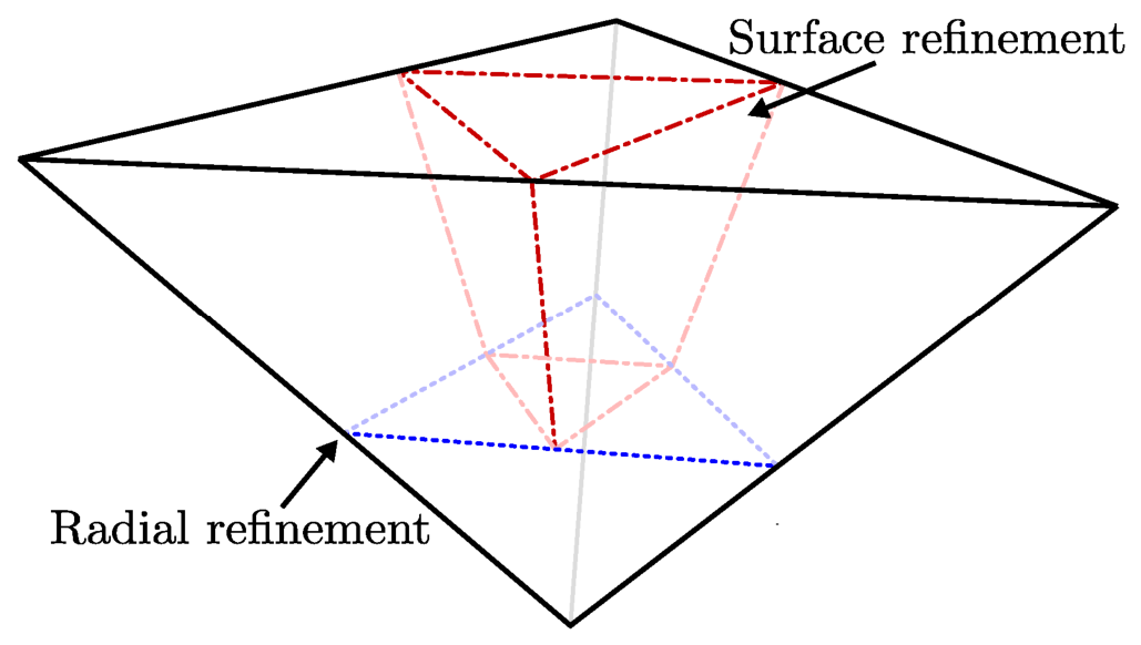
SGDOG [30] addresses this by introducing depth-dependent QTM refinement (Figure 6): the horizontal level is progressively coarsened as the radius decreases, so that voxel volume distortion is bounded rather than allowed to grow with depth. The horizontal level and the radial level are then fused into a single hierarchical identifier, which preserves QTM’s parent–child arithmetic while accommodating heterogeneous vertical resolutions. Beyond its immediate use for volumetric modeling, SGDOG demonstrates a general design principle: for polyhedral 3D-DGGS, radial adaptivity should be governed by an explicit, computable distortion budget rather than by a fixed stacking rule.

2.

Extensions Based on the Icosahedron

The icosahedron provides a closer initial approximation of the sphere than the octahedron, and its Snyder equal-area projection yields spherical cells whose areas differ only marginally. These properties make it a natural base for fluid-oriented Earth-system grids. Early icosahedral 3D extensions were essentially numerical-analysis constructs—e.g., Baumgardner’s uniform radial replication of triangular layers for mantle-flow discretization [53] and were not intended to serve as indexable data infrastructures. Subsequent work moved toward geophysically informed radial partitions, exemplified by Ballard et al. [54], who constrained radial nodes to lie on true Earth discontinuities such as the Moho and the CMB.

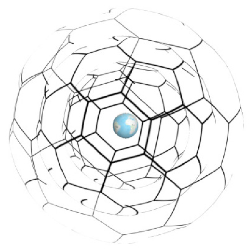
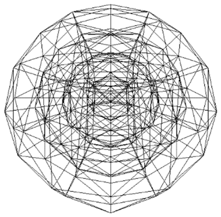
The ISEA4H-ESSG model of Ma et al. [29] (Figure 7) marks the transition from numerical-tool status to a full ESSG: an aperture-4 hexagonal spherical grid is coupled with a radial degeneration mechanism that adaptively coarsens deep cells, so that volume disparity between the atmospheric shell and the deep interior is contained. Crucially, the model exposes an encoding interface amenable to standardized 3D indexing, which distinguishes it from its numerical-simulation predecessors. The remaining open problem for icosahedral 3D-DGGS is algebraic rather than geometric: the lack of an orthogonal radial partition makes cross-level neighbor arithmetic considerably more expensive than in octahedron-based schemes, and a lightweight algebraic mapping theory is still needed to support massive-scale parallel access.

3.

Three-Dimensional Polyhedral Mapping and General Extension Theory

Research on the three-dimensional extension of polyhedral grids has gradually shifted from early geometric construction toward isomorphic mapping between complex manifolds and the preservation of key geometric properties. In 2018, Holhoş and Roşca [55] made an important mathematical contribution by constructing a series of equal-volume mapping functions from the cube to the tetrahedron, octahedron, and sphere. These mappings addressed the stability of polyhedral cells during refinement and provided a solid foundation for multi-resolution representation in three-dimensional grids. In the same year, Thieulot [27] developed the GHOST framework based on the concept of a “geological hollow sphere” and further examined the influence of conformal and equidistant projections on volumetric consistency. The results demonstrated that, in solid Earth simulations, conformal projections provide higher numerical accuracy in maintaining the topological coupling between radial layers and spherical surface grids. Ulmer et al. [28] proposed a general extension paradigm for 3D-DGGS, as shown in Figure 8. This theory moves beyond the constraints of specific geometric solids by decomposing the construction of a 3D-DGGS into two components: a spherical base grid and a radial mapping. By introducing radial mapping functions, the method enables a dynamic balance between volume preservation and shape compactness. As a result, three-dimensional extension no longer merely pursues geometric symmetry. Instead, through dimensional decoupling and radial mapping parameterization, it achieves logical consistency between two-dimensional spherical indexing and three-dimensional volumetric indexing. This general extension theory not only mitigates polar distortion and radial degeneration, but also allows fine control of cell aspect ratios. Consequently, the resulting grids can flexibly meet multi-scale application requirements, ranging from large-scale satellite orbit tracking to micro-scale urban building modeling.

3.3. Volumetric Grids

Unlike shell-based schemes, which regard the sphere as a stack of two-dimensional grids, volumetric approaches partition the ball itself and treat the geometric singularity at the Earth’s center as an explicit design object rather than a defect to be avoided. The Spheroid Degenerated Octree Grid (SDOG), introduced by Wu and Yu in the context of the 3DGES framework [22,23], is the canonical realization of this idea. Standard octree subdivision would produce eight isotropic children per parent cell, but on a sphere such uniformity is incompatible with the geodetic coordinate system near the poles and the geocenter. SDOG resolves this incompatibility by explicitly introducing degenerated subdivisions—cells that split into four or two children rather than eight—thereby preserving a well-defined parent–child topology throughout the entire ball.

Two subsequent developments consolidated SDOG’s position as a computation-oriented framework rather than merely a discretization scheme. The geometry–topology–attribute ternary model of Yu et al. [56] made SDOG usable as a data organization layer for large-scale, cross-layer geological bodies, avoiding the fragmentation typical of Euclidean-embedded 3D geology. Ulmer and Samavati [57] subsequently equipped SDOG with non-stationary subdivision rules and adaptive offset surfaces, which enforce an approximate global equal-volume property outside the degeneration cores. The combination of geodetic compatibility, controlled singularity, and explicit topology has made SDOG a reference model against which other volumetric schemes are typically compared. In terms of design intent, SDOG is a reference-indexing framework (intent A): its degenerated octree induces a deterministic parent–child hierarchy and a globally unique, decodable cell identity, which is what allows it to serve as a data-organization layer rather than merely a discretization scheme, even though it is also employed in numerical applications such as tomographic parameterization.

3.4. Unstructured Grids

When neither radial stacking of a regular polyhedron nor octree-style volumetric refinement can accommodate the anisotropy of a target physical process, unstructured spherical grids become attractive. The essential trade-off is well known: relaxing hierarchical regularity buys geometric flexibility at the cost of implicit topology and irregular memory access. In terms of the present taxonomy, the models discussed in this subsection are predominantly numerical-discretization grids (intent B): they are included not because they provide indexing capabilities equivalent to a DGGS, but because their geometric construction and their sustained influence on Earth-system practice make them an indispensable part of the technical lineage. Their cells are typically generated to satisfy numerical criteria and may be adaptively refined or repartitioned, so that a persistent global cell identity is generally absent.

The Spiral Grid of Hüttig and Stemmer [58] exemplifies the “geometric flexibility” end of this spectrum. Nodes are seeded along a Fibonacci-type spiral on each spherical shell, and their natural-neighbor Voronoi diagram defines the cells; radial layers can be added or refined independently, yielding nearly volume-uniform cells across the entire mantle even under strong local refinement. Independently, Ringler et al. [59] introduced spherical centroidal Voronoi tessellations (SCVT) into climate modeling and equipped them with user-controlled density functions, which allowed key regions—ice-sheet margins, ocean eddies, coastal boundaries—to be resolved without abrupt resolution jumps. The subsequent MPAS framework [60] integrated SCVT with C-grid staggering, so that global climate simulation and regional high-resolution NWP could share a single grid substrate.

These successes have positioned unstructured schemes as the default choice for adaptive Earth-system simulation. Their principal limitations are architectural rather than geometric: neighbor lists must be stored explicitly, memory access is indirect, and domain decomposition for parallel execution is significantly harder than for hierarchical grids. Consequently, an active line of research is to reconcile Voronoi-style adaptivity with the deterministic hierarchical encoding of standardized DGGS, so that adaptive cells can be addressed and exchanged through a common algebra.

This line of work can be read as an attempt to move unstructured meshes from intent B toward intent A, and it mirrors, from the opposite direction, the convergence already observed for encoding-enabled icosahedral models such as ISEA4H-ESSG.

3.5. Comparative Analysis of Representative ESSG Models

To operationalize the multidimensional classification introduced in Section 3.1 and to make the differing roles of the reviewed models explicit,

Table 1. Multidimensional classification of representative Earth System Spatial Grid models.

Model	Design Intent	Geometry (Basis)	Hierarchy Type	Indexing Capability	Cross-Layer Topology	Numerical Discretization Role
3D-LLGS	A	Latitude–longitude	Recursive	Coordinate-derived	Consistent	Compatible with FD stencils
GeoSOT-3D	A	Latitude–longitude	Recursive 2n-tree	Global code	Consistent	Indexing only
Yin–Yang	B	Latitude–longitude	Layer- independent	None	Weak	PDE-oriented
S3G	A	Layered spherical shells	Layer- independent	Global code	Weak	Indexing only
SGOG	A	Octahedron/QTM	Recursive octree	Global code	Moderate	Indexing-oriented
SGDOG	A	Octahedron/QTM	depth-adaptive	Global code	Moderate	Indexing-oriented
ISEA4H-ESSG	A	Icosahedron	radially degenerate	Global code	Relatively strong	Both
SDOG	A	Voxel ball	Recursive octree	Global code	Strong	Indexing + local numerical use
Spiral Grid	B	Unstructured	Non-hierarchical	None	Weak, implicit	PDE-oriented
MPAS (SCVT)	B	Unstructured (SCVT)	Non-hierarchical, adaptive	None	Weak	PDE-oriented

characterizes each representative model along six independent dimensions: primary design intent, geometric basis, hierarchy type, indexing capability, cross-layer topology, and numerical-discretization role. The matrix shows that models frequently grouped together by a single geometric label in fact occupy very different positions once these dimensions are separated. GeoSOT-3D and SDOG, for instance, are reference-indexing frameworks (intent A) defined by stable, decodable cell identities, whereas Yin–Yang and MPAS, though geometrically unrelated to each other, share the intent-B profile of numerical meshes without persistent global addressing. Read column-wise, the matrix confirms that latitude–longitude-based methods remain compatible with conventional GIS but retain polar and centripetal distortion; polyhedral methods improve hierarchical regularity at the cost of equal-volume and cross-layer topological guarantees; and volumetric and unstructured approaches offer the strongest support for physical-field simulation and adaptive modeling while demanding more complex encoding, storage, and computation.

Table 1 deliberately reports design characteristics rather than performance. To place the comparison on a reproducible footing,

Table 2. Quantitative geometric-quality indicators for representative ESSG models. The compactness column reports heterogeneous, non-commensurable indicators (three-dimensional sphericity Ψ, two-dimensional isoperimetric compactness C, and qualitative classes); the metric type is stated for each entry, and values based on different metrics should not be ranked directly against one another.

Model	Vmax/Vmin	Compactness (Metric Type)
3D-LLGS [21]	Divergent	Ψ → 0 (3D)
GeoSOT-3D [26]	Divergent	Low near poles (qualitative)
Yin–Yang [49]	Non-equal (poles solved, centre unsolved)	Moderate (qualitative)
S3G [24]	1.004 × 107 (converged)	Moderate (qualitative)
SGOG [25]	Area ratio → 2; volume divergent radially	Moderate (qualitative)
SGDOG [30]	8.43 (converged)	Moderate (qualitative)
ISEA4H-ESSG [29]	Bounded (radially degenerate)	C ≈ 0.907 (2D)
SDOG [22,23]	8.88	Ψ = 0.799 (3D)
Modified SDOG [22,23]	2.63	Ψ = 0.767 (3D)
Spiral Grid [58]	≈1.21	High (qualitative)
MPAS (SCVT) [60]	≈1 (density-controlled)	C ≈ 0.907 (2D)

supplements the classification with two geometric quality indicators for which the literature or a closed-form derivation provides explicit values. It is important to stress that these indicators are not mutually commensurable and should not be read as a single homogeneous compactness measure: three-dimensional cell compactness is expressed by the sphericity Ψ (the surface-area ratio between a volume-equivalent sphere and the cell; Ψ = 1 for a perfect sphere), whereas two-dimensional surface-cell compactness is expressed by the isoperimetric ratio C = 4πA/P² (C = 1 for a circle, with the regular-hexagon bound at 0.907); these are quantities of different dimensional and geometric character, and the volume ratio V_max/V_min is a third, distinct descriptor. To make this explicit, Table 2 states the metric type for each entry, and no cross-metric ranking is implied between rows characterized by different indicators.

Where a single number is not meaningful, we report qualitative ratings. The thresholds used for these ratings are operational heuristics adopted in this review for descriptive convenience rather than generally established standards. Under this convention, equal-volume behaviour is rated near-equal when V_max/V_min converges to a bounded constant below 10, and non-equal/divergent when V_max/V_min grows without bound as the level increases; compactness is rated high when the corresponding measure remains high and bounded (Ψ ≥ 0.8, or C approaching the regular-hexagon bound 0.907), moderate when it decreases but stays bounded, and low when cells degenerate toward the poles or the geocentre. These thresholds are heuristic and are intended only to summarize the source-reported values in a consistent vocabulary, not to impose an absolute quality standard.

Table 1 and Table 2 support application-driven selection rather than a single ranking. When reproducible identity and cross-dataset interoperability dominate—as in data cataloguing, multi-source fusion, and archiving—frameworks with closed-form indexing and bounded volume ratio are preferable; among these, the volume-preserving SDOG variant is a representative choice that combines exact addressing with controlled volume variation. When numerical fidelity dominates—as in mantle-convection or coupled climate simulation—compact, quasi-uniform meshes such as the Spiral Grid and SCVT/MPAS are better suited, at the cost of relying on stored adjacency and lacking a persistent global code. Latitude–longitude-inheriting grids (3D-LLGS, GeoSOT-3D) remain the most interoperable with conventional GIS but exhibit divergent volume ratios toward the poles and geocentre, whereas hexagonal (ISEA4H-ESSG) and great-circle-arc QTM grids (SGDOG) trade indexing simplicity against distortion in different ways. The mechanisms behind these radial ratios are analyzed in Section 3.6, and the encoding-level costs that accompany them in Section 4.3.

These geometric and topological differences directly determine the design of ESSG encoding mechanisms. Therefore, the Section 4 further reviews representative encoding methods for Earth System Spatial Grid.

3.6. Volumetric Geometry and Degeneration Control of Radial Subdivision

Extending a surface DGGS into three dimensions is not equivalent to appending an independent radial axis, because the volume of a three-dimensional cell is governed jointly by the solid angle Ω subtended by its surface cell and by the cubic difference in its inner and outer radial boundaries. For a cell bounded by r_in and r_out, the volume is $V=\left(\Omega /3\right)\left({r_{\mathrm{out}}}^3-{r_{\mathrm{in}}}^3\right)$.

This single relationship explains why the four polyhedral and volumetric families reviewed above adopt fundamentally different radial strategies. If the surface tessellation is (approximately) equal-area, Ω is nearly constant across cells at a given level, so the volume of a cell is controlled entirely by $\left({r_{\mathrm{out}}}^3-{r_{\mathrm{in}}}^3\right)$. Consequently, uniform radial spacing does not yield equal-volume cells: for a constant radial increment Δr, the volume of shells decreases rapidly toward the geocentre, and the radial-to-tangential aspect ratio degrades severely as r → 0, since the tangential edge length scales with r while Δr remains fixed.

The four representative models manage this cubic degeneration in distinct ways. SGOG stacks QTM triangular cells with a fixed radial rule; because both the tangential extent and the shell thickness shrink toward the centre without compensation, its inner voxels exhibit diverging aspect ratios and volumes approaching zero. SGDOG introduces depth-dependent coarsening of the horizontal QTM level, so that as r decreases the solid angle Ω is enlarged to partially offset the shrinking $\left({r_{\mathrm{out}}}^3-{r_{\mathrm{in}}}^3\right)$ term, bounding volume distortion rather than letting it grow monotonically with depth. ISEA4H-ESSG applies an analogous radial-degeneration mechanism on an aperture-4 hexagonal base, adaptively coarsening deep cells so that the volume disparity between the thin outer atmospheric shell and the deep interior is contained. SDOG attacks the singularity most directly at the volumetric level: rather than avoiding the geocentric degeneration, it makes it an explicit design object through degenerated subdivisions, and subsequent non-stationary subdivision rules with adaptive offset surfaces enforce an approximate global equal-volume property outside the degeneration cores. In summary, the appropriate way to compare radial-subdivision strategies is not by radial spacing alone but by how each controls the coupled behaviour of Ω and $\left({r_{\mathrm{out}}}^3-{r_{\mathrm{in}}}^3\right)$ so as to bound volume variation and aspect ratio; radial adaptivity should therefore be governed by an explicit, computable distortion budget rather than by a fixed stacking rule.

4. Encoding Methods for Earth System Spatial Grid

Grid-cell encoding is a core component of Earth subdivision grid systems. It supports rapid indexing of spatial data and efficient computation in application-oriented analysis. Existing ESSG encoding methods can be broadly classified into two categories according to their core mapping mechanisms: space-filling-curve-based encoding methods and hybrid encoding methods.

4.1. Space-Filling-Curve-Based Encoding Methods

Space-filling curves (SFC) map discrete points in high-dimensional space onto a one-dimensional linear sequence. Their core value lies in preserving spatial locality as much as possible during dimensionality reduction. Among existing SFCs, the Z-order curve and the Hilbert curve are the most widely used, representing a typical engineering trade-off between locality preservation and computational cost.

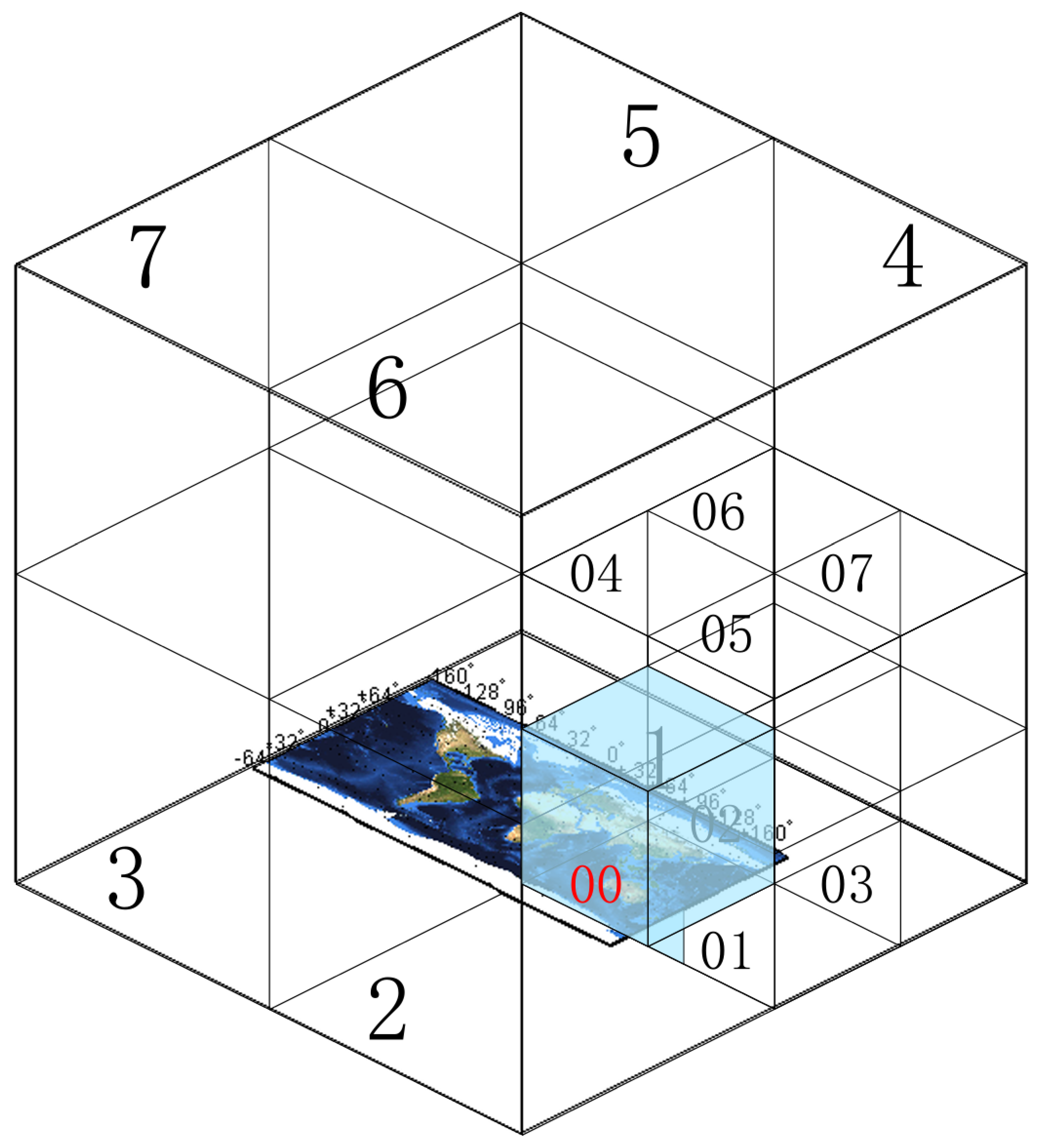
GeoSOT-3D adopts three-dimensional Z-order encoding, in which the binary bits of longitude, latitude, and elevation are interleaved bit by bit in Morton order to form a one-dimensional integer code [61], as shown in Figure 9. The fundamental design principle is to transform complex floating-point three-dimensional spherical coordinates into integer bit operations based on a 2ⁿ-tree structure. By extending Earth space into a 512° × 512° × 512° virtual cube, the three coordinate directions can be strictly aligned within a unified integer coordinate system. This design has demonstrated high engineering efficiency in massive spatial data retrieval and low-altitude airspace management for the low-altitude economy [50].

However, the Z-order curve has an inherent “Z-shaped jump” problem: for certain spatially adjacent voxels, their encoding values may differ far more than expected. As a result, spatial locality cannot be strictly guaranteed in code-range-based spatial queries.

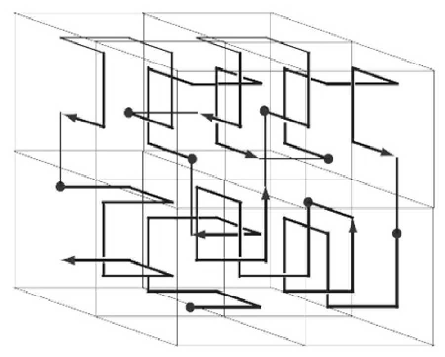
S³G adopts the three-dimensional Hilbert curve, which provides better clustering performance [24], as shown in Figure 10. Compared with the Z-order curve, it alleviates discontinuous jumps and therefore offers computational advantages in neighborhood retrieval. The modular layer-based organization of S³G further gives its encoding system distinctive flexibility, allowing different Earth system layers to employ mutually independent Hilbert encoding schemes. Nevertheless, Hilbert encoding depends on high-dimensional state-transition tables, and its maintenance cost increases significantly with dimensionality. This limits its scalability in ultra-large-scale parallel computing. Moreover, when handling cross-level data access in ESSG, the algorithm struggles to maintain consistent clustering effects, causing its locality advantage to weaken or even fail along the radial dimension.

SDOG designs a specialized Degenerated Z-order curve (DZ curve) for the irregular topology of the sphere degenerated octree [22,23]. In SDOG, the “degeneration” operation near polar regions reduces subdivisions that would normally generate eight child voxels into four or two child voxels, meaning that standard Z-order encoding cannot be directly applied. The DZ curve assigns special code prefixes to degenerated cells, ensuring that degenerated and non-degenerated cells at the same level do not conflict. At the same time, parent–child containment relationships can still be directly inferred from code prefixes. On this basis, the DZ curve is divided into two forms. SDZ (Single hierarchical DZ) is a static, single-resolution scheme with a simple encoding structure and fast decoding speed. It is suitable for scenarios with fixed subdivision levels, such as global seismic tomography parameterization. MDZ (Multiple hierarchical DZ), by contrast, embeds explicit level identifiers into the code, allowing grid cells at different levels to coexist dynamically and without conflict within the same indexing system. It supports adaptive-resolution three-dimensional spatial data organization. For example, fine-grained voxels can be used in geologically complex regions, while coarse-grained voxels can be used in homogeneous regions, with both coexisting unambiguously in the same coding space. This capability is of great value for multi-scale three-dimensional modeling of the global lithosphere.

The choice of encoding method must be closely coupled with the underlying subdivision geometry. The Z-order encoding of GeoSOT-3D is highly compatible with its integer coordinate system based on the virtual cube. The DZ curve of SDOG is specifically designed for the irregular topology of the degenerated octree. The Hilbert curve of S³G serves the cross-layer locality requirements of its modular spherical-shell structure. In addition, the ability to support multi-resolution coexistence is a key indicator of the engineering value of an encoding scheme. The single-resolution limitation of SDZ makes it difficult to adapt to the multi-scale heterogeneity of real Earth system data, whereas MDZ addresses this issue through variable-length encoding.

4.2. Hybrid Encoding Methods

Hybrid encoding methods integrate hierarchical structure encoding with coordinate-axis encoding. They decompose the identifier of a three-dimensional voxel into several semantically explicit coding components, independently encoding dimensions such as spherical position, radial depth, and layer affiliation, before concatenating them into a complete identifier according to specific rules. SGOG, SGDOG, and ISEA4H-ESSG are typical representatives of this category. All originate from the encoding requirements of three-dimensional extensions based on polyhedral grids, but they differ significantly in component design and dimensional organization.

SGOG was the first to decompose the identifier of a three-dimensional voxel into four independent components: a layer code in hexadecimal, an octant identification code in octal, a spherical position code using fixed-direction quaternary encoding, and a radial depth code in binary [25]. This established the basic paradigm of “dimension separation and domain-specific encoding.” The introduction of the layer code enables rapid localization of layer positions from the Earth’s center to the magnetosphere, meeting the needs of multi-layer data organization in Earth system science. The radial depth code and spherical position code provide encoding-level flexibility for unequal radial subdivision and adaptive spherical refinement. However, SGOG’s four-part encoding contains a degree of redundancy. Layer information can essentially be implied by radial depth, and spherical encoding and coordinate transformation must be performed in separate steps, increasing computational complexity. Building on SGOG’s octant identification and hierarchical domain-partitioning strategy, SGDOG simplifies and optimizes the encoding structure. SGDOG adopts a three-part hierarchical encoding structure consisting of an octant ID (I), radial depth code (J), and spherical position code (K) [30]. It removes the independent layer code and integrates its function into the radial depth code. By first uniformly dividing the radius and then calculating the radial interval index, the radial code naturally carries layer semantics. Meanwhile, SGDOG replaces the fixed-direction spherical position encoding with Goodchild encoding and uses the ETP distance comparison method to directly transform longitude and latitude into spherical codes. This improves the consistency between encoding and coordinate transformation, making the method practically valuable for multi-layer three-dimensional modeling and Digital Earth three-dimensional tiling scenarios.

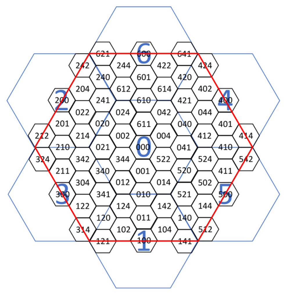
The encoding system of ISEA4H-ESSG is more refined, consisting of three mutually independent components: layer-surface code, layer-radius code, and temporal code [29], as shown in Figure 11. The layer-surface code uses a hexagonal three-axis coordinate system, in which integer coordinates (q,r,s) along three non-orthogonal axes satisfy q + r + s = 0 to uniquely identify hexagonal cells. Combined with OHQS hierarchical quadtree subdivision, this approach fully exploits the tri-axial symmetry of icosahedral hexagonal grids and avoids the coordinate ambiguity of traditional row-column indexing. The layer-radius code adopts an l − k dual-parameter format, where l denotes the total radial subdivision level and k denotes the radial index of the voxel at level l. This allows voxels with different radial resolutions to coexist unambiguously within the same coding space and supports the radial degenerated subdivision mechanism, effectively balancing grid-resolution differences between inner and outer layers. The temporal code adopts a multi-resolution hierarchical code, providing a clear interface for four-dimensional grid (4D-DGGS).

The core advantages of hybrid encoding methods lie in semantic readability and dimensional extensibility. By decomposing three-dimensional voxel identifiers into multiple independent components, these methods are not only easier for humans to understand and debug, but more importantly, they reserve a clear interface for temporal extension. By simply appending a temporal coding component, the system can evolve toward a four-dimensional spatiotemporal grid without requiring a fundamental reconstruction of the existing three-dimensional encoding framework.

However, multidimensional composite structures also impose higher requirements on database index design. How to preserve the independent retrievability of each component while enabling efficient three-dimensional joint queries remains the main challenge for the engineering implementation of hybrid encoding methods.

4.3. Comparative Analysis and Scope of Encoding Methods

The preceding subsections describe each scheme largely in isolation. To enable a systematic and, where possible, quantitative comparison, this subsection first consolidates the space-filling-curve schemes along common criteria, then details the field structure of the three hybrid schemes, and finally distinguishes code-space locality from true topological adjacency and clarifies the scope of encoding as a foundation for data management.

Table 3. Comparison of space-filling-curve-based encoding schemes.

Criterion	Z-Order (GeoSOT-3D) [61]	Hilbert (S3G) [24]	Degenerated Z-Order (SDOG) [22,23]
Underlying grid	integer cube, 2n-tree	Layered spherical shells	Degenerated octree
Code length	d·n bits	d·n bits	SDZ: 4 ≤ L ≤ 3n + 3; MDZ: L = 3n + 3
Encoding principle	Morton	state-table dependent	DZ prefix on degenerated cells
Encoding/decoding cost	O(n)	O(n)	MBG addressing O(n)
Prefix parent–child hierarchy	Yes, from prefix	Not prefix-preserving	Yes; containment from prefix
Locality preservation	Moderate	Stronger than Z-order	Moderate; constrained by degeneration
Multi-resolution coexistence	Limited	Limited	MDZ: yes; SDZ: no

compares the two space-filling-curve families along criteria for which the literature provides closed-form or measured values. Here n denotes the subdivision level and d the number of interleaved spatial dimensions.

For the degenerated Z-order family the quantitative characterization is the most complete. The multi-resolution code length grows linearly with level as L_MDZ = 3n + 3, while the single-resolution code satisfies 4 ≤ L_SDZ ≤ 3n + 3; coding time, decoding time and code length are all nearly linear functions of the subdivision level, and the practical differences among schemes remain within a few microseconds and of the same order of magnitude. At the algorithmic level the SDOG addressing operations are efficient: computing the MDZ code for the minimum bounding grid has time complexity O(n), and generating the triple representation of an object has time complexity O(2^m), where m is the maximum subdivision level of the boundary or interior grids [58].

The three hybrid schemes differ in the number of fields, the radix of each field, and the semantics carried by the radial dimension.

Table 4. Field structure of the three hybrid encoding schemes.

Model	Component Fields	Code Length	Temporal Field
SGOG [25]	Layer + octant + spherical position + radial depth	variable	none
SGDOG [30]	octant ID I + radial depth J + spherical position K	3 + nlevel + 2n bits	none
ISEA4H-ESSG [29]	layer-surface + layer-radius + temporal	variable	hierarchical temporal code

therefore lists their field structures explicitly. The trend from SGOG through SGDOG to ISEA4H-ESSG is one of progressive simplification and functional enrichment: the redundant layer field of SGOG is absorbed into the radial code in SGDOG, and a dedicated temporal field is added in ISEA4H-ESSG.

For the polyhedral hybrid grids, SGOG stacks QTM cells with a fixed radial rule, and its area ratio converges to about 2 while the degenerated area ratio converges to about 2.22; under equal-length radial stacking its cell volumes do not converge, whereas an unequal-length radial rule restores a converged volume ratio. SGDOG improves on this: its volume ratio converges to 8.43, smaller than the value 8.89 of SDOG, while GeoSOT-3D diverges with level [26]. Regarding encoding efficiency, the SGDOG address code can be encoded and decoded in real time, but efficiency decreases with level because the number of code bits grows with the level, and encoding is consistently slower than decoding because the ETP conversion used in encoding requires determining the direction and computing with irrational numbers and exponents. For ISEA4H-ESSG, the hexagonal tri-axial encoding combined with radial degeneration has been reported to yield neighbourhood-retrieval efficiency about 20% higher than H3 in three-dimensional modeling of the ionosphere and the global atmospheric temperature field.

A distinction that these code-length and complexity figures can easily obscure is that numerical proximity in the code space is not equivalent to true topological adjacency between cells. This is a known property of space-filling curves. For the Z-order curve, proximity is not always preserved, since points that are close in the Z-curve sequence may not be adjacent in space; this is precisely the origin of the “Z-jump”. The Hilbert curve preserves stronger spatial proximity than the Z-order curve, yet it still cannot guarantee that all topological neighbours remain contiguous in the linear ordering. The degeneration of SDOG and the non-orthogonal radial partition of the icosahedral hybrid schemes further weaken the correspondence between code adjacency and cell adjacency, especially across degeneration cores and along the radial direction. Consequently, a code-range query recovers an approximation of a spatial neighbourhood rather than its exact topological closure, and rigorous neighbour retrieval must still rely on an explicit adjacency rule defined on the grid geometry rather than on the linear code alone. This distinction is essential whenever an encoding scheme is used as the basis for neighbourhood-dependent operations such as buffer analysis, flux exchange, or graph-based spatial learning.

Finally, it must be emphasized that an encoding method alone does not guarantee efficient database queries or distributed processing; performance additionally depends on the indexing implementation, the storage architecture, and the query workload. Integrating the same GeoSOT encoding with different database engines yields markedly different gains—for example, its combination with PostGIS improves overall query performance by up to about 40%, while integrating a GeoSOT-based grid management method with a commercial spatial database improves retrieval efficiency by about 48% relative to traditional indexing [33]. In distributed environments the benefit of a locality-preserving code is realized only when it is aligned with the physical storage order: by using spatiotemporal identifiers as row-key prefixes and exploiting lexicographically ordered row-key storage, spatially and temporally adjacent data are placed closer in physical storage, significantly reducing disk-seek operations. A locality-preserving code such as Hilbert therefore reduces the number of disjoint code ranges a range query must scan, but this advantage can be negated by an index structure or a sharding scheme that is misaligned with the code order. The encoding schemes reviewed here should accordingly be understood as a necessary foundation for, rather than a sufficient guarantee of, efficient spatial data management, and their engineering value can only be assessed together with the indexing, storage, and workload context in which they are deployed. Throughout this review we distinguish two categories of claim. Theoretical encoding properties—such as integer bit-operation indexing, prefix-based parent–child inference, O(n) encoding/decoding complexity, and the uniform adjacency of hexagonal cells—follow deterministically from a scheme’s construction and hold independently of implementation. Experimentally demonstrated query performance—such as reported retrieval speedups, percentage improvements over H3, or database-level query gains—is by contrast conditional on the dataset, baseline, computing environment, and metric of the originating study. Because the primary sources reviewed here were evaluated under heterogeneous and often incompletely specified conditions, the quantitative performance figures reported above are not directly comparable across models and are presented as single-study, indicative results. A rigorous cross-model benchmark on a common dataset, baseline, and hardware environment remains an open task and a prerequisite for any definitive performance ranking.

5. Application Domains

This section turns to how these intrinsic properties translate into practical suitability. We organize the discussion around a requirement–property–grid logic: each application domain imposes a dominant set of requirements, deterministic and reproducible addressing, or stable neighbourhood structures—and these requirements are met by grids whose geometric and encoding properties are aligned with them.

Table 5. Requirement–property–grid mapping across ESSG application domains.

Application Domain	Dominant Requirement	Typical Data	Computational Demand	Representative Suitable Grids	Key Limitation
Geophysics & geodynamics	Adaptive radial resolution; bounded volume ratio	Travel-time residuals; velocity/gravity fields	Well-conditioned volumetric integrals	SDOG; SGDOG; Spiral Grid	Costly radial neighbour arithmetic
Atmospheric & space sciences	Conservation; low anisotropy	State fields; MHD fields; GNSS-RO	Long-time conservation; tight CFL	SCVT/MPAS; Yin–Yang; ISEA4H-ESSG	Overlap-zone interpolation; no persistent code
Smart cities & digital twins	Deterministic addressing; GIS/BIM compatibility	3D/voxel models; point clouds; sensor streams	Real-time integer indexing; LOD	GeoSOT-3D	Polar/centripetal distortion
Spatial intelligence & big data	Stable, regular neighbourhood	Voxel tensors; graph-structured data	Fixed message-passing support	GeoSOT-3D; SEGS	Code proximity ≠ adjacency

consolidates this mapping, linking each domain to its dominant grid requirements, the associated data types, the principal numerical or computational demands, the grid families aligned with it, and the documented limitations that constrain that suitability. In the following subsections we review representative work in each domain and, for each, make explicit why particular grid properties render certain approaches suitable.

5.1. Geophysics and Geodynamics

Geophysics and geodynamics represent one of the most mature traditional application domains of ESSG. Their core requirement is high-precision global-scale numerical simulation of complex physical fields and material flows inside the Earth. In mantle convection and plate tectonics research, researchers have used icosahedral or spiral grids to construct global mantle convection models, effectively avoiding the singularity problem of conventional latitude–longitude grids at the poles and significantly improving simulation accuracy and computational stability [62]. In seismology and tomography, multi-resolution three-dimensional spherical grids have been used for seismic-wave travel-time calculation and global mantle P-wave velocity structure imaging. Their adaptive refinement capability makes it possible to achieve local high-resolution representation in tectonically complex regions such as subduction zones [21,54]. In addition, forward gravity-field modeling methods based on discrete global grid cells such as hexagonal prisms provide a unified spatial reference framework for high-precision numerical modeling of global and regional gravity fields [63,64]. In geomagnetic and electromagnetic induction simulations, spherical grids support fine-scale characterization of global electromagnetic induction effects and the spatial distribution of the geomagnetic field [65]. For three-dimensional lithospheric structures, the SDOG enables multi-scale representation and visualization of the global lithosphere, providing an effective data organization method for deep geological interpretation [57].

The grid properties underlying this suitability are twofold. First, geodynamic processes are governed by strong radial heterogeneity—true Earth discontinuities such as the Moho and the core–mantle boundary act as physical anchors—so the decisive requirement is adaptive radial resolution together with the ability to constrain radial nodes onto these interfaces, as exploited by Ballard et al. [54]. Volumetric grids with an explicit geocentric-singularity treatment (SDOG) and depth-adaptive shell-based grids (SGDOG) satisfy this requirement while bounding the volume-ratio degeneration analyzed in Section 3.6, which is essential because tomographic inversion and gravity forwarding require cell volumes to remain comparable for the discretized integrals to stay well-conditioned. Second, mantle-flow solvers demand compact, quasi-uniform cells with low anisotropy; the near-unity volume ratio and high sphericity of Voronoi-based meshes make them preferable for the PDE-oriented end of this domain, at the cost of relying on stored adjacency rather than a decodable global identity.

5.2. Atmospheric and Space Sciences

In numerical weather prediction and atmospheric modeling, the Yin-Yang grid and the Voronoi-grid-based MPAS-A platform have been used to construct nonhydrostatic atmospheric dynamics models. While ensuring uniform global coverage, these approaches effectively improve numerical accuracy in polar regions [50,61]. In multi-resolution climate system simulation, spherical centroidal Voronoi tessellation (SCVT) has been applied to coupled simulations of interactions among ice sheets, oceans, and the atmosphere. Its variable-resolution characteristics make local refinement possible in key regions [60]. In coronal and space-weather simulation, the Yin-Yang grid has been used for global coronal magnetohydrodynamic (MHD) simulations, providing an efficient computational framework for space-weather prediction [51]. In addition, ionospheric three-dimensional modeling and global atmospheric temperature-field formatting based on the ISEA4H-ESSG model assign unified grid identifiers to massive spaceborne GPS radio occultation data and ground-based observation data. This enables real-time assimilation and high-fidelity interpolation of space-environment parameters at the global scale [29].

The property that dominates atmospheric modeling is conservation combined with low anisotropy. Because atmospheric dynamical cores solve conservation laws over long integration times, the grid must minimize spurious numerical dispersion arising from cell-shape irregularity: this favours compact, quasi-uniform cells such as the near-hexagonal SCVT cells that MPAS couples with C-grid staggering, and it explains why the polar convergence of latitude–longitude grids—which introduces both a stringent time-step restriction and directional anisotropy—is disqualifying for global dynamical cores. The Yin–Yang grid removes the polar singularity geometrically and is therefore well suited to MHD and NWP, but its overlap zone requires interpolation for flux exchange, a limitation directly traceable to its intent-B, non-persistent-identity profile in Table 1. In contrast, space-environment assimilation is dominated by a different requirement—deterministic addressing of massive multi-source observations—for which the encoding-enabled ISEA4H-ESSG is suited, its radially degenerate hexagonal indexing yielding neighbourhood-retrieval efficiency reported at about 20% above H3.

5.3. Smart Cities and Digital Twins

With the rapid development of urban informatization and digital twin technologies, ESSG has gradually become an important underlying spatial framework for city information models. In urban model lightweighting, generative level-of-detail (LOD) algorithms based on integrated space–air–ground grid models significantly improve rendering efficiency and data loading speed for large-scale urban scenes through hierarchical grid encoding of three-dimensional urban elements [66]. For ubiquitous location information management, the Geographic Grid Region Name (GGRN) mechanism provides efficient spatial indexing and retrieval for the location information of massive sensor nodes and mobile devices, effectively supporting real-time management of smart-city sensing data [48]. In the integration of three-dimensional building and point-cloud data, associative mapping between voxel models and GeoSOT-3D grids enables integrated indoor-outdoor positioning and visual representation. This provides a unified spatial reference for the deep integration of Building Information Modeling (BIM) and Geographic Information Systems (GIS) [67,68].

The decisive property for digital twins is deterministic, reproducible addressing. A digital twin must guarantee that a given physical location maps to the same cell identifier across platforms, sensors, and time, so that heterogeneous urban data streams can be fused and updated in real time; this requirement is met by intent-A frameworks with closed-form integer encoding, of which GeoSOT-3D is the canonical example, since its 2ⁿ-tree Z-order code reduces spatial queries to integer bit operations. Equal-volume behaviour, which is critical for geophysics, is largely irrelevant here; instead, compatibility with conventional GIS and voxel/BIM data models is paramount, which is why latitude–longitude-inheriting grids remain the practical choice despite their polar and centripetal distortion, since urban applications operate far from both the poles and the geocentre where that distortion becomes severe.

5.4. Spatial Intelligence and Big Data Management

In spatial intelligence and big data management, ESSG provides a regularized discrete spatial indexing structure that supports efficient organization and intelligent analysis of large-scale geospatial data. In the construction of spatial intelligence frameworks, GeoSOT-3D grids provide standardized coding mechanisms and neighborhood embedding matrices, effectively supporting spatiotemporal reasoning models and cross-domain transfer learning [69]. In three-dimensional spatial analysis, buffer algorithms based on three-dimensional Discrete Global Grid Systems overcome the limitations of traditional two-dimensional buffer analysis and enable accurate neighborhood-relation computation for complex three-dimensional spatial objects [70]. In multi-scale data organization and indexing, elastic grid structures (SEGS) [71] and adaptive Hilbert-Geohash encoding schemes significantly improve storage efficiency [72], query response speed, and dynamic update capability for massive geospatial data through hierarchical organization of three-dimensional voxel data. On the application side, DGGS have been adopted as the standard data fabric for integrating heterogeneous geospatial data into machine-learning workflows: Li et al. [73] coupled an ISEA3H hexagonal DGGS with external learning algorithms to project multi-scale flood risk across climate-change scenarios, demonstrating the viability of DGGS as a scalable, multi-resolution substrate for environmental prediction. Similarly, Liu et al. [74] introduced a Discrete Satellite Gridding Neural Network that maps grid-cell positional information into a standardized vector representation, substantially raising the spatial resolution and fusion accuracy of satellite ocean data, and highlighting the affinity between discrete grid structures and neural-network-based learning models. In the management of spatiotemporal Earth observation data, DGGS-based multiresolution frameworks have recently been extended to live updating, real-time retrieval over arbitrary regions of interest, and smooth approximation of missing observations for global satellite imagery, demonstrating the scalability of discrete grid organization to continuously growing observation streams [75].

The property that governs spatial-AI suitability is a stable, regular neighbourhood structure. Graph- and grid-based learning models propagate information through fixed adjacency relations, so the grid must provide uniform, deterministic neighbourhoods that can serve as a well-defined message-passing support and as a neighbourhood embedding matrix; hierarchical intent-A grids with regular parent–child and adjacency arithmetic (GeoSOT-3D) satisfy this requirement, whereas the irregular, explicitly stored adjacency of unstructured meshes does not readily furnish the fixed-size neighbourhoods such models assume. A residual limitation, emphasized in Section 4.3, is that code-space proximity is not identical to topological adjacency; neighbourhood-dependent learning must therefore rely on an explicit adjacency rule rather than on code ranges alone.

6. Challenges and Prospects

Although Earth System Spatial Grid has made significant progress in both theory and application, several challenges remain before they can fully serve as the foundation for next-generation multiphysics coupling and digital-twin Earth systems.

Rigorous adaptation to the real Earth. Precise adaptation to the real Earth requires distinguishing three nested reference figures that are frequently conflated: the mathematical sphere on which the tessellation algebra is defined, the reference ellipsoid that provides a rigorous geodetic datum, and the physical Earth whose surface follows the geoid and the true topography. Nearly all of the three-dimensional models reviewed here are constructed on the mathematical sphere, and the central open problem is not merely that the Earth is ellipsoidal but whether a hierarchical sphere-to-ellipsoid transformation can simultaneously preserve the properties that make a DGGS useful—approximate equal area/volume, adjacency, parent–child hierarchy, compactness, and a closed indexing algebra. These properties are generally in tension: a mapping that restores equal area on the ellipsoid typically perturbs cell shape and the integer coordinate arithmetic on which fast indexing depends. The problem is therefore best framed in terms of the mapping properties of the sphere-to-ellipsoid transformation, and prior WGS84-based hierarchical subdivision, such as QTM on the WGS84 ellipsoid [39], has already shown that the choice of transformation directly determines which of these properties survive refinement. Establishing a datum-aware, property-preserving three-dimensional transformation on a rigorous geodetic ellipsoid remains a mathematical problem requiring further breakthroughs.

Well-defined vertical semantics and cross-sphere integration. A three-dimensional Earth-system grid requires an explicit definition of its reference surface, coordinate reference system, radial coordinate, and vertical datum, because “radial extension” otherwise conflates several physically distinct vertical references. The geocentric radius natural to sphere-based volumetric grids such as SDOG differs from the ellipsoidal height measured along the ellipsoidal normal required by GNSS positioning, from the orthometric height referenced to the geoid used in engineering and hydrology, from the physical depth below the surface used in solid-Earth and lithospheric modelling, and from the geopotential- or pressure-based atmospheric levels used in meteorology and space science. These references are not interchangeable, and the quantities relating them are of different dimensional character. The geoid undulation N is a linear separation between the geoid and the reference ellipsoid, expressed in metres and reaching magnitudes on the order of tens of metres that vary geographically; the deflection of the vertical, by contrast, is an angular quantity representing the angle between the direction of the plumb line (gravity vector) and the ellipsoidal normal, and is expressed in arcseconds. Because these vertical references differ by such linear and angular amounts, a grid that silently equates geocentric radius with ellipsoidal or orthometric height introduces systematic vertical misregistration when integrating cross-domain observations. Consequently, the compatibility of each grid family with these vertical concepts is application-specific. Sphere-based volumetric grids (SDOG) and shell-based polyhedral grids (SGOG, SGDOG, ISEA4H-ESSG) are most naturally parameterized by geocentric radius, which suits geodynamic and mantle-convection applications where the deep interior and true Earth discontinuities such as the Moho and the core–mantle boundary are the relevant radial anchors, as exploited by radial partitions constrained to lie on such discontinuities [54]. GNSS and gravity-field modelling instead require the grid to be expressible in ellipsoidal height and geoid-referenced quantities, so that satellite orbit tracking, occultation profiles, and gravity functionals share a rigorous datum. Atmospheric and space-weather grids, such as the ionospheric and temperature-field applications built on ISEA4H-ESSG [29], operate most naturally on geopotential or pressure levels, whose spacing is neither uniform in radius nor equal in volume. Cross-sphere integration therefore depends on defining explicit, invertible transformations among these vertical references and on ensuring that each cell identifier is unambiguously associated with a formally defined grid reference system and its datum/CRS.

From conceptual standardization toward implementation and interoperability. The second edition of the OGC Abstract Specification Topic 21—Discrete Global Grid Systems (OGC Topic 21 v2.0, standardized as ISO 19170-1:2021) [31] extends the DGGS Core to support up to three spatial dimensions and one temporal dimension and introduces the concept of a zone as a region of space–time. Conceptual standardization for three-dimensional and spatio-temporal DGGS thus already exists at the abstract-specification level, and the remaining challenges concern implementation, interoperability, conformance assessment, and adoption. Most existing DGGS libraries pre-date the current abstract specification and only partially satisfy its requirements, and the widely deployed specifications in practice still target two-dimensional equal-area DGGS of the Earth’s surface. The publication of the OGC API—DGGS implementation standard and the establishment of a register for DGGS reference-system definitions are important steps toward closing these gaps, but conformance-tested three-dimensional and equi-volumetric implementations, together with agreed metadata, topological interfaces, and cross-grid exchange protocols for volumetric cells, remain to be established and adopted. This assessment is echoed by a recent review of spatial-grid interoperability, which identifies the difficulty of interoperating between heterogeneous grids defined on different reference surfaces, the lack of interoperability methods for volumetric and spatiotemporal grids, and the absence of rigorous reliability evaluation of grid conversion as the key obstacles to multi-source data fusion [76].

Reconciling reference-indexing and numerical-discretization lineages. Unstructured numerical meshes such as the Spiral Grid and SCVT/MPAS, and encoding-enabled polyhedral grids such as ISEA4H-ESSG, are converging from opposite directions. A concrete open problem is to endow adaptive Voronoi-style cells with a deterministic, decodable identity, so that adaptive simulation meshes and reproducible spatial-indexing frameworks can be addressed and exchanged through a common algebra.

Beyond the challenges above, several wider directions are worth noting, with the caveat that their connection to the specific limitations reviewed here is more exploratory. First, in big-data and cloud-computing environments, existing grid-encoding logic can conflict with distributed-storage layout and parallel-computing scheduling; aligning hierarchical cell encoding with cloud-native storage and execution models is a natural engineering direction. Second, and more speculatively, the regular, hierarchical, and neighbourhood-explicit structure of ESSG cells may provide a well-defined discrete support for learning-based spatial models, such as graph or grid neural networks whose message passing follows the grid’s parent–child and adjacency relations. We present this as a possible avenue rather than a necessity: it is motivated by the structural affinity between grid topology and graph-based learning, but it does not follow directly from a limitation identified in the reviewed literature, and its practical value for Earth-system tasks remains to be demonstrated. Finally, the evolution toward 4D-DGGS will introduce recursive subdivision along the temporal dimension; the space–time zone concept of OGC Topic 21 v2.0 and the temporal-code interfaces already present in models such as ISEA4H-ESSG provide a concrete starting point, so that grid systems may eventually capture dynamic Earth-system processes—such as extreme-climate evolution and plate motion—with long-term continuity.

7. Conclusions

This review has traced the evolution from two-dimensional DGGS to the three-dimensional Earth System Spatial Grid (ESSG), providing a unified comparative analysis of shell-based, volumetric, and unstructured approaches across their geometric construction, radial extension, encoding, and applications.

Three comparative findings stand out. First, three-dimensional extension is not the addition of an independent radial axis but a problem of jointly controlling angular and radial degeneration; among reference-indexing frameworks, the volumetric SDOG—by treating the geocentric singularity as an explicit design object—is representative of grids that combine exact addressing with bounded volume variation. Second, models sharing a single geometric label often differ fundamentally once separated by design intent—reference-indexing frameworks (intent A) versus numerical-discretization meshes (intent B)—a distinction that the six-dimensional classification matrix makes explicit and that explains why grids such as GeoSOT-3D and MPAS are not directly comparable. Third, application suitability follows a coherent requirement–property–grid logic, whereby each domain’s dominant requirement selects the grid family whose geometric and encoding properties are aligned with it.

The specific contribution of this review is threefold: to the best of the authors’ knowledge, it offers the first unified comparison spanning the full ESSG spectrum rather than treating each class in isolation; it introduces a multidimensional framework that separates a grid’s design intent from its geometry, hierarchy, indexing, cross-layer topology, and numerical role, thereby resolving the ambiguities of single-axis taxonomies; and it consistently distinguishes construction-derived theoretical properties from implementation-dependent performance claims, providing a reproducible basis for application-driven grid selection. Building on the open challenges identified in Section 6, these contributions are intended to support the future development of a standardized, interoperable, four-dimensional spatiotemporal grid framework.