


Abstract
With the rapid development of the Internet of Things (IOT), 5G, and modern power systems, demand-side loads are becoming increasingly observable and remotely controllable, which enables demand-side flexibility to participate more actively in grid dispatch and emergency support. Under extreme rainstorm conditions, however, component failure risk rises and the availability and dispatchability of demand-side flexibility can change rapidly. This paper proposes a risk-aware emergency regulation framework that translates rainstorm information into actionable multi-load aggregation decisions for urban power systems. First, demand-side resources are quantified using four response attributes, including response speed, response capacity, maximum response duration, and response reliability, to enable a consistent characterization of heterogeneous flexibility. Second, a backpropagation (BP) neural network is trained on long-term real-world meteorological observations and corresponding reliability outcomes to estimate regional- or line-level fault probabilities from four rainstorm drivers: wind speed, rainfall intensity, lightning warning level, and ambient temperature. The inferred probabilities are mapped onto the IEEE 30-bus benchmark to identify high-risk areas or lines and define spatial priorities for emergency response. Third, guided by these risk signals, a two-level coordination model is formulated for a load aggregator (LA) to schedule building air conditioning loads, distributed photovoltaics, and electric vehicles through incentive-based participation, and the resulting optimization problem is solved using an adaptive genetic algorithm. Case studies verify that the proposed strategy can coordinate heterogeneous resources to meet emergency regulation requirements and improve the aggregator–user economic trade-off compared with single-resource participation. The proposed method provides a practical pathway for risk-informed emergency regulation under rainstorm conditions.
1. Introduction
Demand-side response (DR) emerged in the United States alongside electricity market reforms to leverage demand-side resources and enhance system reliability [1]. During periods of price volatility or system stress, system operators or end users may temporarily adjust consumption in response to price signals or incentives. Such actions reduce or shift demand within a specified time window, helping maintain grid stability and mitigate short-term price spikes [2]. Emergency response (ER) involves issuing alerts to users based on predefined emergency levels when the power grid is at risk of collapse, requesting load reductions. Participants in ER are compensated by the operator according to a pre-agreed compensation plan [3].
Extreme weather can disrupt electricity supply for millions of people and severely challenge power-system operations. For example, the 2008 La Niña event lowered Pacific sea-surface temperatures and contributed to an unusually severe snowstorm in China. The event disrupted electricity use for approximately 77 million people nationwide. In 2020, a major extreme-weather event in California reduced solar generation. Meanwhile, elevated summer temperatures sharply increased electricity demand, resulting in rotating (rolling) outages that affected at least 810,000 households [4]. In 2021, a cold wave in Texas triggered a large-scale power outage, affecting more than 1.4 million households.
Extreme weather disrupts daily life and poses major challenges to grid stability, especially in systems with high renewable penetration. As meteorological hazards become more frequent, the vulnerability of power systems has attracted growing attention worldwide. Several studies have systematically reviewed meteorological hazards affecting China’s power grid, and representative advances are summarized below. Wang et al. [5] examined the resilience of integrated gas–power systems under extreme weather and proposed a quantitative framework for vulnerability assessment. To enhance robustness against extreme events, Zare et al. [6] developed a co-planning approach for generation and transmission expansion that explicitly accounts for uncertainty in resilience-related resources. Focusing on failure propagation, Lian et al. [7] proposed a resilience assessment method based on cascading-failure graphs to analyze extreme-weather-induced disturbances. With advances in sensing and communication, research has increasingly focused on enhancing resilience through situational awareness and intelligent coordination. Nair et al. [8] demonstrated that trustworthy IoT-coordinated assets can enhance grid resilience under extreme conditions. From a decision-making perspective, Ghahramani et al. [9] proposed a risk-averse, data-driven distributionally robust optimization method for transmission systems, enabling conservative yet adaptive operation under uncertainty. Mahmoud et al. [10] systematically reviewed predictive maintenance in smart distribution networks, summarizing fault types, causes, and prediction methods; this review provides a foundation for fault prediction and risk identification to support resilience under adverse weather conditions.
However, rainstorm-driven disturbances pose an additional, often overlooked challenge: beyond increasing outage risk, rainstorms also reshape the demand-side conditions that emergency regulation depends on. First, rainstorm-related changes in temperature and occupancy/behavior can shift the net-load baseline and reduce the curtailment headroom of building loads. Second, heavy precipitation and cloud cover can reduce photovoltaic (PV) output, while mobility disruptions and severe-weather alerts can change electric vehicle (EV) plug-in availability and controllability [11]. Consequently, the effective aggregatable flexibility during rainstorms may differ substantially from that under normal conditions. Emergency regulation should therefore account for these storm-dependent changes rather than treating the demand side as static. This motivates the central role of multi-load aggregation in our study. Aggregation enables fast and reliable mobilization of heterogeneous flexibility at scale, improves robustness to individual uncertainty or unavailability, and supports implementable emergency dispatch and settlement at the aggregator level [12].
With large-scale renewable integration, especially distributed photovoltaic systems, power-system operation becomes increasingly sensitive to weather-induced uncertainty, which motivates robust assessment and flexible demand-side coordination. Yang et al. [13] proposed a robust method for assessing distributed PV hosting capacity in alternating Current (AC)/Direct Current (DC) hybrid distribution networks by introducing a spatiotemporally dependent polyhedral model and incorporating demand response to mitigate PV-output uncertainty. Ma et al. [14] further investigated hybrid energy-storage configuration optimization in distribution networks with high PV penetration, explicitly considering user-side demand response to improve system flexibility and economic performance. To address load imbalance, Wang et al. [15] developed a distributionally robust demand response model that coordinates heterogeneous household appliances to mitigate peak-to-valley disparities driven by rooftop PV integration and increasing heating demand in cold climates. Zhang et al. [16] investigated a robust-optimization-based scheduling framework for microgrids and electric-vehicle demand response, improving operational flexibility and economic efficiency under uncertainty. Overall, prior studies have made substantial progress in resilience assessment, fault prediction, and demand response modeling. Nevertheless, an end-to-end operational linkage that connects evolving extreme-weather risk (especially rainstorms) to targeted emergency regulation with coordinated multi-load aggregation remains insufficiently explored. To position this work, Table 1 summarizes representative studies and highlights this paper’s contributions toward addressing the above coupling gap.
Table 1.
Representative related studies and contributions of this work.
Neural networks are mathematical models inspired by biological neural systems and are widely used for distributed, parallel information processing. They process information by adjusting connection weights among many interconnected nodes. A key feature is their ability to learn from data and encode learned knowledge in synaptic (connection) weights [17]. Based on the information-flow direction, neural networks can be broadly categorized into feedforward networks, recurrent (feedback) networks, and graph neural networks. Feedforward networks have a relatively simple structure and are widely used. Among them, the backpropagation (BP) neural network is a multilayer feedforward network popularized by Rumelhart, Hinton, and Williams in 1986. It is trained using the error backpropagation algorithm and remains a widely adopted and versatile learning method.
Recent studies have increasingly applied neural networks to short-term load forecasting by incorporating exogenous variables and advanced architectures. Morais et al. [18] compared shallow and recurrent neural networks for short-term load forecasting using global climate model outputs as inputs and showed that recurrent architectures can capture climate-driven load variability. To enhance feature extraction and model tuning, Wang et al. [19] proposed a hybrid SSA–CNN–LSTM framework that jointly optimizes signal decomposition, convolutional feature extraction, and temporal modeling. Furthermore, attention mechanisms have been introduced to adaptively weight influential inputs under dynamic operating conditions. Wan et al. [20] developed an attention-augmented Long Short-Term Memory (LSTM) forecasting model to capture time-lag effects and nonlinear interactions in power-plant load dynamics.
Beyond forecasting, neural networks have been extended to demand response decision-making. Fraija et al. [21] proposed a deep reinforcement learning-based dynamic pricing framework to enable adaptive price-based demand response under market and supply constraints. In addition, recent studies have combined deep learning with decision-making and optimization methods to improve demand response performance. In particular, deep reinforcement learning-based demand response frameworks have been developed to coordinate dynamic pricing with user-side flexibility, enabling adaptive load adjustment under uncertainty (e.g., load fluctuations and external disturbances) [22,23,24]. These studies demonstrate the effectiveness of neural network-based demand response models in reducing peak load and improving operational efficiency.
Notably, extreme weather events are often localized and short-lived; meteorological drivers can emerge abruptly and intensely, causing rapid impacts on people and the environment. For example, storms can strike a region intensely within a short time window [25]. This study adopts a BP neural network to reduce training time and leverage its flexible structure for nonlinear modeling. Moreover, BP neural networks are mature and widely used. Owing to their learning and generalization capability, they can, in theory, approximate arbitrary nonlinear functions [26]. They can incorporate meteorological factors and adaptively adjust network weights and biases, thereby improving predictive performance. They can also be integrated with other algorithms to achieve specific modeling objectives [27].
To support resilient and low-carbon grid operation under rainstorm-driven disturbances, we develop a rainstorm-informed emergency-regulation framework based on multi-load aggregation. The main contributions are summarized as follows:
- To quantify heterogeneous demand-side flexibility and support dispatch under emergency regulation, we develop a multi-load aggregation framework for building air-conditioning (BAC), Distributed Photovoltaic (DP)/PV, and EV resources. We also propose a response-capability function that distinguishes response levels and enables implementable flexibility assessment and dispatch.
- To establish a data-driven mapping from rainstorm conditions to operational fault risk for emergency triggering, we develop a backpropagation (BP) neural network to estimate regional fault probabilities using rainstorm-related meteorological variables. The model is validated using a representative rainstorm event in Southern China. The estimated fault probabilities support emergency triggering and spatial prioritization, thereby enabling differentiated and targeted regulation.
- To enable actionable emergency regulation that coordinates multiple aggregated resources and promotes user participation, we propose an incentive-driven load-aggregator (LA)-coordinated regulation and allocation strategy. The proposed end-to-end workflow is validated through case studies and detailed analyses, demonstrating the benefits of coordinated multi-load participation in emergency response.
2. Demand Side Multiple Load Model and Characteristics
As shown in Figure 1, demand-side flexible resources are categorized into four groups: flexible loads, distributed generation, electric vehicles, and energy storage.
Figure 1.
Demand side flexible resource classification.
2.1. Flexible Load Aggregation Model
Flexible loads typically respond to grid control signals or electricity price signals. Based on their response mechanisms, flexible loads can be classified as incentive-based or price-based demand response resources. Temperature-controlled loads represent a typical class of flexible loads.
- (a)
- Incentive demand side resource aggregation model
The incentive-based demand response mechanism is activated when the power system is at risk of collapse. Eligible users are encouraged through financial incentives to respond to operator signals by adjusting their energy-use behavior [28]. Based on these principles, the aggregation model is formulated as follows:
where is the actual responsible power of user j participating in incentive demand response in period t; and are the minimum and maximum values of the power range that user j can respond to, respectively; j refers to the collection of users participating in incentive demand response.
- (b)
- Demand side resource aggregation model
The price-based demand response mechanism reflects system operating costs through market pricing and guides users to adjust consumption by exposing them to time-varying prices, thereby enabling efficient allocation of demand-side resources [29]. Based on these principles, the aggregation model is formulated as follows:
where is the actual responsible power of user i participating in incentive demand response mechanisms in time period t; and are the minimum and maximum values of the power range that user i can respond to, respectively. i refers to the collection of users participating in incentive demand response.
- (c)
- Temperature control load aggregation model
A temperature-controlled load has two operating states: on and standby. When the controlled temperature deviates from its setpoint, the device switches from standby to on mode. Air conditioners are typical temperature-controlled loads that provide both cooling and heating. In practice, heating technologies are diverse, whereas cooling is typically dominated by air-conditioning systems. Therefore, this study considers building air-conditioning loads as the study object.
The air-conditioning load model is established using a thermodynamically equivalent representation based on energy conservation among outdoor temperature, indoor temperature, and Heating, Ventilation, and Air Conditioning (HVAC) power. According to thermodynamic principles [30], the model incorporates indoor and outdoor temperatures, thermal capacitance, thermal resistance, and the energy–efficiency ratio. Typically, air-conditioning loads with regulation potential are aggregated using multiple air-conditioning models. Under a common temperature setpoint within a building and heterogeneous air-conditioner parameters, all units share the same steady-state state variable .
2.2. Electric Vehicle Aggregation Model
An electric vehicle aggregator (EVA) is an aggregation service provider that manages vehicle-to-grid (V2G) and grid-to-vehicle (G2V) strategies. It guides electric vehicles to adopt optimal electricity-consumption strategies via demand-side resource management, day-ahead market declarations, and real-time intra-day regulation.
The aggregated charging and discharging power of the EVA is derived from the summation of individual electric vehicle (EV) behaviors, adjusted by their respective conversion efficiencies:
where denotes the set of electric vehicles. and represent the charging and discharging power of the -th EV at time , respectively. The parameters and correspond to the charging and discharging efficiencies. Consequently, and denote the total aggregated power on the EVA side.
The dynamics of the total energy stored within the EVA are modeled by considering the previous energy state, the net power exchange, and the energy variations caused by vehicle mobility:
where signifies the total energy stored in the aggregator at time , and Δ, is the scheduling time interval. The terms and account for the energy capacity changes due to EVs connecting to (arriving) and disconnecting from (departing) the aggregator, respectively.
To ensure safe operation, the aggregated power and energy states must strictly adhere to the physical boundaries defined by the fleet’s collective capability:
where and represent the maximum aggregated charging and discharging power limits, derived from the individual EV limits and . Finally, and define the lower and upper bounds of the EVA’s adjustable energy capacity at time .
2.3. Electric Storage Aggregation Model
Distributed energy storage also relies on flexible charging and discharging. Unlike electric vehicles, its charging and discharging behavior is directly controlled by the aggregator and is not affected by external factors [31]. The aggregation model for distributed energy storage is given by (11)–(14):
where denotes the energy storage capacity at time ; and denote the charging and discharging power at time , respectively; and denote the charging and discharging efficiencies, respectively; and denote the lower and upper bounds of the storage capacity, respectively; denotes the maximum power for a single charge or discharge; and denotes the binary charging/discharging state, taking 1 for charging and 0 for discharging.
2.4. Distributed Power Aggregation Model
- (a)
- Wind turbine output model
Wind power output depends primarily on wind speed and air density and exhibits piecewise behavior with changing wind speed [32]. The wind turbine output power at time , denoted as , is given by
where denotes air density, is the wind speed at time , and is the rotor swept area. , , and are the power coefficients representing the aerodynamic efficiency of the turbine. The variable denote the cut-in, cut-out, and rated wind speeds, respectively; is the rated power of the wind turbine. The turbine does not operate when or . When , the turbine operates at rated power.
The aggregated output power of the wind turbine cluster is
where N is the number of wind turbines in the cluster.
- (b)
- Photovoltaic output model
Based on the photovoltaic effect, the PV unit output power is expressed as [33]
where is the temperature coefficient; is the ambient temperature; is the nominal operating cell temperature; is the reference temperature; is the reference efficiency; is the irradiance at time ; is the area of a single PV panel; and is the number of PV panels.
2.5. Quantitative Analysis of Emergency Demand Resources
In urban power grids with multiple responsive load groups, the effectiveness of emergency demand response (ER/EDR) depends not only on how much adjustable capacity can be provided, but also on how fast and how long the response can be sustained, and how reliable the response is in practice [34]. These attributes are widely used to characterize and accredit reliability-oriented demand response resources in market/operational practice (e.g., requirements on reaching full curtailment within a specified time and sustaining the response for several hours), and they are also consistent with common measurement-and-verification (M&V) considerations for demand response performance [35,36]. Therefore, we quantify each load group using four key attributes: response speed, response capacity, maximum response duration, and response reliability.
- Response speed is defined as the adjustable capacity delivered per unit time following receipt of dispatch instructions. High-performance resources typically respond within 5 min, whereas standard resources respond within 5–30 min. Flexible loads typically respond in more than 10 min. PV plants, wind farms, and electric vehicles typically respond within seconds to tens of seconds after receiving dispatch instructions. Energy storage resources can respond within milliseconds.
- Response capacity denotes the maximum adjustable power (load reduction and/or net injection) that a resource can provide during ER, which directly determines the maximum contribution to emergency balancing.
- Maximum response duration reflects the maximum continuous time that the resource can sustain the ER response without violating operational constraints; this attribute aligns with reliability DR designs requiring sustained response periods (e.g., at least several hours).
- Response reliability characterizes the controllability and the likelihood that a resource can be successfully converted from “available” to “dispatchable” during ER events. In this work, is quantified using the historical participation/success probability derived from past ER activations and M&V records.
The time-varying response capability of the -th load group is modeled as a trapezoidal profile (Figure 2). This profile delineates the Emergency Response (ER) process into three distinct phases: ramp-up, stable delivery, and ramp-down/exit [37]. The response power output, , is formulated as the following piecewise function [38]:
where denotes the maximum deliverable capacity. The time points , , , and define the boundaries of the response window. The intervals [, ] and [, ] correspond to the ramp-up and ramp-down periods, respectively. Their slopes represent the product of the nominal rates (, ) and the response reliability coefficient . Finally, the duration of the stable delivery phase is defined as = − .
Figure 2.
Trapezoidal function diagram.
3. Calculation of Fault Probability Based on BP Neural Network
Building upon the aggregated modeling of flexible resources in Section 2, it is imperative to address the pronounced spatiotemporal heterogeneity of grid risks intensified by extreme weather. Neglecting such spatial variations may precipitate resource misallocation and compromise regulatory efficacy. To this end, this chapter proposes a BP neural network-based approach to quantify fault probabilities by correlating meteorological variables with historical fault records. These probabilistic estimates facilitate the precise identification of high-risk zones and constitute the foundational input for the risk-oriented optimization framework detailed in Section 4.
3.1. Overall Methodological Framework
The proposed framework establishes a closed-loop methodology integrating rainstorm-driven fault risk identification with the coordinated emergency regulation of demand-side flexible resources. As illustrated in the workflow in Figure 3, the process commences with the construction of a unified dataset, synchronizing and normalizing historical demand response records with meteorological observations. Key meteorological features, including wind speed, precipitation, and lightning intensity, are extracted to train a backpropagation (BP) neural network. This model quantifies the spatiotemporal heterogeneity of grid risks, outputting regional fault probabilities that trigger subsequent decision-making.
Figure 3.
End-to-end workflow from data acquisition and fault-probability estimation to high-risk area identification and multi-load emergency regulation optimization.
Figure 4 depicts the proposed framework as a hierarchical functional model comprising three logical tiers. At the data sensing and identification tier (Level 1), the BP model processes multi-source inputs to generate real-time risk trigger signals. In the decision tier (Level 2), the load aggregator (LA) utilizes these signals to activate dynamic resource pooling for quantifying available BAC, PV, and EV capacities, followed by coordinated emergency optimization. The workflow culminates at the execution tier (Level 3), where the LA issues optimized dispatch instructions to flexible resources for system regulation. Critically, the framework incorporates a closed-loop feedback mechanism (Figure 4, right panel), which continuously monitors resource availability and regulation effects to update the system state and risk model amidst evolving weather conditions. Section 5 validates the framework’s effectiveness, accounting for scenario-dependent constraints such as PV curtailment and EV connectivity limits.
Figure 4.
Structural-functional model of a closed-loop emergency demand-side response framework.
3.2. Rainstorm Scenario and Meteorological Factors
Rainstorm events are used in this study as a representative extreme-weather disturbance scenario. To quantify weather-driven impacts on grid operation, four meteorological variables are selected as inputs for regional fault-probability estimation: wind speed, rainfall intensity, lightning warning level, and ambient temperature. Wind speed and rainfall intensity indicate the intensity of atmospheric motion and precipitation and are closely associated with flooding and equipment exposure risk [39]. Lightning warning information is included because lightning-related alarms are widely used in storm emergency operating plans. Ambient temperature is included to capture the coupled effects of weather conditions on equipment status and demand-side response.
In addition to affecting fault risk, the selected meteorological variables also shape demand-side load and flexibility during rainstorms. Ambient temperature affects BAC baseline demand and the feasible curtailment margin. Wind and rainfall conditions contribute to renewable-generation uncertainty, for example, by reducing PV irradiance. Severe-weather warnings can affect EV availability and the controllability and reliability of demand-side response. Accordingly, we updated the effective response-capacity and reliability parameters of the aggregated multi-load portfolio for each rainstorm scenario before solving the emergency-regulation optimization problem.
The meteorological variables are aligned with the demand-side response time-series using the same scheduling interval and are then normalized before model training. An initial feature set is constructed from these four variables, and their relevance is further evaluated using the correlation analysis and feature-screening procedure shown in Figure 4. These variables form the meteorological input vector for the backpropagation (BP) neural network in Section 3.3, whose output is the regional (or line/area) fault probability .
3.3. BP Neural Network Model Based on Meteorological Elements
This section presents a BP neural network-based method for estimating regional fault probabilities under rainstorm conditions. Because grid faults during extreme weather are influenced by multiple meteorological variables and their relationships are typically nonlinear, a data-driven neural network is used to learn the mapping from meteorological inputs to fault outcomes from historical observations. The proposed procedure includes data preprocessing and feature reduction, BP network construction and training, and fault-probability calculation with meteorological data encoding, as described in Section 3.3.1, Section 3.3.2 and Section 3.3.3.
3.3.1. Data Processing and Feature Reduction
Figure 5 illustrates the system framework for BP-neural-network-based fault-probability calculation. Historical demand-side response data and meteorological data are preprocessed to construct the modeling dataset. Correlation analysis is employed to identify meteorological factors that are strongly associated with demand-side response behavior, thereby forming the initial feature set.
Figure 5.
Data processing and modeling framework.
To reduce redundancy and improve predictive performance, an adaptive meteorological feature-reduction mechanism is used to iteratively identify the optimal feature subset. Candidate feature combinations are evaluated based on predictive performance, and the optimal subset in each iteration is compared with the best subset obtained so far. The meteorological feature set is updated when performance improves. After feature screening, the data are normalized and split into training, validation, and test sets for BP neural network modeling. The model outputs are denormalized and compared with the corresponding observations to evaluate model performance. This procedure jointly optimizes meteorological feature selection and BP neural network learning, providing a consistent basis for fault-probability assessment.
3.3.2. BP Network Structure and Training:
BP neural networks can learn complex input–output mappings without requiring explicit analytical formulas [40]. The network is trained using gradient-based optimization to minimize the mean squared error between predicted outputs and target outputs [41,42]. In this study, the BP neural network is used to learn the nonlinear relationship between meteorological factors and regional fault risk under rainstorm conditions.
As shown in Figure 6, the BP neural network comprises an input layer, one or more hidden layers, and an output layer. Neurons in adjacent layers are interconnected, and each layer may contain one or more neurons.
Figure 6.
BP neural network topology structure.
The BP learning process consists of two stages. In the first stage (forward propagation), the input signal is transmitted sequentially through the input, hidden, and output layers. In the second stage (error backpropagation), the difference between the network output and the target output is treated as an error signal and propagated backward from the output layer. By iteratively updating interlayer weights and biases, the training error is reduced until the required accuracy is achieved.
3.3.3. Fault Probability Calculation and Data Encoding
For an urban power grid divided into multiple areas, the fault probability of each area under meteorological influences can be estimated from historical data. A commonly used expression is given as follows:
where i represents the number of urban power grid areas, which can be divided in different ways; yi represents the event of a fault in the ith area, xi1 represents the wind speed in the ith area, xi2 represents the rainfall intensity in the ith area, and xi3 represents the lightning warning information in the ith block; the temperature of the ith region of xi4.
However, in practice, multiple meteorological factors act simultaneously and are not independent, making it difficult to obtain accurate fault probabilities using analytical modeling alone. Therefore, this paper employs the BP neural network model considering multiple meteorological elements to calculate regional fault probability, as shown in Figure 7. In the model, the input layer contains four neurons corresponding to wind speed, rainfall intensity, lightning warning information, and temperature, and the output provides the estimated fault probability for the target area.
Figure 7.
The BP neural network model considering meteorological elements.
Considering that the amount of fault-related meteorological data obtained in practical grid operation may be limited, a hierarchical encoding (discretization) strategy is adopted to improve model applicability. The value ranges for each neuron are listed in Table 2.
Table 2.
Neuron value range.
The physical meanings corresponding to each value are as follows.
- Wind speed: When the wind speed is 0 m/s, the corresponding value is 0; at (0, 2] m/s, the corresponding value is 1; at (2, 5] m/s, the corresponding value is 2; at (5, 10] m/s, the corresponding value is 3; and above 10 m/s, the corresponding value is 4.
- Rainfall intensity: When the total precipitation within 24 h is 0 mm, the value is 0; at (0, 20] mm, the value is 1; at (20, 50] mm, the value is 2; at (50, 100] mm, the value is 3; and above 100 mm, the value is 4.
- Lightning warning information: If there is no lightning warning information, take 0; take 1 for yellow warning information; take 2 for orange warning information; take 3 as the red warning information.
- Temperature: When the temperature is less than −5 °C, the corresponding value is −1; at (−5, 5] ℃, the value is 0; at (−5, 20] ℃, the value is 1; at (20, 35] ℃, the value is 2; above 35 °C, the value is 3.
Accordingly, the fault probability estimation process is summarized as follows.
- (1)
- Collect and encode data: convert historical fault-related meteorological observations into encoded neuron values according to Table 2.
- (2)
- Train the BP network: input the encoded historical samples into the BP neural network for training, and update weights via error backpropagation until a stable network with acceptable error is obtained.
- (3)
- Estimate fault probability: encode the meteorological conditions of the target day and input them into the trained network to obtain the fault probability of each area under the current rainstorm weather.
After determining the fault probability, emergency regulation strategies can be planned in advance for areas with high fault risk.
4. Emergency Regulation Method Based on Demand Side Flexible Resource Aggregation
Building on the rainstorm-driven fault-probability estimation in Section 3, this section proposes an emergency regulation method to mitigate operational risk in high-risk areas. The predicted fault probabilities are used to trigger ER and guide regulation priorities. The proposed method is formulated as a two-level optimization mechanism between the load aggregator (LA) and user groups. At the upper level, the LA determines incentive signals and schedules, and at the lower level, user groups respond by adjusting their operating schedules.
4.1. Framework Overview and Two-Level Interaction Mechanism
To align with user interests, the load aggregator (LA) integrates demand-side flexible resources and enables market-based transactions [43]. Specifically, user interests are protected by ensuring that participation yields economic benefits (e.g., reduced expected energy cost and/or incentive revenue) without violating comfort and operational constraints [11]. Accordingly, the LA adopts an incentive-based participation mechanism and coordinates heterogeneous flexibility across user groups (e.g., BAC, DP, and EV), rather than enforcing mandatory curtailment at the individual level [12]. Under the pricing signals released by the independent electricity operator (IEO), the LA optimizes time-coupled energy procurement and settlement across different periods and coordinates emergency regulation by allocating incentives and dispatch responsibilities according to realized contributions [44]. Building on the analysis and modeling of demand-side multi-load characteristics in Section 2, this section develops models for the LA and demand-side users to support emergency regulation [45]. Figure 8 first presents the logical structure of the proposed emergency regulation framework.
Figure 8.
Logical structure of the emergency regulation framework.
The LA aims to minimize expected economic loss and sends a price signal to the user group. In response, the user group adjusts its power schedule to maximize its benefit and reports the resulting response load to the LA. This iterative process continues until the LA achieves the expected load target [46]. Notably, the “user group” in Figure 9 can represent different participant types (e.g., a single load type or large-scale users) and is not limited to a single group.
Figure 9.
The bi-level interaction framework based on Leader–Follower logic.
Considering the development context of a representative coastal economic region, three typical demand-side resources, namely, building air-conditioning (BAC), distributed photovoltaics (DP), and electric vehicles (EVs), are selected as three user groups.
Figure 10 shows the interaction structure among the LA, the BAC user group, and the DP user group. To mitigate economic losses, the MES sends price signals to the user groups via the LA, including BAC, DP, and EV incentives, as shown in Figure 10. Users adjust their consumption patterns to maximize their benefits and report the resulting response load to the LA. The upper-level problem aims to minimize the LA’s economic loss and optimize its regulation strategy under ER. The lower-level problem aims to maximize user-side benefits by adjusting energy usage. It includes three subproblems: a building air-conditioning optimization model, a distributed photovoltaic optimization model, and an EV model.
Figure 10.
Typical interaction structure between load aggregators and users.
4.2. Upper-Level Optimization Model
4.2.1. Upper-Level Objective Function
When ER is activated, LA takes the expected minimum economic loss as the objective function, and its economic loss can be subtracted from sales revenue by the sum of electricity purchase and user incentive compensation costs:
where denotes the total number of scheduling periods. and denote the purchased power and its unit price in period , respectively. is the scheduling interval. , , and denote the incentive compensation costs for building air-conditioning users, distributed photovoltaic users, and electric vehicle discharge in period , respectively. denotes the electricity sales revenue of the LA.
where is the incentive electricity price for building air-conditioning provided by LA in period . is the number of building air-conditioning users. is the response load of user in period .
where is the electricity price provided by LA to photovoltaic users in period . is the total number of photovoltaic users. is the power injected by photovoltaic users into the power grid in period .
where is the incentive compensation price of LA for electric vehicle users in period . is the total number of charging stations. is the power injected into the power grid after the -th charging station is connected to an EV in period .
where is the retail electricity price of LA in period . represents the load demand of other users in period , with the elasticity coefficient set to 0. is the load demand before the reduction in building air-conditioning in period . is the charging power of the -th charging station in period .
4.2.2. Constraints
The upper-level optimization is subject to three categories of constraints: purchasing power limits, incentive feasibility, and system-level supply–demand balance.
- (a)
- Purchasing power of IESS
The electricity purchased by the LA from the external electricity supply system (IESS) is bounded by contractual and operational limits:
where and denote the lower and upper bounds of the LA’s purchasing power.
- (b)
- Incentive constraint
The incentive prices offered to each user group are nonnegative to ensure economic feasibility:
where , , and denote the incentive (compensation) prices offered by the LA to the building air-conditioning (BAC) users, distributed photovoltaic (DP) users, and electric vehicle (EV) users in period , respectively. The nonnegativity constraint ensures that the incentives are economically feasible.
- (c)
- Supply and demand constraint
For each scheduling period , the aggregated supply and demand must be balanced:
In (27), is the purchased power from IESS. denotes the PV power injected into the grid. and represent the EV discharging and charging power, respectively, so that is the net EV contribution. On the demand side, denotes the inflexible load of other users, while is the adjusted building air-conditioning demand after response. This constraint ensures system-level feasibility by coupling the LA’s purchasing decision with the aggregated responses of BAC, DP, and EV resources.
4.3. Lower-Level Optimization Model
4.3.1. Building Air-Conditioning Optimization Model
- (1)
- Objective function
For building air-conditioning users, the objective is to maximize their net benefit. The comfort cost incurred by users participating in emergency demand response is treated as a loss and is jointly considered with incentive compensation and electricity purchase costs. Accordingly, the objective is defined as incentive compensation income minus electricity purchase costs:
where is the benefit of the building air-conditioning user group; is the number of scheduling periods; is the incentive compensation income for building air-conditioning users in period ; is the retail electricity price in period ; is the baseline power of user in period ; is the scheduling interval; and is the number of building air-conditioning users.
- (2)
- Constraints
In emergency situations, participating users are assumed to comply with regional dispatch instructions. Therefore, only the rated power limit of building air-conditioning is considered:
where is the rated power upper limit of building air-conditioning, and is the baseline power of user in period .
4.3.2. Distributed Photovoltaic Optimization Model
- (1)
- Objective function
For distributed photovoltaic users, the objective is to maximize net benefit, defined as incentive compensation income minus the cost of purchasing missing energy from the grid in the future:
where is the benefit of the distributed photovoltaic user group; is the incentive compensation income for photovoltaic users in period ; is the number of photovoltaic users (or photovoltaic units/panels, consistent with your definition); is the retail electricity price in period ; is the injected (discharged) power of photovoltaic user in period ; and is the scheduling interval.
- (2)
- Constraints
The following constraints are imposed to ensure the feasibility of PV discharge and energy storage operation, including discharge power bounds, storage capacity bounds, and the corresponding storage-state evolution:
where is the maximum photovoltaic discharge power in period ; is the electricity storage capacity of the user connected to the -th photovoltaic panel during period ; and are the upper and lower limits of the storage capacity of the user connected to the -th photovoltaic panel; denotes the baseline (self-reserved) storage term; is the discharge efficiency; and is the discharge power.
4.3.3. Optimization Model for Electric Vehicles
- (1)
- Objective function
The EV user group maximizes its net benefit, defined as incentive compensation income minus the electricity cost associated with EV charging and discharging:
where denotes the objective value of the EV user group; denotes the number of scheduling periods; denotes the incentive compensation income in period ; denotes the number of charging stations; denotes the electricity price in period ; is the scheduling interval; and denotes the EV discharging power at the -th charging station in period .
- (2)
- Constraints
To ensure feasible EV operation, the following constraints are imposed.
- (a)
- Charging and discharging power limits and mutual exclusivity
Charging and discharging power are bound, and simultaneous charging and discharging are prohibited:
where and denote the charging and discharging power of the EV at the -th charging station in period , respectively, and and denote the corresponding maximum charging and discharging power limits.
- (b)
- The aggregated charging and discharging power across all EVs are limited by the station capacity:
- (c)
- EV storage dynamics and capacity bounds
The EV energy storage state evolves with charging and discharging actions and is bounded by capacity limits:
where denotes the EV energy storage (state of charge) at the -th charging station in period ; denotes the storage state in the previous period; and denote the charging and discharging efficiencies, respectively; and and are the lower and upper storage bounds, respectively.
- (d)
- Arrival and departure energy requirements
The arrival and departure energy requirements are enforced to reflect travel constraints:
where and denote the EV energy storage upon arrival and departure, respectively; and and are the initial energy storage and the target energy storage upon departure, respectively.
4.4. Model Calculation Method
Figure 11 summarizes the scheduling process for aggregating demand-side flexible resources under rainstorm conditions.
Figure 11.
Schematic diagram of the scheduling process.
Step 1: Upon issuance of a weather warning, a backpropagation (BP) neural network is trained on historical data to identify areas with high fault probability. The power utility then selects high-risk areas to activate emergency response (ER) and notifies the load aggregator (LA) of the demand period and required load.
Step 2: The LA provides response options and corresponding incentive rates to the three user groups. Users select response periods and response quantities based on operating conditions and submit their participation declarations.
Step 3: Based on the number of participating users, the LA determines the aggregate response capacity and incentive prices to minimize its expected economic loss.
Step 4: Based on the clearing results, the LA signs contracts with participating users specifying the response period, response capacity, response option, and compensation method. After contract execution, load dispatch is implemented on the warning day to coordinate the three user groups and satisfy grid requirements.
Compared with other multi-objective optimization methods, NSGA offers three advantages: diversity preservation, efficient Pareto-front generation, and scalability. By combining genetic operators with diversity-preserving strategies, NSGA maintains population diversity, thereby improving exploration of the solution space. It generates multiple non-dominated solutions and constructs a Pareto-front, enabling decision-makers to perform trade-off analysis. NSGA also adapts to problems with diverse constraints and multiple objectives, demonstrating strong scalability. Therefore, in this paper, Latin hypercube sampling (LHS) [47] is integrated with particle swarm optimization (PSO) [48] to improve the diversity of the initial population. LHS enables efficient sampling over variable ranges, allowing the initial particles to cover the feasible region more uniformly. Mutation operators and search strategies are incorporated to further enhance population diversity during optimization.
First, a linear weighted-sum method assigns weights to each objective, thereby transforming the three lower-level sub-objectives into a single-objective optimization problem:
where is the normalized value of the -th objective function in the lower layer, and is the corresponding objective function.
where , , and denote the three objective terms, and .
Then the bi-objective optimization problem is solved using particle swarm optimization, as follows.
- (1)
- Initialize the population: Encode the decision variables in the optimization problem (building load reduction, DP output, and EV output) into an individual and initialize the population. Meanwhile, use the capacity of each device as an input to the algorithm.
- (2)
- Evaluate fitness: For each individual x, calculate its fitness in the population. In a bi-objective optimization problem, fitness can be obtained by taking the target value of the penalty function as the fitness of individual x. The smaller the fitness, the better, and consider inverting the fitness value to better match the selection operation.
- (3)
- Selection operation: Based on a fitness-proportionate selection strategy, select individuals for crossover and mutation. The selection probability of each individual is calculated as follows:where is the probability of individual being selected, is the number of individuals in the population, and is the fitness of individual .
- (4)
- Latin-hypercube-sampling-based crossover: Two individuals are selected for crossover to generate offspring. The crossover formula is as follows:where and denote the offspring generated by crossover, and and are random numbers drawn from .
- (5)
- Mutation (variation) operator: Variation is introduced into the offspring to enhance population diversity. The variation formula is as follows:where and are the lower and upper bounds of , respectively; rand is a random number drawn from ; is a random number; is the current iteration index; and is the maximum number of iterations (generations).
- (6)
- Iterative optimization: Selection, crossover, and mutation are repeated until the maximum number of iterations is reached. In each iteration, a new set of individuals is generated and the population is updated.
- (7)
- Output results: After the iterations, output the final population, which contains candidate solutions to the optimization problem. Depending on operational requirements, the optimal solution can be selected from the final population, or multiple candidate solutions can be provided as feasible alternatives.
The parameter settings involved in the above steps (e.g., crossover probability, mutation probability, and population size) can be adjusted for specific problems and validated experimentally to improve algorithm performance. In addition, the execution time and convergence behavior are evaluated to ensure the effectiveness and reliability of the algorithm.
5. Case Study and Data-Driven Validation Under Rainstorm Conditions
This section presents a case study on the IEEE 30-bus system to validate the proposed risk-aware emergency regulation framework. By bridging meteorological data with demand-side flexibility, the study demonstrates an end-to-end process: identifying high-risk areas via a BP neural network and coordinating heterogeneous resources (air conditioning, PVs, and EVs) through a two-level mechanism. The analysis evaluates the framework’s ability to satisfy emergency constraints while optimizing the economic trade-off between aggregators and users across multiple scenarios.
5.1. Datasets and BP Model Training
This subsection describes the real-world meteorological observations and the corresponding fault outcomes used to train the BP neural network for rainstorm-driven fault-probability estimation. All observations are synchronized to the scheduling interval and preprocessed through cleaning and normalization to ensure temporal consistency. The trained BP model is then used to infer regional (or line-level) fault probabilities under specified rainstorm conditions, providing the risk signals that trigger an emergency response and determine regulation priorities in the subsequent case study.
5.1.1. Historical Data for Training
The BP neural network is trained on a long-term real-world dataset collected from a completed provincial research project in Jiangsu Province, China. The dataset covers 13 prefecture-level cities and includes over 40 years of meteorological observations from 61 China Meteorological Administration (CMA) stations. Raw station measurements are processed using spatial interpolation and statistical analysis to derive region-level meteorological features relevant to grid operation and extreme-weather risk characterization.
In this study, rainstorm conditions are described by four key meteorological variables: wind speed, rainfall intensity, lightning warning level, and ambient temperature. These variables are consistently available in the historical records and collectively represent storm intensity, precipitation-related exposure, lightning-induced disturbance risk, and temperature-dependent operational stress. To demonstrate the representativeness of the dataset under extreme conditions, Figure 12 summarizes percentile-based severe-weather statistics for the 13 cities, including the top 1% annual maximum mean surface wind speed and the top 1% annual maximum hourly rainfall intensity. In addition, Figure 12c and Table 3 report city-level maximum and minimum temperatures for representative large-, medium-, and small-year conditions. These statistics support the definition of typical and extreme meteorological inputs for model training and subsequent inference.
Figure 12.
Long-term extreme-weather statistics of Jiangsu Province used for BP model training. (a) Top 1% annual maximum mean surface wind speed across 13 prefecture-level cities (m/s). (b) Top 1% annual maximum hourly rainfall intensity across 13 prefecture-level cities (mm). (c) Average annual minimum temperature under representative large-, medium-, and small-year conditions (°C).
Table 3.
Temperature statistics table for prefecture-level cities in Jiangsu Province.
To further illustrate the temporal variability captured by the dataset, Figure 13 provides a representative city-level time-series example under rainstorm conditions, such as the sustained wind-speed profile of Yancheng and the rainfall-intensity profile of Lianyungang. For supervised learning, meteorological observations are synchronized to the scheduling interval and paired with corresponding regional reliability outcomes to form training samples. After standard preprocessing (data cleaning, missing-value handling, and normalization), the dataset is used to learn the nonlinear mapping from rainstorm-related meteorological conditions to regional (or line-level) failure probability. Once trained, the BP model is fixed and used as an offline risk-estimation module to infer fault probabilities for specified rainstorm inputs in the case study.
Figure 13.
Representative city-level meteorological time-series examples under rainstorm conditions: (a) sustained wind-speed profile of Yancheng; (b) rainfall-intensity profile of Lianyungang.
5.1.2. Data Processing and BP Model Configuration
To prepare the training samples, meteorological observations and corresponding fault outcomes are first aligned to the scheduling interval . Standard preprocessing is then applied, including data cleaning, missing-value handling, and normalization, to ensure temporal consistency and stable model training. The four meteorological variables (wind speed, rainfall intensity, lightning warning level, and ambient temperature) are used as BP inputs, and the model output is the regional (or line-level) fault probability .
Table 4 summarizes the training hyperparameters used to implement the BP model. Model training is performed using the training set, while validation loss is used for early stopping and model selection. After training, the BP network is fixed and serves as an offline risk-estimation module to generate fault-probability signals under specified rainstorm conditions for the subsequent high-risk identification and emergency regulation analysis.
Table 4.
Training hyperparameter settings for the BP neural network used in fault-probability estimation.
5.2. Rainstorm Case Definition and Meteorological Inputs
Building on the trained BP-based fault-probability estimator (Section 5.1), this subsection defines the rainstorm case for validation and constructs the corresponding meteorological inputs for model inference. Specifically, a representative rainstorm event (or time window) is selected from historical observations to represent severe weather conditions relevant to emergency regulation. The selected event is then converted into time-aligned meteorological input vectors at the regional (or line) level, consistent with the four variables used for BP training. These inputs provide the basis for subsequent fault-probability inference and high-risk identification in Section 5.3.
5.2.1. Rainstorm Case Selection
A representative rainstorm case is selected from the long-term meteorological observations described in Section 5.1.1. The case is defined over a 24 h event window and subsequently synchronized to the scheduling interval for model inference. Consistent with the extreme-weather characterization in Figure 2 and the encoding ranges in Table 2, candidate periods are identified, in which at least one region exhibits severe precipitation and elevated storm-related alert levels.
As an illustrative example, we consider a snapshot of regional meteorological conditions capturing heterogeneous rainstorm severity across three representative areas (A–C). In Area A, the conditions indicate a severe rainstorm profile, with a 24 h accumulated precipitation of 102 mm, wind speed of 2 m/s, ambient temperature of 6 °C, and an Orange lightning warning. In contrast, Areas B and C exhibit comparatively mild conditions during the same period. Area B has a 24 h precipitation of 3 mm, wind speed of 8 m/s, a temperature of 15 °C, and no lightning warning, whereas Area C has a 24 h precipitation of 15 mm, wind speed of 0.8 m/s, a temperature of −1 °C, and no lightning warning. These meteorological records are extracted directly from the real dataset and used as validation inputs for subsequent fault-probability inference and high-risk identification.
5.2.2. Meteorological Input Vector Construction
For the selected rainstorm window, the meteorological inputs are organized into time-aligned vectors consistent with the BP model trained in Section 5.1. For each representative area and each time step within the 24 h window, we construct a four-dimensional input vector:
where , , , and denote wind speed, rainfall intensity (24 h precipitation consistent with Table 2), lightning warning level, and ambient temperature, respectively. All meteorological series are synchronized to the scheduling interval through resampling/aggregation, so that the input vectors share the same time index as the subsequent inference and decision-making process.
To ensure a consistent representation between training and inference, the continuous observations are encoded into ordinal levels using the discretization rules in Table 2. The resulting encoded vector is denoted by , and the complete input sequence for area over the selected window is written as , where is the number of time steps in the 24 h window. These constructed meteorological input vectors (or sequences) are then fed into the trained BP network to infer the fault probability , which forms the basis for subsequent high-risk identification and emergency regulation analysis in Section 5.3.
5.3. Fault-Probability Inference and High-Risk Identification on the IEEE 30-Bus System
Building on the rainstorm inputs constructed in Section 5.2, this subsection maps the case to the IEEE 30-bus benchmark system and applies the trained BP network to estimate fault probabilities for the corresponding regions/lines. High-risk areas/lines are then identified using a consistent decision rule, providing the risk signals and spatial priorities for subsequent emergency regulation.
5.3.1. IEEE 30-Bus Configuration and Regional Partition
In this section, the IEEE 30-bus system is analyzed using regional meteorological data to estimate failure probability. The bus system and the study regions are shown in Figure 14. At a given time, Areas A, B, and C may experience outages due to weather-related disturbances. To reflect spatial heterogeneity and support region-to-line mapping, the study system is partitioned into three representative areas (A–C), each associated with a set of candidate lines for fault-probability inference.
Figure 14.
IEEE30 busbar system map and regional situation.
5.3.2. Meteorological Input Mapping to Regions/Lines
The regional meteorological conditions used in this case, together with the associated line sets in each area, are summarized in Table 5. The meteorological inputs in Table 5 are mapped to input neurons using Table 2 and then fed into the trained BP neural network. The input layer comprises four variables: wind speed, rainfall intensity, temperature, and lightning warning information.
Table 5.
Regional meteorological inputs and included lines for the IEEE 30-bus partition.
5.3.3. Fault-Probability Results and High-Risk Rule
Using the encoded inputs mapped from Table 5, the trained BP neural network outputs the line-level failure probability for each candidate line. The inferred results are reported in Table 6. Table 6 shows that lines 5–7, 5–6, and 26–27 have the highest fault probabilities under the specified meteorological conditions.
Table 6.
Failure probability calculation results.
Considering the grid topology and busbar connections, Bus 5 in Region A is normally supplied by lines 5–6 and 5–7. Because Bus 5 carries a high load, lines 5–6 and 5–7 operate near their thermal limits. Failure of either line can trigger cascading effects, resulting in substantial load shedding at Bus 5 and a wider outage area. Therefore, these lines exhibit relatively high failure probabilities under the same meteorological conditions. In particular, lines 5–6 and 5–7 are more vulnerable, and line 5–7 has a higher failure probability than line 5–6 due to greater line complexity.
In Area B, Bus 27 is supplied solely by line 26–27; failure of this line would cause substantial load shedding at Bus 27 and severe consequences. Because the load at Bus 27 is small, lines 25–26 and 26–29 carry relatively low power flows under normal conditions. Consequently, failure of either line is unlikely to trigger cascading effects, and the associated failure probabilities remain low.
In Region C, if line 22–23 faults, Bus 23 is supplied by line 15–23 and Bus 22 by line 21–22, without noticeable load shedding. If line 21–22 faults, Bus 22 is supplied by line 22–23 and Bus 21 by line 18–21. Although this contingency is unlikely to cause major load shedding, it may induce bus voltage deviations. If line 24–25 is disconnected, Bus 24 is supplied solely by line 15–24; however, the overall impact is limited because the load at Bus 24 is relatively small. Therefore, line 21–22 is estimated to have the highest failure probability.
Based on the above analysis, it can be seen that the calculation of fault probability based on meteorological elements is closely related to the grid operation status and structure, and the accuracy of the results is enhanced by the calculation using BP neural network training.
5.4. Demand-Side Case Setup for Emergency Regulations
Following the high-risk identification results in Section 5.3, this subsection defines the demand-side resources and operational constraints used for emergency regulation evaluation. The load aggregator coordinates BAC loads, distributed PV, and EVs under the proposed two-level mechanism. The case setup specifies the resource portfolio and the case-day baseline/forecast profiles for the scenario analysis in Section 5.5.
5.4.1. BAC/DP/EV Portfolio and Constraints
The demand-side portfolio in the case study consists of three types of flexible resources: building air-conditioning (BAC) loads, distributed photovoltaics (DP), and electric vehicles (EVs). Specifically, the simulated region includes five user PV systems, five BAC loads (each representing a 28-floor building), and 400 EVs, as summarized in Table 7. For consistency with practical operating characteristics, BAC parameters are adopted from [49], and EV parameters are adopted from [50]. We assume identical air-conditioning capacity across the five buildings. The BAC operation is constrained by indoor temperature requirements; in this study, the air-conditioning load is simulated with an indoor temperature setting of 26 °C.
Table 7.
Demand-side portfolio and scheduling setup in the case study.
For PV and EV resources, operational feasibility is enforced through their respective physical constraints (e.g., PV output availability and EV charging/discharging constraints, as specified by the adopted parameter sets). These constraints collectively define the feasible regulation range coordinated by the load aggregator in the subsequent emergency regulation scenarios.
5.4.2. Case-Day Baseline and Forecast Profiles
The scheduling horizon comprises 96 time intervals with a 15 min resolution, defining the temporal granularity for both forecasting and regulation. Figure 15 presents the predicted load-demand profile for the case day, used as the baseline demand input for the emergency regulation simulations. The BAC component of the total demand is generated by the building air-conditioning model under an indoor temperature setting of 26 °C. The resulting aggregated forecast profile serves as the reference trajectory against which regulation actions are evaluated in the scenario studies.
Figure 15.
Forecasted load-demand profile for the case day.
5.5. Emergency Regulation Scenarios and Evaluation Metrics
This section evaluates the proposed emergency regulation strategy under fixed case-day forecasts and operational constraints. The evaluation focuses on three aspects: (i) the economic impact of each resource type on the load aggregator (LA), (ii) the net benefits of participating users under the incentive mechanism, and (iii) the temporal contribution patterns of heterogeneous resources during emergency periods.
To enable a controlled comparison, we consider one baseline case without emergency regulation and four resource-participation scenarios. The baseline case serves as the reference. The four emergency scenarios enable different subsets of demand-side resources: BAC only (Case 1), DP/PV only (Case 2), EV only (Case 3), and joint participation of BAC, DP/PV, and EV (Case 4). Case 4 represents the full capability of the proposed two-level coordination mechanism, whereas Cases 1–3 isolate the marginal contribution of each individual resource type.
Accordingly, performance is quantified by using three categories of metrics. First, LA economics are evaluated by recording category-level revenues and expenditures, including electricity purchase costs and incentive payments, and computing the resulting net profit. Second, user benefits are assessed by accounting for incentive income and electricity purchase costs for each user group to obtain net benefit, while BAC comfort feasibility is enforced through the indoor temperature requirement. Third, temporal response behavior is characterized by using time-series regulation profiles to capture the timing and magnitude of each resource’s contribution, complementing the aggregate economic indicators.
5.6. Results and Discussion
This subsection presents the case study results by summarizing both economic outcomes and operational response behaviors across the baseline and emergency regulation scenarios. The results highlight how different resource-participation settings affect aggregator performance, user benefits, and the temporal allocation of regulation actions under rainstorm-driven emergency conditions. This subsection reports the simulation outcomes of the emergency regulation strategy under the baseline and the resource-participation scenarios. The results are summarized from three perspectives, including the load aggregator’s economic performance, the net benefits of participating user groups, and the time-series regulation behaviors of BAC, DP/PV, and EV resources during emergency periods.
5.6.1. LA Economic Performance
To compare LA economic performance under different resource-participation settings, four emergency regulation (ER) cases are evaluated: Case 1 (BAC only), Case 2 (DP/PV only), Case 3 (EV only), and Case 4 (BAC + DP/PV + EV). The Normal case corresponds to the baseline condition without ER participation.
Table 8 summarizes the LA’s revenue and expenditure by category. Under the considered emergency conditions, Cases 1–3 yield higher profits than the Normal case despite the incentive payments. Case 4 achieves the largest profit improvement when all three user groups respond concurrently, indicating that coordinated multi-resource participation provides the most favorable economic outcome for the LA in this numerical example. In addition, the LA profit in Cases 2 and 3 is higher than that in Case 1, which is consistent with the heterogeneous flexibility characteristics discussed in Section 2, where BAC is less adjustable than DP/PV and EV in this setup. The incentive payments also differ across user groups, with higher incentives allocated to DP/PV and EV users than to BAC users in this case.
Table 8.
LA revenue and cost breakdown under different cases (CNY).
5.6.2. User-Side Benefits
Table 9 reports the income and expenditure of the three user groups participating in ER. BAC users receive incentive income while maintaining thermal comfort under the indoor temperature setting (26 °C). DP/PV users do not purchase electricity from the grid in this case and can generate additional revenue through ER participation. When EV users participate in ER, their net expenditure is CNY 397.65, which is lower than under normal conditions and therefore better aligns with their cost preferences in this numerical example. Overall, the results indicate that the proposed regulation strategy provides measurable incentive gains for the participating user groups while maintaining feasibility with respect to user-side constraints.
Table 9.
Comparison of the benefits of the three user groups.
5.6.3. Time-Series Regulation Behavior
Figure 16 illustrates the time-series contributions of different resources during ER. DP/PV participation is concentrated between 08:00 and 09:00, consistent with the availability of PV output in the morning. For BAC users, the LA selling price is constant. During valley-price periods, the electricity purchase price is below the selling price and demand is relatively low; activating ER in these intervals would increase incentive payments and can therefore increase the LA’s economic losses. EV discharging is concentrated during peak-demand periods, leveraging EV energy-storage capability for peak shaving and valley filling. BAC load shedding occurs primarily between 18:00 and 20:00, and BAC and DP/PV can contribute concurrently during this period. Because the peak electricity purchase price exceeds the selling price in this interval, the LA’s loss is reduced while maintaining supply–demand balance. Overall, the time-series results show that the strategy schedules regulate actions in periods where they are operationally effective and economically meaningful.
Figure 16.
ER when each resource contributes.
6. Conclusions
This study proposes a risk-aware emergency regulation framework for rainstorm conditions, integrating meteorology-driven fault-risk estimation with demand-side multi-load flexibility aggregation. First, we develop a multi-load aggregation framework for BAC, DP/PV, and EV resources. We also propose a response-capability function to distinguish response levels and support implementable flexibility assessment and dispatch. Second, to enable data-driven emergency triggering, we construct a backpropagation (BP) neural network to estimate regional fault probabilities from rainstorm-related meteorological variables. The model is validated using a representative rainstorm event in Southern China. The resulting fault-probability signals enable high-risk identification on the IEEE 30-bus benchmark and define practical triggers and spatial priorities for targeted emergency regulation. Third, building on these risk signals and flexibility evaluation, we formulate an incentive (driven load-aggregator (LA)-coordinated regulation and allocation strategy that coordinates heterogeneous aggregated resources and promotes user participation. Case studies and detailed analyses show that coordinated multi-load participation improves emergency response performance and yields more favorable outcomes than single-resource participation. These benefits are achieved while maintaining BAC comfort constraints and offering economically meaningful incentives to users. Compared with prior studies that typically address either extreme-weather fault prediction or demand response scheduling under routine uncertainty, this work establishes an explicit end-to-end linkage from rainstorm-driven fault-risk estimation (for triggering and spatial prioritization) to targeted emergency regulation and allocation over heterogeneous demand-side resources.
Despite these results, the evaluation remains partly simulation-based and relies on simplified representations of storm-induced impacts on the flexibility portfolio (e.g., reduced PV availability, changes in EV connectivity, and participation reliability under communication constraints). Future work will incorporate higher-resolution spatiotemporal weather inputs and online updates for risk estimation. We will also develop uncertainty-aware emergency regulation designs. The proposed framework will be further validated using utility-grade operational datasets and constraints derived from real events to improve practical applicability.
Author Contributions
Methodology, H.F., F.Y. and H.L.; Software, F.Y. and H.L.; Validation, F.Y.; Formal analysis, H.F. and H.L.; Investigation, F.Y. and H.L.; Resources, H.F. and F.Y.; Data curation, H.F. and H.L.; Writing—original draft, F.Y.; Writing—review & editing, H.F., F.Y. and H.L.; Visualization, F.Y.; Supervision, H.F.; Project administration, H.F.; Funding acquisition, H.F. All authors have read and agreed to the published version of the manuscript.
Funding
This research received no external funding.
Institutional Review Board Statement
Not applicable.
Informed Consent Statement
Not applicable.
Data Availability Statement
The data presented in this study are available on request from the corresponding author. The data are not publicly available due to the reason of that Most of the data are the result graphs in the article. More related program codes and data are not yet available for public release as other related research within the group has not been fully completed. However, if there is any relevant cooperation, you can contact us by email.
Acknowledgments
Thank you to the editor, associate editor, and all reviewers for your valuable comments and detailed reviews. Additionally, we would like to express our gratitude to all the MDPI staff who contributed to this article, as well as to ourselves.
Conflicts of Interest
The authors declare no conflict of interest.
Nomenclature
| Acronyms | |
| DR | Demand response |
| ER | Emergency response/emergency regulation |
| LA | Load aggregator |
| BAC | Building air-conditioning (flexible load) |
| DP | Distributed photovoltaics |
| PV | Photovoltaic |
| EV | Electric vehicle |
| EVA | Electric vehicle aggregator |
| V2G | Vehicle-to-grid |
| G2V | Grid-to-vehicle |
| IoT | Internet of Things |
| BP | Backpropagation neural network |
| MES | Multi-energy system |
| IEO | Independent electricity operator |
| NSGA | Non-dominated sorting genetic algorithm |
| Symbols | |
| Time index | |
| Time interval of scheduling/response | |
| Total number of time periods in the regulation horizon | |
| Maximum response time of a flexible resource | |
| Failure probability of line/area (BP output result) | |
| Fault (failure) label of line/area (0/1) | |
| Wind speed feature in area | |
| Rainfall intensity feature in area | |
| Lightning warning level feature in area | |
| Ambient temperature feature in area | |
| Weight coefficients in the BP neural network | |
| Power purchased from the grid by the load aggregator at time | |
| Minimum grid purchasing power | |
| Maximum grid purchasing power | |
| Regulation power provided by BAC at time | |
| Regulation power provided by DP/PV at time | |
| Regulation power provided by EVs at time | |
| Total demand response (regulation) power at time | |
| Compensation cost paid to BAC users at time | |
| Compensation cost paid to DP/PV users at time | |
| Compensation cost paid to EV users at time | |
| Incentive price for BAC at time | |
| Incentive price for DP/PV at time | |
| Incentive price for EV at time | |
| Retail electricity price of LA at time | |
| Indoor temperature at time | |
| Outdoor temperature at time | |
| Equivalent thermal capacitance of aggregated BAC | |
| Equivalent thermal resistance of aggregated BAC | |
| Equivalent energy efficiency ratio of BAC | |
| EV charging power at time | |
| EV discharging power at time | |
| Maximum charging power of EV (or EVA) | |
| Maximum discharging power of EV (or EVA) | |
| Stored energy/SOC-related energy of EV (or EVA) at time | |
| Charging efficiency | |
| Discharging efficiency | |
References
- Kampezidou, S.I.; Mavris, D.N. Transformation of demand-response aggregator operations in future US electricity markets: A review of technologies and open research areas with game theory. Appl. Sci. 2025, 15, 8066. [Google Scholar] [CrossRef] [Scilit]
- Ugbehe, P.O.; Diemuodeke, O.E.; Aikhuele, D.O. Electricity demand forecasting methodologies and applications: A review. Sustain. Energy Res. 2025, 12, 19. [Google Scholar] [CrossRef] [Scilit]
- Valor, C.; Moreno, K.V.; Ruiz, L. Schemes for Flexibility Provision Among Residential Consumers: Value Propositions for Automated Flexibility. Curr. Sustain./Renew. Energy Rep. 2025, 12, 3. [Google Scholar] [CrossRef] [Scilit]
- Dehghan, M.; Zadehbagheri, M.; Kiani, M.; Nejatian, S. Virtual power plants planning in distribution networks constrained to system resiliency under extreme weather events. Energy Rep. 2023, 9, 4243–4256. [Google Scholar] [CrossRef] [Scilit]
- Wang, Y.; Yang, Y.; Xu, Q. Resilience assessment of integrated gas and power systems under extreme weather. Energy Rep. 2023, 9, 160–167. [Google Scholar] [CrossRef] [Scilit]
- Zare, G.; Mahmoudi, R.; Akbari, E.; Nejati, S.; Khalafian, F.; Siano, P. Co-planning of generation and transmission expansion for network resiliency improvement against extreme weather uncertainty of resiliency sources. IET Gener. Transm. Distrib. 2022, 16, 4830–4845. [Google Scholar] [CrossRef] [Scilit]
- Lian, X.; Qian, T.; Li, Z.; Chen, X.; Tang, W. Resilience assessment for power systems based on cascading failure graphs under extreme weather disturbances. Int. J. Electr. Power Energy Syst. 2023, 145, 108585. [Google Scholar] [CrossRef] [Scilit]
- Nair, J.V.; Srivastava, P.; Venkataramanan, V.; Sarker, S.P.; Srivastava, A.; Marinovici, D.L.; Zha, J.; Irwin, C.; Mittal, P.; Williams, J.; et al. Resilience of the electric grid through trustable IoT-coordinated assets. Proc. Natl. Acad. Sci. USA 2025, 122, e2413967121. [Google Scholar] [CrossRef] [Scilit]
- Ghahramani, M.; Habibi, D.; Aziz, A. Risk-averse data-driven distributionally robust optimization for transmission power systems under uncertainty. Energies 2025, 18, 5245. [Google Scholar] [CrossRef] [Scilit]
- Mahmoud, M.A.; Nasir, N.M.; Gurunathan, M.; Raj, P.; Mostafa, S.A. Predictive maintenance in smart grid distribution networks: Fault types, causes, and prediction methods—A systematic review. Energies 2021, 14, 568. [Google Scholar] [CrossRef] [Scilit]
- Sridhar, A.; Honkapuro, S.; Ruiz, F.; Mohammadi-Ivatloo, B.; Annala, S.; Wolff, A. Aggregator decision analysis in residential demand response under uncertain consumer behavior. J. Clean. Prod. 2025, 495, 144997. [Google Scholar] [CrossRef] [Scilit]
- Cano-Martínez, J.; Quijano-López, A.; Fuster-Roig, V. A scoping review of flexibility markets in the power sector: Models, mechanisms, and business perspectives. Energies 2025, 18, 5213. [Google Scholar] [CrossRef] [Scilit]
- Yang, Z.; Yang, F.; Min, H.; Hu, W.; Lei, Y.; Liu, Y. Distributed PV hosting capacity robust assessment of AC/DC hybrid distribution networks considering demand response. High Volt. Eng. 2023, 25, 107–116. [Google Scholar]
- Ma, L.; Li, W.; Pei, W.; Xiao, H.; Ju, L.; Gu, J. Hybrid energy storage configuration optimization in high-PV distribution networks considering demand response. High Volt. Eng. 2023, 42, 231–239. [Google Scholar]
- Wang, Z.; Liu, Y.; Zhou, Q. Distributed demand response for heterogeneous loads with renewable generation uncertainty. IEEE Trans. Ind. Inform. 2024, 20, 1573–1583. [Google Scholar]
- Zhang, Q.; Li, X.; Zhao, L. Integrated scheduling of microgrids and electric vehicle demand response under uncertainty: A robust optimization approach. Appl. Energy 2025, 343, 123456. [Google Scholar]
- Li, Y.; Li, F.; Wang, S.; Shang, Q. Credit evaluation of electricity sales companies based on improved coefficient of variation and BP neural networks. Power Syst. Technol. 2022, 46, 4228–4237. [Google Scholar]
- Morais, L.B.S.; Scianni, L.B.; Giancarlo, A.; Durães, A.V.F.D.; Lima, L.M.M.; José, W.M.L.; Queiroz, A.R. Short-term load forecasting using neural networks and global climate models. Appl. Energy 2023, 348, 121439. [Google Scholar] [CrossRef] [Scilit]
- Wang, Y.; Hao, Y.; Zhang, B.; Zhang, N. Short-term power load forecasting using SSA-CNN-LSTM. Syst. Sci. Control Eng. 2024, 12, 2343297. [Google Scholar] [CrossRef] [Scilit]
- Wan, A.; Du, C.; Bukhaiti, A.K.; Chen, P. Optimizing combined-cycle power plant operations using LSTM-attention hybrid models. J. Mech. Sci. Technol. 2025, 39, 6371–6380. [Google Scholar] [CrossRef] [Scilit]
- Fraija, A.; Henao, J.; Agbossou, K.; Kelouwani, S.; Fournier, M.; Nagarsheth, S.H. Deep reinforcement learning-based dynamic pricing for demand response considering market and supply constraints. Smart Energy 2024, 14, 100139. [Google Scholar] [CrossRef] [Scilit]
- Ahmed, F.; Arshad, A.; Rehman, A.U.; Alqahtani, M.H.; Mahmoud, K. Incentive-based demand response with voltage support via multi-agent reinforcement learning. Energy Rep. 2024, 12, 568–578. [Google Scholar] [CrossRef] [Scilit]
- Singh, A.R.; Kumar, S.R.; Bajaj, M.; Kumar, H.B.; Blazek, V.; Prokop, L. Blockchain-enabled multi-agent deep reinforcement learning for real-time demand response. Energy Strategy Rev. 2025, 62, 101905. [Google Scholar] [CrossRef] [Scilit]
- Ghasemi, A.; Shojaeighadikolaei, A.; Hashemi, M. Multi-agent reinforcement learning with imperfect state information for smart grids. IEEE Internet Things J. 2024, 11, 23985–23997. [Google Scholar] [CrossRef] [Scilit]
- Borghi, N.; Guariso, G.; Sangiorgio, M. Forecasting convective storm trajectories and intensity using neural networks. Forecasting 2024, 6, 326–342. [Google Scholar] [CrossRef] [Scilit]
- Liu, Y.; Song, K.; Fan, F.; Wang, Y.; Ge, M.; Sun, C. Short-term wind power forecasting using adaptive LSTM and BP neural networks. Appl. Sci. 2025, 15, 11244. [Google Scholar] [CrossRef] [Scilit]
- Zhang, J.; Gai, N.; Liu, J.; Yan, K. Adaptive graph neural network-based hybrid approach for long-term photovoltaic power forecasting. Appl. Sci. 2025, 15, 11452. [Google Scholar] [CrossRef] [Scilit]
- Xin, R.; Zhang, J.; Shao, Y. Complex network classification with convolutional neural networks. Tsinghua Sci. Technol. 2020, 25, 447–457. [Google Scholar] [CrossRef] [Scilit]
- Ming, H.; Meng, J.; Gao, C.; Song, M.; Chen, T.; Choi, D. Efficiency improvement of decentralized incentive-based demand response: Social welfare and market design. Appl. Energy 2023, 331, 120402. [Google Scholar] [CrossRef] [Scilit]
- Algarvio, H.; Lopes, F. Bilateral contracting and price-based demand response under time-of-use tariffs. Energies 2023, 16, 645. [Google Scholar] [CrossRef] [Scilit]
- Zhang, Q.; Yang, S.; Feng, X. Thermodynamic-based work exchanger network integration for refinery hydrogen systems. Energy 2021, 230, 120834. [Google Scholar] [CrossRef] [Scilit]
- Xiang, Y.; Lu, Y.; Liu, J. Topology-aware voltage regulation using deep reinforcement learning. Appl. Energy 2023, 332, 120532. [Google Scholar] [CrossRef] [Scilit]
- Eisapour, A.; Eisapour, M.; Hosseini, M.; Shafaghat, A.; Talebizadeh, S.; Ranjbar, A. Energy and exergy analysis of photovoltaic thermal modules. Renew. Energy 2021, 169, 1351–1372. [Google Scholar] [CrossRef] [Scilit]
- Shepherd, M.M.; Mohagheghi, S. Demand Flexibility: A Review of Quantification Methods, Models, and Required Data. Appl. Sci. 2024, 14, 11276. [Google Scholar] [CrossRef] [Scilit]
- PJM Interconnection. PJM Manual 18: PJM Capacity Market. Available online: https://www.pjm.com/-/media/DotCom/documents/manuals/m18.ashx (accessed on 16 November 2025).
- NESO (National Energy System Operator). Demand Flexibility Service—Service Terms. Available online: https://www.neso.energy/document/348106/download (accessed on 2 July 2025).
- Zhou, L.; Bo, B.; Yang, P.; Jiao, D.; Zhao, S.; Li, H. Multi-time scaling optimization for electric station considering uncertainties of renewable energy and EVs. Sci. Rep. 2025, 15, 34579. Available online: https://www.nature.com/articles/s41598-025-18051-5 (accessed on 7 November 2025).
- Kaewpasuk, S.; Intiyot, B.; Jeenanunta, C. A Fuzzy Unit Commitment Model for Enhancing Stability and Sustainability in Renewable Energy-Integrated Power Systems. Sustainability 2025, 17, 6800. [Google Scholar] [CrossRef] [Scilit]
- Liu, W.; Liu, Y.; Yang, Y.; Xu, Q.; Dong, F. Power restoration in distribution networks after extreme rainstorms using EV travel characteristics. Energy Rep. 2023, 9, 372–380. [Google Scholar] [CrossRef] [Scilit]
- Al-Omary, M.; Viehweger, C.; Kanoun, O. Predictive neural networks for energy minimization in solar-powered sensor networks. Energy Rep. 2023, 34, 1–13. [Google Scholar]
- Hu, D.; Liu, H.; Zhu, Y.; Sun, J.; Zhang, Z.; Yang, L. Demand response-oriented virtual power plant evaluation using AdaBoost and BP neural networks. Energy Rep. 2023, 9, 992–1001. [Google Scholar]
- Su, C.; Fachrizal, R.; Jurasz, J.; Avelin, A.; Li, H. Exploring demand side flexibility through aggregation of individual devices. Renew. Sustain. Energy Rev. 2026, 229, 116655. [Google Scholar] [CrossRef] [Scilit]
- Li, Z.; Li, H.; Wang, S. Customer baseline load estimation in incentive-based demand response programs: Requirements, solutions, challenges and future perspectives. Renew. Sustain. Energy Rev. 2026, 226, 116383. [Google Scholar] [CrossRef] [Scilit]
- Vijay, R.; Mathuria, P. DER flexibility procurement in a centralized ancillary services market: The significance of positive TSO–DSO interaction. Renew. Energy Focus 2025, 56, 100764. [Google Scholar] [CrossRef] [Scilit]
- Ruiz-Moreno, S.; Gallego, A.; Sanchez, A.; Camacho, E. Cascade neural networks for fault detection in solar thermal plants. Renew. Energy 2023, 211, 76–86. [Google Scholar] [CrossRef] [Scilit]
- Mudaheranwa, E.; Sonder, H.; Udoakah, Y.; Cipcigan, L.; Ugalde-Loo, C. Load aggregator participation in grid frequency stabilization. Energy Rep. 2023, 9, 3967–3988. [Google Scholar] [CrossRef] [Scilit]
- Ma, Z.; Gao, J.; Hu, W.; Dinavahi, V. Risk-adjustable stochastic scheduling with Sobol-enhanced Latin hypercube sampling. IET Renew. Power Gener. 2021, 15, 2356–2367. [Google Scholar] [CrossRef] [Scilit]
- Peng, X.; Chen, H.; Guan, C. Energy management optimization of fuel cell hybrid ships using particle swarm optimization. IET Renew. Power Gener. 2023, 16, 1373–1383. [Google Scholar]
- Sun, B.; Li, S.; Xie, J.; Sun, X. IGDT-based demand-side discharge bidding strategy for EV aggregators. Mod. Electr. Power 2020, 37, 484–491. [Google Scholar]
- Huang, W.; Liu, D.; Li, S.; Li, W.; Bao, Z.; Yuan, Y. Two-level optimization of integrated energy systems with P2G and demand response under dual-carbon objectives. Electr. Meas. Instrum. 2022, 59, 8–17. [Google Scholar]
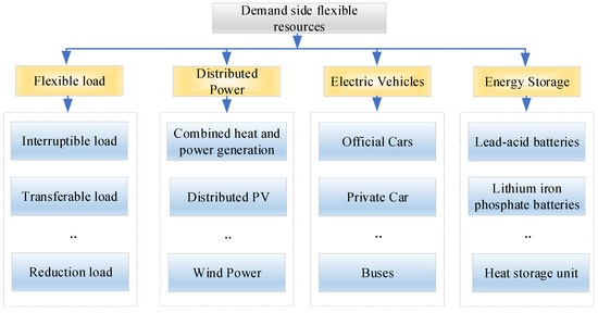
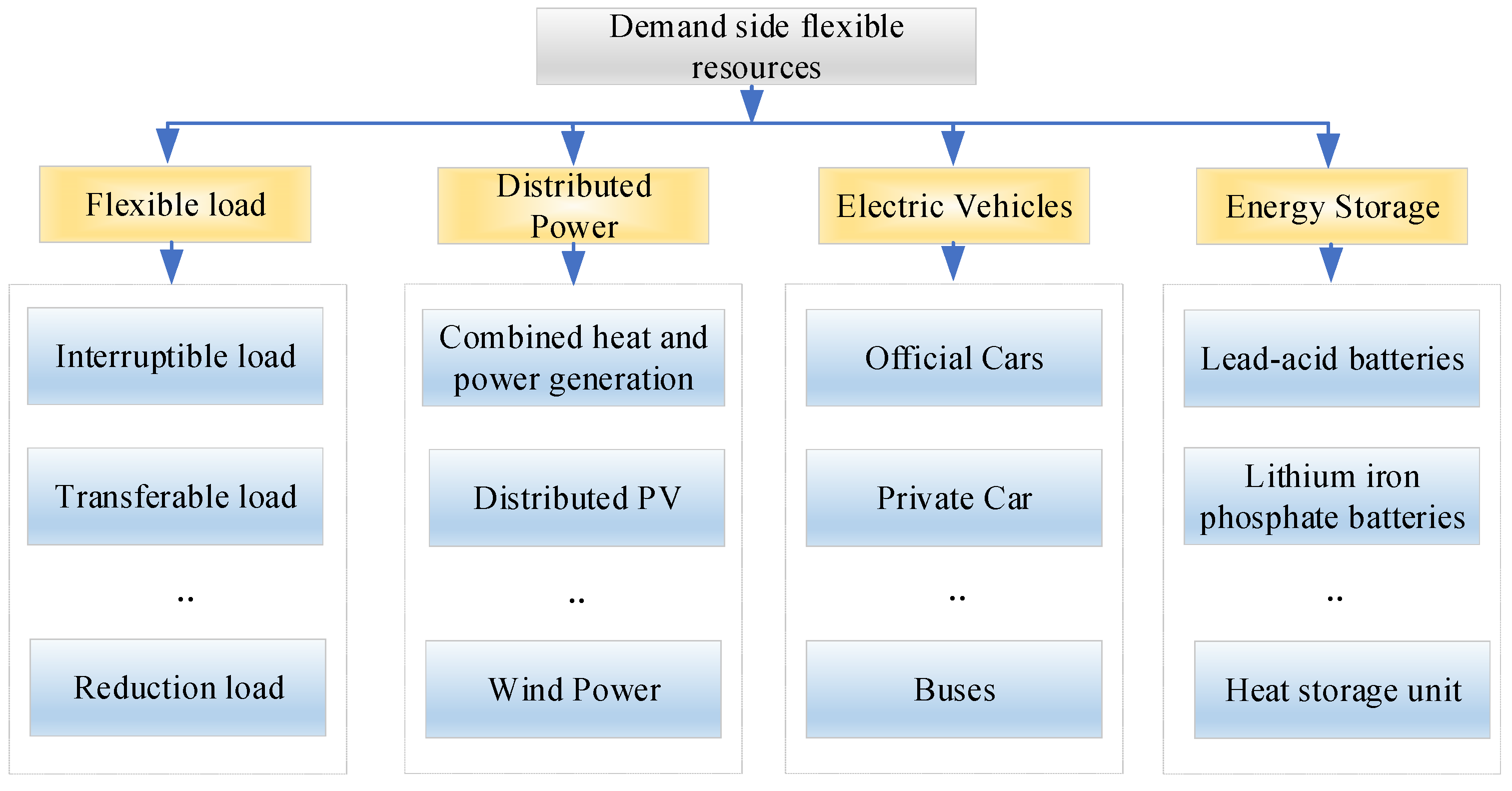
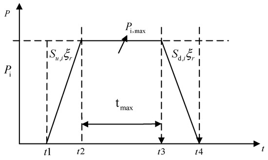
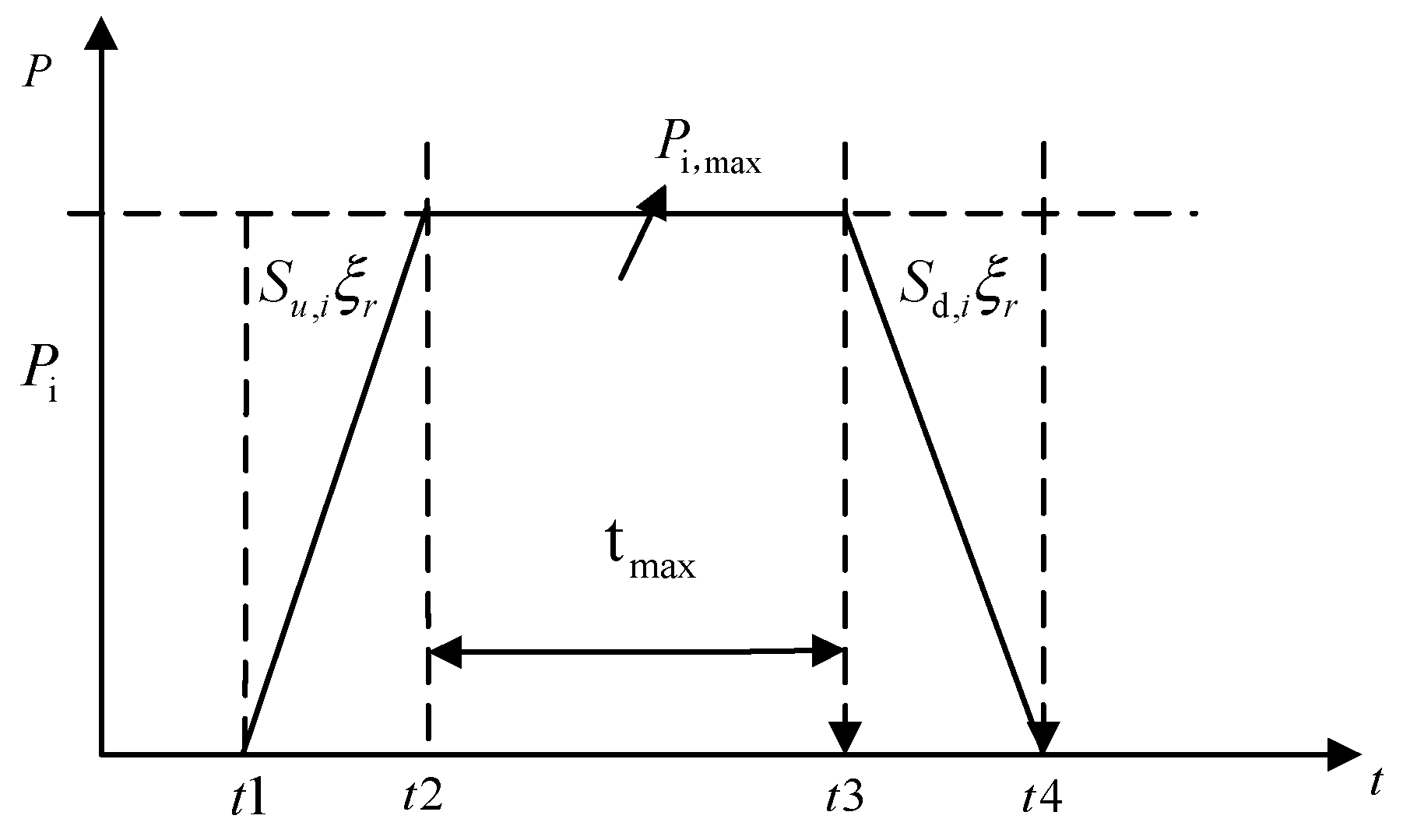
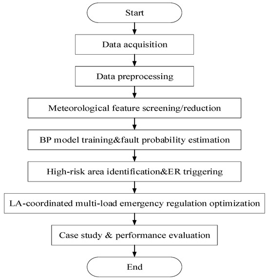
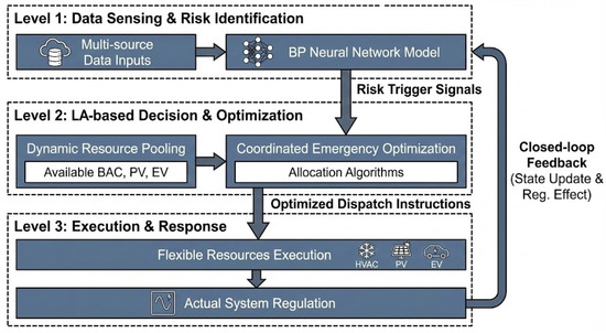
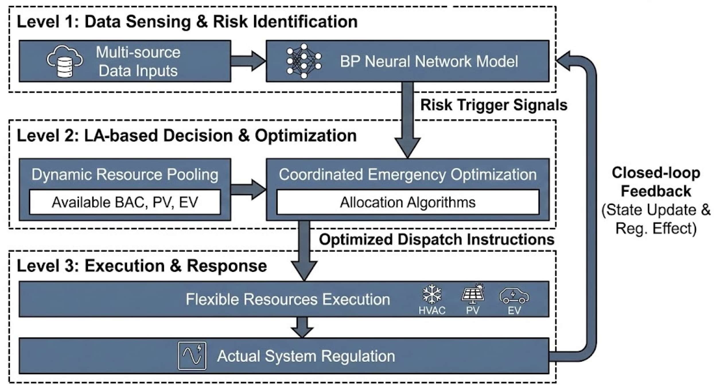
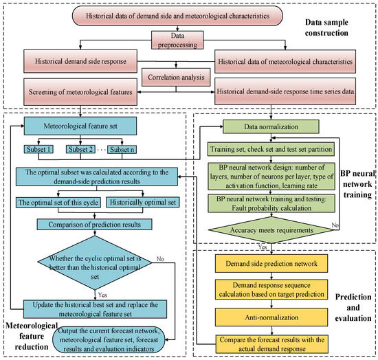
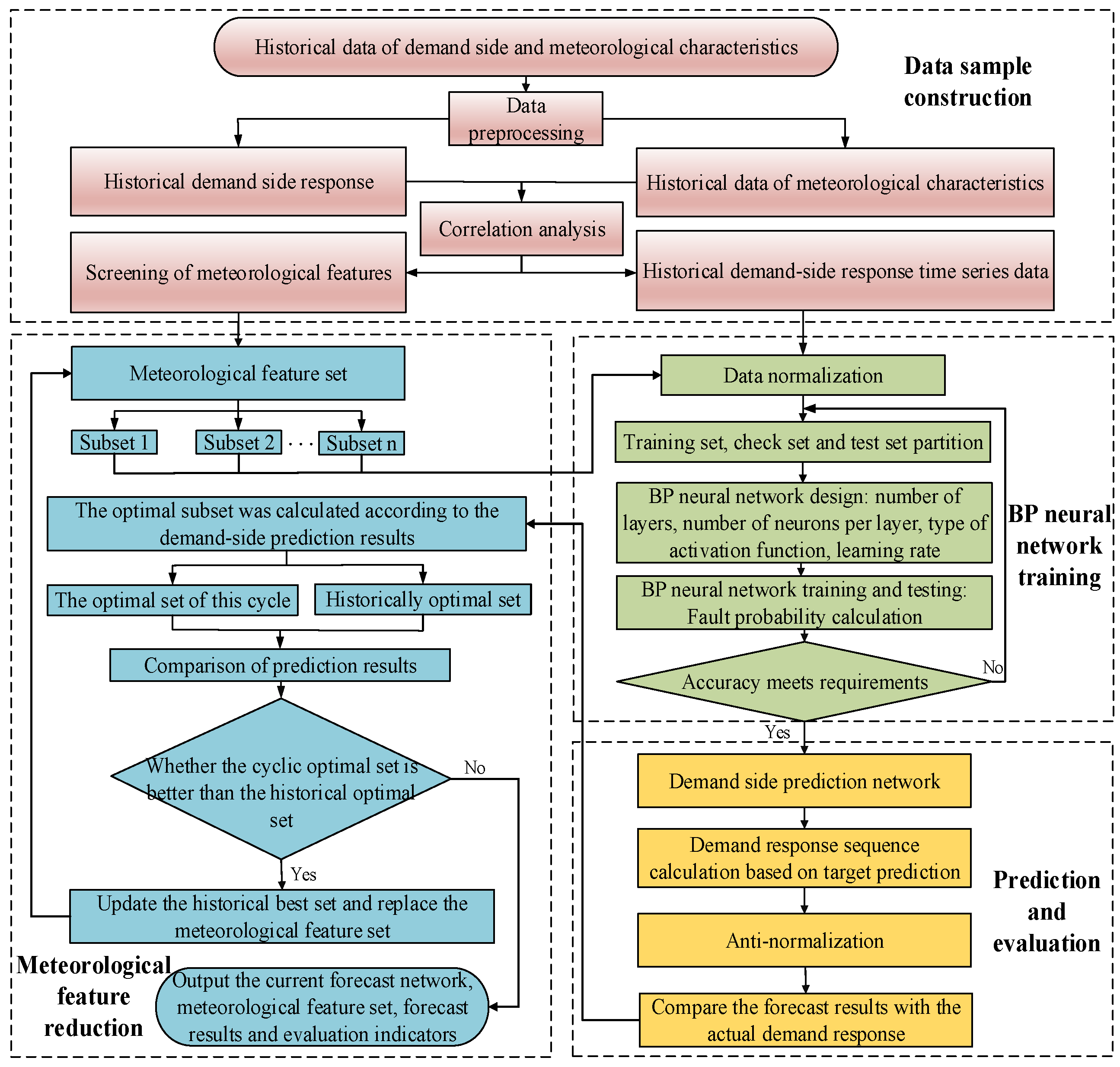
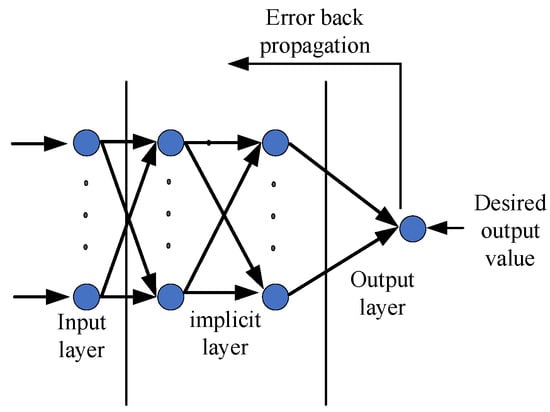
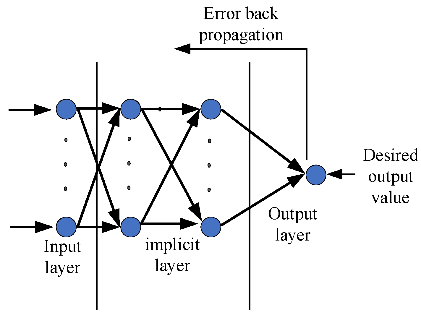
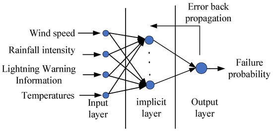
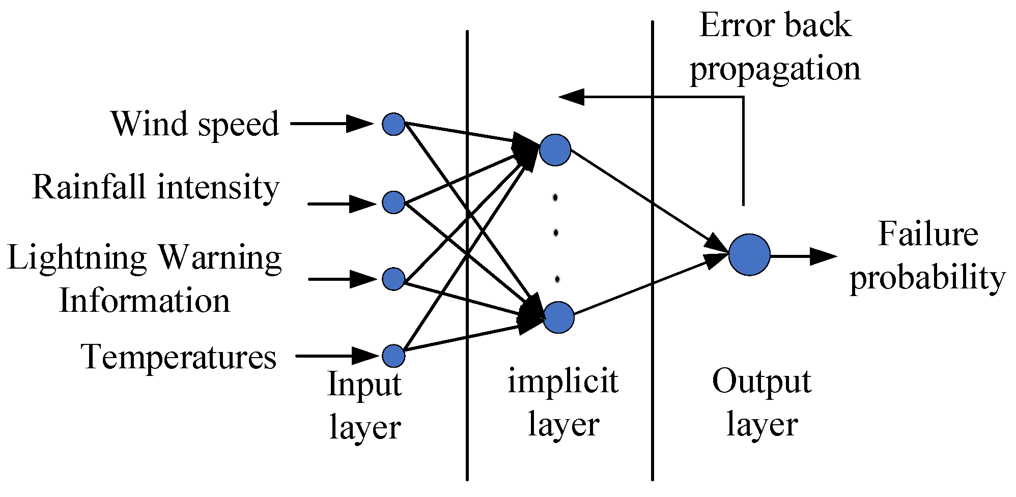
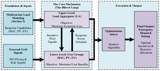
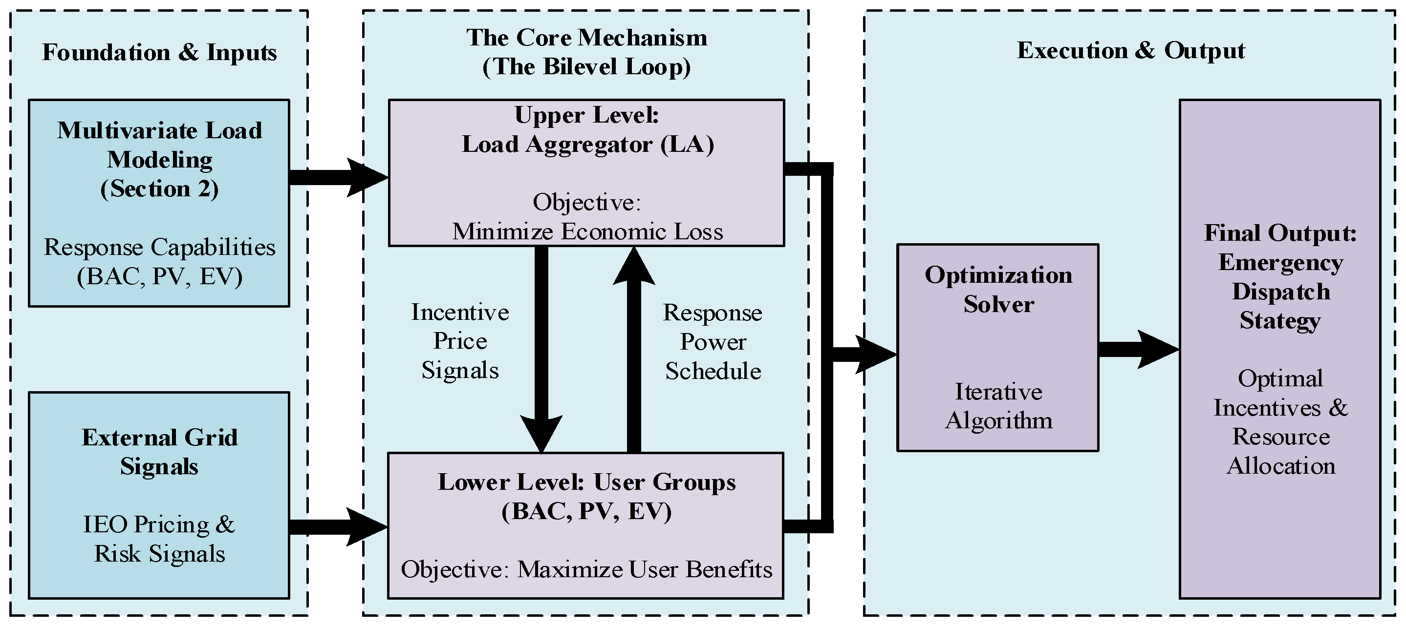
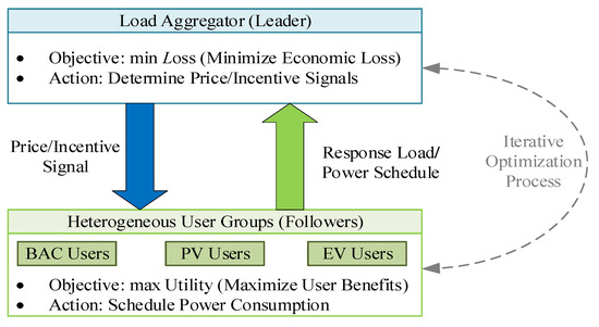
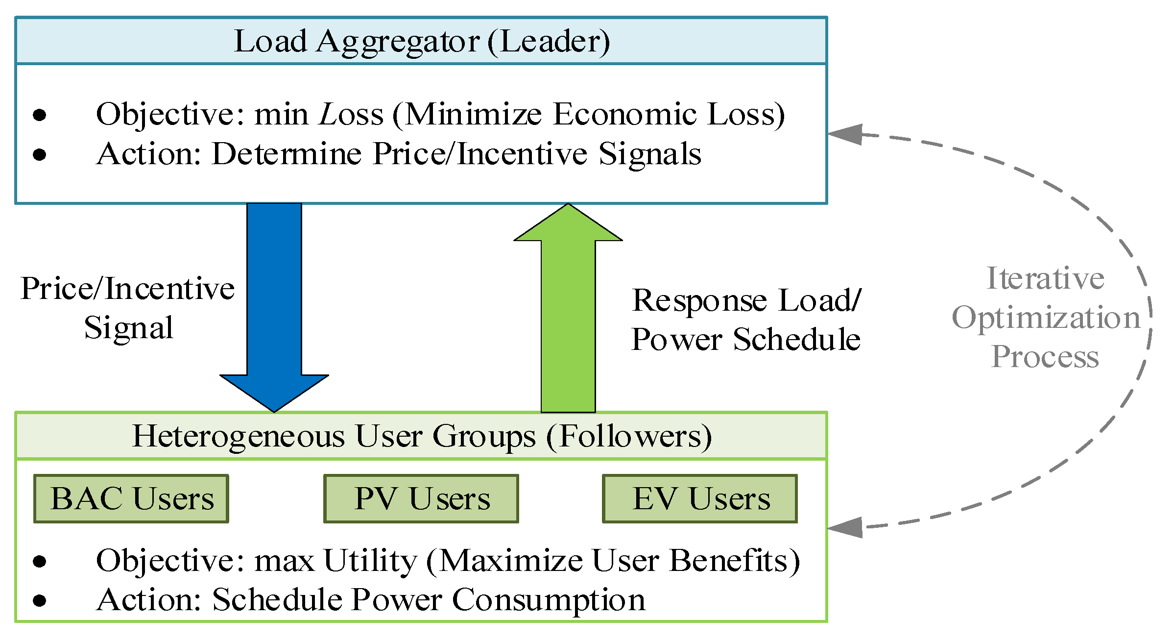
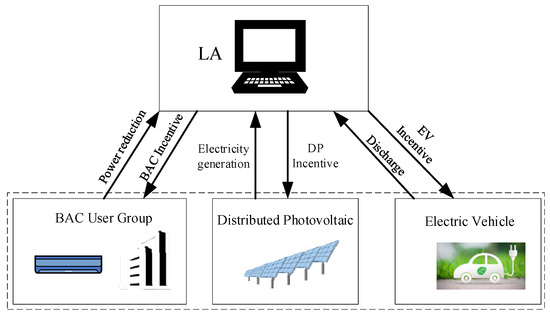
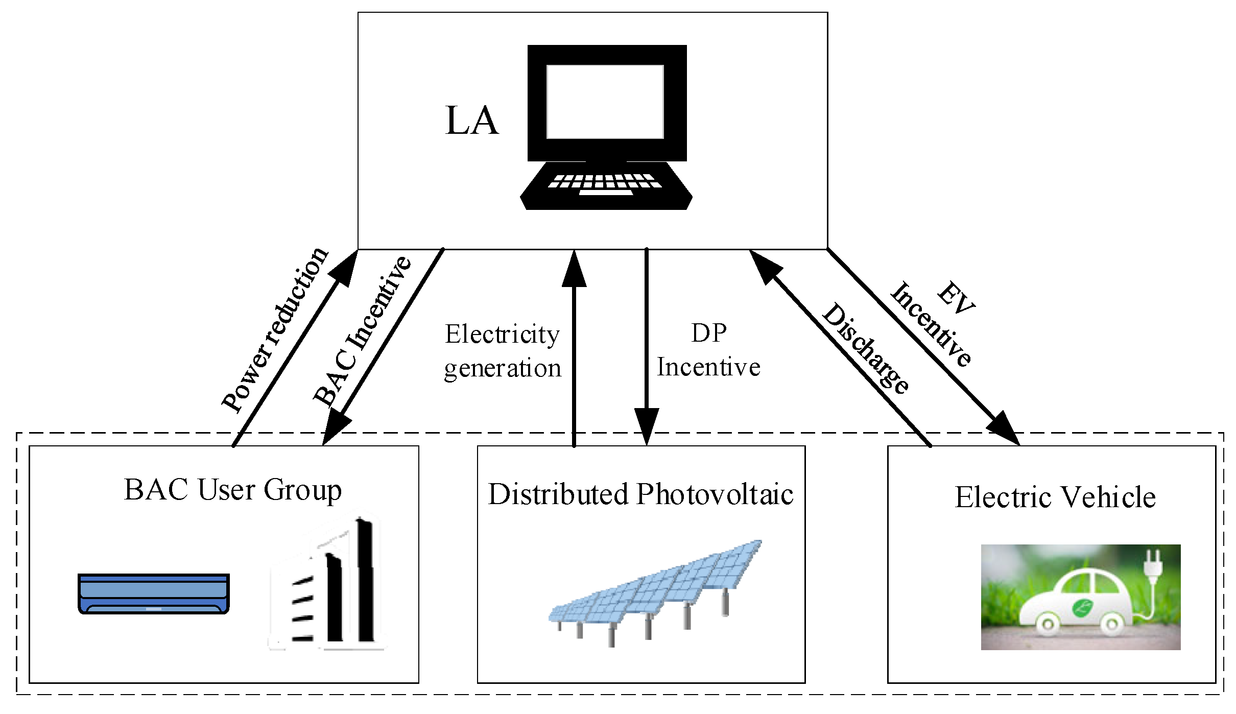
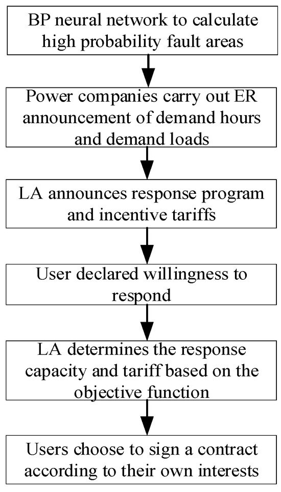
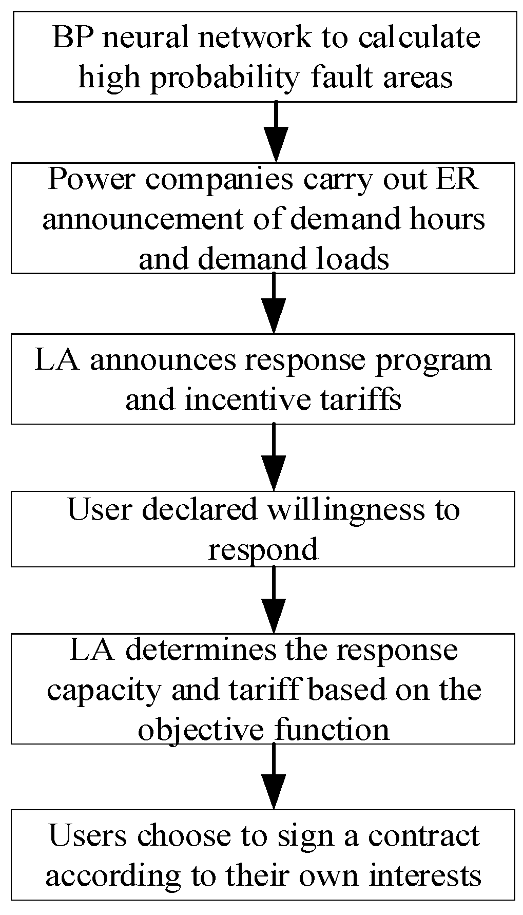
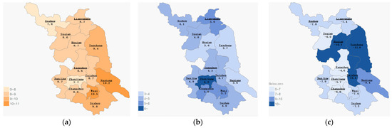
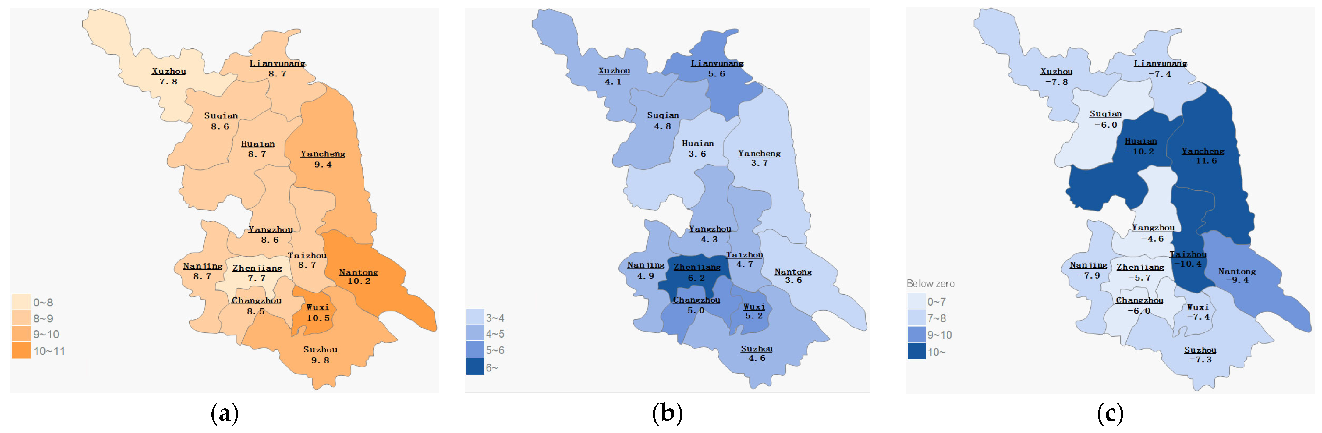
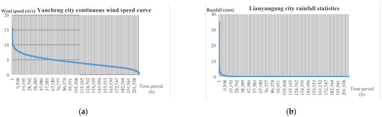
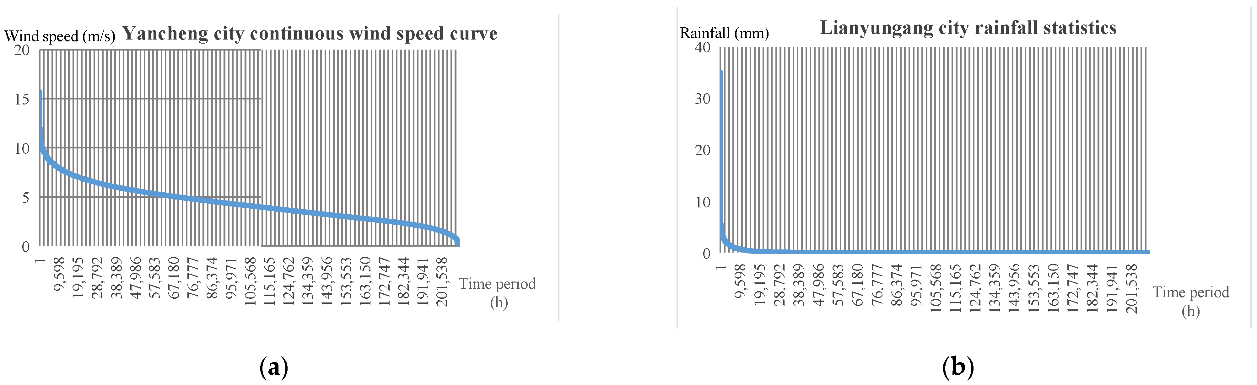
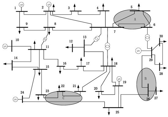
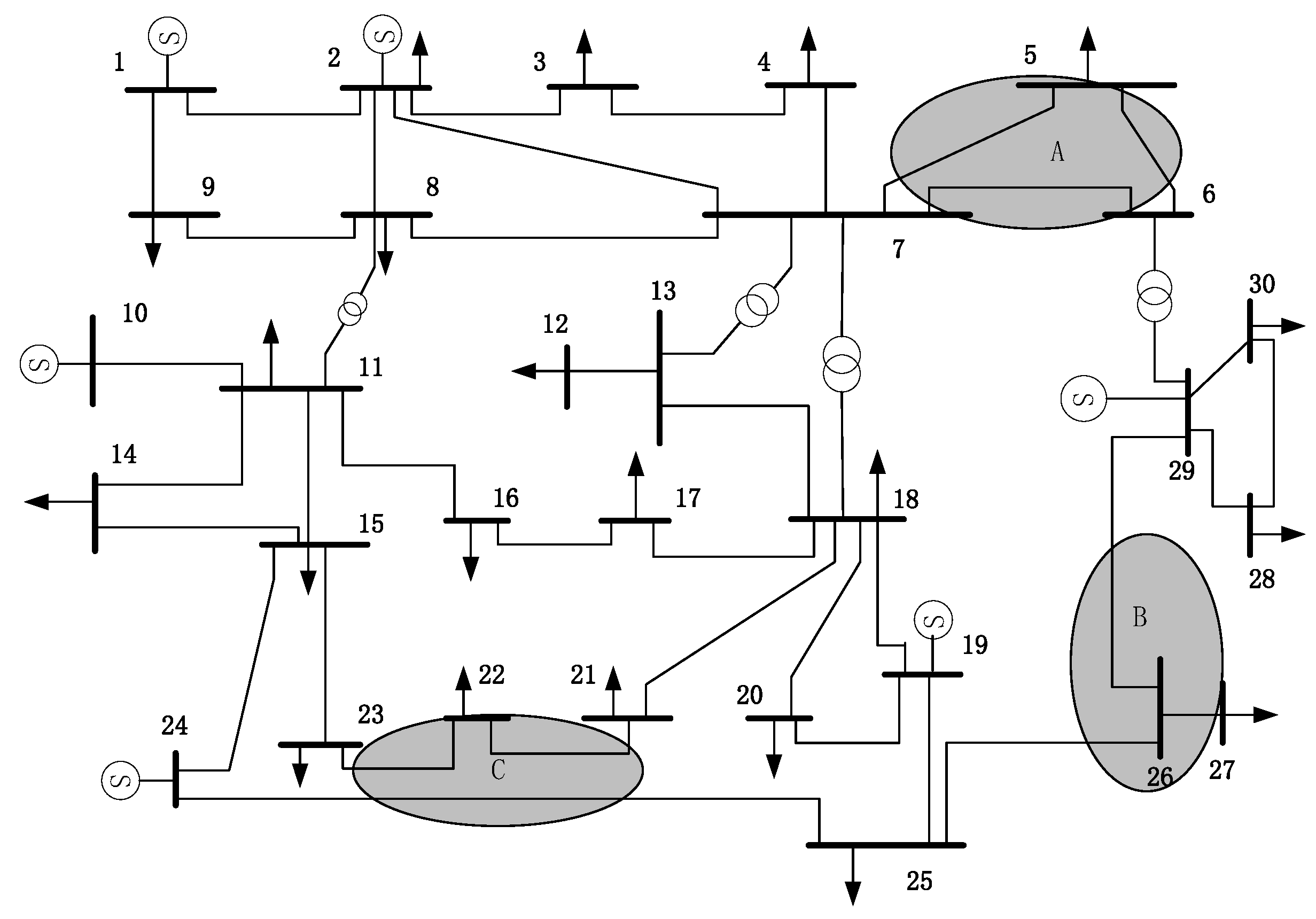
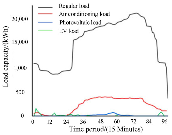
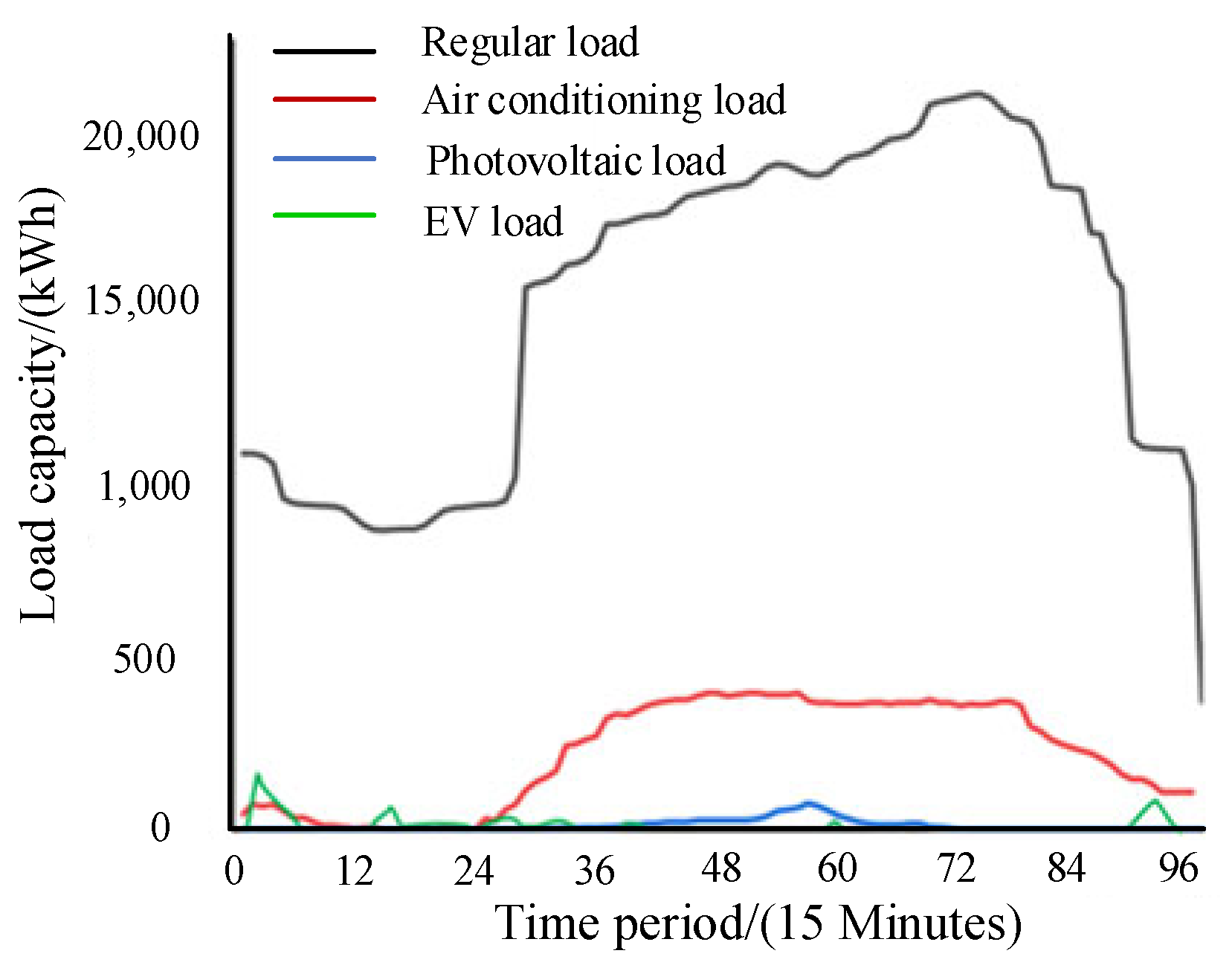
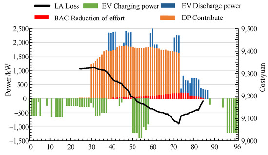
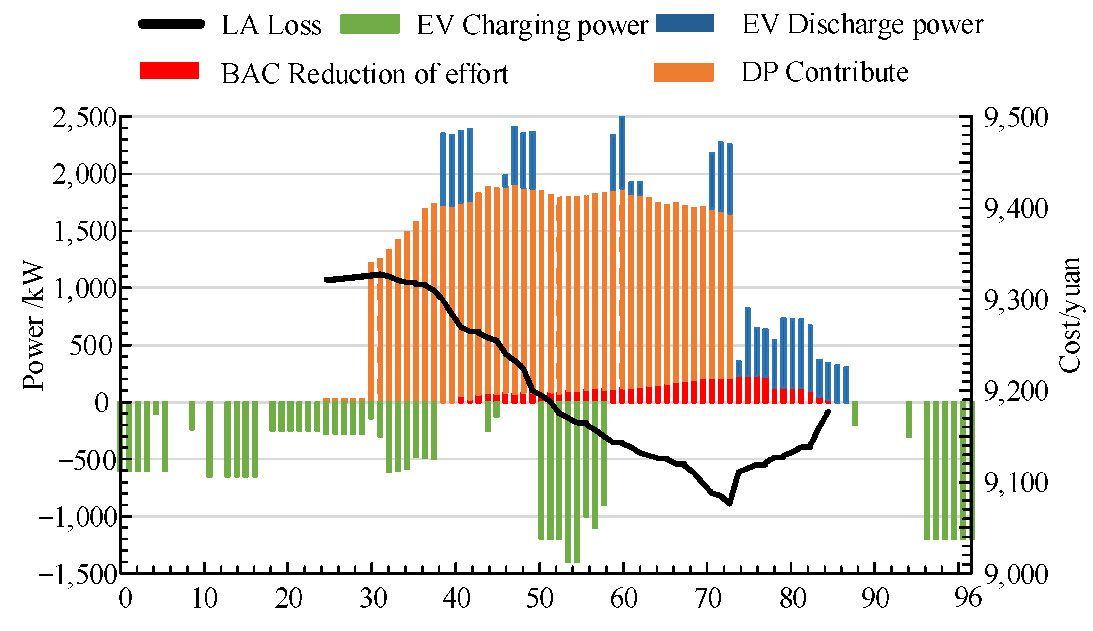

Disclaimer/Publisher’s Note: The statements, opinions and data contained in all publications are solely those of the individual author(s) and contributor(s) and not of MDPI and/or the editor(s). MDPI and/or the editor(s) disclaim responsibility for any injury to people or property resulting from any ideas, methods, instructions or products referred to in the content. |
© 2026 by the authors. Licensee MDPI, Basel, Switzerland. This article is an open access article distributed under the terms and conditions of the Creative Commons Attribution (CC BY) license.