Modeling Yarn Structural Heterogeneity via Generalized Poisson and Gamma Mixture Distributions

Abstract

This study investigates the applicability of finite mixture models (FMMs) for accurately modeling yarn structural quality parameters in 28/1 Ne ring-spun polyester/viscose yarns, focusing on yarn hairiness and twist. The research addresses the need for advanced statistical modeling techniques to better capture the inherent heterogeneity in textile production data. To this end, the Poisson mixture model is employed to represent the twist parameter, while the gamma mixture model is used to model the continuous hairiness indices (S3 CV% and H). Model parameters are estimated using the expectation–maximization (EM) algorithm, and model selection is guided by the Akaike and Bayesian information criteria (AIC and BIC). The results reveal that a two-component mixture distribution provides the optimal fit varies by parameter: twist is best represented by a two-component generalized Poisson mixture, which preserves the integer support of the measurements while relaxing the equidispersion restriction of the ordinary Poisson distribution, whereas hairiness (S3 CV%, H) is best described by two- and three-component gamma mixture distributions, respectively. Model adequacy is assessed by a parametric bootstrap with re-estimation on each replicate. The two-component gamma mixture for S3 CV% is not rejected, whereas residual departures remain for H and, more substantially, for twist, where the concentration of the variable on six recorded levels limits the adequacy of any continuous or semi-continuous specification. These findings highlight the robustness of FMMs in capturing complex distributional patterns in yarn data, extending previous work on yarn imperfections and mechanical properties, and demonstrating their potential in enhancing quality assessment and process control in the textile industry.

1. Introduction

Many real-world datasets exhibit complex structures because observations may originate from multiple underlying sources of variation. Traditional statistical models typically assume that all observations are generated from a single probability distribution. However, this assumption may not always hold in practice, since observed data may arise from several latent subpopulations whose identities are unknown. When such heterogeneity exists, single-distribution models may fail to represent the true structure of the data adequately. In these situations, finite mixture models (FMMs) provide a flexible statistical framework for modeling heterogeneous datasets [1].

Finite mixture models describe the overall probability distribution of a dataset as a weighted combination of several component distributions, where each component represents a latent subgroup within the population. This approach enables researchers to capture complex distributional shapes, such as multimodal or skewed distributions, and identify hidden structures within the data. Because of their flexibility and strong theoretical foundations, finite mixture models have been successfully applied in various research fields. For example, they are widely used in clustering and model-based classification problems [2], reliability and failure-time analysis [3], and transportation safety studies for modeling crash frequency data and capturing unobserved heterogeneity [4].

Also, in many engineering and manufacturing processes, data is generated by complex systems in which several factors simultaneously affect the observed outcomes. In the textile literature, the application of finite mixture models has primarily focused on characterizing cotton fiber length distributions. In this context, the use of two-component Weibull mixture distributions has been shown to be an effective approach for describing fiber length characteristics [5]. Subsequent studies further confirmed the effectiveness of this modeling framework by employing two-component Weibull mixture models to represent fiber length distributions obtained from experimental measurements [6,7]. Later research extended the finite mixture modeling approach by incorporating additional probability distributions, such as the normal and power distributions, thereby enabling the development of probability density functions for both carded and combed cotton fibers based on parameters derived from fiber length measurements [8]. The use of finite mixture models to characterize cotton fiber length distributions has also been discussed by Kuang et al. [9]. By examining fiber length histograms, researchers have constructed parametric continuous models using mixtures of Weibull distributions. This modeling strategy has been applied to cotton fiber samples from various spinning stages—including bale, card mat, carded sliver, combed sliver, and finished sliver—to accurately represent fiber length distributions. Beyond fiber length modeling, finite mixture models have been applied to yarn quality analysis, modeling yarn imperfections. The findings of that study demonstrated that mixture distributions can effectively capture the heterogeneous nature of yarn quality data and provide improved statistical representations compared to traditional single-distribution models [10].

Alongside these studies in probabilistic modeling, recent advances in artificial intelligence and data-driven methods have considerably broadened the methodological landscape of yarn quality analysis. Machine learning and deep learning techniques, including artificial neural networks (ANNs), convolutional neural networks (CNNs), and YOLO-based architectures, have been applied to the prediction and characterization of yarn properties and defects. Duo et al. [11] employed artificial neural network (ANN) and multiple linear regression (MLR) models using online yarn-quality data collected by an electronic yarn clearer during the winding process to predict offline coefficient of variation (CV) and hairiness values of cotton yarns, with the ANN model providing higher prediction accuracy and showing potential for real-time quality monitoring. Abd-Elhamied et al. [12] combined image processing with artificial neural networks to estimate tenacity, elongation, coefficient of mass variation, and yarn imperfections in ring-spun and compact cotton yarns. More recently, Pereira et al. [13] applied an enhanced YOLOv5s6-based deep learning approach to yarn hairiness characterization, enabling the detection and distinction of protruding and loop fibers in digital yarn images. Xu et al. [14] proposed a complementary knowledge-augmented multimodal learning method for yarn-quality soft sensing, combining fiber properties and process parameters with yarn appearance images to improve the estimation of yarn quality indices. Collectively, these studies demonstrate the increasing use of data-driven and AI-based methods for the prediction, estimation, and characterization of yarn quality attributes.

While these data-driven approaches are particularly valuable for prediction and classification, they generally rely on predefined labels or specified input–output relationships. In industrial practice, however, historical production datasets are not always accompanied by predefined quality labels or detailed process covariates linked to individual observations. Under such conditions, FMMs provide a complementary unsupervised probabilistic approach by identifying latent subpopulations directly from observed quality measurements without requiring predefined class labels. This capability makes FMMs particularly useful for characterizing hidden heterogeneity in real-world production data when detailed labeled or process-linked information is unavailable.

In the present study, FMMs were therefore employed to explore the underlying distributional structure of twist and hairiness measurements obtained from real industrial production records. This approach enables the identification of latent subpopulations and provides a probabilistic characterization of heterogeneity that a single-distribution model may not adequately represent. Such information can provide a more detailed understanding of variability in yarn quality parameters and may contribute to the identification of atypical patterns relevant to quality monitoring. Although the present study builds on the FMM framework used in the companion study [10], it addresses a different class of yarn quality parameters, namely twist and hairiness. Unlike yarn imperfections, twist and hairiness represent distinct structural characteristics of yarn and exhibit parameter-specific distributional patterns. Their analysis therefore extends the application of FMMs to a different quality domain, enabling the identification and probabilistic characterization of latent structures specifically associated with yarn twist and surface hairiness. Accordingly, the objective of this study is to investigate the applicability of finite mixture models for modeling the structural characteristics of 28/1 Ne ring-spun polyester/viscose yarns, with a particular focus on hairiness (expressed through the S3 CV% and H indices) and twist (t/m), which are key parameters influencing downstream weaving and knitting performance as well as fabric appearance.

Yarn hairiness, which represents the presence of fibre ends and loops protruding from the yarn body, plays a critical role in both processing efficiency and final product quality; excessive hairiness can lead to yarn breakages, reduced machine efficiency, poor surface appearance, and increased pilling tendency [15]. While the S3 index quantifies the number of hairs exceeding 3 mm in length per unit length of yarn, the H index provides a complementary measure of overall hairiness by representing the equivalent cylindrical surface formed by protruding fibres; together, these two indices are commonly used to characterize different aspects of yarn hairiness [15]. Yarn twist, which provides cohesion by binding fibres together, is a fundamental structural parameter governing yarn strength, durability, and overall performance; although an optimal level of twist improves fibre cohesion, excessive twist may lead to fibre misalignment and deterioration in mechanical properties [16,17].

Understanding the probability distributions of these parameters is therefore essential for predicting yarn behaviour, enabling proactive quality control, and optimizing spinning process settings. Building on the FMM framework previously validated for yarn imperfections and mechanical properties in ring-spun polyester/viscose yarns [10], this study extends the approach to hairiness and twist, employing generalized Poisson mixture distributions for the twist parameter and gamma mixture distributions.

The remainder of this paper is organized as follows: Section 2 presents the materials and methods, including the data collection procedure and the theoretical background of the Poisson and gamma mixture models; Section 3 presents and discusses the results of the analysis; and Section 4 concludes the study by summarizing the main findings and their implications for the textile industry.

2. Materials and Methods

2.1. Data Sets

The data used in this study were obtained from an anonymized textile manufacturer in Türkiye, previously described in our companion study on yarn imperfections [10] and were obtained from a 28/1 Ne ring-spun, combed (RNG COM) polyester/viscose (PE/V) yarn with a composition ratio of 65/35. The dataset consists of 769 quality-control test results, collected between January 2019 and April 2022.

Twist and hairiness were monitored as part of the manufacturer’s routine yarn quality-control protocol. For both parameters, 16 cops were sampled at 120 yards from each ring, with testing performed once a day and additionally whenever a new yarn type was introduced (i.e., once per machine per day). Twist was measured using a Zweigle D315 twist tester (Zweigle GmbH & Co. KG, Reutlingen, Germany), while hairiness (S3 and H indices) was measured using a Zweigle G567 hairiness tester (Zweigle GmbH & Co. KG, Reutlingen, Germany). Each twist record corresponds to a single integer-valued turn-count measurement obtained from an individual quality-control test using the untwist–retwist counting method. Accordingly, the twist observations included in the statistical analysis are integer-valued measurements expressed in turns per meter (t/m). The reference to the introduction of a new yarn type reflects the manufacturer’s facility-wide quality-control protocol, which covers multiple yarn types produced on different machines. The 769 records analyzed in the present study were filtered from the manufacturer’s full quality-control database to include exclusively the 28/1 Ne ring-spun, combed PE/V (65/35) yarn construction. Thus, all observations included in the present analysis correspond to the same yarn construction.

2.2. A Unified Estimation Framework for the Two Mixture Families Considered

Finite mixture models (FMMs) provide a flexible statistical tool for representing populations composed of several latent subgroups, particularly suitable when a dataset is known to originate from a mixture of underlying distributions whose individual forms are not directly observable [18,19]. This mixture structure allows the EM estimation equations for both families to be derived from a single, unified likelihood-augmentation argument, rather than being re-derived independently for each family as is customary in the classical mixture-modeling literature.

Let x₁,…,x_n denote n independent observations of a given quality parameter, assumed to arise from a K-component mixture

$$f\left(x_i;\mathsf{\Psi }\right)={\displaystyle {\sum }_{k=1}^K}{\pi }_{k}f\left(x_i;{\eta }_k\right),{\sum }_k{\pi }_k=1,{\pi }_k\ge 0$$

(1)

where Ψ collects all mixing weights π = (π₁,…,π_k) and component-specific parameters η = (η₁, …, η_k), and each component density f(·;η_k) belongs to an exponential family, i.e., can be written as [20]

$$f\left(x;{\eta }_k\right)=\exp \left\{{\eta }_k^{T}T\left(x\right)-A\left({\eta }_k\right)+c\left(x\right)\right\}$$

(2)

for some natural parameter η_k, sufficient statistic T(x), log-partition function A(η_k), and base measure c(x). Equation (2) is not restrictive here: setting η_k = logλ_k, T(x) = x, A(η_k) = eη_k, c(x) = −log(x!) recovers the Poisson component used for twist, while setting η_k = (α_k,β_k) with a suitable reparameterization recovers the gamma component used for hairiness.

Because component membership is unobserved, we introduce, for each observation i, a latent indicator vector z_i = (z_i1,…,z_ik) with z_ik = 1 if x_i was generated by component k and 0 otherwise, and z_i ~ Categorical(π). The complete-data log-likelihood, treating (x_i,z_i1) jointly, is

$${\mathcal{l}}_c\left(\mathsf{\Psi }\right)={\displaystyle {\sum }_{i=1}^n}{\displaystyle {\sum }_{k=1}^K}{z}_{\mathit{ik}}\left[{\log \pi }_k+{\eta }_k^{T}T\left(x_i\right)-A\left({\eta }_k\right)+c\left(x_i\right)\right]$$

(3)

E-step: At iteration r, given current estimates Ψ^(r), the conditional expectation of z_ik, the responsibility of component k for observation i, is obtained by Bayes’ rule:

$$r_{\mathit{ik}}^{\left(r\right)}={\displaystyle \frac{{\pi }_k^{\left(r\right)}f\left(x_i;{\eta }_k^{\left(r\right)}\right)}{{\displaystyle {\sum }_{j=1}^K}{\pi }_j^{\left(r\right)}f\left(x_i;{\eta }_j^{\left(r\right)}\right)}}$$

(4)

Because Equation (3) is linear in z_ik, taking its expectation under the posterior of Equation (4) simply replaces each z_ik by r_ik^(r), giving the expected complete-data log-likelihood

$$Q\left(\mathsf{\Psi }|{\mathsf{\Psi }}^{\left(r\right)}\right)={\displaystyle {\sum }_{i=1}^n}{\displaystyle {\sum }_{k=1}^K}{r}_{\mathit{ik}}^{\left(r\right)}\left[{\log \pi }_k+{\eta }_k^{T}T\left(x_i\right)-A\left({\eta }_k\right)+c\left(x_i\right)\right]$$

(5)

M-step: Q is maximized over π subject to Σπ_k= 1, and separately over each η_k. The constrained maximization over π (via a Lagrange multiplier) always yields the same closed-form update regardless of the component family:

$${\pi }_k^{\left(r+1\right)}={\displaystyle \frac{1}{n}}{\displaystyle {\sum }_{i=1}^n}{r}_{\mathit{ik}}^{\left(r\right)}$$

(6)

The maximization over η_k reduces, for any exponential-family component, to match the expected sufficient statistic:

$${\displaystyle \frac{\partial A\left({\eta }_k\right)}{\partial {\eta }_k}}={\displaystyle \frac{{\displaystyle {\sum }_{i=1}^n}{r}_{\mathit{ik}}^{\left(r\right)}T\left(x_i\right)}{{\displaystyle {\sum }_{i=1}^n}{r}_{\mathit{ik}}^{\left(r\right)}}}$$

(7)

which has a closed-form solution when A(·) is invertible in closed form and requires an additional numerical step when it is not. Equations (4), (6) and (7) are iterated until the observed-data log-likelihood

$$\mathcal{l}\left(\mathsf{\Psi }\right)={\displaystyle {\sum }_{i=1}^n}\log \left({\displaystyle {\sum }_{k=1}^K}{\pi }_{k}f\left(x_i;{\eta }_k\right))\right)$$

(8)

increases by less than a fixed tolerance between successive iterations; the EM algorithm guarantees 𝓁(Ψ^(r+1)) ≥ 𝓁(Ψ^(r)) at every step [18,19].

Two general remarks apply to both instantiations below. First, the mixture likelihood in Equation (8) is invariant to any permutation of the component labels 1,…,K; we resolve this by re-ordering components in ascending order of their component-specific mean after convergence, for every model and every restart [21]. Second, because Equation (8) is generally multimodal in Ψ, EM converges only to a local maximum; this is our multi-start strategy for mitigating [22].

2.3. Instantiation for Count Data: The Poisson Mixture Distribution

For the twist parameter, whose measurement resolution produces discrete, count-like observations, we set f(x;η_k) to the Poisson probability mass function

$$f\left(x;{\lambda }_k\right)={\displaystyle \frac{{\lambda }_k^x{e}^{-{\lambda }_k}}{x!}},\hspace{1em}x=0,1,2,\dots ,\hspace{1em}k=1,\dots ,K$$

(9)

corresponding to natural parameter η_k = logλ_k, sufficient statistic T(x) = x, and log-partition A(η_k) = eη_k= λ_k. The responsibility of Equation (4) becomes

$$r_{\mathit{ik}}^{\left(r\right)}={\displaystyle \frac{{\pi }_k^{\left(r\right)}{\left({\lambda }_k^{\left(r\right)}\right)}^{x_i}{e}^{-{\lambda }_k^{\left(r\right)}}}{{\displaystyle {\sum }_{j=1}^K}{\pi }_j^{\left(r\right)}{\left({\lambda }_j^{\left(r\right)}\right)}^{x_i}{e}^{-{\lambda }_j^{\left(r\right)}}}}$$

(10)

and, since ∂A/∂η_k= eη_k = λ_k, Equation (7) is invertible in closed form, giving the well-known update

$${\lambda }_k^{\left(r+1\right)}={\displaystyle \frac{{\displaystyle {\sum }_{i=1}^n}{r}_{\mathit{ik}}^{\left(r\right)}{x}_i}{{\displaystyle {\sum }_{i=1}^n}{r}_{\mathit{ik}}^{\left(r\right)}}}$$

(11)

so that a single pass of Equations (6), (10) and (11) constitutes one EM iteration for the twist model. Because a Poisson random variable satisfies Var(X|λ_k) = E(X|λ_k) = λ_k, the law of total expectation and variance give the marginal mean and variance of the fitted mixture as

$${\mu }_{\mathrm{twist}}={\displaystyle {\sum }_{k=1}^K}{\pi }_k{\lambda }_k$$

(12)

$${\sigma }_{\mathrm{twist}}^2={\displaystyle {\sum }_{k=1}^K}{\pi }_k\left({\lambda }_k+{\lambda }_k^2\right)-{\mu }_{\mathrm{twist}}^2$$

(13)

The ordinary Poisson distribution constrains the conditional variance to equal the conditional mean. When this restriction is not supported by the data, a distribution that preserves integer support while allowing the variance to differ from the mean is required. We therefore also consider the generalized Poisson distribution, whose probability mass function is P(X = x) = θ(θ + λx)^(x−1)e^{(−θ−λx)}/x!,x = 0,1,2,… with θ > 0 and λ < 1. Its mean and variance are E(X) = θ/(1 − λ) and Var(X) = θ/(1 − λ)³, so the dispersion index equals (1 − λ)⁽⁻²⁾. The ordinary Poisson distribution is recovered when λ = 0. Negative values of λ produce underdispersion and positive values produce overdispersion, so this family nests the Poisson specification and permits a direct assessment of the equidispersion restriction. For λ < 0 the support is truncated at the largest integer m satisfying θ + λm > 0, and we verified numerically that the fitted component probabilities sum to unity to within 10⁻⁶ over this support.

A K-component generalized Poisson mixture has density f(x) = Σw_kGP(x;θ_k,λ_k) with Σw_k = 1 and w_k > 0. Since the M-step for θ_k and λ_k does not admit a closed-form solution, this mixture is estimated by direct numerical maximization of the observed-data log-likelihood. In estimation, λ was restricted to the interval from −3 to 0, the mixing proportions to values of at least 0.02, and the component means to the range spanned by the observed data, in order to exclude degenerate solutions in which a component collapses onto a single support point.

2.4. Instantiation for Continuous, Right-Skewed Data: The Gamma Mixture Distribution

For hairiness (S3 CV%, H); strictly positive, continuous, right-skewed measurements; we set f(x;η_k) to the gamma density parameterized by shape α_k and rate β_k:

$$f\left(x;{\alpha }_k,{\beta }_k\right)={\displaystyle \frac{{\beta }_k^{{\alpha }_k}{x}^{{\alpha }_k-1}{e}^{-{\beta }_{k}x}}{\mathsf{\Gamma }\left({\alpha }_k\right)}},x>0$$

(14)

Unlike the Poisson case, the gamma density has two component-specific parameters (α_k,β_k), so the sufficient-statistic-matching step of Equation (7) must be solved jointly for both. The responsibility update follows directly from Equation (4):

$$r_{\mathit{ik}}^{\left(r\right)}={\displaystyle \frac{{\pi }_k^{\left(r\right)}f\left(x_i;{\alpha }_k^{\left(r\right)},{\beta }_k^{\left(r\right)}\right)}{{\displaystyle {\sum }_{j=1}^K}{\pi }_j^{\left(r\right)}f\left(x_i;{\alpha }_j^{\left(r\right)},{\beta }_j^{\left(r\right)}\right)}}$$

(15)

Writing out Q for the gamma family and differentiating with respect to β_k gives a closed-form expression for the rate in terms of the shape. Because the shape is updated first, as described below, the updated value ${\alpha }_k^{\left(r+1\right)}$ enters this expression:

$${\beta }_k^{\left(r+1\right)}={\displaystyle \frac{{\alpha }_k^{\left(r+1\right)}{\displaystyle {\sum }_{i=1}^n}{r}_{\mathit{ik}}^{\left(r\right)}}{{\displaystyle {\sum }_{i=1}^n}{r}_{\mathit{ik}}^{\left(r\right)}{x}_i}}$$

(16)

By contrast, differentiating Q with respect to α_k produces a transcendental equation involving the digamma function ψ(·)=Γ′(·)/Γ(·). The shape parameter of each gamma component is updated by solving the profiled score equation log(α_k) − ψ(α_k) = s_k numerically to machine precision. This root is the exact maximizer of the expected complete-data log-likelihood with respect to α_k, and the rate parameter is then obtained in closed form from the updated shape. The M-step therefore attains the maximum of the Q-function at each iteration, so the procedure is an ordinary EM algorithm implemented with a numerical M-step rather than a generalized EM algorithm, and the standard monotonicity guarantee applies. We verified numerically that the observed-data log-likelihood is non-decreasing across iterations for every reported fit.

$$\log \left({\alpha }_k\right)-\psi \left({\alpha }_k\right)=\log \left({\overline{x}}_k\right)-{\displaystyle \frac{\sum _i{r}_{\mathit{ik}}^{\left(r\right)}{\log x}_i}{\sum _i{r}_{\mathit{ik}}^{\left(r\right)}}}\equiv s_k,{\overline{x}}_k={\displaystyle \frac{\sum _i{r}_{\mathit{ik}}^{\left(r\right)}{x}_i}{\sum _i{r}_{\mathit{ik}}^{\left(r\right)}}}$$

(17)

which has no closed-form solution because ψ(·) is transcendental [23]. We solve Equation (17) at each EM iteration using Newton’s method, initialized from Minka’s moment-based approximation ${\hat{\alpha }}_0=\left(3-s_k+\sqrt{{\left(s_k-3\right)}^2+24s_k}\right)/\left(12s_k\right)$, and refined by the update [24,25]

$${\alpha }_k^{\left(t+1\right)}={\alpha }_k^{\left(t\right)}-{\displaystyle \frac{\log \left({\alpha }_k^{\left(t\right)}\right)-\psi \left({\alpha }_k^{\left(t\right)}\right)-s_k}{\frac{1}{{\alpha }_k^{\left(t\right)}}-{\mathit{\psi }}^{\prime }\left({\alpha }_k^{\left(t\right)}\right)}}$$

(18)

iterated to convergence, where ψ′(·) is the trigamma function [26,27]. This inner Newton loop, nested inside the outer EM loop, together with Equations (15) and (16), constitutes one EM iteration for each gamma-distributed parameter.

Given the fitted parameters, the mixture mean and variance for hairiness follow, again via the law of total expectation/variance and the gamma moments $\mathrm{Var}\left(X|{\alpha }_k,{\beta }_k\right)={\alpha }_k/{\beta }_k^2$:

$${\mu }_{\mathrm{mix}}={\displaystyle {\sum }_{k=1}^K}{\pi }_k{\displaystyle \frac{{\alpha }_k}{{\beta }_k}}$$

(19)

$${\sigma }_{\mathrm{mix}}^2={\displaystyle {\sum }_{k=1}^K}{\pi }_k\left({\displaystyle \frac{{\alpha }_k}{{\beta }_k^2}}+{\displaystyle \frac{{\alpha }_k^2}{{\beta }_k^2}}\right)-{\mu }_{\mathrm{mix}}^2$$

(20)

2.5. Model Order Selection, Initialization, and Convergence

For each of the three parameters, models with K = 1, 2, 3, and 4 components were fitted using the EM procedure above, implemented in R (version 4.x). The Poisson mixtures were fitted using the flexmix package [28] with FLXMRglm(family= “poisson”). For the gamma mixtures, the weight and rate updates of Equations (15) and (16) and the shape update of Equation (17) were implemented directly in our own code, since the profiled-likelihood shape estimator adopted here does not coincide with the dispersion-based estimator used by FLXMRglm(family= “Gamma”); flexmix was used only to cross-check the estimated component weights. EM was judged to have converged once successive log-likelihood values differed by less than 10⁻⁶, or after 1000 iterations, whichever came first; all reported models converged before this limit. Model order K was then chosen by comparing [29,30];

$$\mathrm{AIC}=2p-2\mathcal{l}\left(\stackrel{\mathrm{ˆ}}{\mathsf{\Psi }}\right),\mathrm{BIC}=\ln \left(n\right)p-2\mathcal{l}\left(\stackrel{\mathrm{ˆ}}{\mathsf{\Psi }}\right)$$

(21)

across K = 1 − 4, where p is the number of free parameters (p = 2K − 1 for the Poisson mixture distribution, p = 3K − 1 for the gamma mixture distribution); BIC, which penalizes complexity more heavily, was used as the primary criterion, with AIC reported for comparability with our companion study [10].

Because the mixture log-likelihood is generally multimodal, each model was estimated from two families of initializations. The first uses random Dirichlet posterior weights. The second uses structured starts in which components are assigned distinct initial rate or intensity parameters derived from sample quantiles, comprising equal-weight, low-mean-minority, high-mean-minority, quantile-based and dispersion-based configurations. For every model we record the retained solution, the range of attained log-likelihoods, and the proportion of random starts converging to the retained optimum. These are reported in Section 3.4.

2.6. Model Validation

Before mixture modeling, a chi-square goodness-of-fit test was used to confirm that a single distribution was insufficient to describe each observed parameter [31]. Observations were grouped into ten equal-probability bins under each fitted single distribution, with adjacent cells pooled where expected frequencies fell below five; the degrees of freedom were computed as the number of retained bins minus one minus the number of parameters estimated from the same data, giving 8 for twist and 7 for each hairiness index. After fitting, the adequacy of each selected K-component mixture was assessed in two ways. First, a sample of size n was simulated from the fitted mixture (drawing a component per observation according to $\hat{\pi }$, then drawing from the corresponding generalized Poisson distribution or gamma distribution component) and compared visually, via overlaid histograms, against the observed data. Second, the non-parametric Mann–Whitney U test [32,33] was applied to the pair, under H₀: the two samples are stochastically equivalent; H₁: they are not. Because the null hypothesis of this test concerns stochastic ordering rather than full equality of two distributions, a non-significant result is reported here only as a descriptive indication that the observed and simulated samples are centred comparably, and not as evidence that the fitted mixture reproduces the observed distribution. The same applies to the dependence of the result on the particular simulated sample, since that sample is drawn from a model estimated on the same data. The theoretical mean and variance of the fitted mixtures were compared against the empirical mean and variance of the observed data as a further, independent consistency check.

3. Results and Discussion

3.1. Preliminary Distributional Analysis

Before fitting the finite mixture models, the empirical distribution of each of the three target parameters—twist, hairiness (S3 CV%, H)—was examined descriptively and graphically, and formally tested against its best-fitting single distribution using the chi-square goodness-of-fit procedure [31].

Table 1. Descriptive statistics and chi-square goodness-of-fit test against a single (one-component) distribution, n = 769.

Param.	Mean	SD	Skew.	Kurt.	Single-Distribution Fit	χ2	df	p
Twist (t/m)	738.544	39.958	2.798	7.003	Pois (λ = 738.54)	4391.94	8	<0.001
Hairiness S3 CV%	24.998	12.223	0.787	0.892	Gamma (α = 3.69, β = 0.148)	13.87	7	0.053
Hairiness H	3.078	1.209	0.022	−1.113	Gamma (α = 5.74, β = 1.864)	153.2	7	<0.001

summarizes the descriptive statistics and the results of this preliminary test.

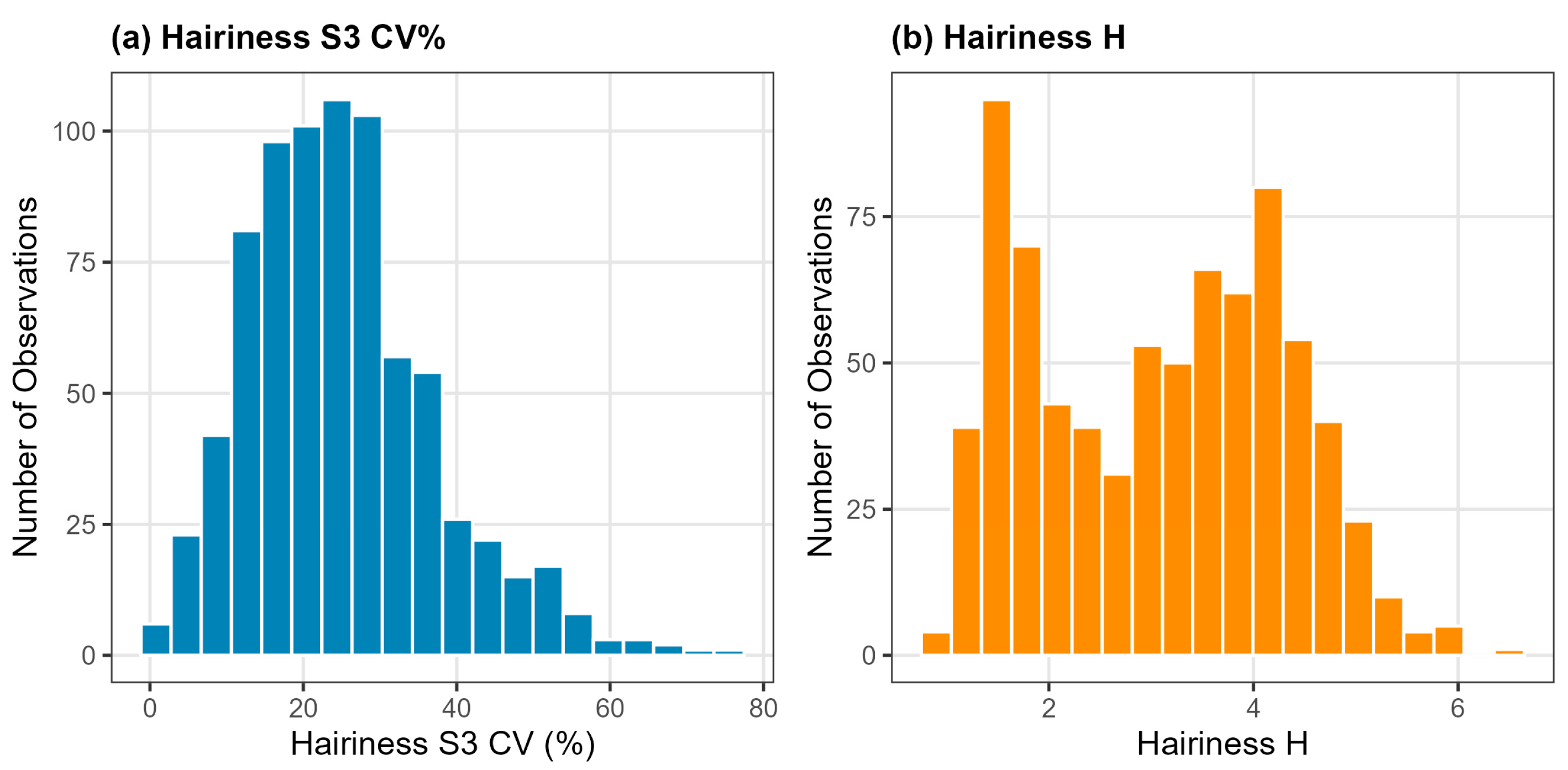
For twist and hairiness H, the null hypothesis that the data follow a single Poisson or gamma distribution is rejected decisively (p < 0.001), providing strong statistical evidence that a single-distribution model is inadequate and that a mixture representation is warranted. For hairiness S3 CV%, by contrast, the single gamma distribution is not rejected at the conventional level (p = 0.053), and we therefore do not treat the chi-square result as establishing its inadequacy for this variable. The descriptive characteristics of the two hairiness indices differ in a manner consistent with their eventual model orders: the histogram of H in Figure 1 shows clearly separated modes, in agreement with its negative excess kurtosis (−1.113), whereas S3 CV% is unimodal with pronounced right skew. We note that right skew alone would not indicate latent structure, since a single gamma or lognormal density can generate strong skew. The evidence for a two-component representation of S3 CV% therefore rests on the AIC/BIC comparison, in which the two-component model improves substantially on the single distribution. This pattern, in which a formal single-distribution test is only marginally rejected while information-criterion comparison provides much stronger discriminating power, has been previously reported in mixture-model applications to skewed engineering data.

The pronounced excess kurtosis of the twist distribution (7.003) is particularly notable and is consistent with the presence of a small, distinct sub-population of high-twist observations superimposed on the bulk of the data.

3.2. Distribution Fitting of the Twist Parameter

A Poisson mixture distribution was first applied to the twist dataset following the unified EM framework of Section 2.3, with K = 1 to 4 components compared via AIC and BIC in

Table 2. Model comparison for the twist parameter (Poisson mixture distribution, n = 769).

K	logLik	AIC	BIC
1	−4037.773	8077.546	8082.191
2	−3510.603	7027.205	7041.141
3	−3510.603	7031.205	7054.431
4	−3510.603	7035.205	7067.721

.

The log-likelihood improves sharply from K = 1 to K = 2, by 527.17 units, but does not improve at all beyond K = 2. BIC, which penalizes the additional parameters of the K = 3 and K = 4 models, therefore identifies K = 2 as optimal. The exact equality of the log-likelihoods across the three higher orders requires explanation, and

Table 3. Poisson mixture components at K = 2, 3 and 4 for twist.

K	Weights	λ	logLik
2	0.922, 0.078	727.315, 871.370	−3510.603
3	0.891, 0.031, 0.078	727.315, 727.315, 871.370	−3510.603
4	0.825, 0.098, 0.004, 0.074	727.315, 727.315, 871.370, 871.370	−3510.603

provides it.

At K = 3 and K = 4 the additional components reproduce the intensity parameters of the two-component solution exactly, redistributing the existing mixing proportions without altering the fitted distribution. The equality of the log-likelihoods therefore reflects exact component redundancy. No component approaches a boundary of the parameter space, and all 1000 random initializations converge to the same optimum, which excludes both boundary solutions and convergence failure as alternative explanations.

Retaining K = 2, the adequacy of the Poisson specification itself was then examined. Assigning each observation to its posterior modal component allows the equidispersion restriction to be assessed directly, and

Table 4. Within-component dispersion of the twist data.

Component	n	Observed Mean	Observed Variance	Variance Implied by Poisson	Dispersion Index D
1690 to 750 t/m	709	727.31	102.76	727.32	0.141
2834 to 874 t/m	60	871.33	101.24	871.37	0.116

reports the resulting within-component moments.

Under a Poisson component the conditional variance equals the conditional mean, so a dispersion index of unity is required. The observed within-component indices are 0.141 and 0.116, corresponding to variances of approximately 14 percent and 12 percent of the values implied by the fitted Poisson means. The twist data are therefore substantially underdispersed relative to the Poisson restriction. This concerns model specification rather than interpretation, and it motivates the comparison of distributional families reported next.

Three specifications were fitted with K = 2. The ordinary Poisson mixture serves as the baseline. A homoscedastic Gaussian mixture was fitted as a continuous alternative, using a common variance across components so that the variance collapse characteristic of unconstrained Gaussian mixtures does not arise. The generalized Poisson mixture of Section 2.3 retains integer support while permitting underdispersion. The results are given in

Table 5. Comparison of distributional specifications for twist, K = 2.

Specification	Parameters	logLik	AIC	BIC	Component Means	Mixture SD	Within-Component D
Poisson mixture	3	−3510.603	7027.21	7041.14	727.32, 871.37	47.22	1 by construction
Homoscedastic Gaussian mixture	4	−3081.525	6171.05	6189.63	727.31, 871.33	39.93	Not applicable
Generalized Poisson mixture	5	−3067.221	6144.44	6167.67	727.31, 871.33	39.84	0.130, 0.106
Observed data						39.96	0.141, 0.116

.

All three specifications recover the same two-component structure, with mixing proportions of approximately 0.922 and 0.078 and component means of approximately 727 and 871 t/m. The principal structural finding is therefore not an artifact of the distributional assumption. The fit statistics, however, differ substantially. The Poisson mixture is inferior to both alternatives, and its implied mixture standard deviation of 47.22 overstates the observed value of 39.96, whereas the generalized Poisson mixture yields 39.84. The fitted dispersion indices of the generalized Poisson components, 0.130 and 0.106, closely reproduce the observed within-component values of 0.141 and 0.116. The generalized Poisson mixture is accordingly adopted as the primary specification for twist, with the Poisson mixture retained as the nested baseline against which it is compared.

Model order was then re-examined under the adopted specification, with results in

Table 6. Model order selection for the generalized Poisson mixture, twist.

K	Parameters	logLik	AIC	BIC
1	2	−4037.773	8079.55	8088.84
2	5	−3067.220	6144.44	6167.67
3	8	−2872.177	5760.35	5797.52

.

Two of the three components lie on the boundary of the admissible region defined in Section 2.3. The first has λ = 0, at which the generalized Poisson distribution reduces to the ordinary Poisson, and the second has λ = −3, the lower bound imposed in estimation. The consequence is visible in the fitted probabilities. The third component carries a weight of 0.263 and is centred at 872.61 t/m, so the model assigns approximately 26 percent of the probability to the region above 840 t/m, whereas only 7.3 percent of the observations lie there. The K = 3 solution therefore attains a higher likelihood while describing the data less accurately than the K = 2 solution. The latter is retained, and its parameter estimates are given in

Table 7. Fitted generalized Poisson mixture parameters for twist, K = 2.

Component	w	θ	λ	Mean	Variance	SD	D
1	0.92198	2014.340	−1.76959	727.31	94.82	9.74	0.130
2	0.07802	2682.580	−2.07871	871.33	91.93	9.59	0.106

.

The fitted mixture identifies a dominant component with weight 0.922 centered at 727.31 t/m, alongside a smaller component with weight 0.078 centered at a substantially higher level, 871.33 t/m. The separation between the two component means is approximately 144 t/m, roughly 3.6 standard deviations of the overall data, and is large relative to the pooled variability. This explains both the marked excess kurtosis reported in Table 1 and the strong rejection of the single-distribution hypothesis. Physically, this two-population structure is consistent with occasional over-twisting episodes arising from ring-frame spindle-speed variation, from incorrect twist-multiplier settings during a subset of production lots, or from drafting-system irregularities superimposed on an otherwise tightly controlled target twist level. This pattern is broadly consistent with the twist-strength trade-off described by Palaniswamy and Mohamed [16] and Patil et al. [17], who note that twist stability is highly sensitive to ring-frame process settings.

Substituting the parameters of Table 7 into the generalized Poisson mixture density gives

$$\begin{array}{c}f{\left(x\right)}_{\mathrm{twist}}=0.92198\left[{\displaystyle \frac{2014.340{\left(2014.340-1.76959x\right)}^{x-1}{e}^{-2014.340+1.76959x}}{x!}}\right]+\\ 0.07802\left[{\displaystyle \frac{2682.580{\left(2682.580-2.07871x\right)}^{x-1}{e}^{-2682.580+2.07871x}}{x!}}\right]\end{array}$$

(22)

Figure 2 overlays the observed histogram with a sample simulated from this fitted mixture. The two distributions agree in the location and relative weight of the components and in overall spread, the simulated standard deviation being 39.84 against an observed value of 39.96. A formal assessment of distributional adequacy is reported in Section 3.4.

The first two moments of the fitted mixture are compared with their empirical counterparts in

Table 8. Mean and standard deviation of twist: observed data versus generalized Poisson mixture model.

Data	Obs. Mean	Obs. SD	GPMM Mean	GPMM SD
Twist (t/m)	738.54	39.96	738.54	39.84

.

The theoretical mixture mean matches the observed mean to three decimal places, and the theoretical standard deviation of 39.84 closely matches the observed value of 39.96. The corresponding Poisson mixture implies a standard deviation of 47.22, which overstates the observed dispersion. Relaxing the equidispersion restriction therefore improves agreement with the second moment of the data as well as with the information criteria.

Twist is supported on six recorded levels, with 85.3 percent of observations at a single value, so any continuous or semi-continuous fitted function is necessarily flatter at those levels than the empirical frequencies. The adequacy of the fitted mixture is therefore assessed numerically, through the moment comparison in Table 8 and the goodness-of-fit results reported in Section 3.4.

3.3. Distribution Fitting of the Hairiness (S3 CV%, H)

The two hairiness indices were each modeled independently using the gamma mixture distribution framework, since, although both quantify aspects of the same physical phenomenon [11], they capture materially different features of the hairiness distribution: S3 CV% reflects the coefficient of variation of long-hair counts, while H reflects the equivalent hairy surface area, and their marginal distributions accordingly differ substantially in shape. Model comparison results are given in

Table 9. Model comparison for hairiness S3 CV% and H (gamma mixture, n = 769).

Data	K	logLik	AIC	BIC
Hairiness S3 CV%	1	−2989.91	5983.82	5993.11
Hairiness S3 CV%	2	−2973.16	5956.32	5979.55
Hairiness S3 CV%	3	−2972.87	5961.73	5998.89
Hairiness S3 CV%	4	−2970.56	5963.12	6014.22
Hairiness H	1	−1237.43	2478.87	2488.16
Hairiness H	2	−1113.35	2236.70	2259.93
Hairiness H	3	−1098.58	2213.16	2250.32
Hairiness H	4	−1095.41	2212.81	2263.91

.

For hairiness S3 CV%, both AIC and BIC are minimized at K = 2. For hairiness H, BIC is minimized at K = 3; although AIC is marginally lower at K = 4, the difference is negligible and BIC clearly favors the more parsimonious K = 3 solution. Accordingly, a two-component mixture model is used for hairiness S3 CV% and three-component mixture for hairiness H in the analyses that follow. The fitted parameters are summarized in

Table 10. Gamma mixture distribution parameters for hairiness S3 CV% and H.

Data	K	π1	π2	π3	(α1,β1)	(α2,β2)	(α3,β3)
Hairiness S3 CV%	2	0.036	0.964	-	(2.96, 0.63)	(4.82, 0.19)	-
Hairiness H	3	0.091	0.315	0.594	(200.94, 142.69)	(16.32, 8.43)	(32.49, 8.25)

.

For S3 CV%, the mixture reveals a highly asymmetric structure: a small component (π₁ = 0.036, mean = α₁/β₁ ≈ 4.69) represents a small minority of records with atypically low reported hair-count variability, while the large majority of samples (π₂ = 0.964, mean ≈ 25.76) exhibit the typical, considerably more variable hairiness behavior of routine production. The shape parameters of both components indicate that each subpopulation is itself right-skewed, so that the overall skewness of the S3 CV% distribution arises from a combination of within-component skew and between-component separation. This finding is consistent with the general observation in the hairiness literature that S3-type indices are highly sensitive to occasional fibre-feeding or drafting disturbances that produce a small subset of outlying, highly variable bobbins.

For H, the mixture instead reveals a three-component structure: a small and exceptionally homogeneous low-H subpopulation, a more dispersed low-to-moderate component, and a dominant, moderately dispersed high-H component. This suggests that, unlike S3 CV%, the H index distinguishes three distinct production regimes rather than two, potentially corresponding to different spindle groups, shifts, or raw material batches, a distinction that would not be visible under a single-component assumption.

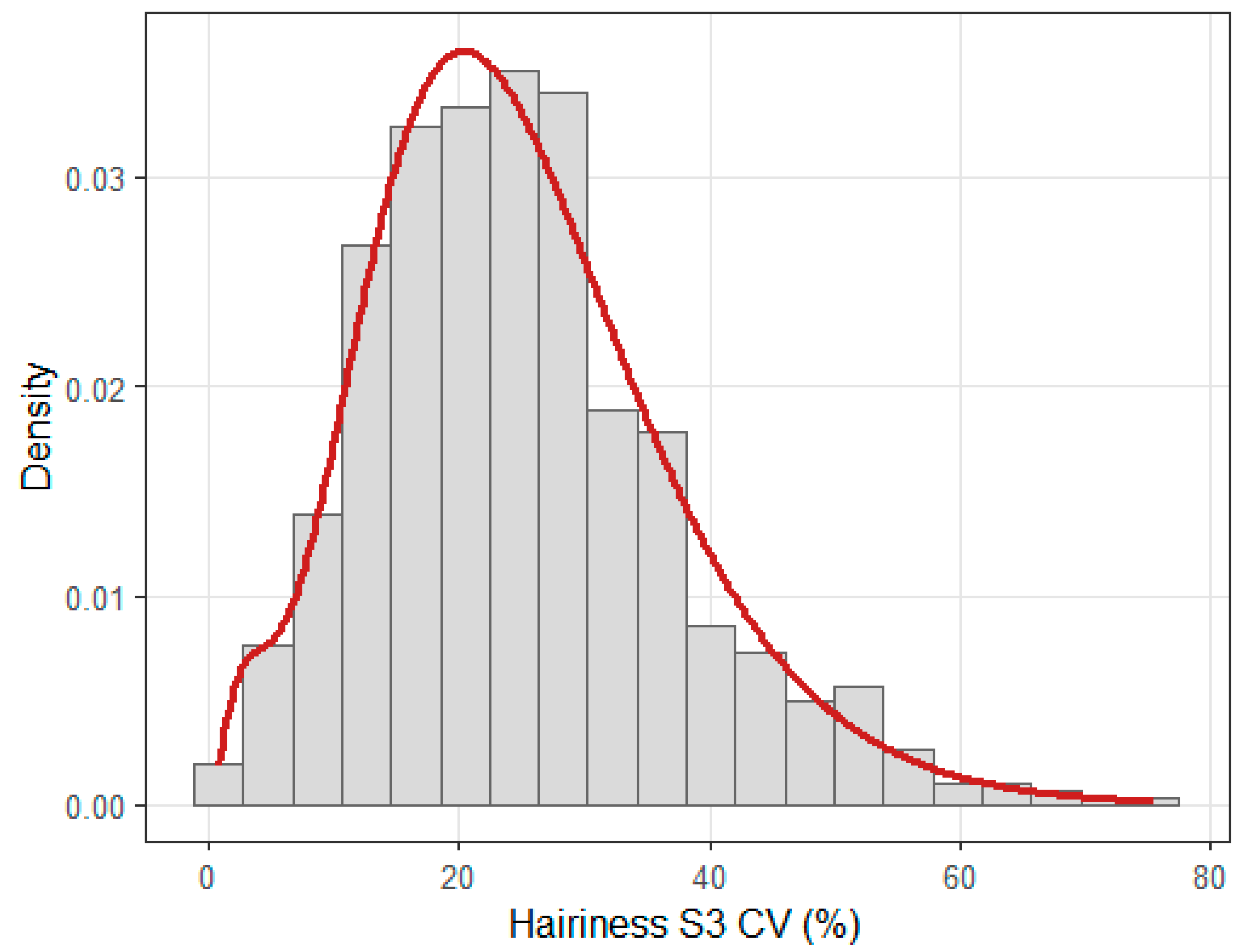
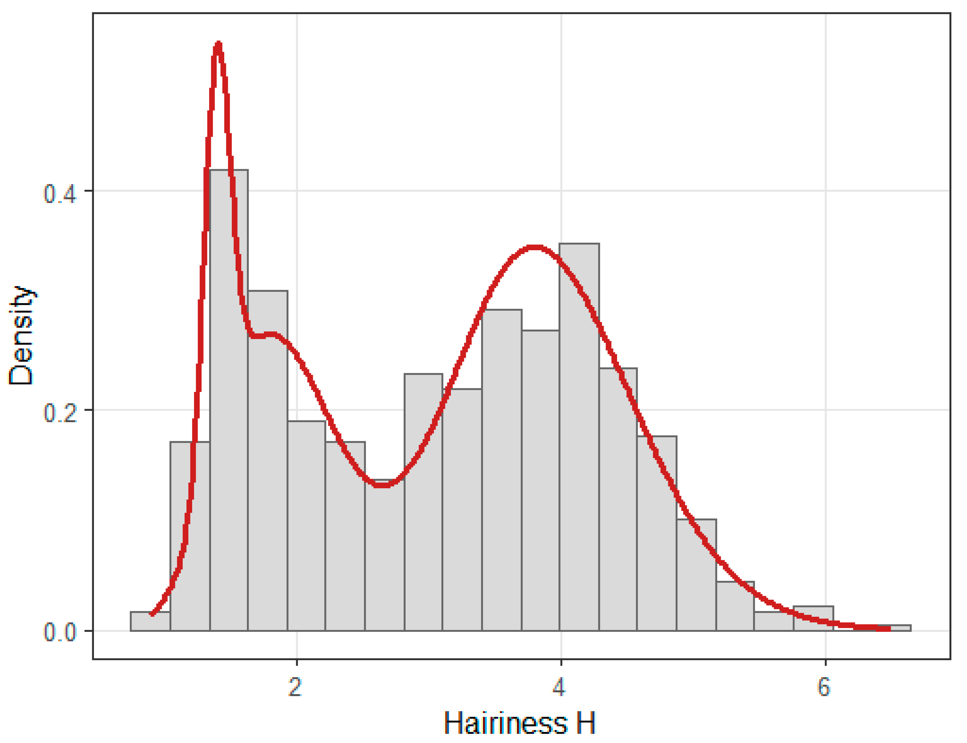
The visual adequacy of the fitted gamma mixtures is illustrated in Figure 2 and Figure 3. Figure 2 overlays the observed S3 CV% histogram with a histogram simulated from the fitted two-component mixture; the pronounced right-skewed shoulder and the long right tail of the observed data are both closely reproduced by the simulated distribution, visually corroborating the two-component structure identified in Table 6.

Figure 3 presents the analogous comparison for H, where the simulated histogram closely tracks the multi-modal shape of the observed data, consistent with the three components (π₁ = 0.09 at mean ≈ 1.41, π₂ = 0.32 at mean ≈ 1.94, π₃ = 0.59 at mean ≈ 3.94) reported above.

Table 11. Mean, standard deviation, and goodness-of-fit results: observed data vs. fitted gamma mixture model.

Data	K	Obs. Mean	Obs. SD	Model Mean	Model SD	MWU p	K-S p	AD p
Hairiness S3 CV%	2	25.00	12.22	25.00	12.18	0.21	0.83	0.96
Hairiness H	3	3.08	1.21	3.08	1.21	0.68	0.42	0.62

summarizes the agreement between the observed data and each fitted gamma mixture model across three complementary diagnostics. The Mann–Whitney U results are reported for completeness but, as noted in Section 2.6, they concern stochastic ordering rather than distributional equality.

For both indices, the model-implied mean matches the observed mean, and standard deviation is within 0.3% (S3 CV%) and 0% (H) of the observed value, indicating that the fitted mixtures reproduce not only central tendency but also the overall dispersion of each parameter. The Kolmogorov–Smirnov and Anderson–Darling tests yield p-values well above the conventional 0.05 threshold for both indices.

Substituting the parameters of Table 10 into Equation (14) gives the fitted density functions:

$$f{\left(x\right)}_{S3\hspace{0.17em}\mathit{CV}\%}=0.036\cdot \left[{\displaystyle \frac{{0.63}^{2.96}\hspace{0.17em}{x}^{1.96}\hspace{0.17em}{e}^{-0.63x}}{\mathsf{\Gamma }\left(2.96\right)}}\right]+0.964\cdot \left[{\displaystyle \frac{{0.19}^{4.82}\hspace{0.17em}{x}^{3.82}\hspace{0.17em}{e}^{-0.19x}}{\mathsf{\Gamma }\left(4.82\right)}}\right]$$

(23)

$$\begin{array}{c}f{\left(x\right)}_H=0.091\cdot \left[{\displaystyle \frac{{142.69}^{200.94}{x}^{199.94}{e}^{-142.69x}}{\mathsf{\Gamma }\left(200.94\right)}}\right]+0.315\cdot \left[{\displaystyle \frac{{8.43}^{16.32}{x}^{15.32}{e}^{-8.43x}}{\mathsf{\Gamma }\left(16.32\right)}}\right]+\\ 0.594\cdot \left[{\displaystyle \frac{{8.25}^{32.49}{x}^{31.49}{e}^{-8.25x}}{\mathsf{\Gamma }\left(32.49\right)}}\right]\end{array}$$

(24)

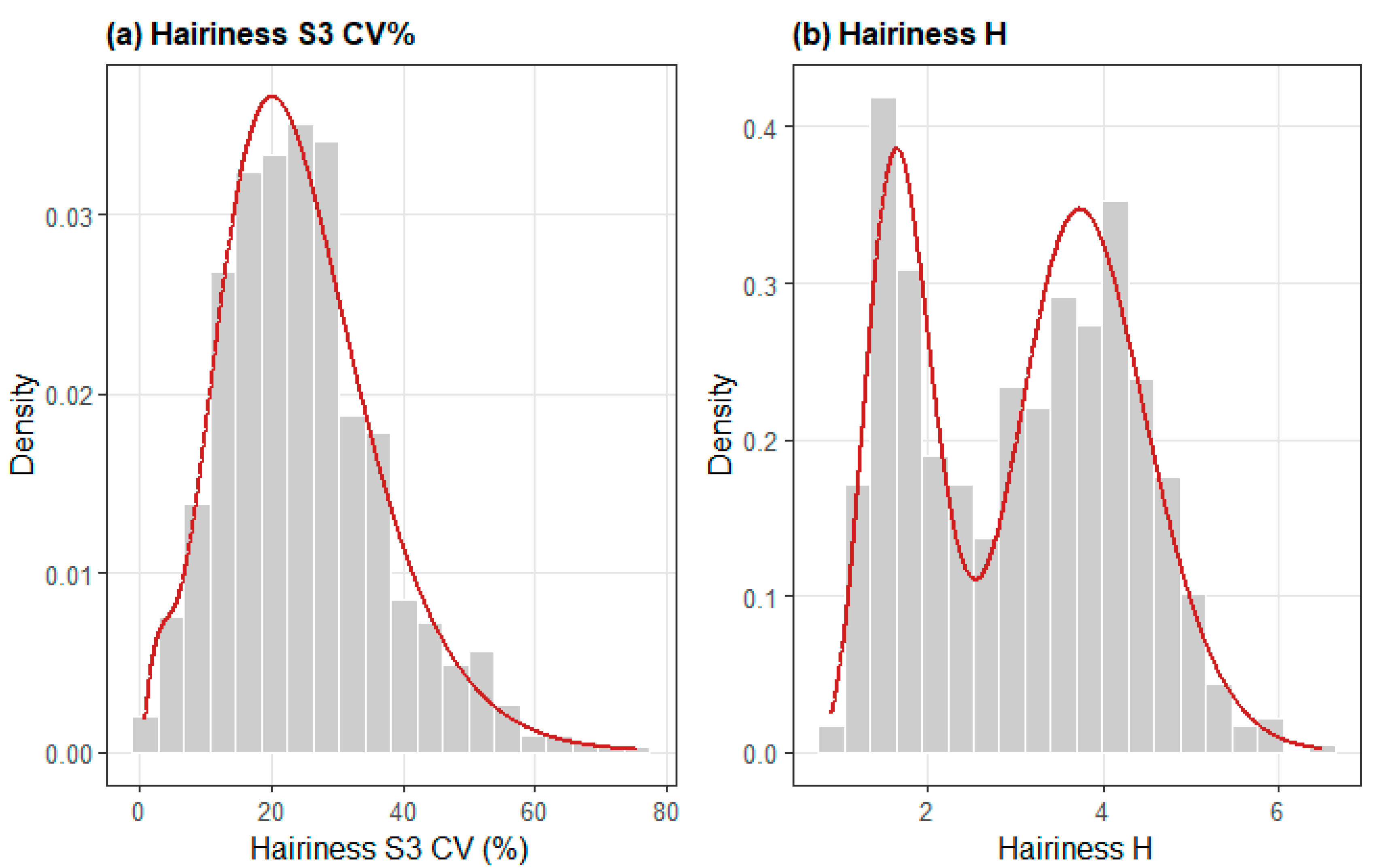
Figure 4 overlays these fitted densities on the observed histograms. For S3 CV% in Figure 4a, the curve tracks both the bulk of the distribution and its upper tail, the latter arising from the right skew of the dominant component rather than from the small low-mean component. For H in Figure 4b, the fitted density reproduces both principal modes and the intervening trough, confirming that the three-component mixture captures the multi-modal shape of the variable and the narrow spread of its low-H component.

Three findings stand out from this synthesis. First, model order is not uniform across parameters. A two-component mixture is optimal for hairiness S3 CV%, extending the two-latent-subpopulation structure previously reported for yarn imperfection parameters in our companion study, while hairiness H requires a three-component mixture, indicating a more granular latent segmentation. Second, the degree of separation between components differs markedly by parameters. Hairiness S3 CV% shows a small, well-separated minority component consistent with occasional process excursion, whereas hairiness H shows a more graded three-way split consistent with multiple, more comparably sized production regimes. This distinction has direct practical implications for quality control: parameters with a rare, well-separated component are better targeted by outlier-detection strategies focused on identifying the specific lots or spindles responsible for the minority component, whereas parameters with a graded multi-component structure may instead call process-level investigation of the systematic factors distinguishing the regimes. Third, the mixture-implied mean and standard deviation matched their observed counterparts closely for both indices. The formal assessment of distributional adequacy is reported in Section 3.4, where the gamma mixture for S3 CV% is not rejected while residual departures remain for H.

3.4. Initialization Sensitivity and Goodness of Fit

Table 12. Initialization sensitivity of the fitted mixtures.

Model	Random Starts	Structured Starts	Retained logLik	Random Starts Attaining It	Range of Attained logLik
Twist, K = 2	1000	5	−3510.603	100%	−3510.603 to −3510.603
S3 CV%, K = 2 gamma	500	5	−2973.162	0%	−2973.855 to −2973.852
H, K = 3 gamma	500	5	−1098.580	99%	−1101.099 to −1098.580

reports the outcome of the initialization procedure described in Section 2.5.

All five structured initializations converged to the retained optimum for each model. For twist the likelihood surface is unimodal in practice, since every random start reached the same solution. For S3 CV% no random start recovered the retained optimum, all terminating at a nearby inferior stationary point near −2973.85. The cause is that assigning random posterior weights to all 769 observations makes the two components nearly identical at the first M-step, which is the situation that arises when one mixing proportion is small. The solutions reported above are those attained by the structured initializations and, where applicable, confirmed by the random starts.

Distributional adequacy was assessed by parametric bootstrap in

Table 13. Parametric bootstrap goodness-of-fit results.

Model	KS	p	CvM	p
S3 CV%, single gamma	0.0323	0.037	0.146	0.043
S3 CV%, K = 2 gamma	0.0241	0.152	0.0488	0.238
H, K = 2 gamma	0.0406	0.007	0.1374	0.013
H, K = 3 gamma	0.0292	0.013	0.0780	0.007
Twist, Poisson mixture	0.4403	0.003	40.399	0.003
Twist, generalized Poisson mixture	0.5115	0.003	44.678	0.003

. For each fitted model, replicate samples of size n = 769 were generated from the fitted distribution, the model was re-estimated on every replicate, and the Kolmogorov–Smirnov and Cramer–von Mises statistics were recomputed to obtain a reference distribution. This procedure accounts for the fact that the parameters under test are estimated from the same data.

For S3 CV% the procedure supports the modeling strategy on a proper inferential basis. The single gamma distribution is rejected by both statistics, while the two-component mixture is not rejected. For H, the three-component model reduces the Kolmogorov–Smirnov statistic from 0.0406 to 0.0292 and improves BIC, so it captures the dominant multi-modal structure, but systematic residual departures remain and neither the two- nor the three-component mixture for H is accepted at conventional levels.

For twist, both the Poisson and the generalized Poisson mixtures are rejected. This outcome has a structural cause. The twist variable is supported on six distinct recorded values, with 85.3 percent of observations at a single value, and no continuous or semi-continuous distributional family can reproduce a distribution of this shape. The generalized Poisson mixture attains larger values of both statistics than the Poisson mixture, for the reason given in the following paragraph, but improves substantially on it in every other respect, reducing BIC by 873 units and reproducing both the observed within-component dispersion and the observed mixture standard deviation. It is retained as the best available representation among the specifications considered, and because the two-component structure it identifies is common to all three families examined, rather than as a distributionally adequate description of the twist data. The implications for interpretation are stated in Section 4.

The statistics for twist are an order of magnitude larger than those for the hairiness indices, and they are slightly larger for the generalized Poisson mixture than for the Poisson mixture. Both features follow from the discrete support of the variable. The empirical distribution function rises from 0.066 to 0.919 at the single value 730 t/m, so the supremum difference is governed by the probability each model assigns below that point. The generalized Poisson components are narrower than the Poisson components and place 0.578 of the probability mass below 730 t/m against 0.507 for the Poisson specification, which increases the discrepancy at the lower edge of the step even though the fit improves on every other criterion. Empirical distribution function statistics therefore do not discriminate usefully between specifications for a variable of this kind, and the preference for the generalized Poisson mixture rests on the likelihood, the information criteria and the agreement of the first two moments.

4. Conclusions

This study extended the finite mixture modeling (FMM) framework previously validated for yarn imperfections and mechanical properties [10] to a new set of yarn quality parameters in a 28/1 Ne ring-spun polyester/viscose yarn. Using a generalized Poisson mixture for the integer-valued twist parameter and gamma mixtures for the continuous hairiness parameters, and selecting model order through a systematic AIC and BIC procedure, the results demonstrated that a two-component mixture provides the optimal representation for twist and for hairiness S3 CV%, while hairiness H required a three-component mixture. In each case the selected mixture decisively outperformed the corresponding single-distribution model in terms of information criteria. Each fitted model was further assessed by the close numerical agreement between the theoretical mixture mean and standard deviation and their empirical counterparts, and by parametric bootstrap goodness-of-fit testing. The two-component gamma mixture for S3 CV% was not rejected by that procedure, whereas residual departures remained for H and for twist.

These findings extend, and are consistent with, the growing body of evidence that industrial and engineering process data are frequently better described by a small number of latent subpopulations than by a single parametric distribution [1,2,21]. The consistent selection of mixture distribution models across all three parameters mirrors the two-component structure previously reported for thin places, thick places, neps, tenacity, and elongation in ring-spun polyester/viscose yarn [10], as well as the two-component Weibull mixtures long established for cotton fiber length distributions [5,6,7,8,9]. Taken together with these precedents, the present results suggest that a two-component mixture may represent a recurring, and perhaps generic, signature of ring-spinning process data, plausibly reflecting the coexistence of an “in-control” production regime with a secondary regime associated with specific machine settings, raw-material batches, or occasional process excursions—an interpretation broadly consistent with mixture-model applications to process-monitoring and reliability data in other manufacturing contexts [3,4].

At the same time, the study revealed that the nature of the two-component structure differs meaningfully across parameters, with direct implications for how the underlying quality-control literature should be interpreted and applied. For twist, the fitted mixture separated a small (7.8%), markedly higher-twist subpopulation (λ₁ = 871.37 t/m) from the dominant production regime (λ₂ = 727.32 t/m, 92.2%); this rare-excursion pattern is consistent with the established sensitivity of twist to ring-frame spindle-speed and twist-multiplier settings emphasized by Palaniswamy and Mohamed [16] and by Patil et al. [17], who note that even modest deviations from target twist settings can propagate into detectable shifts in yarn structure and strength. The present results extend this qualitative understanding by providing, for the first time to our knowledge, an explicit probabilistic characterization of how much of the production is affected by such excursions and by how much the affected subpopulation deviates from target.

From an applied perspective, these findings reinforce the practical value of the FMM approach for yarn quality control demonstrated in our companion study. Because each fitted mixture yields an explicit, closed-form probability density function, quality engineers can directly compute the probability that a given parameter falls outside a specification limit, monitor drift in individual component means or weights over time as an early-warning indicator of process excursions.

This study has several limitations that suggest directions for future research. First, the analysis was based on a single yarn construction (28/1 Ne ring-spun, combed PE/V 65/35) and a specific subset of the manufacturer’s test records (n = 769) obtained from a single manufacturing facility. Therefore, although mixture representations consistently outperformed single distributions for the parameters examined in this study, this structure should not be interpreted as a universal characteristic of ring-spun yarn production. The identified mixture structure may partly reflect the specific raw materials, machine settings, and operating conditions of the investigated production environment. Future studies should validate the proposed FMM framework across different yarn counts, fiber blends, spinning conditions, and manufacturing facilities to determine whether the observed component structures represent recurring patterns across broader production contexts or is specific to particular yarn and process configurations.

A methodological limitation concerns the distributional formulation adopted for the twist data. The ordinary Poisson mixture, which matches the integer-valued turn-count measurements, imposes equality of the conditional mean and variance, and the observed within-component dispersion indices of 0.141 and 0.116 depart substantially from the required value of unity. The generalized Poisson mixture adopted here relaxes this restriction while preserving integer support, and it reproduces the observed within-component dispersion and the observed mixture standard deviation closely. It nevertheless does not provide an adequate description of the full twist distribution, as reported in Section 3.4. The two-component structure identified for twist is common to the Poisson, homoscedastic Gaussian and generalized Poisson specifications, so it does not depend on the distributional assumption, but the twist results should be read as identifying the number and location of latent groups rather than as a distributional model of the variable.

Another limitation concerns the interpretation of the identified latent components. Although the fitted mixture models provide a statistical characterization of heterogeneity in the observed data, the historical dataset does not contain observation-level information on raw-material lots, production shifts, individual machines, maintenance or calibration conditions, or process settings that would allow the operational origins of the identified components to be determined. Consequently, although the latent components may potentially be associated with differences in machine conditions, process settings, raw-material batches, or other production-related factors, such relationships cannot be established from the available data. Future studies should integrate posterior component-membership probabilities with observation-level production and process variables to investigate whether particular latent subpopulations are systematically associated with specific operating conditions. Such analyses could help establish links between statistically identified heterogeneity and its potential production-related sources, thereby supporting more targeted process monitoring and quality-control strategies.

The twist analysis identifies a two-component structure that is reproduced by three distinct distributional families, but no member of those families provides an adequate description of the full twist distribution. The variable takes only six distinct recorded values, and the discreteness of its support is more pronounced than any of the specifications considered can accommodate. Results concerning twist should therefore be read as identifying the number and location of latent groups rather than as a distributional model of the variable. Approaches designed for data on a small discrete support, such as latent class models with categorical outcomes or models treating the recorded levels as ordered categories, would be the appropriate next step.

The 769 records were collected sequentially over an extended production period, which raises the possibility of clustering by machine, batch or sampling occasion, or of serial dependence between temporally adjacent tests. Observation-level identifiers for machine, raw material lot and shift were not retained in the quality control database, so clustering cannot be tested directly. As a partial check, serial correlations of the observation sequence were computed. For S3 CV% these are 0.015 at lag one and 0.029 at lag two, and for H they are 0.055 and 0.030, all negligible relative to the threshold of approximately 0.071 implied by the sample size. This supports treating the records as approximately independent for estimation purposes, but it does not exclude clustering at levels the recorded ordering does not reveal. Should such clustering be present, the effective sample size would be smaller than 769, standard errors and information criteria would be optimistic, and the estimated components might partly reflect grouping structure rather than intrinsic yarn populations. A hierarchical or mixed effects mixture formulation applied to data carrying batch and machine identifiers would be the appropriate way to address this.

In summary, this study demonstrates that finite mixture models provide a statistically rigorous and practically informative framework for characterizing the heterogeneity of key yarn structural and mechanical parameters, extending the applicability of this modeling approach beyond the yarn imperfection parameters previously studied to a broader set of quality characteristics relevant to weaving, knitting, and fabric-appearance performance. The consistent multi-component structure identified across the three parameters examined, together with the qualitatively distinct interpretations supported by the existing textile literature [15,16,17,34], underscores both the generality of the FMM approach and the importance of parameter-specific interpretation when translating statistical findings into quality-control practice.