Thermomechanical Stress Response of Mechanically Lined Pipes Under Combined Loading

Abstract

Mechanically lined pipes (MLP) combine a carbon-steel base pipe with a thin corrosion-resistant liner that transfers load through frictional contact. This numerical study compares the stress responses of matched monometallic and mechanically lined pipes under prescribed internal pressure, temperature, and bending. Three-dimensional finite element models are used to represent the material layers, contact, friction, and thermal loading. Circumferential mesh refinement and comparison with field inspection data provide checks on the reported stress response. In the non-bending one-factor cases, pressure and diameter primarily affect equivalent stress, whereas increasing temperature increases liner compression and base-pipe equivalent stress. At constant total wall thickness, increasing liner thickness reduces liner compression but increases stress in the thinner base pipe. Bending increases both response measures. Local sensitivity and two-factor analyses characterize stress variations within the sampled conditions. Exploratory regression equations show high internal cross-validation accuracy, and on 22 finite-element cases, the unchanged regression equations achieved R² values of 0.965 for liner stress and 0.986 for base-pipe stress. These results support stress-trend estimation within the tested conditions but do not establish accuracy for arbitrary five-factor combinations or a universal failure threshold.

1. Introduction

Mechanically lined pipes (MLP) combine a carbon-steel base pipe, which carries the principal structural loads, with a thin corrosion-resistant liner. In steep mountainous terrain, pressure and thermal expansion may act together with quasi-static bending caused by slope movement, differential settlement, or local free spanning. The response depends on the stress state in each layer and load transfer across the interface. A homogeneous-pipe model cannot directly resolve this interlayer stress partitioning.

Early research on bimetallic pipes focused on manufacturing, interfacial bonding, and material compatibility. Yan et al. [1] reviewed composite-pipe products and development trends. Wu et al. [2] developed a parametric model for three-roll skew rolling, while Dong et al. [3] combined forming simulations with experiments. Ji and Huang [4] classified solid–solid, solid–liquid, and liquid–liquid composite mechanisms, emphasizing the influence of the manufacturing route on the initial interface. Later structural studies showed that residual stress, geometry, loading path, pressure, and friction affect liner instability [5]. These findings motivate explicit representation of the interface when examining layered-pipe stress responses.

Liner behavior under bending, reeling, and pressure has received sustained attention. Nonlinear analyses have examined detachment, wrinkling, and secondary bifurcation [6], while other studies considered initial prestress, repeated loading, plastic bifurcation, collapse near girth welds, and cyclic reel-lay response [7,8,9,10,11]. Low to moderate internal pressure can restrain ovalization and delay wrinkling [12,13]. Hydraulic expansion establishes residual contact pressure that helps maintain composite action [14], and friction affects the response under bending [15]. Related studies have examined external-pressure collapse prediction and lateral crushing [16,17]. These studies provide context for the present stress analysis; minimum principal stress is treated here as a measure of compression rather than a standalone failure criterion.

Geological deformation provides the global action that activates these local mechanisms. Pipeline models have coupled fault or landslide displacement with axial response and beam bending [18]. Other studies quantified soil resistance, diameter-to-thickness ratio, and pressure [19], or included service pressure and temperature in elastoplastic analysis [20]. Fault-crossing angle [21] and moment–curvature response [22] have also been examined. These models explain how ground movement reaches a homogeneous pipeline, but they do not resolve load redistribution across a frictional base-pipe–liner interface.

Finite element parameter studies are often paired with reduced-order regressions to organize large response datasets. Apparent predictive accuracy can be optimistic, however, when the development data comprise one- and two-factor slices rather than a space-filling multivariable design. This statistical limitation is especially important for liner instability because stress does not directly measure strain localization, ovalization, interface opening, or wrinkle growth. The reduced-order equations are therefore used only to describe the sampled response space, not to predict failure or safety.

Recent geometrically nonlinear shell theory can represent large displacement, rotation, and cross-sectional deformation in thin-walled tubes [23]. Such analytical formulations provide an important methodological counterpart for tubular mechanics. The present problem additionally includes nonbonded layers, unilateral contact, Coulomb friction, prescribed thermal loading, and possible local separation. These features motivate a three-dimensional finite element treatment here, but do not make numerical simulation the only possible analytical framework.

The specific contribution is a matched monometallic/MLP comparison that resolves layer-specific stresses under prescribed pressure, temperature, and bending. The study examines how loading and geometry affect base-pipe equivalent stress and liner compression, and how these responses vary when two parameters change together. The scope is limited to structural stress response within the modeled parameter domain.

Three-dimensional finite element models of matched monometallic and mechanically lined pipes are used to compare the effects of pressure, temperature, liner thickness, diameter, and bending moment. Local sensitivities and two-factor response surfaces are then used to examine the parameter-dependent stress variations. Empirical response equations are evaluated by internal cross-validation and 22 independent finite-element cases, and are retained only as exploratory descriptions of the sampled responses.

The applied end moment represents the bending action transmitted by geological deformation; the model does not simulate pipe–soil interaction or landslide evolution. The findings therefore describe structural trends within the modeled parameter domain. Published tests provide qualitative context, but route-specific geohazard analysis, geometry-specific nonlinear verification, and physical testing remain necessary for engineering application.

2. Finite Element Model and Computational Method

2.1. Finite Element Formulation and One-Way Thermal-Structural Implementation

A quasi-static one-way thermal-structural analysis is used. A steady-state thermal analysis was first performed to obtain the temperature field. The transported-fluid temperature was set to 150 °C. Convection was applied to the outer surface of the L360 base pipe with a heat-transfer coefficient of 6 × 10⁻⁶ W mm⁻² °C⁻¹ and to the cylindrical inner surface of the MP35N liner with a heat-transfer coefficient of 8 × 10⁻⁸ W mm⁻² °C⁻¹. The resulting temperature field was transferred to the subsequent structural analysis as a thermal load. No feedback from mechanical deformation to the temperature field was included; therefore, the analysis is not described as fully coupled thermomechanics.

$$\nabla ·\sigma +b=0$$

(1)

where σ is the Cauchy stress tensor (N m⁻²), b is the body force per unit volume (N m⁻³), and ∇ is the spatial gradient operator (m⁻¹). The displacement field is u(x), and it enters the strain through the displacement gradient; in the finite element solution, u is the nodal displacement unknown. Consequently, ∇ × σ has units of N m⁻³, which are consistent with b.

$$\epsilon ={\epsilon }^e+{\epsilon }^p+{\epsilon }^{\mathit{th}}, {\epsilon }^{\mathit{th}}=\alpha (T-T_0)I$$

(2)

The additive elastic, plastic, and thermal-strain notation describes the material inputs and thermal-strain contribution. Both the Large Deflection and Weak Springs options were disabled in ANSYS 2024 R1 Mechanical.

Based on the above strain decomposition, the material stress is determined using the thermo-elastoplastic constitutive relationship:

$$\sigma =C:(\epsilon -{\epsilon }^{\mathit{p}}-{\epsilon }^{\mathit{th}})$$

(3)

Here C is the fourth-order elastic stiffness tensor and “:” denotes the tensor double-dot product. The displayed constitutive notation identifies the elastic and thermal material inputs. The onset of plasticity is evaluated using the von Mises equivalent-stress criterion and the material stress–strain relationship supplied to the solver. The liner minimum principal stress is used only as a local prebuckling compression indicator, not as a validated wrinkling-initiation criterion.

Internal pressure acts as a normal traction on the cylindrical liner inner surface. Pressure-induced end-cap thrust is not applied; the modeled segment therefore represents an open-ended pressure condition. The end moment is introduced as an equivalent cross-sectional load. Temperature is prescribed as a structural thermal load. Two kinematic boundary-condition configurations were used according to the loading objective. For the non-bending one-factor series (internal pressure, temperature, liner thickness, and pipe diameter), the two direct displacement objects were active on the selected end faces at both pipe ends. Their settings were: at one end, UX was free, UY = 0, and UZ = 0; at the opposite end, UX was free, UY = 0, and UZ was free. Because the model uses three-dimensional solid elements, no independent rotational degrees of freedom were prescribed on the directly constrained end faces; only the listed translational components were imposed. Thus, axial movement was restrained at one end and released at the opposite end, allowing axial thermal expansion toward the free end in the non-bending one-factor series. For the one-factor bending series and for all simulations used in the sensitivity and two-factor response-surface analyses, the two direct end-face displacement conditions were suppressed. Instead, flexible MPC coupling was defined between the respective end sections (four selected faces at each end) and two remote reference points. Remote Point, located at Z = −5000 mm, carried a remote displacement with UX = UY = UZ = 0 and RX = RY = RZ = 0. Remote Point 2, located at Z = 0 mm, received the bending moment about the global X-axis; the moment was transmitted to the associated end cross-section through flexible MPC coupling, and its magnitude was varied according to the load case. Thus, in the remote-point configuration, the remote displacement at Remote Point was the only kinematic restraint; Remote Point 2 served as the moment-application point and had no prescribed displacement or rotation. Suppressing the direct end-face displacement conditions avoided redundant kinematic constraints while applying the bending load. In the remote-point configuration used for the bending, sensitivity, and two-factor response-surface analyses, Remote Point 2 had no prescribed axial displacement (UZ) or rotation, so axial thermal expansion could be released toward that end. In the 13 MPa reference condition, internal pressure was applied as a normal traction to the cylindrical inner surface of the MP35N liner; the pressure value was varied in the pressure-dependent series.

$$g_n\ge 0, p_n\ge 0, g_n{p}_n=0, \parallel {\tau }_t\parallel \le \mu p_n\sqrt{b^2-4\mathit{ac}}$$

(4)

where g_n is the normal gap, p_n is the normal contact pressure, τ_t is the tangential contact stress, and μ is the friction coefficient. The first three relations constitute the normal complementarity conditions, while the final relation represents the Coulomb friction constraint. These conditions enable the two material layers to transfer normal pressure and tangential traction while permitting relative sliding when the contact conditions are satisfied.

The weak form of the governing equations is spatially discretized using the finite element method, and the discretized equilibrium equation is solved iteratively within each load increment:

$$K\Delta u=R_{\mathit{ext}}-R_{\mathrm{int}}$$

(5)

The weak form is spatially discretized and solved incrementally. The tangent stiffness is updated as the configuration, contact state, and material response evolve. The model is implemented in ANSYS Workbench using Engineering Data, Geometry, Mechanical, and the Static Structural solver. This implementation description identifies the analysis scope; it is not a substitute for an archived solver-input package containing all coupling and constraint details.

2.2. Geometric Models and Material Parameters

To ensure a consistent comparison, the monometallic and mechanically lined pipes have identical outer diameters, total wall thicknesses, and effective lengths. Their configurations and elastic-thermal material parameters are summarized in

Table 1. Material parameters used in the matched pipe models.

Component	Material	Elastic Modulus	Poisson Ratio	Thermal Expansion
Base pipe	L360	200 GPa	0.30	11.9 × 10−6 K−1
Liner	MP35N	210 GPa	0.31	14.4 × 10−6 K−1
Monometallic pipe	L360	200 GPa	0.30	11.9 × 10−6 K−1

. The mechanically lined pipe consists of an L360 base pipe and an MP35N liner; MP35N is a high-strength nickel–cobalt–chromium–molybdenum corrosion-resistant alloy. Both L360 and MP35N were modeled using bilinear isotropic hardening. For L360, the elastic modulus, Poisson’s ratio, yield strength, and tangent modulus were 200 GPa, 0.30, 360 MPa, and 2.0 GPa, respectively. For MP35N, the corresponding values were 210 GPa, 0.31, 400 MPa, and 2.5 GPa, respectively.

Because the two layers are modeled as nonbonded contacting surfaces with frictional sliding, the configuration considered here is specifically a mechanically lined pipe rather than a metallurgically bonded clad pipe.

The matched models isolate material layering and interfacial constraint. The MLP has a 12 mm L360 base pipe and a 3 mm MP35N liner; the monometallic reference has a 15 mm L360 wall. Both models have a 323.9 mm outer diameter and a 5000 mm length. The baseline MLP starts from nominally contacting, stress-free layers with no deliberately imposed gap, interference, manufacturing-induced residual contact pressure, or residual stress. This idealization is not mechanically equivalent to a manufactured hydraulically or mechanically expanded MLP. The friction coefficient is fixed at μ = 0.20 in the present model and is not varied in the present study. These initial-interface assumptions limit transfer of the results to manufactured pipe systems.

2.3. Interfacial Contact and Circumferential Mesh Verification

The base pipe and liner are coupled by surface-to-surface contact with hard normal behavior and Coulomb friction. The friction coefficient is μ = 0.20. The pressure load acts on the liner inner surface under an open-ended pressure condition. The interface permits separation but includes no calibrated damage law, residual interface pressure, or manufacturing prestress. Nonlinear pipe–soil interaction is not included.

A structured hexahedral mesh is generated using sweep meshing. The baseline mesh uses four elements through the liner thickness and eight through the base-pipe thickness. Edge sizing and mapped face meshing improve circumferential and axial consistency.

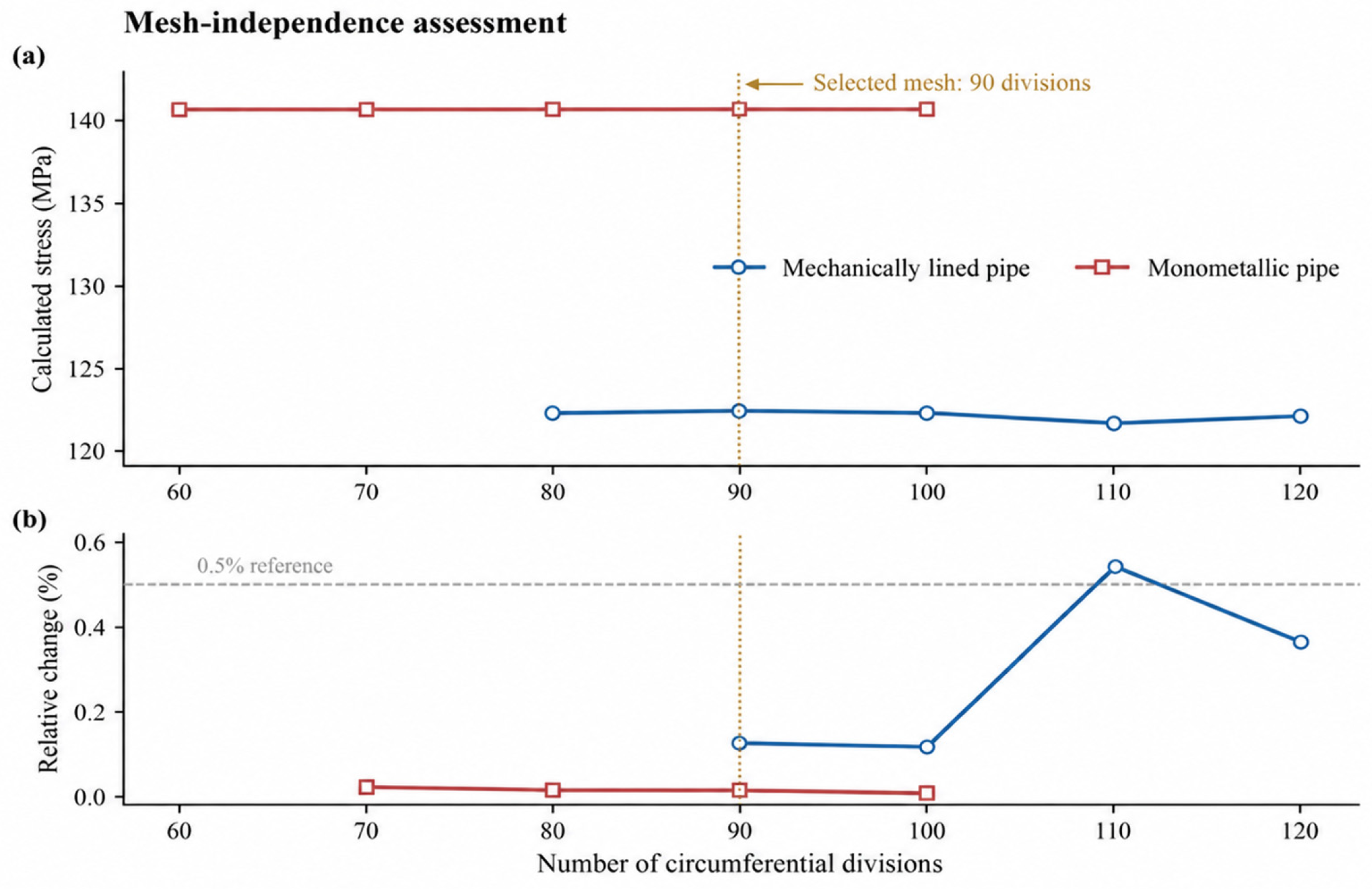
The circumferential mesh study reported stress changes of 0.014% for the monometallic pipe and 0.123% for the MLP at 90 circumferential divisions (Figure 1). These results support the selected circumferential discretization for the reported global stress measures.

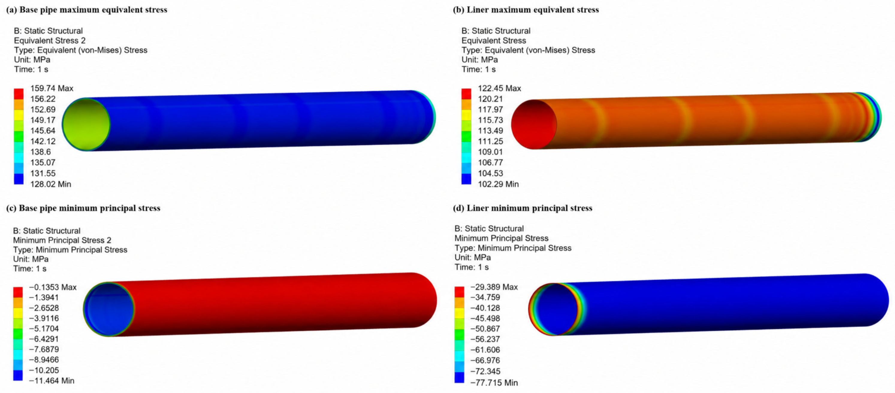
The baseline stress fields were inspected before scalar response extraction. Figure 2 maps equivalent and minimum principal stresses in the base pipe and liner, allowing the response locations and interlayer stress redistribution to be checked directly.

The base-pipe equivalent-stress field and the liner minimum-principal-stress field occupy different spatial regions (Figure 2). The former is used as the load-bearing strength response; the latter identifies local prebuckling compression requiring further nonlinear assessment.

As shown in Figure 2, the high-stress regions in the base pipe and liner differ spatially under interfacial constraint and bending, indicating layered load bearing and stress redistribution within the composite pipe. The maximum equivalent stress in the base pipe is used as a strength-response indicator for the load-bearing layer, whereas the liner minimum principal stress reflects the degree of local prebuckling compression on the compressive side. These two quantities are therefore adopted as response indices in the subsequent parametric analysis. The liner-stress index identifies conditions that require further verification; by itself, it does not establish wrinkling initiation.

2.4. Comparison with Field Inspection Data

Metal magnetic memory inspection data from a representative section of a gas-gathering branch pipeline in M Gas Field were used to evaluate the model’s ability to predict field stress responses. The finite element model was based on the representative field pipe section, with an outer diameter of 323.9 mm. The base pipe and liner were 12 mm and 3 mm thick, respectively. L360QS steel was used for the base pipe and MP35N for the liner; their mechanical properties are listed in

Table 2. Mechanical properties of the field-validation materials.

Material	Elastic Modulus, E (GPa)	Poisson’s Ratio, ν	Yield Strength, σy (MPa)
L360QS base pipe	200	0.30	360
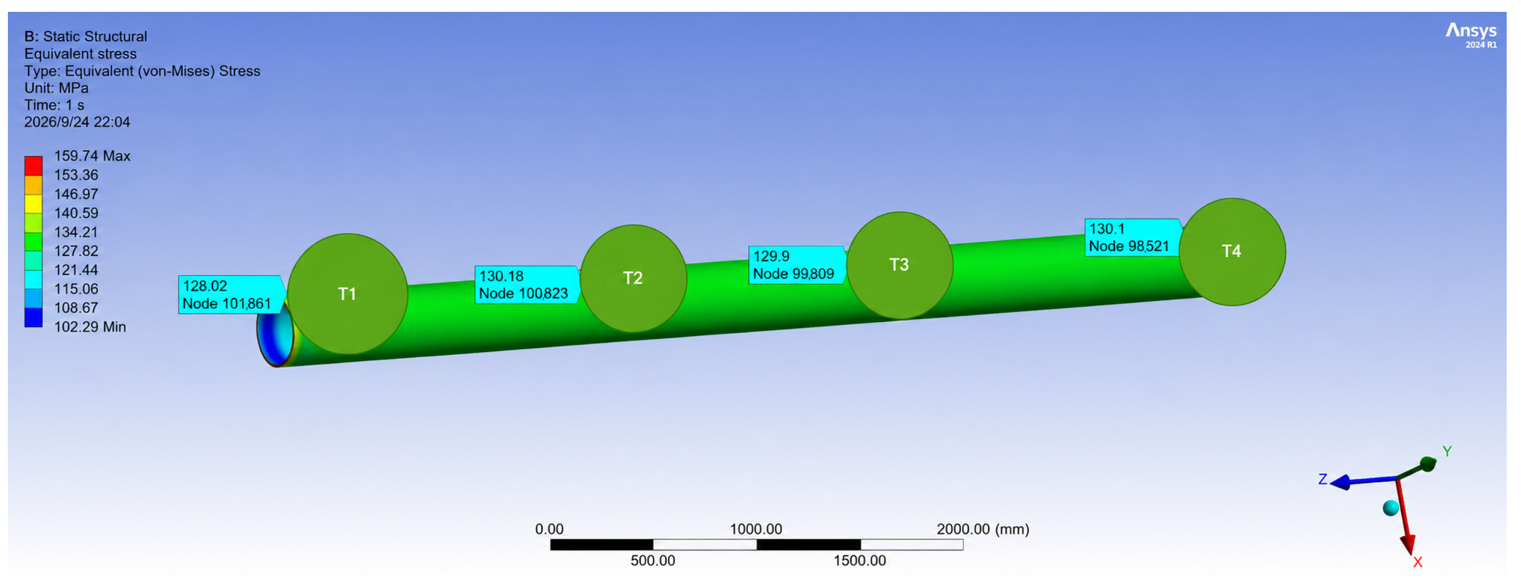
MP35N liner	210	0.31	400

. Four locations, designated T1–T4, were selected sequentially along the axial direction on the outer surface of the base pipe, as illustrated below. Measured from the left end shown in Figure 3, these locations were near the left end, in the left-hand interior, in the right-hand interior, and near the right end, respectively. Equivalent stresses were extracted at the corresponding nodes for comparison.

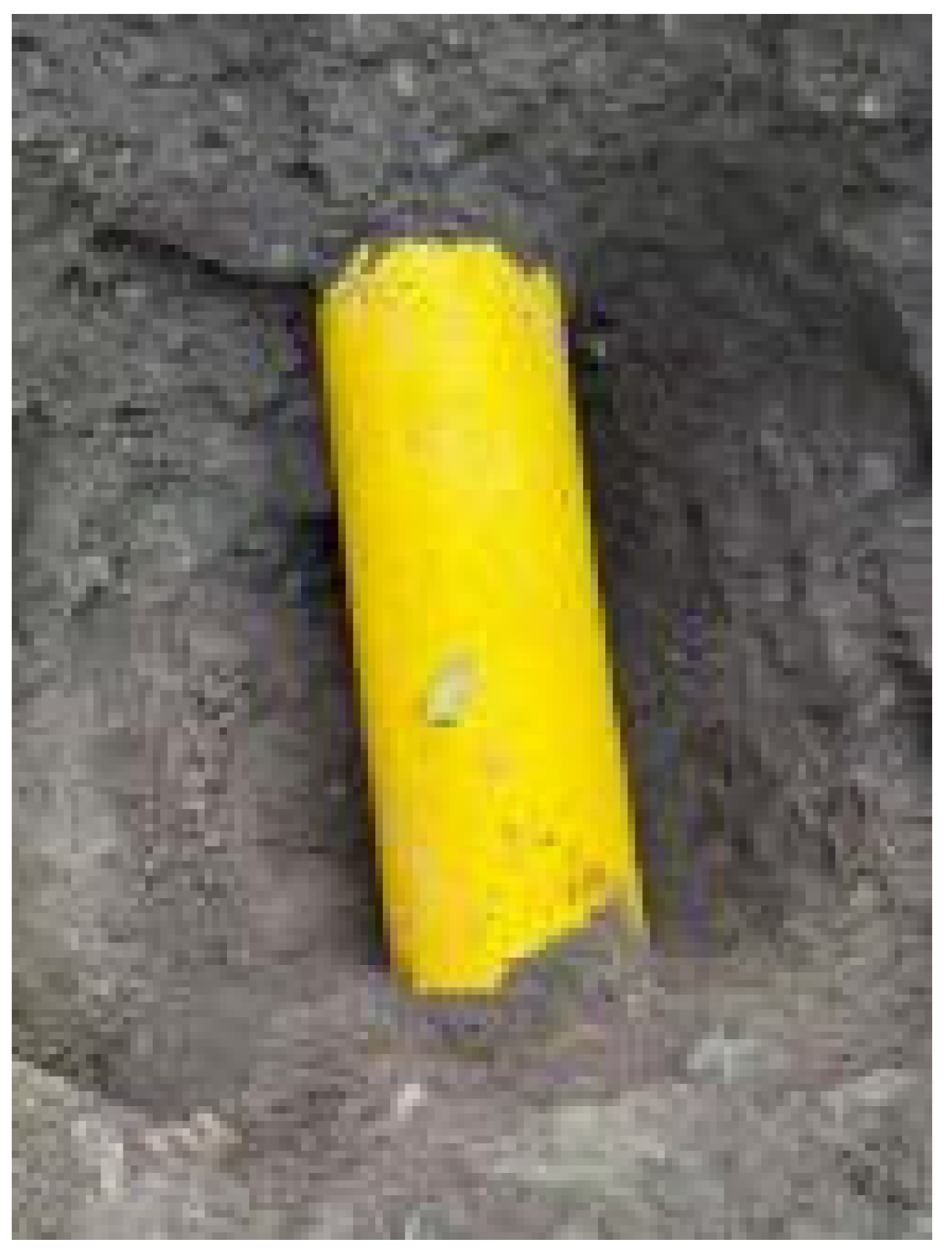
Field inspection was conducted using a JX-MTM metal magnetic memory instrument without excavation. This method requires no externally applied excitation and detects the magnetic leakage field generated by the pipe itself. Stress concentration regions are identified from features such as magnetic-field gradient extrema and zero-crossing points. Stress values are then inferred using a precalibrated relationship between the magnetic-field gradient and stress. The instrument was first subjected to a self-check and environmental calibration. The probe was subsequently held perpendicular to the ground and moved at a uniform speed along the pipeline. Magnetic signals were continuously acquired, and the inspection locations were recorded, As shown in Figure 4.

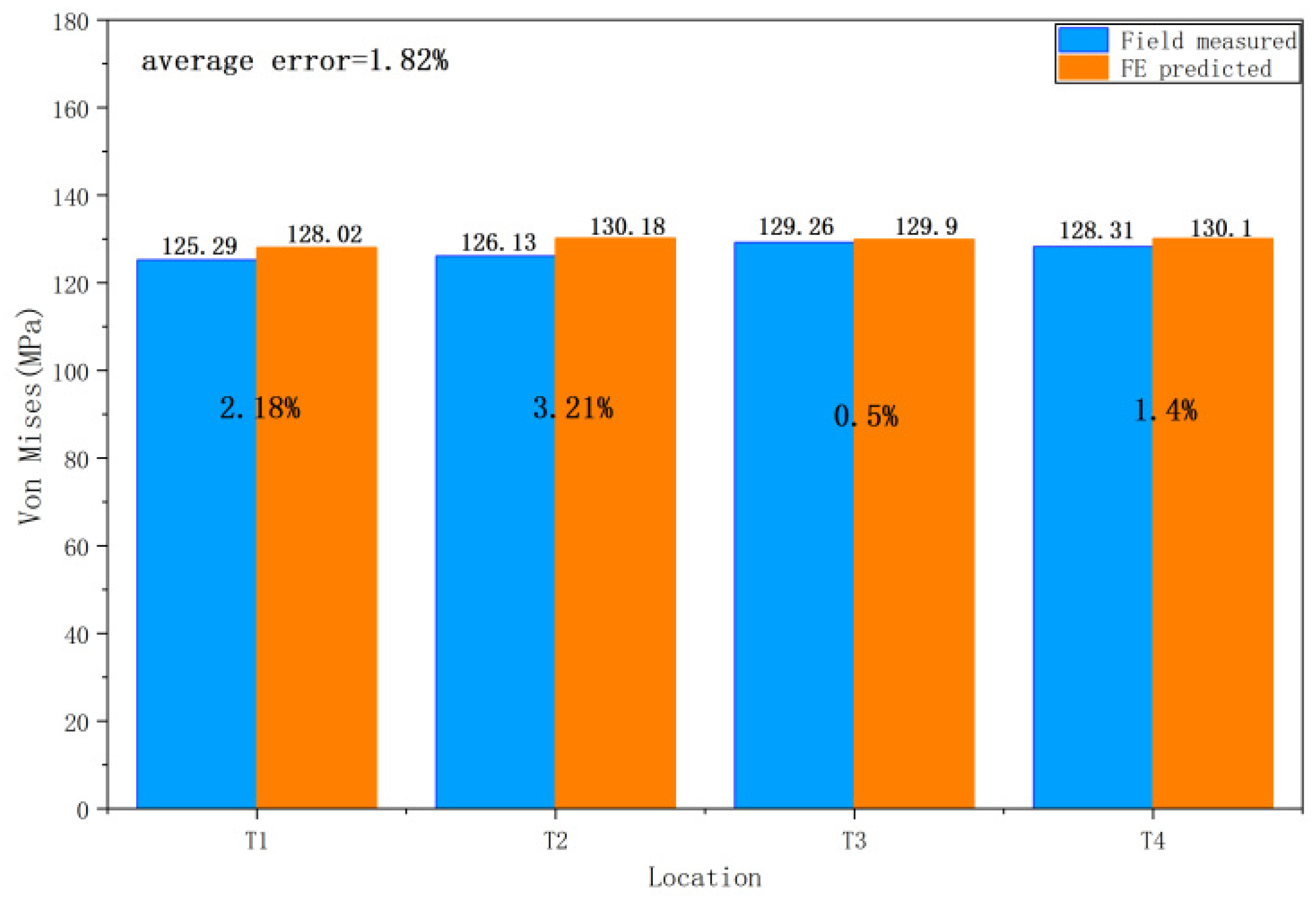
According to the inspection results, the stresses at T1, T2, T3, and T4 were 125.29, 126.13, 129.26, and 128.31 MPa, respectively. These four locations were selected for model validation. After confirming that consistent stress measures were used for simulation and inspection, the corresponding model outputs were extracted and compared point by point with the field values. As shown in Figure 5, The relative errors at the four locations were 2.18%, 3.21%, 0.50%, and 1.40%, respectively, all below 5%, with a mean relative error of 1.82%. The finite-element and field-derived stress values were consistent at the four selected locations of this representative pipe segment.

3. Comparison of Stress Responses Between Monometallic and Mechanically Lined Pipes

This section isolates the effects of pressure, temperature, liner thickness, diameter, and moment while holding the remaining variables fixed. Maximum von Mises stress is reported for the monometallic pipe and the MLP base pipe. Minimum principal stress is reported at the monometallic inner wall and in the liner. These measures describe load-bearing strength and local compression, respectively, within the stated parameter ranges. Each one-factor series uses its own reference case. The pressure series uses T = 150 °C, D = 323.9 mm, t = 3 mm, and M = 0. The temperature series uses P = 13 MPa, D = 323.9 mm, t = 3 mm, and M = 0. The thickness series uses P = 13 MPa, T = 150 °C, D = 323.9 mm, and M = 0. The diameter series uses P = 10 MPa, T = 80 °C, t = 3 mm, and M = 0. The moment series uses P = 13 MPa, T = 80 °C, D = 323.9 mm, and t = 3 mm. Section 4 uses a common baseline, so its local sensitivities should not be compared directly with these marginal trends.

3.1. Effect of Internal Pressure on Stress Response

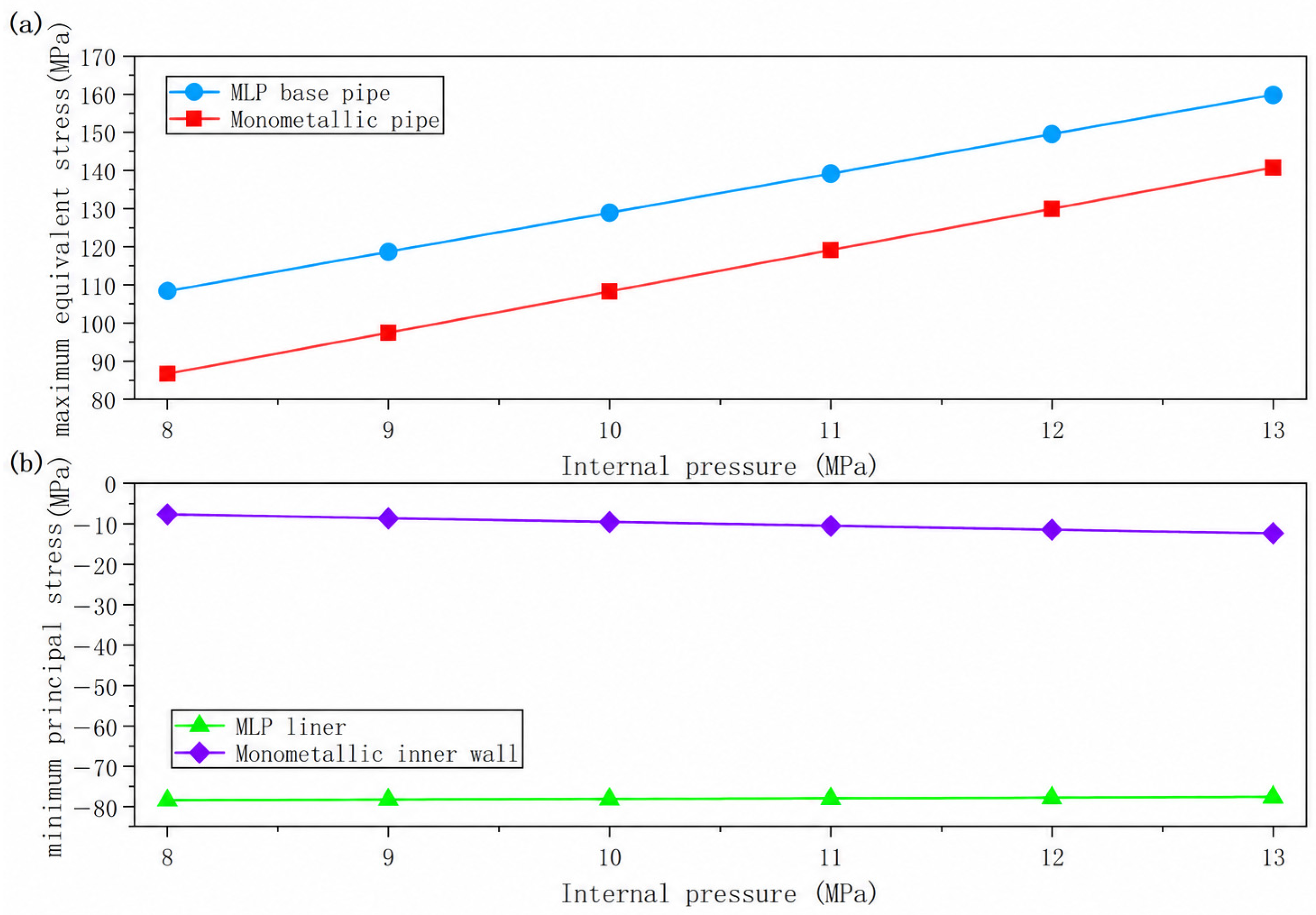
From 8 to 13 MPa, maximum equivalent stress increases approximately linearly in both structures (Figure 6a). The MLP base pipe remains more highly stressed than the monometallic pipe, while the two slopes are similar. At equal total wall thickness, the liner therefore changes load partitioning without materially changing the near-linear pressure dependence of this response.

The minimum-principal-stress responses differ more clearly (Figure 6b). Liner stress remains near −78 MPa, whereas the monometallic inner-wall stress decreases from about −7 to −12 MPa. Within this model and extraction location, pressure mainly changes the load-bearing equivalent stress and has only a small marginal effect on liner compression. Clarifying the mechanism would require the principal-stress components and their spatial evolution.

3.2. Effect of Temperature on Stress Response

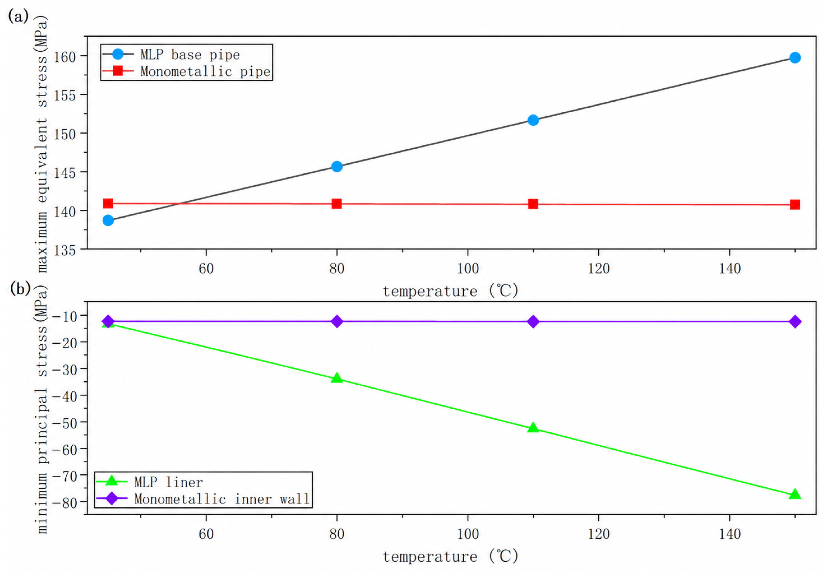
Between 45 and 150 °C, monometallic equivalent stress remains close to 141 MPa, while MLP base-pipe stress rises from about 139 to 159 MPa (Figure 7a). Their low-temperature values are similar, but they diverge as temperature increases. The additional thermal constraint is therefore carried mainly by the load-bearing layer of the composite pipe.

The contrast is stronger for minimum principal stress (Figure 7b). Monometallic inner-wall stress changes little, whereas liner stress falls from about −13 to −78 MPa. Thermal-expansion mismatch and interfacial constraint convert part of the free expansion into interlayer stress. Temperature consequently has little effect on the homogeneous pipe but increases both base-pipe equivalent stress and liner compression in the MLP.

3.3. Effect of Liner Thickness on Stress Response

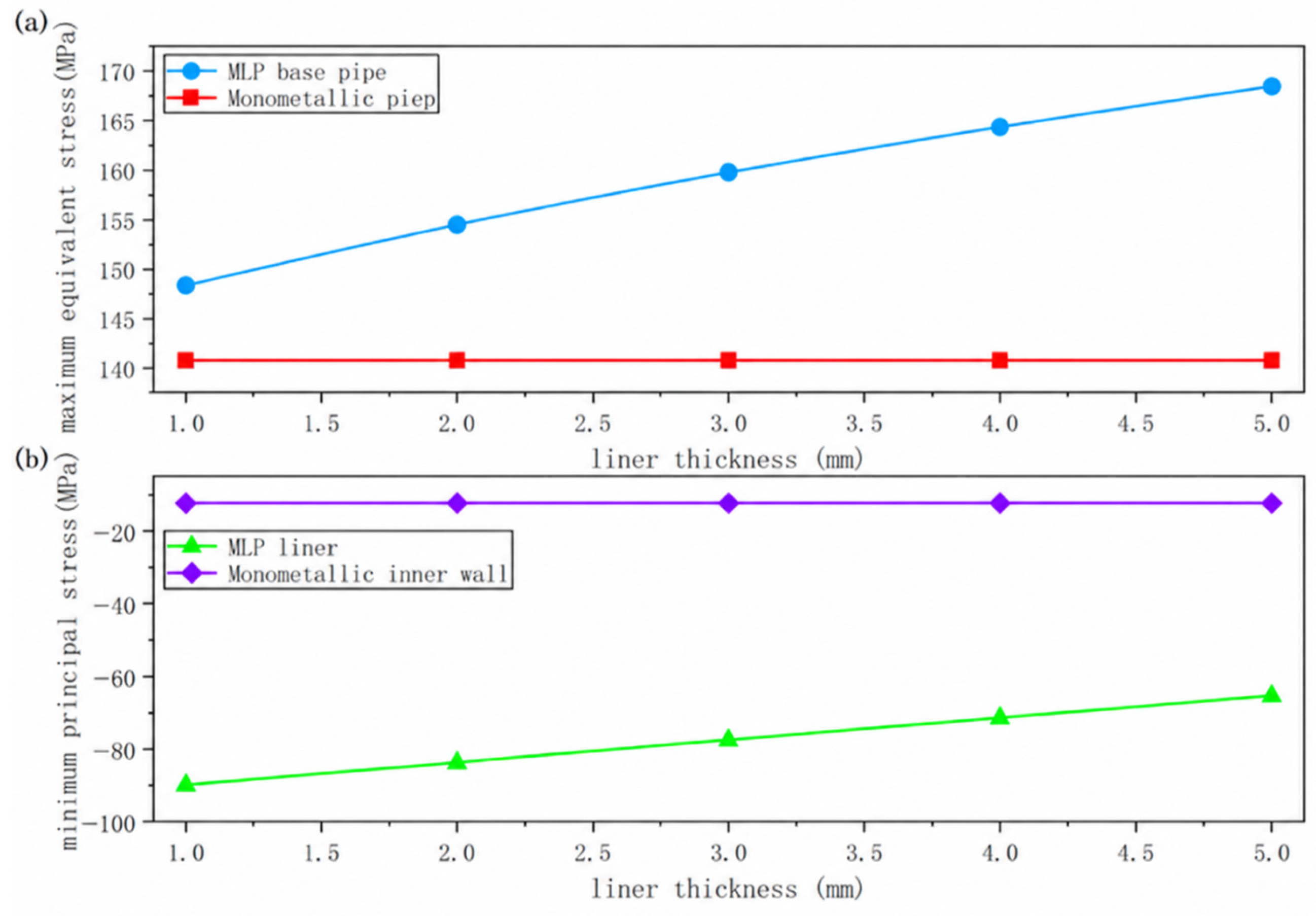
Increasing liner thickness from 1 to 5 mm raises base-pipe equivalent stress from about 148 to 168 MPa (Figure 8). Over the same range, liner minimum principal stress changes from about −90 to −66 MPa, reducing the compression magnitude. Both monometallic reference stresses remain constant because their geometry is unchanged.

These opposing trends arise from load redistribution at constant total wall thickness. A thicker liner carries more of the composite section and experiences less compression, but the thinner base pipe develops higher equivalent stress. Liner thickness must therefore be assessed against both liner stability and base-pipe strength.

3.4. Effect of Pipe Diameter on Stress Response

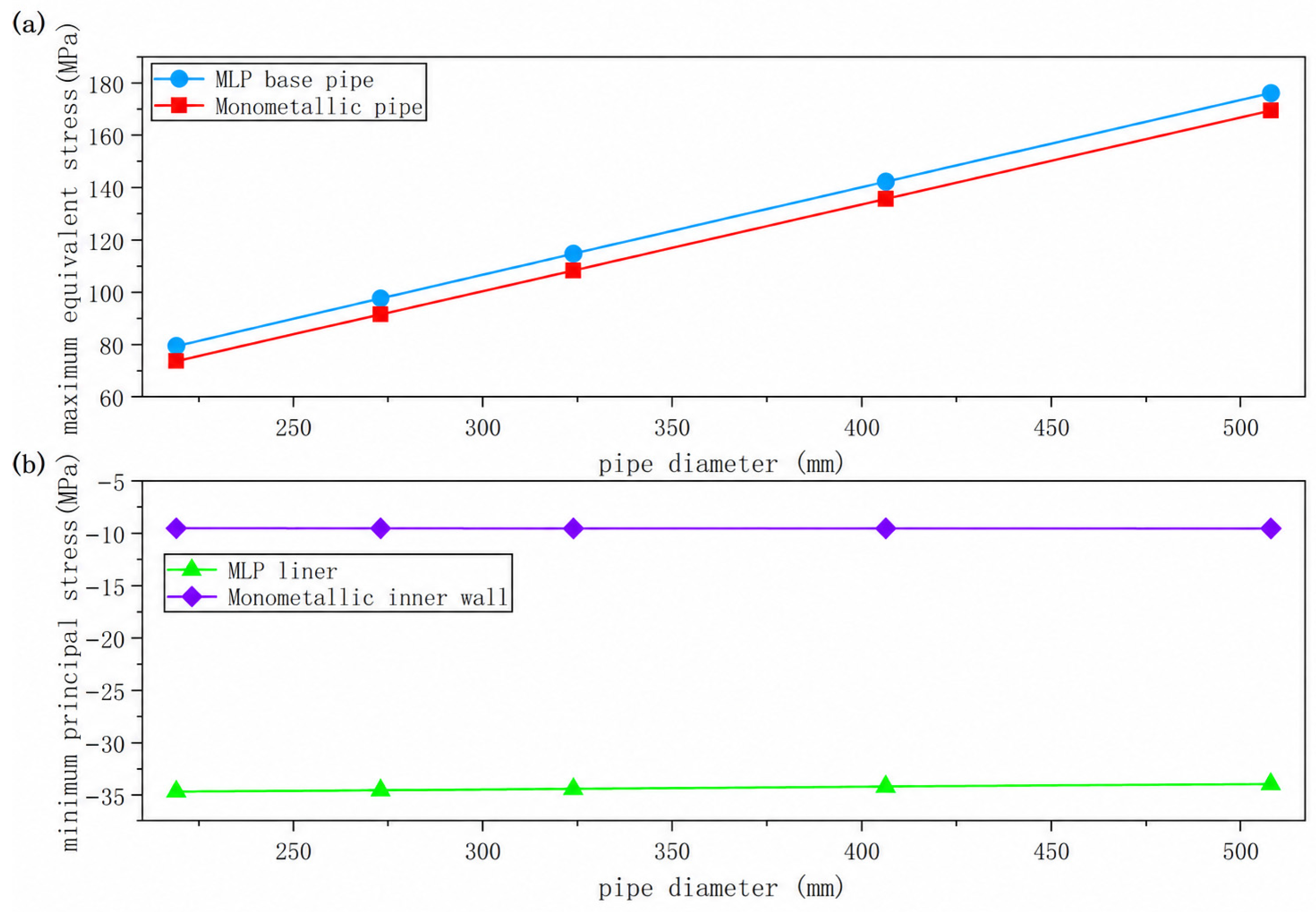
As diameter increases from about 220 to 510 mm, equivalent stress rises markedly and almost linearly in both structures (Figure 9a). The MLP base-pipe curve remains slightly above the monometallic curve. Minimum principal stress changes little with diameter (Figure 9b), remaining near −35 MPa in the liner and −9 MPa at the monometallic inner wall.

At fixed wall thickness and loading, a larger diameter increases the diameter-to-thickness ratio and changes the sectional stresses generated by pressure and bending. The pronounced size effect in equivalent stress is therefore expected. The present one-factor cases show no comparably strong diameter effect on minimum principal stress. This is a marginal trend under the stated controls; multivariable interactions with moment and temperature may differ.

3.5. Effect of Bending Moment on Stress Response

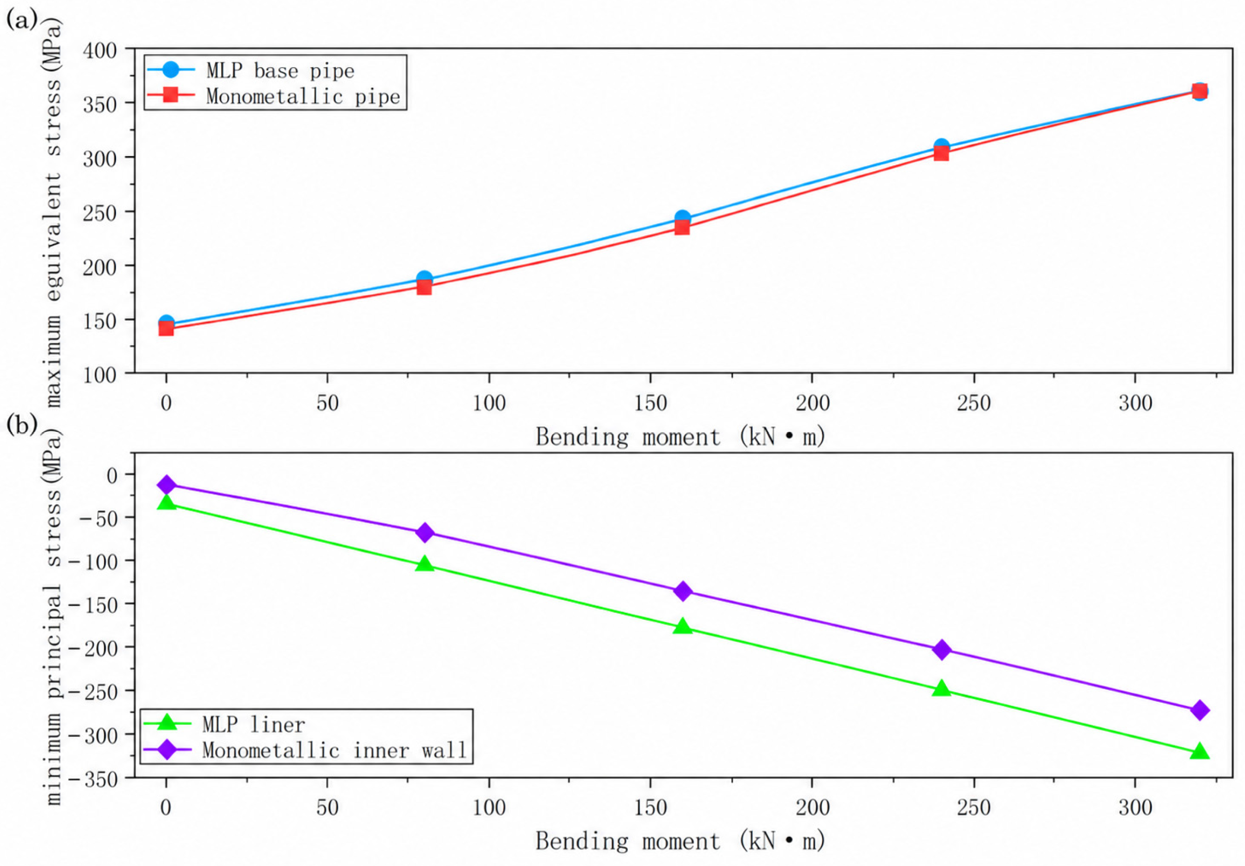
Bending amplifies both equivalent stress and compressive principal stress in the two structures (Figure 10). From 0 to 3.2 × 10⁸ N·mm, monometallic and MLP base-pipe equivalent stresses rise from about 140 to 360 MPa. The corresponding minimum principal stresses reach about −276 MPa at the monometallic inner wall and −321 MPa in the liner. Bending produces the largest stress changes among the five factors examined.

The two equivalent-stress curves remain close, but the MLP liner carries greater compressive principal stress throughout loading. The load-bearing layer thus governs the overall strength response, while local compression develops in the liner through bending and interfacial constraint. Both responses require attention where ground deformation adds bending. A dedicated nonlinear wrinkling analysis is still needed before liner stress can serve as an engineering criterion.

3.6. Overall Analysis

The one-factor cases reveal distinct load-transfer paths. Pressure and diameter mainly affect equivalent stress. Temperature has little influence on the monometallic pipe but increases both base-pipe stress and liner compression in the MLP. A thicker liner reduces its compression while increasing base-pipe stress, and bending produces the largest simultaneous change in both indices. Base-pipe strength and liner compression must therefore be evaluated together.

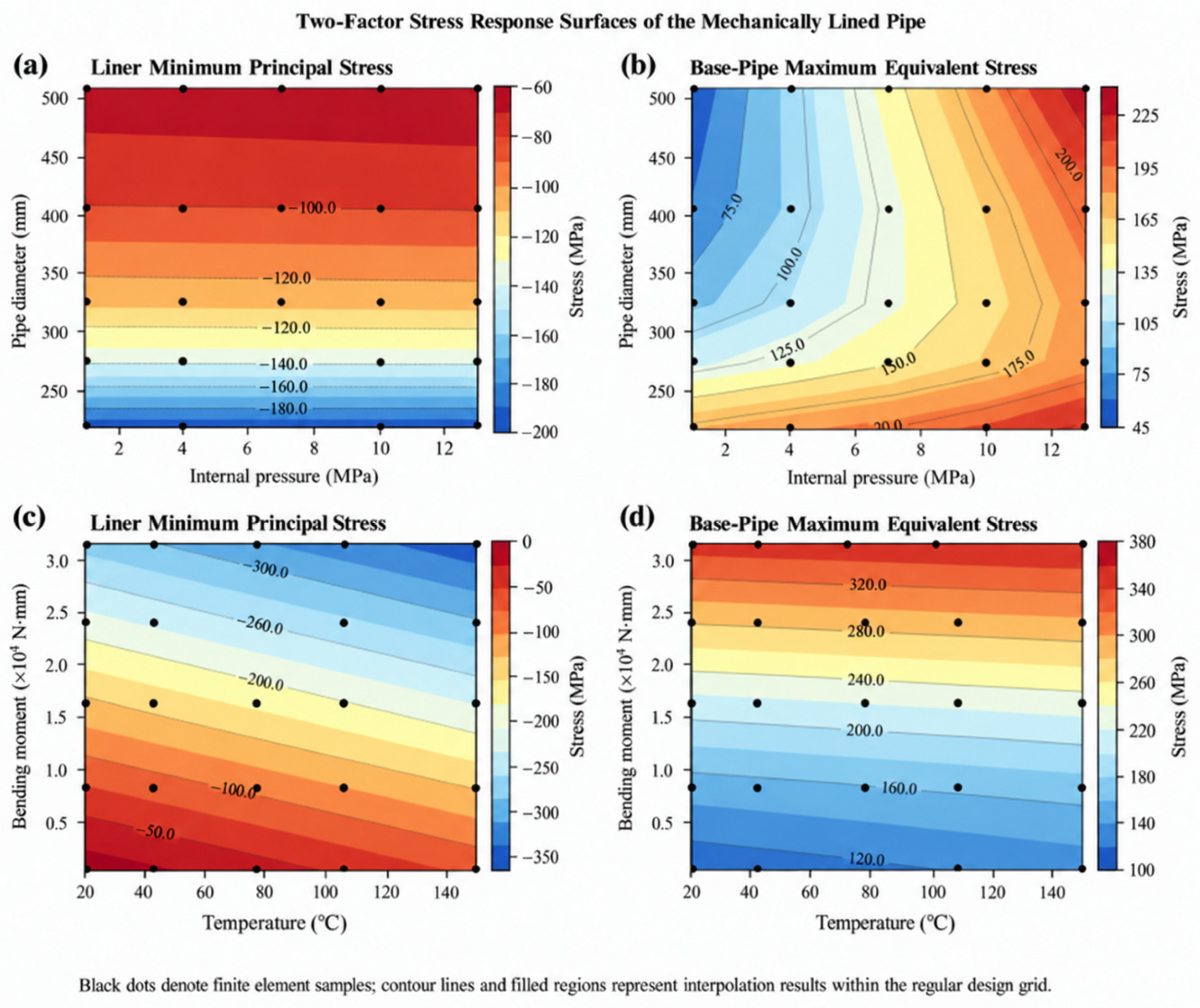
Because one-factor curves describe only marginal changes around different reference cases, Section 4 uses the broader set of 71 simulation records for normalized local sensitivity and two-factor response-surface analyses. These analyses compare local parameter influence and joint response trends but do not establish instability thresholds. All records used in Section 4 were computed with the remote-point configuration described in Section 2.1; the direct end-face displacement conditions used only for the four non-bending one-factor series were suppressed.

4. Parameter Sensitivity and Two-Factor Stress Responses of Mechanically Lined Pipes

Two complementary analyses are applied to the 71 simulation records. Signed normalized local sensitivities compare parameter influence near a specified baseline, while two-factor response surfaces map the computed stress gradients in pressure–diameter and temperature–moment planes.

4.1. One-Factor Local Sensitivity

One-factor local sensitivity is defined as the stress increment normalized by the magnitude of the baseline stress, divided by the relative parameter increment. The absolute value measures the local influence near the baseline condition, while the sign retains the physical direction of the stress increment. For minimum principal stress, a negative sensitivity therefore denotes evolution toward a more highly compressive state as the parameter increases. Because this measure depends on the baseline stress, reference loading condition, and perturbation magnitude, its ranking should not be equated directly with the raw stress increments reported in Section 3.

$$S_i={\displaystyle \frac{\Delta Y_i/\left|Y_0\right|}{\Delta X_i/X_{i,0}}}\times 100\%$$

(6)

where S_i is the normalized sensitivity coefficient of parameter X_i; X_i,0 and Y₀ are the baseline parameter and corresponding stress, respectively; and ΔX_i and ΔY are their increments relative to the baseline condition.

The baseline has 10 MPa pressure, 80 °C temperature, a 323.9 mm diameter, a 3 mm liner, and a 0.8 × 10⁸ N·mm moment. Each factor is varied independently while the remaining inputs stay at these values.

Table 3. Signed normalized local sensitivity coefficients and test levels.

Response	Parameter	Test Level 1	Test Level 2	Test Level 3	Test Level 4
Liner minimum principal stress	Internal pressure	1.21 1 MPa	1.21 4 MPa	1.21 7 MPa	1.21 13 MPa
Liner minimum principal stress	Temperature	−45.75 20 °C	−45.79 45 °C	−45.81 110 °C	−46.14 150 °C
Liner minimum principal stress	Pipe diameter	263.33 219.1 mm	184.05 273.1 mm	100.25 406.4 mm	72.51 508 mm
Liner minimum principal stress	Liner thickness	21.42 1 mm	19.82 2 mm	17.31 4 mm	16.27 5 mm
Liner minimum principal stress	Bending moment	−67.47 ≈0 N·mm	−68.02 1.6 × 108 N·mm	−68.02 2.4 × 108 N·mm	−68.02 3.2 × 108 N·mm
Base-pipe maximum equivalent stress	Internal pressure	51.21 1 MPa	55.37 4 MPa	58.51 7 MPa	60.62 13 MPa
Base-pipe maximum equivalent stress	Temperature	8.61 20 °C	8.69 45 °C	8.86 110 °C	8.96 150 °C
Base-pipe maximum equivalent stress	Pipe diameter	−107.15 219.1 mm	−35.55 273.1 mm	20.73 406.4 mm	35.88 508 mm
Base-pipe maximum equivalent stress	Liner thickness	−17.93 1 mm	−16.76 2 mm	−14.76 4 mm	−13.92 5 mm
Base-pipe maximum equivalent stress	Bending moment	27.52 ≈0 N·mm	37.75 1.6 × 108 N·mm	40.78 2.4 × 108 N·mm	42.20 3.2 × 108 N·mm

reports the resulting local sensitivities and the corresponding parameter levels.

At the specified baseline, the liner coefficient reaches 263.33% at D = 219.1 mm, a 32.36% decrease from the baseline diameter of 323.9 mm (Table 3). Across the four diameter levels, its magnitude (72.51–263.33%) exceeds that of the other tested factors. Bending moment and temperature have negative coefficients of approximately −68% and −46%, respectively, whereas pressure remains at 1.21%. These comparisons apply only to the listed perturbations.

For base-pipe equivalent stress, pressure coefficients range from 51.21% to 60.62%, while bending-moment coefficients range from 27.52% to 42.20% (Table 3). Diameter has the largest absolute coefficient at D = 219.1 mm (−107.15%) and changes sign across the listed levels; neither pressure nor moment is uniformly the most influential factor. Temperature coefficients remain below 9%, and liner-thickness coefficients range from −17.93% to −13.92%.

The test levels represent unequal changes relative to the baseline, so the coefficients characterize specific finite perturbations rather than identical percentage steps. The diameter response is also asymmetric. Table 3 therefore does not establish a single global ranking of the five variables or substitute for combined-loading analysis.

Within the tested levels, pipe diameter and bending moment affect both response measures, but their relative sensitivities depend on the level considered. Pressure has much larger normalized coefficients for base-pipe equivalent stress than for liner minimum principal stress, whereas temperature shows the opposite contrast. These response-specific patterns motivate the two-factor combinations examined next.

4.2. Two-Factor Coupled Stress Responses

Unlike Section 4.1, this section does not calculate the ratio of the relative change in stress to the relative change in a parameter. Instead, liner minimum principal stress and base-pipe maximum equivalent stress are used directly as the response variables. For any two-factor combination, these responses are written as σ_liner = f(X₁,X₂) and σ_base = g(X₁,X₂), where X₁ and X₂ are the inputs under consideration. Based on the one-factor results, the internal pressure–diameter and temperature–bending moment combinations represent geometry–pressure and thermal–bending coupling, respectively. Black points denote finite element samples, whereas contours and filled regions interpolate over the regular design grid. Color bars report stress in MPa. The surfaces describe trends only within the sampled domain; no extrapolation is performed beyond its boundaries.

In the pressure–diameter plane, liner-stress contours change mainly with diameter and only weakly with pressure (Figure 11a). Base-pipe equivalent stress responds to both inputs, and the curved contours indicate a joint effect that cannot be inferred from one-factor trends alone (Figure 11b).

Moment dominates both responses in the temperature–moment plane (Figure 11c,d). Higher temperature adds liner compression and a smaller increase in base-pipe equivalent stress. The highest temperature and moment consequently give the largest joint response within the sampled plane.

The four surfaces do not share the same stress gradients or high-response regions. This difference motivates separate empirical equations for liner compression and base-pipe equivalent stress, but it does not validate either response as a standalone failure criterion.

The two analyses answer different questions. Normalized local sensitivity compares individual perturbations near one baseline and is reported as a percentage. The response surfaces map stress in MPa while two inputs vary together. Their equations and color scales are therefore not interchangeable.

5. Exploratory Regression Equations and Independent Evaluation

5.1. Structured-Sample Regression Equations

This section examines the limitations of fitting a five-dimensional response from a structured one- and two-factor simulation dataset. Diameter D, bending moment M, pressure P, temperature T, and liner thickness t are used to fit descriptive equations for liner minimum principal stress and base-pipe maximum equivalent stress. The equations are neither probability-of-failure models nor wrinkle-initiation predictors, and they are not offered for engineering prediction.

The original dataset contains 71 finite element simulation records. After checking the consistency of parameter combinations, the stress results for duplicate conditions are verified and merged, yielding 53 unique parameter combinations for model development and internal cross-validation. In these development cases, the base-pipe thickness was fixed at 12 mm. A separate set of 22 multivariable finite element cases is reserved exclusively for independent evaluation and is not used to estimate or modify the regression coefficients.

Because the input variables differ substantially in their dimensions and orders of magnitude—particularly because bending moment is several orders of magnitude larger than the other parameters—each input is standardized before modeling:

$$z_i={\displaystyle \frac{x_i-{\mu }_i}{s_i}}$$

(7)

where x_i is the ith input variable, and μ_i and s_i are its mean and standard deviation in the modeling sample, respectively. The standardization parameters for all inputs are listed in

Table 4. Standardization parameters for the predictive-model inputs.

Parameter	Mean	Standard Deviation
Pipe diameter, D (mm)	334.372	70.778
Bending moment, M (N·mm)	1.1774 × 108	8.7365 × 107
Internal pressure, P (MPa)	8.585	3.276
Temperature, T (°C)	80.472	31.657
Liner thickness, t (mm)	3.000	0.434

.

A multiple linear model containing only the five first-order terms is first established. The results indicate that the linear model captures the overall trends, but the residuals still exhibit a structured distribution. The model terms are therefore progressively modified using cross-validation error as the criterion, in conjunction with the nonlinear characteristics and combined parameter effects identified in the preceding response analyses.

For the minimum principal stress in the liner, adding the quadratic pipe-diameter term markedly improves model accuracy, whereas further quadratic and interaction terms do not improve cross-validation performance. The resulting liner-stress empirical response equation is therefore expressed as

$${\sigma }_{\mathit{liner}}=-135.7024+39.2233z_D-77.9187z_M+0.5666z_P-18.8557z_r+2.8832z_t-9.8745{z_D}^2$$

(8)

For the maximum equivalent stress in the base pipe, quadratic terms for all parameters, the internal pressure–diameter interaction, and the bending moment–temperature interaction are added to the first-order terms, yielding:

$$\begin{array}{l}{\sigma }_{\mathit{base}}=171.4584-16.4743z_D+61.9475z_M+29.9300z_P+4.9648z_T-3.6419z_t\\ +10.7492{z_D}^2+5.3726{z_M}^2+1.0106{z_P}^2+0.1087{z_T}^2-0.0392{z_t}^2+9.7637z_P{z}_D-1.0291z_M{z}_T\end{array}$$

(9)

where z_D, z_M, z_P, z_T, and z_t are dimensionless variables standardized using Equation (7); the corresponding standardization parameters are provided in Table 4. Thus, the coefficients apply to the standardized variables in the present sample. Model inputs must first be transformed using the same means and standard deviations. Each coefficient represents a conditional effect after controlling for the other terms and should not be equated directly with a marginal one-factor trend.

5.2. Internal Cross-Validation of the Empirical Response Equations

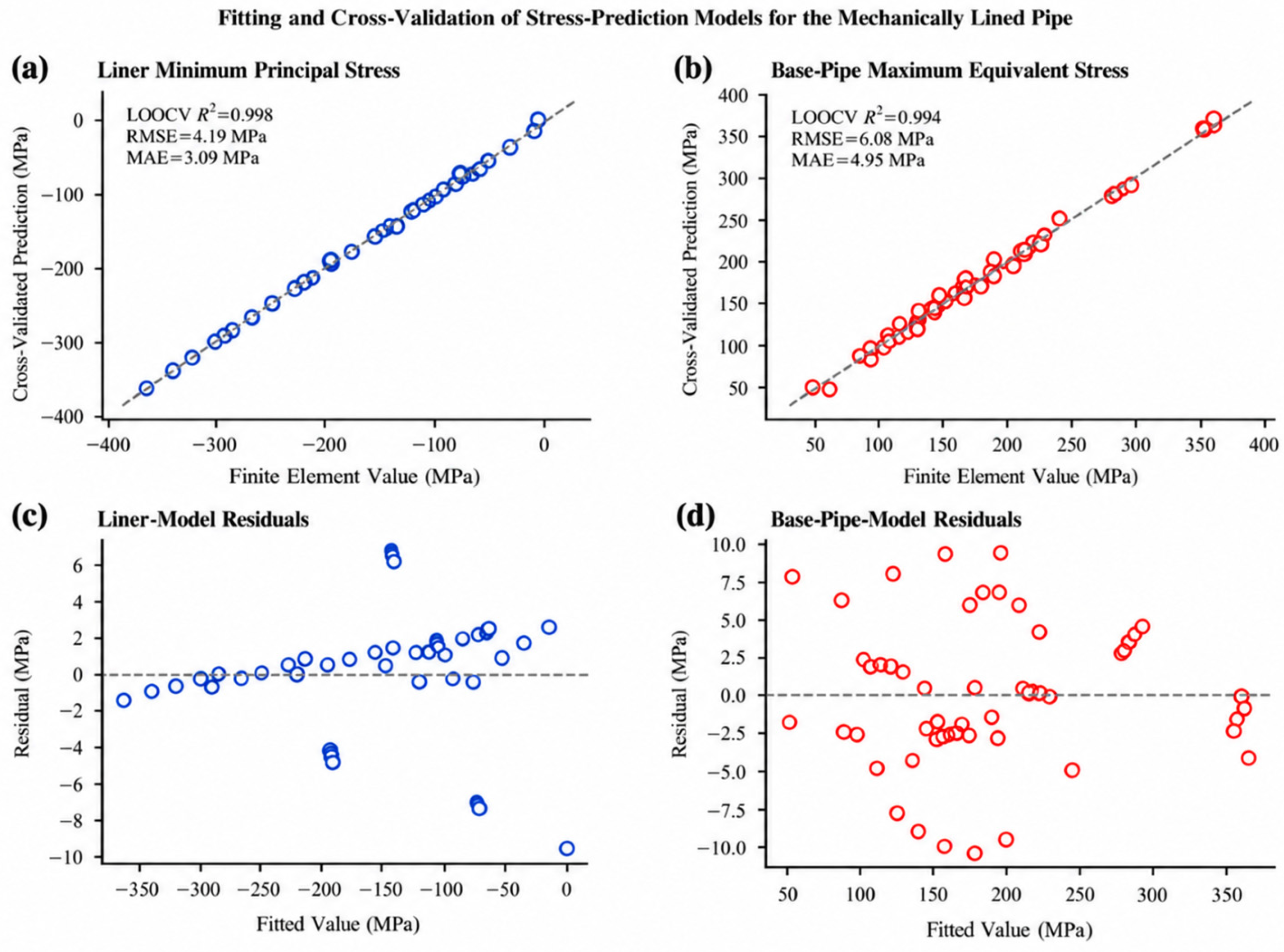
Leave-one-out cross-validation gives R² = 0.9976, RMSE = 4.19 MPa, and MAE = 3.09 MPa for the liner model, and R² = 0.9941, RMSE = 6.08 MPa, and MAE = 4.95 MPa for the base-pipe model. These values measure interpolation consistency within the structured development sample; they do not demonstrate generalization when all five variables change simultaneously.

Cross-validated predictions cluster around the 1:1 line without a clear monotonic residual trend (Figure 12). Several neighboring development cases nevertheless share fixed values for multiple inputs. Leave-one-out validation can therefore overstate performance for unsampled five-dimensional combinations.

Cross-validation therefore quantifies interpolation within the existing structured design rather than external predictive validity. The models remain unsuitable for extrapolation to extreme geological loads, material plastic evolution, interfacial damage, or untested multivariable combinations. Their broader applicability is assessed separately using the additional finite element cases.

5.3. Independent Evaluation on Finite-Element Cases

Twenty-two valid finite-element cases were used to evaluate the regression models. These cases were not included in the 53 unique combinations used for model fitting. Nine cases covered changes in outer diameter and internal pressure, eight covered changes in bending moment and temperature, and five covered changes in liner thickness. The base-pipe thickness was fixed at 12 mm. Predictions were calculated using the unchanged coefficients in Equations (8) and (9) and the standardization parameters in Table 4; no refitting or coefficient adjustment was performed.

For the liner minimum principal stress, the independent evaluation yielded an (R²) of 0.965, an RMSE of 11.54 MPa, an MAE of 5.22 MPa, and a mean absolute relative error of 3.79%. For the base-pipe maximum equivalent stress, the corresponding values were 0.986, 7.18 MPa, 4.55 MPa, and 2.77%. The regression equations captured the overall stress variation paths. Thus, the results support using the equations to estimate stress trends within the tested conditions.

5.4. Scope and Limitations

The stress trends reported in this study are conditional on the modeled geometry, assumed initial contact state, friction coefficient of μ = 0.20, open-ended pressure loading, and prescribed boundary conditions. The applied bending moment represents a structural loading condition rather than a coupled pipe–soil or landslide process. Consequently, the results describe stress redistribution under the investigated conditions; their transfer to other interface states, loading paths, or restraint conditions requires separate assessment.

6. Conclusions

(1) As pressure increased, equivalent stress rose approximately linearly in both pipes. The MLP base pipe carried higher equivalent stress; liner compression changed little, whereas the monometallic inner wall became slightly more compressive.

(2) Increasing temperature had little effect on monometallic-pipe stress but increased both base-pipe equivalent stress and liner compression in the MLP.

(3) At constant total wall thickness, a thicker liner reduced its compression but increased base-pipe equivalent stress. The monometallic reference was unchanged because it has no liner.

(4) In the non-bending one-factor diameter series, increasing diameter raised equivalent stress in both pipes, while the minimum principal stresses at the monometallic inner wall and in the MLP liner changed little.

(5) In the one-factor stress-response curves, bending moment produced the largest stress-change magnitudes among the five factors in both pipes. It increased equivalent stress and compression, with greater compressive stress in the MLP liner than at the monometallic inner wall.

(6) For the 22 finite-element cases, the unchanged regression equations yielded R² values of 0.965 for liner stress and 0.986 for base-pipe stress. They support stress-trend estimation under these conditions, but their accuracy for arbitrary five-factor combinations remains untested.