A Discrete Synthetic Benchmark for PCA-Ridge and Reference-Ray 3-D Velocity Reconstruction from First-Arrival Travel Times

Abstract

Learned methods for seismic travel-time tomography are usually compared with physics-based inversion on benchmarks whose representation and evaluation choices are left implicit. We show that the apparent workflow ordering depends materially on the declared representation choices, not only on the estimator. The benchmark reconstructs 3-D P-wave velocity from first-arrival travel times: 250 synthetic geological targets in five families, 384 source–receiver observations each, split 175/37/38 by target, with travel times from a Fast-Sweeping calculation on a 1.25 km grid and errors measured against analytic velocity at 2.5 km cell centers. With the corpus and endpoint fixed, the declared identifier-ordered principal component analysis ridge (PCA-ridge) workflow gives root-mean-square error of 0.353 km/s, geometry-canonical re-ordering with penalty reselection gives 0.310 km/s, and a cell-native parameterization gives 0.261 km/s, against 0.272 km/s for an intentionally non-equivalent reference-ray baseline (the cell-native paired interval spans zero); a small neural network in place of the linear map gives 0.352 km/s. The main reported comparison, retrospectively designated and descriptive, is a paired difference of +0.0816 km/s (95% percentile-bootstrap interval [+0.0492, +0.120] km/s) favoring the baseline. Benchmarks should therefore declare encoding and parameterization explicitly. Conclusions are conditional on the declared operator and representation, and establish no field-scale accuracy or universal method ranking.

1. Introduction

1.1. Seismic Travel-Time Reconstruction

Seismic tomography estimates spatial variations in subsurface velocity or slowness from indirect observations. In local-earthquake settings, first P-arrival times depend jointly on the source and receiver geometry, the propagation medium, and the forward approximation used to calculate the arrival [1,2,3]. The inverse problem is non-unique: resolution depends on acquisition coverage, parameterization, regularization, and noise, and multiple models can explain similar observations [4]. These properties make a reconstruction error meaningful only together with a precise statement of the target distribution, observation specification, evaluation domain, and independent experimental unit.

One physical reason for the dependence on coverage is simple to state. A first arrival is the earliest wave to reach the receiver, and by Fermat’s principle, it travels along a path of minimum travel time [5]. Its time therefore depends mainly on the velocity near that path, and parts of the model that no fastest path crosses are weakly constrained, whatever the reconstruction method. This is why coverage is part of the evaluation here, through the coverage-aware metrics of Section 2.10, which approximate those paths by reference-model rays.

The same considerations apply when the forward calculation and target are synthetic. Synthetic models make the generating velocity known and permit controlled ablations, but they do not provide field validation. In particular, a result obtained from repeated acquisition geometries of a small set of target models can overstate the number of independent geological examples. A model can also appear accurate because a target-space prior is restrictive, because the test structures are already represented in training, or because global metrics are dominated by weakly illuminated background cells. The present study treats these issues as part of the benchmark design rather than as post-processing details.

1.2. Related Work

Established travel-time tomography spans shooting, bending, perturbation, and grid-based forward calculations, and the choice of travel-time and ray-path approximation can affect both the data and the sensitivity matrix used in a subsequent inversion [5]. This study computes its labels with the Fast-Sweeping implementation of ttcrpy [6], following the formulation for eikonal equations analyzed by Zhao [7]. Two-point and bending ray tracing, which adjust a path between prescribed endpoints, provide relevant methodological context [8,9], and comparisons of three-dimensional ray-tracing methods show why the forward approximation must be reported explicitly [10]. The result is treated as a finite-grid approximation, and its specification is part of the benchmark definition (Section 2.4).

Learning-based travel-time tomography is itself an established research area. Earp and Curtis showed that the prior used to construct the training distribution affects both the inferred velocity and its uncertainty [11]. Supervised approaches have related source-location perturbations to lateral velocity variations under a linearized eikonal formulation [12] and predicted large-scale velocity models from first arrivals, with transfer learning [13,14]. Physics-informed approaches span joint P- and S-wave inversion, untrained-network reparameterization, spatial correlation constraints, and crosswell first-arrival inversion [15,16,17,18]. Comparative synthetic benchmarking of first-arrival methods also has precedent: the blind test of Zelt et al. compared fourteen reconstructions of one withheld 2-D near-surface model, produced by ten participants using eight inversion algorithms [19]. The specification declared here instead fixes a single learned estimator across a corpus of 3-D targets, so the two are complementary rather than directly comparable. OpenFWI demonstrates the value of multi-structure coverage and explicit generalization tests for full-waveform inversion, whose metrics are not directly comparable with the travel-time metrics reported here [20]. Reviews of machine learning in seismic velocity modeling identify recurring concerns about data distribution, validation, and transferability [21]; InversionNet is a representative method in that adjacent full-waveform setting [22], and a broader geoscience review discusses the same concerns [23]. Learned regularization and hybrid schemes form a further strand: dictionary learning within travel-time inversion as a locally sparse alternative to smoothness regularization [24], supervised descent learning of update directions from a training corpus [25], and deep learning combined with conventional first-arrival tomography, either supervised, with tomographic models as network inputs [26], or label-free, by optimizing dictionaries against a travel-time misfit [27]. Learning-based travel-time tomography is therefore not itself the novel contribution of the present study.

No individual component is novel either: PCA, ridge regression, finite-grid Fast-Sweeping, and supervised learning for tomography are all established, and the reference-ray path operator is a benchmark component rather than a new inversion algorithm. What this study contributes is a single declared benchmark specification in which the geological target identity, the independently sampled acquisition, the finite-grid observation operator, a non-learning comparator, the direct analytic cell-center evaluation endpoint, the target-level paired uncertainty procedure, and a checksum-pinned reproducibility record are specified jointly rather than separately, in keeping with the principles of findable, accessible, interoperable, and reusable research records [28]. Table S11 of Supplementary Materials Section S21 states each of these seven properties with the section and record where it can be checked, and Table S12 of Supplementary Materials Section S22 compares them against a representative subset of the studies cited above. The claim is not that any single property is new, nor that no earlier study has combined them, but that they are implemented jointly and auditably; the comparison is context for that contribution rather than evidence of uniqueness, and Supplementary Materials Section S22 states its scope and non-systematic nature.

1.3. Aim and Contributions

The aim is to test whether the ranking of reconstruction workflows on a benchmark reflects the methods alone or also the representation choices made in building it. We fix the target distribution, acquisition, forward calculation, estimator and statistical unit in advance, and ask what a fixed-length, identifier-ordered PCA-ridge model learns from synthetic first-arrival travel times. We then measure how the conclusions change with three choices: the order of observations in the feature vector, the target parameterization (nodes or cells), and the background prior given to the comparator (Section 2.9). Further sensitivities quantify the numerical-discrepancy scale of the declared finite-grid operator and check whether a nonlinear coefficient map changes the comparison.

The study does not ask what first-arrival data can support in general. Each feature position is indexed by a source and station identifier, not a fixed physical ray (Section 2.5), so the observation-content results are properties of this encoding. The paper is a benchmark study; it proposes no new architecture and no general ranking of machine-learning (ML) and tomographic methods.

The contributions are evaluative rather than algorithmic:

• A 250-target corpus of five parameterized geological families with exact target-hash checks and a deterministic target-atomic split of 175 training, 37 validation, and 38 test targets;
• A documented finite-grid Fast-Sweeping observation operator separated from the 2.5 km target grid, reported through a common direct analytic cell-center metric specification with target-level paired uncertainty;
• Controlled observation-information comparisons against a training-target mean prior and against a reference-model fixed-ray regularized path-operator baseline, together with a training-derived background-value substitution sensitivity under frozen regularization;
• Structure-aware, coverage-aware, family-resolved, and timing-noise diagnostics that make the benchmark’s limits visible alongside its main reported results;
• Sensitivities of the comparison to the observation encoding, the target parameterization and the coefficient map, each measured against the same baseline and endpoint.

The central empirical result is that the apparent ordering of workflows depends on declared representation choices, not only on the estimator; the benchmark makes these choices explicit and checkable. Supplementary Materials Table S12 sets its declared properties against three representative prior studies; what it adds is not a new component but the declaration, variation and joint reporting of the choices on which an ordering depends. All conclusions are restricted to the configured synthetic distribution and the declared finite-grid operator.

2. Materials and Methods

2.1. Study Design and Coordinate System

The benchmark uses a Cartesian volume of 100 km × 100 km × 30 km. Coordinates are expressed in kilometers, the surface is at z = 0, and positive z increases with depth. Station locations, earthquake hypocenters, analytic geological constructions, forward-grid nodes, target-grid nodes, and observation records use this same convention. The configured P-wave velocity range is 3.0–8.0 km/s.

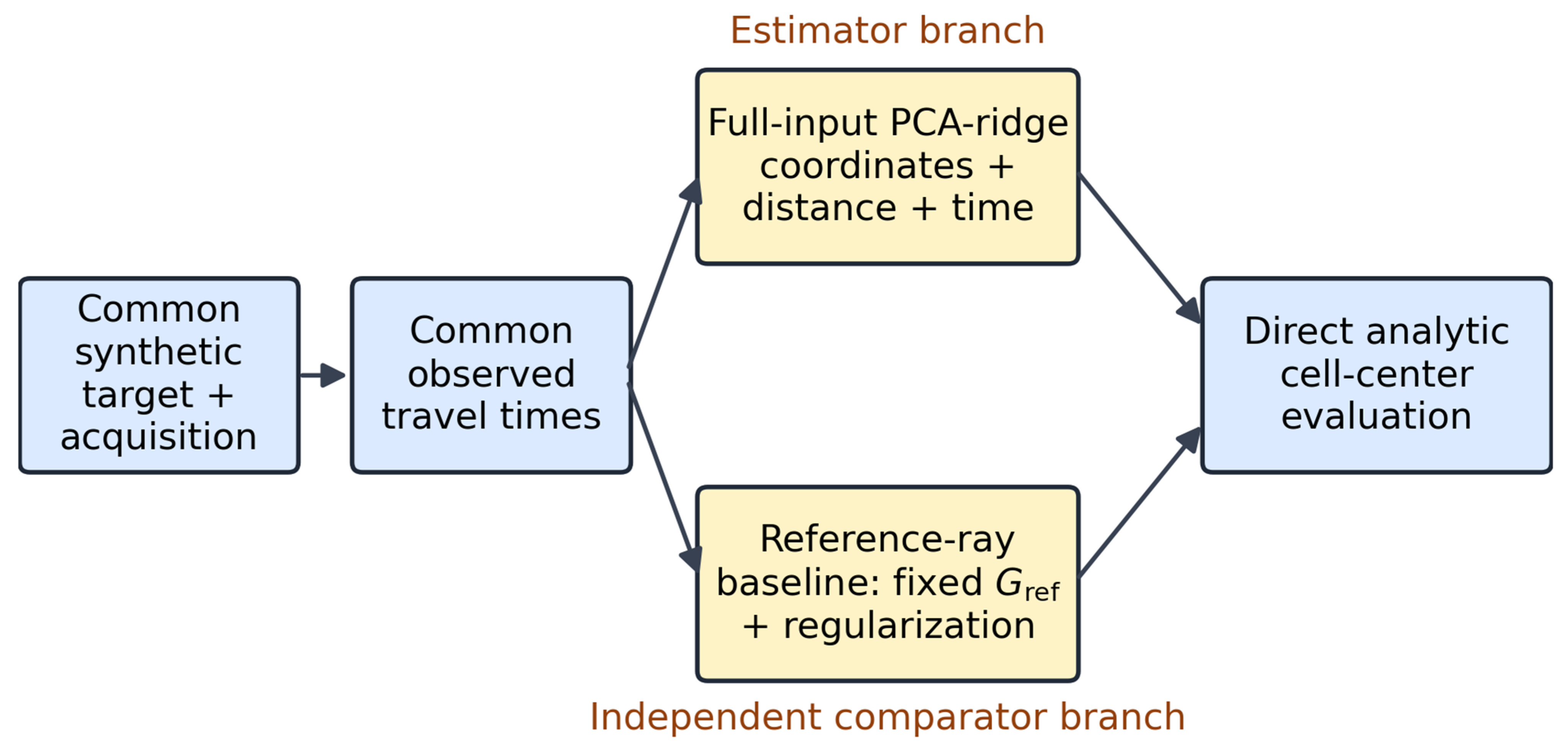
The branched benchmark workflow is summarized in Figure 1.

The analytic geological construction is evaluated independently on a fine forward grid for travel-time calculation and on the coarser reconstruction target grid for supervised reconstruction. The two grids are therefore not conflated: forward numerical resolution is not determined by the dimensionality of the PCA-ridge reconstruction.

2.2. Parameterized Geological Target Corpus

The production corpus contains five controlled families, each sampled from bounded parameter distributions rather than from a fixed set of repeated variants, chosen to create interpretable structural variation while remaining compatible with the target grid.

Table 1. Benchmark design and geological parameter ranges. Ranges are the configured sampling intervals. Each family contributes 50 unique targets. Contrasts and body velocities are bounded so that generated values remain in the configured physical range.

Family	Targets	Main Sampled Parameters	Configured Range or Constraint
Layered	50	Five-layer velocities and ordered boundaries	Initial velocity 3.8–4.2 km/s; minimum layer thickness 4.0 km; increments 0.45–0.75 km/s
Block anomaly	50	Center, dimensions, signed velocity contrast	Center x,y: 25–75 km, z: 8–22 km; x,y size 10–20 km; z size 7–14 km; absolute contrast 0.35–0.60 km/s
Faulted	50	Fault position, strike, dip, side offset	Position x,y: 25–75 km; strike 0–180°; dip 65–85°; absolute offset 0.25–0.50 km/s
Salt dome	50	Center, radii, internal velocity	Center x,y: 25–75 km, z: 8–14 km; horizontal radii 7.5–15 km; vertical radius 4.5–7 km; body velocity 5.8–7.6 km/s
Dyke intrusion	50	Center, strike, length, width, depth interval, internal velocity	Center x,y: 25–75 km; strike 0–180°; length 30–55 km; width 7.5–15 km; top depth 4–8 km; bottom depth 20–28 km; body velocity 6.2–7.8 km/s

summarizes the production ranges; the complete realized parameter registry is retained with the evidence package.

Layered targets contain five ordered layers with thickness constraints that prevent very thin layers from dominating the 2.5 km target representation, and block, salt-dome, and dyke dimensions are sampled so that important bodies span multiple target-grid intervals where possible. Faults remain sharp synthetic interfaces. A single parameterized generator constructs every target, sampling the family parameters from the ranges in Table 1 and evaluating the resulting analytic velocity model on the target grid.

For each target, the generator records the family, all sampled physical parameters, an analytic-model seed, the target-grid artifact, the forward-grid configuration, and a canonical 256-bit Secure Hash Algorithm (SHA-256) digest of the target velocity vector, whose byte serialization is defined in Supplementary Materials Section S1. Exact duplicate hashes are rejected during generation, while near-neighbor models are retained when physically valid; target proximity is reported as a diagnostic in Section 3.1 and Supplementary Materials Table S2 rather than used as a rejection threshold.

2.3. Acquisition Design and Observation Records

The production benchmark uses one acquisition realization per unique geological target. Each realization contains 16 stations at the surface and 24 synthetic earthquake sources, producing 384 source–receiver observations. Station and source coordinates are generated from distributions that are identical across families, their acquisition seeds are independent of the geological-model seeds, and the complete coordinates and seeds are stored in the target registry.

Each observation records the source coordinates, receiver coordinates, Euclidean source–receiver distance, travel time, target identity, acquisition identity, solver configuration, and finite-value status. Stations are sampled uniformly in x,y ∈ (5, 95) km at z = 0 and sources are sampled uniformly in x,y ∈ (5, 95) km and z ∈ (5, 25) km, with no minimum station–station, source–source, or source–station separation imposed. The final corpus contains 250 acquisition cases and 96,000 production observations, whose offset and travel-time distributions are summarized in Supplementary Materials Section S1.

Because there is one acquisition realization per target, the acquisition case and geological target have a one-to-one file-level correspondence, and the independent statistical unit is nevertheless defined as the unique geological target. The benchmark therefore evaluates performance over the configured joint target-and-acquisition distribution: it does not estimate within-target variability across repeated acquisition geometries or acquisition invariance, and target and acquisition effects cannot be decomposed within this design.

One consequence concerns the method comparison. Each target is observed through a single random acquisition draw, so a target whose sources and stations happen to sample its structure poorly can score badly for reasons unrelated to its geology. Both workflows are evaluated on the same draw for each target, so the draw is not itself a difference between them. If one workflow is more sensitive to poor coverage than the other, however, part of the paired difference is attributable to acquisition sampling rather than to geological structure, and neither its size nor its sign can be estimated here; the coverage-threshold diagnostic of Section 3.5 is only a partial check.

2.4. Authoritative Finite-Grid Forward Calculation

Travel-time labels are generated with ttcrpy==1.4.2 using its three-dimensional rectilinear-grid Fast-Sweeping Method (FSM). The fixed configuration uses tt_from_rp=False, node-centered velocity sampled directly from the analytic geological construction, and a 1.25 km × 1.25 km × 1.25 km forward-grid spacing. Source and receiver coordinates are passed at their saved continuous coordinates without project-side snapping, under the off-node conventions of the pinned implementation stated in Supplementary Materials Section S2 and in records/forward_solver_endpoint_contract.md. No ray paths are required for label generation.

The velocity field is evaluated at the nodes of an 81 × 81 × 25 forward grid. The package solves a discretized finite-grid travel-time problem; it is not used here to assert continuum-exact travel times, exact ray paths, or globally exact first arrivals. We call the labels a documented finite-grid 3-D Fast-Sweeping first-arrival approximation. Ray paths and path lengths, when produced for diagnostics or the reference-ray comparison, are not full-input PCA-ridge features.

Numerical checks included an analytical layered control, a finite heterogeneous refinement diagnostic, and a grid-aligned comparison with an independent finite-grid implementation. At 1.25 km spacing, the layered control had a mean absolute error of 0.030 s in the reported test, while the independent comparison had a mean absolute difference of 0.069 s (95th percentile of 0.100 s) over 15 comparable pairs. A separate grid-refinement audit compares the adopted 1.25 km grid with a 2.5 km grid over the full predeclared list of eight source–receiver geometries per family (forty pairs); Section 3.5 and Supplementary Materials Section S24 report it, and it is the least favorable of the three: finite-grid numerical discrepancies can be comparable to small structural signals, and for some geometries they exceed them. These checks indicate the numerical-discrepancy scale of the adopted operator rather than constituting a complete continuum convergence study. The benchmark is therefore defined as a discrete-operator benchmark, with physical interpretation conditional on the declared discretization and not extended to continuum-exact or field-scale forward accuracy.

Every travel time in the benchmark, for training, validation and test targets alike, comes from this one solver configuration, as do the reference times t_FSM(s₀) of Equation (3) in Section 2.9. Any systematic error of that configuration is therefore shared by all targets and by both workflows, and it is largely invisible from inside the benchmark: PCA-ridge is fitted and tested on observations from the same solver, and the reference-ray residual subtracts reference times from the same solver. Sharing the error does not make it neutral between the workflows, because they use the operator differently, as Section 4.4 discusses. The independent-solver comparison over 15 pairs, summarized by family in Supplementary Materials Table S6, and the refinement audit over 40 pairs described in Section 3.5, whose original 15 are listed in Supplementary Materials Table S9, indicate the size of this dependence but do not remove it. Whether the results hold for travel times from a different solver is not tested here.

The forward model is deliberately separate from the reconstruction target: the target field is evaluated on a 41 × 41 × 13 node-centered grid with 2.5 km cubic spacing, which prevents the output resolution of the learning problem from being treated as a validation of the forward physics. Supplementary Materials Section S2 states the forward endpoint and the target-truth convention in full.

2.5. Target Grid and Supervised Representation

The reconstruction target is the absolute P-wave velocity at 21,853 nodes (41 × 41 × 13). Nodes are flattened in x-fastest order, as stated in Supplementary Materials Section S2.

The declared identifier-ordered full-input observation vector contains, for each of the 384 observations, source (x,y,z), receiver (x,y,z), Euclidean source–receiver distance, and travel time. The rows are sorted deterministically by source identifier, station identifier, and observation identifier. The case-level vector therefore contains 3072 values (384 × 8). Position (j) in this vector denotes the same source and station identifier index within a case, not a physically fixed ray geometry across targets, because the acquisition coordinates are independently redrawn. The representation is therefore fixed-length and order-dependent rather than permutation-invariant or geometry-canonicalized. This encoding is retained because it was fixed before any test outcome was examined, not because it is physically preferred; Section 3.3 reports what changes when the same information is reordered geometrically. In the travel-time-only variant, the entries do not carry explicit geometry; in the full-input variant, coordinates are present but the linear estimator still acts on the ordered vector. The supervised sample is the complete case, not an independent velocity target for each source–receiver row.

The true-model ray path and its length are not included in the declared identifier-ordered full-input representation. They are privileged diagnostic quantities because they depend on the unknown target model. No geological-family label is supplied to the deployable variants.

2.6. Target-Atomic Splitting and Leakage Control

The split is defined before PCA fitting and model selection by sorting (family, target hash) within family and assigning deterministic contiguous groups. It contains 175 training, 37 validation, and 38 test targets, with family balance fixed by the production design: block anomaly 35/8/7, dyke intrusion 35/7/8, faulted 35/7/8, layered 35/8/7, and salt dome 35/7/8 (train/validation/test). Every target appears exactly once, every target hash is unique, and no hash crosses split boundaries. The split manifest was fixed before model fitting and was not changed in response to test performance.

This target-level split prevents a target from appearing in multiple splits through different acquisition geometries, and the integrity checks found no exact target-hash overlap across the three splits. It does not imply that nearby parameterized fields are absent: valid near-neighbor targets were retained, and the distance from each held-out target to its nearest training target is reported in Section 3.1 and Supplementary Materials Table S2, against the nearest-neighbor distances within the training set itself, rather than used as a rejection threshold. The centered 175 × 21,853 training matrix has numerical rank 151 against a maximum possible centered rank of 174, under the singular-value criterion stated in Supplementary Materials Section S1.

Target-atomic splitting removes one specific form of leakage, the same target reaching training and test through different records, and nothing more. The held-out targets are drawn from the same five families and the same generator parameter ranges as the training targets, so the test set measures performance within the configured target distribution. It does not measure generalization to structures outside that distribution, to other families, or to field conditions; the leave-one-family-out diagnostic described in Section 2.12 is the analysis here that holds out whole families. A test score on this benchmark is therefore an in-distribution score, not a simulation of deployment on new geology.

The split defines the independent unit for primary uncertainty: one unique geological target. If future versions include multiple acquisitions per target, case-level metrics must first be aggregated within target before resampling or inferential comparison.

2.7. PCA-Ridge Reconstruction and Model Selection

Principal component analysis (PCA) is used to represent the target-space prior [29]. Let y be a node-centered target vector, $\overline{\mathit{y}}$ the training-target mean, and u_k the principal directions estimated from training targets only. A K-component reconstruction is

$$\widehat{\mathit{y}}=\overline{\mathit{y}}+{\displaystyle \sum _{k=1}^K}{\widehat{c}}_k{\mathit{u}}_k,$$

(1)

where ${\widehat{c}}_k$ are predicted coefficients. Observation features are standardized column-wise over the fixed-length case feature matrix using training-case statistics only, and the coefficient map is fit using either a minimum-norm linear regression or ridge regression [30]. The reconstructed node vector is clipped element-wise to the configured 3.0–8.0 km/s range before the primary node-to-cell conversion. For a clipped node field ${\widehat{v}}_{i,j,k}^{node}$, the primary prediction cell is

$${\widehat{v}}_{i,j,k}^{\mathrm{c}\mathrm{e}\mathrm{l}\mathrm{l}}={\displaystyle \frac{1}{8}}{\displaystyle \sum _{a=0}^1}{\displaystyle \sum _{b=0}^1}{\displaystyle \sum _{c=0}^1}{\widehat{v}}_{i+a,j+b,k+c}^{\mathrm{n}\mathrm{o}\mathrm{d}\mathrm{e}},\hspace{1em}0\le i<40,0\le j<40,0\le k<12.$$

(2)

Thus, the prediction shape changes from 41 × 41 × 13 to 40 × 40 × 12 by eight-corner arithmetic averaging, with no second cell-level clipping step, and this transform is distinct from the direct analytic truth field defined below.

Validation selected PCA-ridge with K = 1 and α_ridge = 1000, whether scored by mean node root-mean-square error (RMSE) or against direct analytic cell-center truth over the same node-native candidate grid. That configuration was fixed before evaluation on the 38 test targets and held fixed for the original observation-control ablations, which were not independently retuned. The selected K = 1 is at the lower boundary of the component grid, whereas α_ridge = 1000 is interior to the ridge grid; the candidate-grid boundary observation therefore concerns K, and neither parameter is interpreted as globally optimal outside the tested candidate set.

A separate cell-native sensitivity fits the same observation representation to direct analytic cell-center target vectors and is selected independently on validation; its test result is not substituted for the node-native declared workflow. Cell-native predictions are clipped element-wise to the configured 3.0–8.0 km/s range before direct-cell evaluation. A training-only cell-PCA oracle curve accompanies it as a representation diagnostic that uses no test information for selection and is not an achievable prediction. Supplementary Materials Section S3 gives the candidate grids, the selection record, and both definitions in full.

Model selection here is exploratory. The declared full-input configuration was selected from 110 validation candidates: eleven component counts, each fitted by minimum-norm regression or by ridge regression at one of nine penalties from 10⁻⁴ to 10⁴. Every full-training-set validation search on the full-input features selected K = 1, the first value of the component grid, including the node-native and cell-native workflows, the geometry-canonical ordering of Section 3.3 and the network sensitivity described below; the independently tuned travel-time-only search selected K = 32. The selected penalty depended on the observation ordering, α_ridge = 1000 for the identifier ordering against 100 for the geometry-canonical ordering. The validation score of a configuration chosen in this way is an optimistic estimate of its performance. Each selected configuration was scored on the test targets once, after selection, so its test score carries no selection optimism; the decision to run and report further workflows was, however, made with earlier test results known. The selected values should therefore be read as the outcome of an exploratory search rather than as settings known to be optimal.

A neural-network sensitivity changes only the coefficient map. The ridge map from the standardized observation vector to the PCA coefficients is replaced by a small neural network with one hidden layer: tanh activation; 16 or 64 neurons in the hidden layer; weight penalty 0.1, 10 or 1000; training for a fixed 1000 epochs; and five networks averaged per configuration. Everything else is unchanged: the split, features, training-only PCA and component grid, clipping, node-to-cell conversion and validation-only selection. The network, its candidate grid and its selection rule were fixed in a written protocol, deposited with the records, before the network was run on any data of this benchmark, although the test results of the other workflows were already known. Nonlinear coefficient maps, including a network of this kind, had been used during development on earlier and smaller corpora that are not part of this benchmark; none had been run on this benchmark before the protocol was fixed. Supplementary Materials Section S27 states the protocol in full.

2.8. Observation-Information Controls

Seven variants share the same case ordering, target split and evaluation procedure, and all except the training-target mean share the selected PCA/model configuration; Supplementary Materials Section S18 states each one’s feature set and selection procedure in full. Full-input PCA-ridge uses source and receiver coordinates, Euclidean distance, and travel time; travel-time-only uses travel time alone. The no-travel-time, geometry-only, and Euclidean-distance-only variants are Group A zero-target-information controls under the independent acquisition and geology seeds. The shuffled-time control is a Group B disrupted-association control: whole 384-value travel-time vectors are permuted across cases using a split-specific deterministic seed, coordinates and distance remain paired with the receiving case, and the PCA-ridge coefficient map is refitted on the shuffled training representation while the validation-selected K = 1 and α_ridge = 1000 hyperparameters remain fixed.

The training-target mean, the element-wise mean of the training targets with no observation input, is the Group C prior-only comparator.

The Group A controls characterize the behavior of the selected fitted estimator under the independent acquisition/geology seed design, including any possible finite-sample overfitting penalty. Their finite test scores are not mathematically predetermined, and they do not have the same evidential role as the shuffled-time control. Because whole travel-time vectors are reassigned between independently sampled acquisition cases, the shuffled control disrupts the travel-time vector’s association with both its generating target and its original acquisition geometry, so the comparison is interpreted as a case-level association control that does not isolate a uniquely geological timing contribution. The Group B control is not a physically meaningful inversion method, and the true-model path-length variant is excluded from the primary results because it is privileged. Supplementary Materials Section S5 gives the shuffled-time permutation seeds.

2.9. Reference Prior and Reference-Ray Baseline

The primary non-learning comparator is a reference-model fixed-ray regularized path-operator inversion. The reference model is a configured one-dimensional layered velocity prior with boundaries at 0, 5, 12, 18, 24, and 30 km and velocities of 4.0, 5.0, 6.0, 6.8, and 7.4 km/s in the corresponding intervals, sampled on the forward grid for the reference FSM calculation and on the target-cell grid for the prior and path operator. The layered reference model that defines s₀ is the same shared layered background profile used as the anomaly-removed generator background for the block-anomaly, faulted, salt-dome, and dyke families. The reference-ray baseline is therefore supplied with the exact shared background profile of those synthetic families, but not with any target-specific anomaly, body, fault, or perturbation parameters. That profile is exact on the forward grid. On the target cells it is represented by the eight-corner average of its node values, the same transform that converts PCA-ridge node predictions (Equation (2)), so at the direct cell-center endpoint it differs from the analytic background in the four cell layers whose top and bottom nodes fall in different model layers; for a purely background column that difference alone is an RMSE of 0.250 km/s. Section 3.6 resolves the main reported comparison by family to show where the comparator’s measured advantage falls relative to that shared background.

Reference rays are calculated by an interface-aware constrained waypoint local-search ray tracer with piecewise-straight path segments, initialized from the layered Snell solution across the configured interfaces of the common 1-D reference model. The resulting operator G_ref has 384 rows and 19,200 target-cell columns per case, and path-length conservation is checked for every case. This is an explicit reference-ray path operator rather than a reimplementation of the methods in [8,9]. The reference slowness is s₀, and the observation residual is

$$\mathit{r}={\mathit{t}}_{\mathrm{o}\mathrm{b}\mathrm{s}}-{\mathit{t}}_{\mathrm{F}\mathrm{S}\mathrm{M}}\left({\mathit{s}}_0\right).$$

(3)

The slowness perturbation is obtained from

$$\left({\mathit{G}}_{\mathrm{r}\mathrm{e}\mathrm{f}}^{\mathrm{T}}{\mathit{G}}_{\mathrm{r}\mathrm{e}\mathrm{f}}+{\alpha }_{\mathrm{d}\mathrm{a}\mathrm{m}\mathrm{p}\mathrm{i}\mathrm{n}\mathrm{g}}\mathit{I}+{\alpha }_{\mathrm{s}\mathrm{m}\mathrm{o}\mathrm{o}\mathrm{t}\mathrm{h}}{\mathit{L}}^{\mathrm{T}}\mathit{L}\right)\Delta \mathit{s}={\mathit{G}}_{\mathrm{r}\mathrm{e}\mathrm{f}}^{\mathrm{T}}\mathit{r},\hspace{1em}\widehat{\mathit{s}}={\mathit{s}}_0+\Delta \mathit{s},$$

(4)

where t_obs is the vector of the case’s 384 observed first-arrival travel times (in s); t_FSM(s₀) holds the travel times for the same source–receiver pairs computed through the reference model by the FSM configuration of Section 2.4; r is their difference; G_ref holds the length (in km) of each reference ray in each target cell; s₀, Δs and ŝ are the reference slowness, the slowness perturbation and the recovered slowness of the target cells (in s/km); I is the identity matrix; the superscript T denotes the transpose; α_damping is the damping weight and α_smooth the smoothing weight; and L contains Cartesian nearest-neighbor first differences between adjacent target cells. The two weights are selected using the 37 validation targets only, by mean per-target all-cell velocity RMSE against direct analytic cell-center truth; the selected damping and smoothing values are 0.001 and 10.0. The resulting velocity is the reciprocal of the recovered slowness and is clipped to the configured velocity range; the reference prior is evaluated without the perturbation solve. The selected configuration is the validation-optimal setting within the expanded finite candidate grid, and any selected boundary values are reported as boundary observations rather than as globally optimal hyperparameters. Supplementary Materials Section S4 gives the candidate grids, the tie-break fields, the tracer and solver settings, and the fixed-geometry record in full.

The baseline keeps the path operator fixed after the perturbation solve rather than performing a path-updating nonlinear inversion. A small predeclared local FSM finite-difference diagnostic at slowness perturbation magnitudes of 0.005 and 0.01 s/km is reported in Supplementary Materials Figure S2; it does not support treating G_ref as an exact FSM Jacobian or a validated FSM linearization, so the baseline is interpreted as an independent reference-model fixed-ray regularized path-operator comparator under the declared benchmark. A background-substitution sensitivity, reported in full in Supplementary Materials Section S15, addresses the exact-background-value asymmetry by rebuilding the same workflow on a layered background estimated from the 175 training targets alone; it retains the configured layer boundaries, the structural form, the fixed-ray construction and the previously selected regularization, so it isolates privileged background values and does not remove privileged structural form.

2.10. Harmonized Metrics and Coverage

The RMSE and the mean absolute error (MAE) are calculated from cellwise velocity differences. PCA-ridge node outputs are clipped first and then converted to the 40 × 40 × 12 target cells by the eight-corner arithmetic average defined above, while the path-operator baseline estimates cell values directly, starting from a prior that has passed through the same eight-corner average, as Section 2.9 describes. The primary truth field is obtained by evaluating the analytic geological construction directly at those 19,200 cell centers; this direct-cell definition is independent of node interpolation and is applied identically to all primary methods. A node-target eight-corner sensitivity record is retained only as a clearly labeled sensitivity analysis, and the eight-corner transform remains the primary prediction conversion.

The root-mean-square and mean absolute errors are defined over the N evaluated cells in Supplementary Materials Section S6. All primary velocity metrics are reported in km/s. Reported statistics are rounded to at most three significant figures from the full-precision values in the deposited records; counts and declared settings are given exactly. Coverage is computed from accumulated reference-ray path length through each cell and is used only as a secondary illumination partition; it is not supplied as an input feature and is not a measurement of true-model coverage.

Generator-defined masks define layered regions, anomaly or body regions, and the two sides of the fault. Structural metrics are calculated only where the generator defines an objective mask, and no arbitrary predicted-structure detector or localization threshold is introduced. Body/background contrasts and their signed contrast error are computed within those masks and are not localization metrics. Supplementary Materials Section S8 gives the mask definitions and the contrast formulas.

2.11. Target-Level Uncertainty and Paired Comparisons

For each method, metrics are first calculated per test target. Summaries reported in this article give the target-level mean with a percentile-bootstrap 95% confidence interval; target-level standard deviations are retained in the per-target metric records. When two methods are compared, the paired delta is the first method’s metric minus the second’s, so negative values favor the first method. Percentile-bootstrap 95% confidence intervals (CIs) use 10,000 resamples of the 38 target-level values. Paired comparisons resample the 38 paired deltas; family-stratified intervals draw one target from each configured family in every resample and take the equally weighted mean of the five draws (the network sensitivity of Supplementary Materials Section S27 excepted). Acquisition observations are never resampled as independent geological units, and wins, losses, and ties are counted at target level. For the paired comparisons tabulated in Section 3.4, and for those listed in Supplementary Materials Section S6, family-stratified intervals are reported alongside the pooled ones rather than as a secondary check, because the five families differ in their deltas and pooled resampling lets the family composition of each resample vary.

Each fitted estimator configuration was frozen before its own test-set evaluation, but the chronology of the designation is not recorded: no contemporaneous record establishes whether the comparison, metric and direction were designated as the main one before test outcomes were first examined. The comparison is therefore described throughout as the main reported comparison, retrospectively designated as such after its fitted configurations had been frozen, and no inferential hierarchy fixed in advance is claimed for it. The paper does not claim a prospectively registered analysis plan fixing the comparison, metric, comparator and direction in advance of test access. Only the full-input PCA-ridge versus reference-ray baseline comparison is the main reported one; all other comparisons are secondary, diagnostic, or exploratory, and carry no multiplicity-adjusted claim. The retrospective designation leaves the analysis with the usual risk of post hoc selective reporting: a comparison or a metric may be highlighted because its result turned out well.

No hypothesis tests are performed in this study, and no p-values are reported. Each bootstrap interval shows how much a reported average would change if a different set of 38 target-and-acquisition cases were drawn from the same generators, with the fitted models held fixed; an interval that excludes zero describes the spread of that average and is not a test of statistical significance. The intervals are also not a complete model of measurement, deployment, or natural-geology uncertainty. The effect sizes reported throughout are the paired differences themselves, in km/s. They are described by whether their 95% bootstrap CI excludes or spans zero rather than by any term implying an inferential decision; for secondary and diagnostic comparisons the interval is unadjusted, because no multiplicity adjustment is applied. The shuffled-time control of Section 3.3 is a single deterministic permutation, a diagnostic of association rather than a permutation test. Supplementary Materials Section S6 states the resampling, interval, and multiplicity procedures in full, including the equally weighted five-family point estimate reported beside every family-stratified interval.

2.12. Noise, Family Extrapolation, and Learning-Pool Sensitivity

After model and baseline choices were fixed, matched zero-mean Gaussian perturbations were added to test travel times at standard deviations of 0, 0.025, 0.050, and 0.100 s. Ten independent noise seeds were used at each nonzero level, with the same target/level/seed perturbation shared by full-input PCA-ridge, travel-time-only PCA-ridge, and the reference-ray baseline. The experiment is a controlled timing-noise sensitivity analysis; Section 3.5 relates the perturbation to the travel-time and geological-signal scales and states what it does not establish.

Leave-one-family-out (LOFO) analysis and the learning curve are secondary diagnostics, defined in full in Supplementary Materials Sections S13 and S14 and reported there. Both carry stored node-space and eight-corner metrics rather than the direct-cell endpoint, and LOFO fold prediction fields were not retained, so direct-cell LOFO values are not inferred without refitting. Neither diagnostic is substituted for the direct-cell main reported comparison, and acquisition count is never interpreted as training-target count. Supplementary Materials Section S7 specifies the timing-noise and coverage diagnostics, and Supplementary Materials Section S25 and Supplementary Materials Figure S5 report them.

2.13. Software, Reproducibility, and Availability

The computational record includes the production registry, canonical target hashes, split manifest, solver and target-grid configuration, selected estimator and reference-ray configurations, per-target metrics, paired target-level summaries, figures, tables, and regeneration metadata. The reported analyses ran under CPython 3.12.12 on 64-bit Windows 11, with NumPy 1.26.4 and PyYAML 6.0.2, and label generation used ttcrpy==1.4.2 [6]; because the sampling and permutation draws depend on the NumPy generator implementation, the recorded seeds reproduce the stored draws only under those versions. Some analyses ran under NumPy 2 instead, among them the PyKonal [31] independent-solver cross-check of Supplementary Materials Section S16, the enlarged refinement audit of Supplementary Materials Section S24 and the neural-network sensitivity of Supplementary Materials Section S27. The last of these ran under NumPy 2.4.6 after its runner first reproduced the published PCA-ridge validation grid and test result. Each states its environment in its record or section. The Data Availability Statement gives the deposition details. Supplementary Materials Section S1 states the scope and reproducibility specification, and Supplementary Materials Section S10 lists the archive contents.

Anthropic Claude Opus 5 assisted with implementing and reviewing the build, verification and audit tooling and with revising the manuscript and Supplementary Materials text. It was not used to implement the scientific pipeline that generates the target corpus, the forward travel-time labels, the model fits and the reported metrics; those values are produced by the deposited analysis code under the recorded configuration and seeds, and every published value re-derives from the deposited per-target records under the verification suites supplied with the archive.

3. Results

All results in this section use the final synthetic benchmark and the 38 held-out test targets unless a validation or diagnostic split is explicitly identified. The active velocity errors are direct analytic cell-center values in km/s. Target-level confidence intervals are percentile-bootstrap intervals over independent geological targets. A family-stratified interval is an interval for the equally weighted mean of the five family means, the equal-family mean, which is a different estimand from the target-pooled mean, so wherever such an interval is reported the equal-family mean belonging to it is reported beside it.

3.1. Benchmark Integrity and Target Diversity

The production corpus contains 250 unique target hashes, exactly 50 in each geological family, and 250 acquisition cases. Every target has 384 observations, giving 96,000 finite travel-time records. All target arrays have shape 41 × 41 × 13, and all generated dykes satisfy the production target-resolution rule of at least three target-grid intervals across their width (width ≥ 7.5 km at the 2.5 km target spacing). The integrity report found no duplicate target hashes, missing targets, split-crossing hashes, non-finite labels, or incomplete observation cases.

The target-atomic split contains 175 training, 37 validation, and 38 test targets. Because there is one acquisition realization per target, the test set contains 38 cases, but the scientific sample size remains 38 independent geological targets rather than 38 repeated observations. There is no exact target-hash overlap across splits, which prevents a target from appearing in more than one split but does not by itself establish that held-out targets are dissimilar from training targets. For every validation and test target we therefore computed the root-mean-square difference between its node velocity vector and that of its nearest training target of the same family, over all 21,853 target-grid nodes, and compared it with the nearest-neighbor distance among the training targets themselves. That is the distance used in this section and in Supplementary Materials Section S12, which reports the distributions by family in Supplementary Materials Table S2; the normalized generator-parameter distance that Supplementary Materials Section S12 also compares is stated separately there.

Held-out targets are not systematically closer to the training set than training targets are to one another, but the diagnostic does not hold uniformly. Supplementary Materials Section S12 reports this diagnostic in full: the corpus-level pair distances, the median distances by split, and the family-resolved distributions of Supplementary Materials Table S2. Exact target-hash separation therefore establishes that no target recurs across splits, but it does not exclude close parametric analogs, and no categorical minimum-distance claim is made. Valid near-neighbor models were retained rather than rejected, so the corpus is dense in places, but that density is a property of the sampled corpus and is shared by the training set rather than introduced by the split. These are diversity and proximity diagnostics, not reconstruction errors.

Keeping these close analogs has one consequence for how the test results should be read. When a test target closely resembles a training target, a learned method can reconstruct it well partly because it has seen a similar target during training, so its test error on such targets may be lower than it would be on genuinely new structures. Any such effect can only favor PCA-ridge. PCA-ridge is fitted to the 175 training targets, whereas the declared reference-ray baseline does not use them: its prior is set in advance, and the only thing it takes from the split is its two regularization values, which are chosen on the validation targets. If close analogs distort the comparison, they therefore flatter the learned method, not the baseline. Supplementary Materials Section S12 finds little pooled sign of such an advantage but cannot exclude one within families.

The representative target fields are shown in Supplementary Materials Figure S1. Their role is to document the sampled families, not to establish that every structure is equally observable from the single acquisition realization.

3.2. PCA Representation and Model Selection

The centered training-target matrix has rank 151. The validation-selected node-native full-input PCA-ridge configuration retained K = 1 component and α_ridge = 1000, and the retained component explains 81.9% of the training-target variance. The expanded candidate grid included K ∈ {1, 2, 4, 8, 16, 24, 32, 48, 64, 96, 128} and ridge alphas from 10⁻⁴ through 10⁴; the selected K is at the lower component boundary, so the result is not interpreted as a global optimum outside the tested grid. The grid does not contain K = 0, whose natural realization is the training-target mean with no predicted coefficient. That model is nevertheless scored on the same validation split as a prior-only comparator: its mean validation node RMSE is 0.306 km/s against 0.240 km/s for the selected K = 1 configuration. Validation therefore supports retaining one learned component, and the lower-boundary selection is not an artifact of excluding the prior-only case from the candidate grid.

The retained component has a simple physical form. Every full-input prediction is the training-target mean plus a multiple of this single component, and no full-input PCA-ridge test prediction reaches a clip bound, so the deposited test predictions determine the component. It is, to a close approximation, a function of depth alone: its mean at each depth level accounts for 99.5% of its variation, so it raises or lowers velocity in whole horizontal layers, with the same sign at every depth and little effect in the uppermost 2.5 km. The component therefore describes how velocity varies with depth across the training targets rather than any localized body, which is consistent with the first reading offered in Section 4.2.

The selected K = 1 is a property of this corpus and should not be carried to other data as a default. Four of the five families share one layered background, there are 175 training targets, and each target has a single acquisition; these conditions are consistent with one dominant component, but a corpus with different structures, a different number of targets, or a different acquisition may select a different K. Anyone applying the workflow to other data should repeat the validation selection rather than reuse the value selected here.

Validation scores are comparable only within a declared feature representation. The full-input feature set was fixed in advance as the declared workflow, so validation values are not used to rank feature variants against one another: the original no-travel-time, geometry-only, distance-only, single-permutation shuffled-time and frozen travel-time-only ablations inherited the selected configuration without independent retuning. Selection specifications differ by analysis and are tabulated in Supplementary Materials Table S8, which marks the analyses that ran their own validation selection; the leave-one-family-out folds also select internally, as Supplementary Materials Section S13 describes. The training-only PCA spectrum and validation-oracle diagnostic are shown in Supplementary Materials Figure S3. A training-only PCA projection using true held-out coefficients is not an achievable prediction, and its node-space and direct-cell values, reported in Supplementary Materials Section S3, differ because the evaluation domain and the node-to-cell conversion differ rather than because representation and coefficient-prediction errors have been decomposed. All primary method comparisons below use direct analytic cell-center truth.

The cell-native sensitivity instead fits the PCA basis to training-only direct analytic cell-center targets under the same observation representation and validation-only selection procedure. It selected K = 1 and α_ridge = 1000, with test RMSE 0.261 km/s.

Table 2. Target-level reconstruction and sensitivity comparison on the 38 held-out test targets. Values are means over per-target direct analytic cell-center metrics. The full-input PCA-ridge and reference-ray baseline rows are the main reported comparison; the remaining rows are secondary or sensitivity diagnostics. The intervals are 95% percentile-bootstrap CIs over target-level metrics, not acquisition observations.

Method	Direct-Cell RMSE (km/s)	95% CI	Direct-Cell MAE (km/s)	95% CI
Full-input PCA-ridge	0.353	[0.324, 0.387]	0.269	[0.238, 0.306]
Travel-time-only PCA-ridge (frozen full-input configuration)	0.342	[0.318, 0.369]	0.257	[0.232, 0.286]
Travel-time-only PCA-ridge (independently tuned sensitivity)	0.343	[0.318, 0.370]	0.259	[0.233, 0.287]
No-travel-time PCA-ridge	0.406	[0.357, 0.463]	0.325	[0.274, 0.384]
Geometry-only PCA-ridge	0.411	[0.364, 0.464]	0.332	[0.284, 0.386]
Euclidean-distance-only PCA-ridge	0.395	[0.346, 0.449]	0.316	[0.266, 0.372]
Shuffled-time control (PCA-ridge)	0.395	[0.348, 0.448]	0.314	[0.266, 0.369]
Training-target mean	0.388	[0.343, 0.440]	0.313	[0.267, 0.366]
Reference 1-D prior	0.410	[0.348, 0.483]	0.292	[0.223, 0.372]
Reference-ray baseline	0.272	[0.260, 0.284]	0.180	[0.173, 0.187]
Cell-native PCA-ridge sensitivity	0.261	[0.220, 0.304]	0.186	[0.146, 0.229]

and

Table 3. Paired target-level comparisons for the direct-cell all-cell root-mean-square error (RMSE). Each RMSE delta is first method minus second method; negative values favor the first method. The machine-readable record also reports paired direct-cell mean absolute error (MAE) deltas and their bootstrap intervals. CIs are paired percentile-bootstrap intervals over 38 unique test targets. The family-stratified interval draws one target from each family in every resample and weights the five families equally; it is an interval for the equal-family mean, the unweighted mean of the five family means shown beside it, not for the pooled mean delta. For some secondary rows it spans zero where the pooled interval does not. Only the full-input PCA-ridge versus reference-ray baseline row is the main reported comparison; all other rows are secondary or diagnostic, and no row is a hypothesis test.

Comparison	Mean Delta (km/s)	95% CI (km/s)	Wins/Losses/Ties	Equal-Family Mean (km/s)	Family-Stratified 95% CI (km/s)
Full-input PCA-ridge − reference-ray baseline	+0.0816	[+0.0492, +0.120]	7/31/0	+0.0845	[+0.0254, +0.146]
Travel-time-only PCA-ridge (frozen) − reference-ray baseline	+0.0707	[+0.0444, +0.101]	2/36/0	+0.0726	[+0.0267, +0.118]
Full-input PCA-ridge − no-travel-time	−0.0530	[−0.0823, −0.0262]	23/15/0	−0.0563	[−0.102, −0.0201]
Full-input PCA-ridge − geometry-only	−0.0577	[−0.0880, −0.0308]	28/10/0	−0.0607	[−0.118, −0.00785]
Full-input PCA-ridge − distance-only	−0.0413	[−0.0814, −0.00855]	22/16/0	−0.0447	[−0.121, +0.0110]
Full-input PCA-ridge − shuffled-time	−0.0415	[−0.0712, −0.0160]	25/13/0	−0.0448	[−0.0914, −0.00927]
Full-input PCA-ridge − training-target mean	−0.0345	[−0.0768, −0.00188]	26/12/0	−0.0377	[−0.127, +0.0261]
Full-input PCA-ridge − travel-time-only (frozen)	+0.0110	[−0.00140, +0.0244]	19/19/0	+0.0119	[−0.0187, +0.0447]
Full-input PCA-ridge − reference 1-D prior	−0.0566	[−0.113, −0.00837]	17/21/0	−0.0621	[−0.154, +0.00335]
Travel-time-only PCA-ridge (frozen) − training-target mean	−0.0454	[−0.0879, −0.0118]	25/13/0	−0.0496	[−0.125, +0.00288]
Cell-native PCA-ridge sensitivity − reference-ray baseline	−0.0106	[−0.0527, +0.0374]	24/14/0	−0.00700	[−0.0761, +0.0644]
Cell-native PCA-ridge sensitivity − full-input PCA-ridge	−0.0923	[−0.109, −0.0758]	36/2/0	−0.0915	[−0.123, −0.0581]

give its test metrics and its paired deltas against the reference-ray baseline and the node-native workflow, and Supplementary Materials Section S3 adds the equal-family point estimate with its family-stratified interval and the paired MAE deltas. The sensitivity changes the native target parameterization and is not a replacement for the node-native complete workflow or the reference-ray baseline.

3.3. Observation Information and Prior Controls

Table 2 reports the direct analytic cell-center test comparison. Full-input PCA-ridge has lower mean RMSE than the no-travel-time, geometry-only, Euclidean-distance-only, shuffled-time and training-target-mean controls. The training-target mean (0.388 km/s) is itself lower than every Group A and B control, so it is a substantive prior-only comparator rather than a trivial null. The independently tuned travel-time-only sensitivity is reported separately from the frozen ablation.

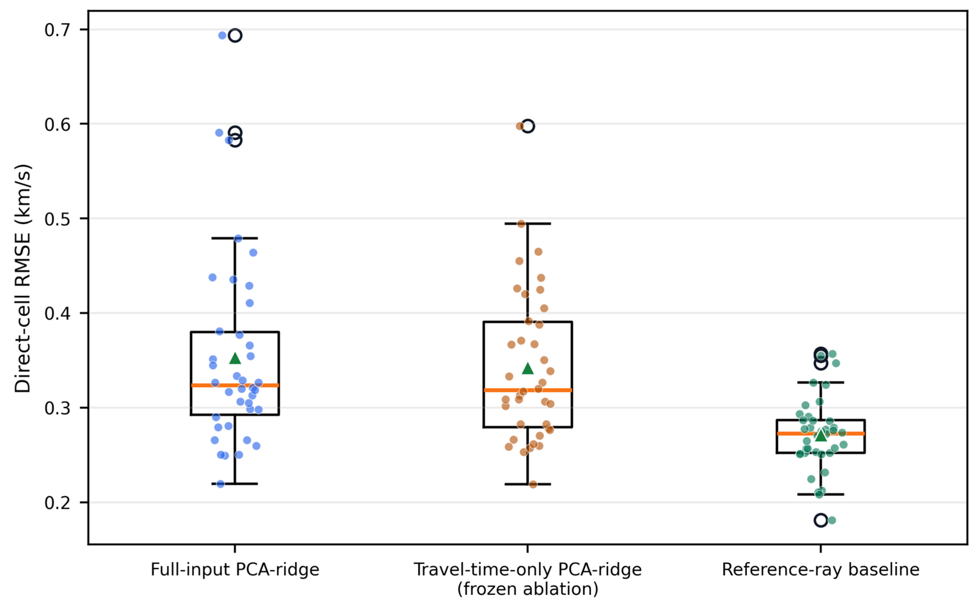
Figure 2 shows the per-target distributions behind three rows of Table 2.

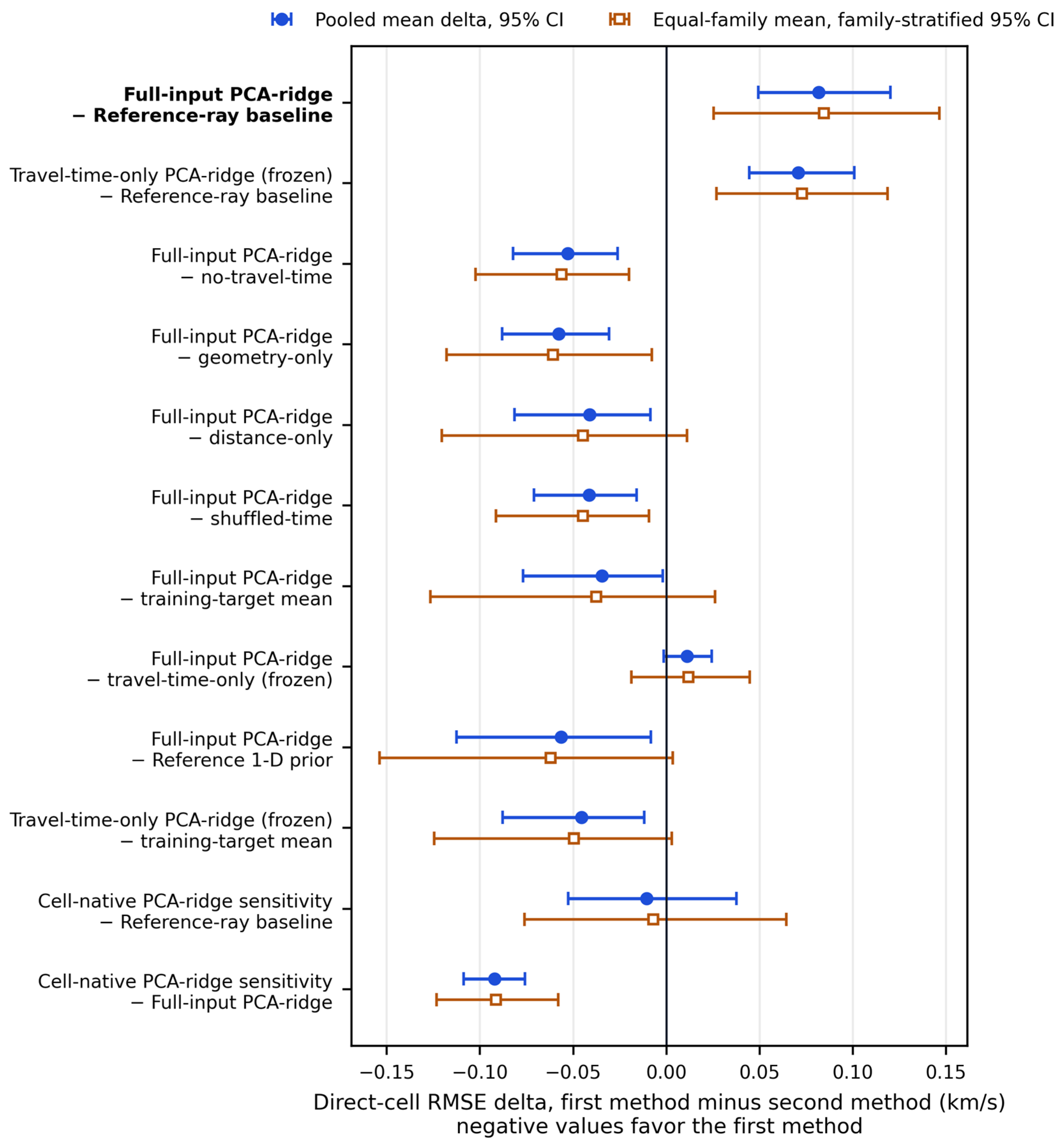
Table 3 gives the paired deltas with their pooled intervals and, beside them, the equal-family means with their family-stratified intervals, a different estimand: against the no-travel-time control, the equal-family mean is −0.0563 km/s with family-stratified CI of [−0.102, −0.0201] km/s, and against the frozen shuffled-time association control, it is −0.0448 km/s with family-stratified CI of [−0.0914, −0.00927] km/s. Both resolve in the same direction as their pooled counterparts. The shuffled control, whose construction is defined in Section 2.8, is a case-level association control, not a decomposition of uniquely geological timing information and not a causal test of geological information.

Adding source and receiver coordinates and Euclidean distance to the travel-time-only representation did not produce an improvement whose paired interval excludes zero under the frozen ablation: the paired delta is +0.0110 km/s with pooled CI of [−0.00140, +0.0244] km/s and 19 versus 19 target-level wins and losses, and the equal-family mean is +0.0119 km/s with family-stratified CI of [−0.0187, +0.0447] km/s. The independently tuned travel-time-only sensitivity selected K = 32 and α_ridge = 1000 on validation and gave test RMSE 0.343 km/s; that secondary result is not substituted for the frozen ablation. Both are specific to the selected feature representation and PCA-ridge estimator: the ablations evaluate the effect of altering the observation inputs under the frozen full-input-selected configuration rather than comparing independently optimized feature representations, and they do not establish that geometry is intrinsically uninformative.

The primary representation is order-dependent by construction: position j in the fixed-length vector denotes a source and station identifier index, not a fixed physical ray (Section 2.5). Whether the reported observation-information effect depends on that arbitrary ordering is a separate question from the shuffled-time control, which destroys the target-acquisition association rather than re-ordering an information-preserving encoding. Re-sorting each case’s 384 complete eight-field tuples by acquisition geometry, which adds and removes nothing, and then repeating the whole workflow with validation-only selection, lowers test direct analytic cell-center RMSE from 0.353 to 0.310 km/s, a paired difference of −0.0430 km/s with pooled CI of [−0.0760, −0.0149] km/s and 23 of 38 targets improved. That is a complete-workflow effect rather than an isolated ordering effect: the geometry-canonical run also reselected the ridge penalty on validation, to α_ridge = 100 rather than 1000, and no fixed-penalty control was run, so the reduction cannot be apportioned between the re-ordering and the reselection. What it does show is that the benchmark’s headline gap is materially sensitive to the observation representation and its associated validation selection, and is not a property of first-arrival information alone. The primary ordering is unchanged: geometry-canonical full-input PCA-ridge is still above the reference-ray baseline by +0.0386 km/s with pooled CI of [+0.0222, +0.0584] km/s, against +0.0816 km/s for the identifier ordering. A single fixed permutation applied identically to every case leaves the test result unchanged to five decimals, as a linear model with per-column standardization must. Table S10 of Supplementary Materials Section S20 reports both variants and their selected configurations, and the deposited ordering record holds the full validation grids.

The declared identifier ordering remains the main reported comparison even though the geometry-canonical ordering scores better. The declared encoding was fixed before any test outcome was examined; the geometry-canonical variant was run later, when the declared workflow’s test results were already known, so making the better-scoring encoding the headline would be the post hoc selection that Section 2.11 describes. The dependence is itself the finding: re-ordering the same observations moves the gap to the reference-ray baseline from +0.0816 to +0.0386 km/s, and a benchmark that did not declare its encoding could have reported either.

3.4. PCA-Ridge Reconstruction Versus the Reference-Ray Baseline

The reference-ray baseline uses the observation residual t_obs − t_FSM(s₀) and the fixed path operator G_ref. The reference 1-D prior has direct analytic cell-center RMSE 0.410 km/s, whereas the validation-selected reference-ray baseline has RMSE 0.272 km/s. Because PCA-ridge is node-native and converted to cells whereas the reference-ray baseline is cell-native, the main reported comparison sets complete reconstruction workflows against each other under a common truth domain rather than parameterization-neutral inversion algorithms. Three properties of the comparison follow, and none of them is incidental. The comparator is supplied with the exact anomaly-removed generator background of four of the five families (Section 2.9), while PCA-ridge learns its target prior from the training corpus. The comparator estimates cells directly, while PCA-ridge predicts nodes that are then converted; changing only that parameterization moves the estimator from 0.353 to 0.261 km/s and leaves the paired interval for the comparison with the baseline spanning zero (Table 3 and Section 3.6). And the comparator’s reference-model fixed-ray sensitivity operator shows high sign agreement with the finite-difference FSM diagnostic and retains the positive support of the sampled cells, but agrees poorly in magnitude; because off-path cells were not sampled, general support agreement is not assessed, as reported later in this section. The main reported comparison is therefore a designated comparison of two complete, intentionally non-equivalent workflows that differ simultaneously in prior information, native output parameterization and operator construction. It is not a parameterization-matched method comparison, it does not isolate the contribution of any one of those three factors, and it does not support a general claim about learned estimators against tomographic inversion.

A predeclared local finite-difference diagnostic is reported in Supplementary Materials Figure S2, with its pooled statistics in Table S7 of Supplementary Materials Section S17 and its per-ray values in Table S13 of Supplementary Materials Section S23. The selected entries show high retention of positive reference-ray support and high agreement in sign, and very poor agreement in magnitude. Retention is not support agreement: every evaluated cell was selected to lie on a positive reference-ray path, so the diagnostic cannot see a cell that the fixed ray treats as off-path while the finite-difference derivative does not, and it measures no false-positive support away from the ray. The sign disagreement is confined to four of the twelve rays, so the pooled fraction is an average rather than a uniform property, and the magnitude disagreement does not depend on how the relative difference is normalized: the correlation and the mean absolute error between the two sensitivities, which do not divide by either sensitivity, show it directly (Supplementary Materials Section S23). These values do not validate G_ref as an exact FSM Jacobian or validated FSM linearization, and the reference-ray result is therefore interpreted as an independent reference-model fixed-ray regularized path-operator baseline under the declared benchmark.

Figure 3 plots each row of Table 3 with both of its intervals against zero.

The reference-ray baseline has lower mean direct-cell RMSE than full-input PCA-ridge: the paired delta is +0.0816 km/s, with pooled CI of [+0.0492, +0.120] km/s. Reported alongside it, the equal-family mean is +0.0845 km/s, a different estimand, with family-stratified CI of [+0.0254, +0.146] km/s. The two intervals answer different questions, which matters because the family deltas differ markedly, as Section 3.6 shows: the pooled interval describes the mean over the configured mixture of families and lets the family composition of each resample vary, whereas the family-stratified interval holds each family’s share fixed and weights the five families equally. Both exclude zero here. This is a comparison under the declared discrete operator, not a physical superiority claim. Because the two workflows differ at once in prior, parameterization and operator, the interval shows that their combined difference is not zero, not which of the three produces it; the background substitution of Supplementary Materials Section S15 varies the prior values and the cell-native sensitivity the parameterization, while operator construction was not varied. The structure-resolved metrics that support the quantitative claims follow in Section 3.5, with representative fields in Supplementary Materials Figure S4.

To examine whether the linearity of the coefficient map limits PCA-ridge, the ridge map was replaced by the one-hidden-layer network described in Section 2.7, with everything else in the workflow unchanged and its candidate grid and selection rule fixed in advance. Validation again selected a single component, with validation node RMSE 0.243 km/s against 0.240 km/s for PCA-ridge. On the test targets, the network reached 0.352 km/s against 0.353 km/s for PCA-ridge (network minus PCA-ridge −0.00158 km/s, CI [−0.0236, +0.0174] km/s, spanning zero), and it remained above the reference-ray baseline by 0.0801 km/s (CI [+0.0554, +0.108] km/s). The pooled comparison is therefore essentially unchanged, and at this component count the linearity of the coefficient map does not account for the pooled gap. Because K = 1 was again selected, the network, like PCA-ridge, predicts only the amplitude of the same, approximately depth-only, component described in Section 3.2, so this sensitivity does not relax the representational limit discussed in Section 4.2. On layered targets, however, the network recovers part of the gap to the baseline (+0.255 to +0.147 km/s) and is worse in the other four families by 0.00424 to 0.0360 km/s; the pooled figure hides this redistribution. It is one shallow architecture and is not representative of deep or convolutional models. Supplementary Materials Section S27 gives the protocol, the validation results by component count and the family means, and Table S18 gives the paired differences.

3.5. Diagnostic Sensitivities

The coverage diagnostic uses accumulated path length from the reference operator, not true-model ray coverage. The full-input minus reference-ray baseline delta remained positive across the tested thresholds; at 10 km the mean difference was +0.0861 km/s, and Supplementary Materials Figure S5 shows the per-method target-level percentile-bootstrap intervals. The result is specific to the reference-operator illumination partition and is not evidence that those paths measure true-model illumination, resolution, or recoverability.

Generator-defined structural masks show substantially larger body than background errors for the dyke-intrusion and salt-dome families, while layered and fault-side performance varies by region; for both PCA-ridge outputs (full-input and frozen travel-time-only), the layered-mask error rises from the first layer through the fourth and remains elevated in the fifth, whereas the reference-ray baseline is lower in the deeper layered masks for this test set. Mask membership is fixed by the generating model and no predicted localization detector is used, so these are descriptive recovery errors under known masks and do not establish localization capability in unlabeled data. Because each family contains only 7–8 held-out targets, the family- and mask-specific summaries are descriptive diagnostics rather than independently powered main reported comparisons. Table S17 of Supplementary Materials Section S26 reports the complete mask-resolved metrics, and Supplementary Materials Figure S4 shows representative reconstruction fields.

Under ten matched Gaussian-noise repetitions per nonzero level, full-input PCA-ridge changed very little in mean direct-cell RMSE: degradation at 0.100 s was 0.000015 km/s with across-target standard deviation (SD) 0.000231 km/s, against 0.000005 km/s with SD 0.000259 km/s for the independently tuned travel-time-only sensitivity and 0.00455 km/s with SD 0.00101 km/s for the reference-ray baseline. Table S16 of Supplementary Materials Section S25 gives those means over matched repetitions rather than additional test-set refits. At 0.100 s the perturbation is 1.04% of the median absolute travel time, which is 9.62 s over the 14,592 observations of the 38 test targets. The median absolute geological perturbation, here the difference between the observed time and the FSM time through the shared layered profile of Section 2.9, for every test target including the layered ones, is only 0.0034 s and varies strongly by family, so it is not used as a cross-family denominator and no cross-family timing-noise sensitivity claim is made. The near-zero degradation indicates low sensitivity to the tested independent zero-mean Gaussian perturbations at these amplitudes; it does not establish robustness to systematic or correlated errors, picking errors, phase misidentification, or source-location uncertainty.

Two secondary diagnostics bound the scope of the result rather than extending it, and neither was run at the selected configuration. The learning-curve trajectory of Supplementary Materials Section S14 and Table S4 is still descending where the 175-target pool ends, and the leave-one-family-out diagnostic of Supplementary Materials Section S13 and Table S3 was selected over a candidate grid that does not contain the primary K = 1, α_ridge = 1000 configuration; neither therefore estimates optimized out-of-family performance.

The forward calculation is reproducible under the stated finite-grid configuration, but the available checks do not establish continuum accuracy. The geological signal was defined as the absolute target-versus-common-background FSM timing difference under the adopted operator. For the four structured families, that common background is the shared layered profile that also defines the reference-ray reference slowness s₀. For the layered family, no fraction of signal below 0.10 s (Supplementary Materials Section S16) is defined, because the comparison background of a layered target was its own forward field; the zero layered signal entries of the archived record (Table S6) are therefore an absence of contrast by construction, not evidence that layered targets coincide with the shared profile. Table S6 of Supplementary Materials Section S16 tabulates the signal distributions, refinement discrepancies and independent-solver cross-check by family, and they show that available finite-grid diagnostic discrepancies are not uniformly smaller than the smallest target-induced timing signals. The two scales come closest in the block-anomaly family, where the independent-solver discrepancy reaches 0.0979 s against that family’s own 95th-percentile absolute geological signal of 0.134 s; in the other three structured families the 95th-percentile signal is several times the corresponding discrepancy. The refinement audit over the full predeclared list of eight geometries per family, reported in Supplementary Materials Section S24, gives a median absolute change of 0.0396 s and a maximum of 0.253 s, and of the sixteen pairs whose geological signal exceeds the 0.01 s floor, five of the sixteen have a refinement discrepancy larger than the signal itself. Supplementary Materials Tables S14 and S15 give the discrepancy by geometry and by family. The finite-grid discrepancy is therefore not merely comparable with the geological signal for some geometries; it exceeds it for an appreciable fraction of the audited ones. The independent-solver cross-check remains a fifteen-pair audit of scale, and neither audit samples the production acquisition, so neither estimates a survey-wide frequency. Because the refinement audit was enlarged and the independent-solver audit was not, the geometry dependence that enlargement exposed is untested for the solver comparison. This evidence supports a discrete-operator interpretation: the results are conditional on a reproducible finite-grid operator, with physical interpretation limited accordingly. Section 4.4 discusses what this means for the method comparison as a whole.

3.6. Family and Prior Dependence

The shared layered profile that defines the reference-ray reference slowness is the anomaly-removed generator background of the block-anomaly, dyke-intrusion, faulted and salt-dome families, but not of the layered family, whose layer velocities are sampled independently. Resolving the main reported comparison by family therefore separates targets for which the comparator holds the exact generator background from those for which it does not. The background is exact on the forward grid; at the direct cell-center endpoint its cell representation carries the interface error described in Section 2.9, common to all four background-matched families. Supplementary Materials Table S1 reports the family-resolved all-cell means and paired deltas.

The reference-ray advantage over full-input PCA-ridge is not concentrated in the families whose background the comparator holds exactly. Averaged over the four families with the exact shared background, the full-input minus reference-ray paired delta is +0.0418 km/s; for the layered family, where the comparator does not hold the exact background, it is +0.255 km/s. The same asymmetry is stronger for the cell-native sensitivity. Averaged over the four background-matched families, its paired delta against the reference-ray baseline is −0.0667 km/s, and it is higher on the layered family (+0.232 km/s). That average is not a uniform direction: three of the four family means are negative (block anomaly −0.109, dyke intrusion −0.0662, salt dome −0.0933 km/s), while the faulted-family mean is +0.00146 km/s, close to zero, with its targets split four of eight. The pooled cell-native versus reference-ray comparison reported in Table 3, whose interval spans zero, therefore averages three negative family means and one near-zero among the background-matched families against an opposing direction on the layered family.

For the cell-native sensitivity, the per-target sign counts of Supplementary Materials Table S1 show the same asymmetry without averaging (all seven layered targets favor the baseline, against seven of 31 in the other four families); for full-input PCA-ridge they do not, since the faulted family favors the baseline on all eight targets. The mask-averaged deltas of Supplementary Materials Section S11 localize the comparator’s advantage within the four structured families. The comparator’s measured advantage is largest in the layered family, whose background it does not hold, and smallest, or absent, in the families whose generator background it holds. The pooled counts are the wins/losses/ties column of Table 3, where the baseline is closer to truth on 31 of 38 targets than the full-input workflow and on 14 of 38 than the cell-native sensitivity.

These family- and mask-resolved summaries are descriptive diagnostics for the reason given in Section 3.5, and Section 4.2 discusses the readings consistent with them. Supplementary Materials Section S15 and Table S5 report the background-substitution comparator sensitivity, which replaces the comparator’s exact background values with training-derived estimates: the exact values lower the comparator’s RMSE by a small but nonzero 0.00216 km/s (training-derived minus exact, CI [+0.00022, +0.00387] km/s), under 3% of the main reported difference, and the main reported comparison is essentially unchanged without them.

4. Discussion

4.1. Observation Information and the Target Prior

The shuffled-time comparison of Section 3.3 is a case-level association effect, not evidence that one estimator is better, for the reasons given in Section 2.8. The difference between full-input PCA-ridge and the training-target mean is negative in this test set, has a family-stratified interval that spans zero, and remains a secondary comparison (Table 3). The training-target mean is a substantive prior-only comparator, and all these comparisons are conditional on this estimator, fixed-length representation, target-and-acquisition distribution, and finite-grid operator.

4.2. PCA-Ridge, the Target Prior, and the Reference-Ray Baseline

The near-tie between full-input PCA-ridge and the frozen travel-time-only ablation is specific to the present fixed-length representation and selected linear coefficient map: the independently tuned travel-time-only sensitivity reaches a similar test RMSE under a very different component count. Neither result is known to hold for other encodings or nonlinear maps; the network of Section 3.4 was fitted to the full-input features only, so it does not test the travel-time-only result.

Changing only the target parameterization materially affects the apparent workflow ranking (Section 3.4), and the near-zero pooled difference under the cell-native basis averages opposing family-level directions (Section 3.6) rather than describing a uniform absence of difference. Two readings are consistent with the family-resolved diagnostics and the present design does not separate them. The first is representational: a single retained principal component fitted across five heterogeneous families is, as Section 3.2 shows for the node-native basis, close to a depth-only profile, which provides limited capacity for localized bodies; although the layered family also varies only with depth, its layer boundaries and five layer velocities vary independently between targets, which one fixed depth profile scaled by a single coefficient cannot span. The second is that the comparator may retain a structural prior advantage on layered targets that is distinct from an exact-background advantage, because a one-dimensional layered reference model matches the structural form of a layered target even when its velocities differ. Both readings rest on family means over seven or eight targets and on the per-family counts of targets favoring each method in Supplementary Materials Table S1, not on per-family intervals, and are offered as interpretations rather than established family effects. Both are prior-related, and the background-substitution sensitivity of Supplementary Materials Section S15 indicates that the exact shared background values alone do not account for them. The neural-network sensitivity of Section 3.4 narrows the layered gap with the same single component, at a cost in the other four families, so the linear coefficient map may account for part of that gap.

On the common direct-cell endpoint the reference-ray baseline has the lower RMSE (Section 3.4). That is comparative evidence under the declared discrete operator, not evidence that the selected learning method is inferior to tomography in general, and the three differences between the workflows do not have equal evidential standing: target parameterization (under the cell-native basis the point estimate reverses sign, although its paired interval spans zero; Table 3) and background values (whose measured contribution is small under frozen regularization; Supplementary Materials Section S15) were varied experimentally, whereas operator construction was not varied and therefore remains an unresolved source of non-equivalence rather than a demonstrated sensitivity of the ordering. The dependence of the ranking on the representation choices is the benchmark result; the ordering itself is not a method ranking. The comparator remains a transparent baseline with a different inductive bias rather than a full nonlinear tomography workflow, since it uses fixed reference geometry and does not update paths after recovery. In addition, the eight-corner transform contributes direct-cell error near sharp analytic interfaces in both workflows: PCA-ridge applies it to its node predictions, and the baseline’s prior carries it through the reference profile, as Section 2.9 describes.

4.3. Structure and Operator Dependence

The mask-resolved errors of Section 3.5 show that a global error does not describe recovery uniformly. Dyke and salt-dome body errors remain large even where the structures span several target cells, which is consistent with combined limitations from illumination, target representation, and observation-to-model ambiguity; these are descriptive synthetic mask results, not localization evidence for unlabeled data. Reference-operator coverage provides a useful secondary partition, but, consistent with the role of sensitivity tests in tomography [32], that partition is generated by the baseline and is not true-model resolution. Because many target-induced timing signals are small relative to the available finite-grid diagnostics (Section 3.5), structure rankings and physical interpretation must be read together with the operator and metric specification. The LOFO diagnostic is an exploratory assessment of family-extrapolation behavior under its stored node/eight-corner metrics; it is not a primary direct-cell endpoint and does not measure transfer to natural geology.

4.4. Scope and External Validity

This is a discrete-operator benchmark: a reproducible evaluation of reconstruction methods under a declared operator, prior, acquisition and uncertainty procedure. It is not a validated continuum approximation for all configured structures, a field-scale forward-model study, or a real-data tomography result. The benchmark compares the frozen validation-selected workflows defined by their prespecified candidate grids rather than attempting exhaustive hyperparameter optimization.

The corpus contains five simplified synthetic families, one acquisition realization per target, exact synthetic source and receiver coordinates, and a 2.5 km target grid. The uniform independently sampled acquisition is a controlled synthetic design rather than a model of the spatial distribution of earthquakes and stations in a specific field setting. As Section 2.3 states, that one-to-one pairing makes this an evaluation over the joint target-and-acquisition distribution, within which target and acquisition effects cannot be decomposed. The tested timing perturbations are independent zero-mean Gaussian noise, the LOFO diagnostic measures extrapolation among the configured families under its stored node/eight-corner metrics, and the learning curve remains a stored node/eight-corner training-pool sensitivity through 175 targets. These analyses expose bounded failure modes but do not measure natural-geology transfer, source uncertainty, correlated picking errors, or deployment robustness.

Two further limitations follow from the declared encoding and from the sparseness of the forward audits. The primary fixed-length PCA-ridge encoding is order-dependent: position j in the observation vector denotes a source and station identifier index within a case, not a geometrically invariant ray identity, and because acquisition geometry is resampled independently for every target that position carries no stable physical meaning across samples. The shuffled-time control destroys the target-acquisition association rather than re-ordering an information-preserving encoding, so it does not test this. The geometry-canonical sensitivity of Section 3.3 and Supplementary Materials Section S20 addresses it, though not in isolation: the complete geometry-canonical workflow, which re-orders the same observations and includes a validation reselection of the ridge penalty in the same step, lowers test RMSE by 0.0430 km/s, roughly half the main reported gap; no fixed-penalty control separates the two contributions. Observation-content conclusions are therefore properties of the declared identifier-ordered encoding rather than of first-arrival information independently of encoding, and the magnitude of that dependence is measured. The forward diagnostics are the second limitation: as Section 3.5 reports, neither samples the production acquisition.

The forward discrepancy bears on the whole quantitative comparison, not only on the forward diagnostics. Errors are measured against the analytic velocity field, so the finite-grid discrepancy does not contaminate the reference against which every workflow is scored. It enters through the observations instead. The travel times are those of the discrete operator, and on some audited geometries halving the grid spacing from 2.5 km to the adopted 1.25 km changes them by more than the geological signal, so the benchmark measures what can be recovered from these discrete observations, not from continuum travel times. The two workflows also relate to that operator differently: PCA-ridge learns directly from its outputs, whereas the reference-ray baseline approximates its sensitivities with fixed rays, whose agreement with finite differences in an auxiliary FSM on the target-cell grid, not the label operator itself, is assessed in Section 3.4 and Supplementary Materials Tables S7 and S13. Part of the paired difference may therefore reflect this operator mismatch rather than a difference in the ability to recover structure.

5. Conclusions

On this benchmark, the size of the apparent gap between workflows depends on how observations are encoded and how targets are parameterized, not only on the estimator; under the cell-native parameterization the pooled difference is not resolved, and its sign varies by family. We showed this on a target-atomic synthetic benchmark of 250 unique geological targets from five parameterized families, each with one recorded acquisition realization and 384 finite travel-time observations, split 175/37/38 with no exact target-hash overlap, with geological targets rather than source–receiver observations as the independent unit for uncertainty.

Each value listed below is the mean per-target direct analytic cell-center RMSE over the 38 held-out test targets, for a configuration selected on the 37 validation targets only:

• The declared full-input PCA-ridge workflow, node-native and converted to cells by eight-corner averaging, with identifier-ordered observations, K = 1 and α_ridge = 1000: 0.353 km/s;
• The same declared workflow with a small neural network in place of the ridge coefficient map, a secondary sensitivity that again selected K = 1, with one hidden layer of 16 neurons and weight penalty 10: 0.352 km/s;
• The complete geometry-canonical workflow, which re-orders the identical observations by acquisition geometry and reselects on validation, giving K = 1 and α_ridge = 100: 0.310 km/s;
• PCA-ridge with a cell-native target parameterization and the same observations, with K = 1 and α_ridge = 1000: 0.261 km/s;
• The reference-ray baseline, a fixed-ray regularized inversion from the configured layered reference model, which is the exact background of four of the five families, with damping 0.001 and smoothing 10.0: 0.272 km/s.

The comparator leads the main reported comparison by +0.0816 km/s and still leads after the re-ordering by +0.0386 km/s, both with intervals excluding zero, while the cell-native interval spans zero and averages opposing family-level directions (Section 3.6). The selected node-native estimator uses source and receiver coordinates, Euclidean distance, and travel time, with K = 1 and α_ridge = 1000 chosen on validation; the interval against the frozen travel-time-only ablation spans zero, and the no-travel-time, geometry-only and distance-only controls are zero-target-information behavioral controls under the independent acquisition/geology seed design. The main reported comparison is conditional on the declared discrete operator and establishes no universal superiority of a path-based or learning-based method.

The contribution is a transparent discrete-operator benchmark that makes the observation operator, target prior, estimator, baselines, metric domain, and target-level uncertainty explicit. Its limitations define the scope of inference:

• The study is synthetic only, with five simplified families, and makes no claim about field data;
• The two compared workflows differ at once in prior, target parameterization and operator construction, so the paired difference is not attributed to any one of them;
• The declared encoding orders features by an arbitrary per-case identifier, and re-ordering them by geometry, with validation reselection of the penalty, lowers the PCA-ridge error materially;
• All travel times come from one finite-grid solver configuration; of the 40 audited source–receiver pairs, 16 have a geological signal above the 0.01 s floor, and for five of these the refinement discrepancy exceeds the signal;
• Each target has a single acquisition realization, so target and acquisition effects cannot be separated;
• Test targets come from the same generator as training targets, and close analogs were retained, so test scores are in-distribution scores, not measures of performance on new geology;
• The corpus is small for a learned estimator: with 175 training targets the learning curve, run at a configuration other than the selected one, is still descending, and the selected K = 1 is specific to this corpus;
• The tested noise is independent zero-mean Gaussian timing noise only, and the extrapolation diagnostics are secondary;
• The main reported comparison was designated after the configurations were frozen, and its intervals describe test-set sampling variation rather than significance.

Within these limits, the benchmark supports reproducible comparative evaluation, not continuum-exact forward validation, field-scale accuracy, or real-world geological transfer.

Several directions for future research follow from these limitations. The most direct are field or field-like observations; repeated acquisitions per target, which would separate target and acquisition effects; travel times from a second forward solver or a refined grid, which would bound the solver dependence; deep learned estimators and encodings that do not depend on the order of the observations; and a path-updating tomographic comparator. Except for field observations, which have no known true velocity and would need a different evaluation, each can be added under the same declared evaluation, so that its effect on the apparent ordering is measured rather than assumed.

References

1. Nolet, G. (Ed.) Seismic Tomography: With Applications in Global Seismology and Exploration Geophysics; D. Reidel: Dordrecht, The Netherlands, 1987. [Google Scholar] [CrossRef] [Scilit]
2. Aki, K.; Lee, W.H.K. Determination of three-dimensional velocity anomalies under a seismic array using first P arrival times from local earthquakes: 1. A homogeneous initial model. J. Geophys. Res. 1976, 81, 4381–4399. [Google Scholar] [CrossRef] [Scilit]
3. Thurber, C.H. Earthquake locations and three-dimensional crustal structure in the Coyote Lake area, central California. J. Geophys. Res. Solid Earth 1983, 88, 8226–8236. [Google Scholar] [CrossRef] [Scilit]
4. Rawlinson, N.; Fichtner, A.; Sambridge, M.; Young, M.K. Seismic tomography and the assessment of uncertainty. Adv. Geophys. 2014, 55, 1–76. [Google Scholar] [CrossRef] [Scilit]
5. Thurber, C.H.; Kissling, E. Advances in travel-time calculations for three-dimensional structures. In Advances in Seismic Event Location; Thurber, C.H., Rabinowitz, N., Eds.; Modern Approaches in Geophysics; Springer: Dordrecht, The Netherlands, 2000; Volume 18, pp. 71–99. [Google Scholar] [CrossRef] [Scilit]
6. Giroux, B. ttcrpy: A Python package for traveltime computation and raytracing. SoftwareX 2021, 16, 100834. [Google Scholar] [CrossRef] [Scilit]
7. Zhao, H. A fast sweeping method for eikonal equations. Math. Comput. 2005, 74, 603–627. [Google Scholar] [CrossRef] [Scilit]
8. Um, J.; Thurber, C.H. A fast algorithm for two-point seismic ray tracing. Bull. Seismol. Soc. Am. 1987, 77, 972–986. [Google Scholar] [CrossRef] [Scilit]
9. Koketsu, K.; Sekine, S. Pseudo-bending method for three-dimensional seismic ray tracing in a spherical earth with discontinuities. Geophys. J. Int. 1998, 132, 339–346. [Google Scholar] [CrossRef] [Scilit]
10. Haslinger, F.; Kissling, E. Investigating effects of 3-D ray tracing methods in local earthquake tomography. Phys. Earth Planet. Inter. 2001, 123, 103–114. [Google Scholar] [CrossRef] [Scilit]
11. Earp, S.; Curtis, A. Probabilistic neural network-based 2D travel-time tomography. Neural Comput. Appl. 2020, 32, 17077–17095. [Google Scholar] [CrossRef] [Scilit]
12. Yildirim, I.E.; Alkhalifah, T.; Yildirim, E.U. Machine learning-enabled traveltime inversion based on the horizontal source-location perturbation. Geophysics 2022, 87, U1–U8. [Google Scholar] [CrossRef] [Scilit]
13. Jo, J.H.; Ha, W. Seismic traveltime tomography using deep learning. IEEE Trans. Geosci. Remote Sens. 2023, 61, 5923111. [Google Scholar] [CrossRef] [Scilit]
14. Jo, J.H.; Ha, W. Seismic traveltime tomography using transfer learning. IEEE Trans. Geosci. Remote Sens. 2024, 62, 5931214. [Google Scholar] [CrossRef] [Scilit]
15. Song, C.; Geng, H.; Wang, Y.; Waheed, U.B.; Liu, C. Simultaneous P- and S-wave seismic traveltime tomography using physics-informed neural networks. Geophys. Prospect. 2025, 73, e70034. [Google Scholar] [CrossRef] [Scilit]
16. Yang, S.; Zhang, H.; Gao, L.; Chen, Z.; Qian, J.; Yang, H. Seismic traveltime tomography with deep neural network reparameterization: The method and its application to Central Chile. J. Geophys. Res. Solid Earth 2026, 131, e2026JB034630. [Google Scholar] [CrossRef] [Scilit]
17. Wang, Y.; Jia, Z.; Jiang, B.; Lu, W. Space correlation constrained physics informed neural network for seismic tomography. J. Geophys. Res. Mach. Learn. Comput. 2026, 3, e2025JH000855. [Google Scholar] [CrossRef] [Scilit]
18. Zeng, Y.; Bai, M.; Chen, Y. EKtomo: A physics-informed neural network approach for robust crosswell travel-time tomography. Geophys. Prospect. 2026, 74, e70184. [Google Scholar] [CrossRef] [Scilit]
19. Zelt, C.A.; Haines, S.; Powers, M.H.; Sheehan, J.; Rohdewald, S.; Link, C.; Hayashi, K.; Zhao, D.; Zhou, H.-W.; Burton, B.L.; et al. Blind test of methods for obtaining 2-D near-surface seismic velocity models from first-arrival traveltimes. J. Environ. Eng. Geophys. 2013, 18, 183–194. [Google Scholar] [CrossRef] [Scilit]
20. Deng, C.; Feng, S.; Wang, H.; Zhang, X.; Jin, P.; Feng, Y.; Zeng, Q.; Chen, Y.; Lin, Y. OpenFWI: Large-scale multi-structural benchmark datasets for full waveform inversion. Adv. Neural Inf. Process. Syst. 2022, 35, 6007–6020. [Google Scholar] [CrossRef] [Scilit]
21. AlAli, A.; Anifowose, F. Seismic velocity modeling in the digital transformation era: A review of the role of machine learning. J. Pet. Explor. Prod. Technol. 2022, 12, 21–34. [Google Scholar] [CrossRef] [Scilit]
22. Wu, Y.; Lin, Y. InversionNet: An efficient and accurate data-driven full waveform inversion. IEEE Trans. Comput. Imaging 2020, 6, 419–433. [Google Scholar] [CrossRef]
23. Dramsch, J.S. 70 years of machine learning in geoscience in review. Adv. Geophys. 2020, 61, 1–55. [Google Scholar] [CrossRef] [Scilit]
24. Bianco, M.J.; Gerstoft, P. Travel time tomography with adaptive dictionaries. IEEE Trans. Comput. Imaging 2018, 4, 499–511. [Google Scholar] [CrossRef] [Scilit]
25. Guo, R.; Li, M.; Yang, F.; Xu, S.; Abubakar, A. First arrival traveltime tomography using supervised descent learning technique. Inverse Probl. 2019, 35, 105008. [Google Scholar] [CrossRef] [Scilit]
26. Yang, H.; Li, P.; Ma, F.; Zhang, J. Building near-surface velocity models by integrating the first-arrival traveltime tomography and supervised deep learning. Geophys. J. Int. 2023, 235, 326–341. [Google Scholar] [CrossRef] [Scilit]
27. Wang, F.; Yang, B.; Wang, R.; Qiu, H. Seismic traveltime tomography with label-free learning. IEEE Trans. Geosci. Remote Sens. 2024, 62, 5911515. [Google Scholar] [CrossRef] [Scilit]
28. Wilkinson, M.D.; Dumontier, M.; Aalbersberg, I.J.; Appleton, G.; Axton, M.; Baak, A.; Blomberg, N.; Boiten, J.-W.; da Silva Santos, L.B.; Bourne, P.E.; et al. The FAIR Guiding Principles for scientific data management and stewardship. Sci. Data 2016, 3, 160018. [Google Scholar] [CrossRef] [Scilit] [PubMed]
29. Jolliffe, I.T.; Cadima, J. Principal component analysis: A review and recent developments. Philos. Trans. R. Soc. A 2016, 374, 20150202. [Google Scholar] [CrossRef] [Scilit] [PubMed]
30. Hoerl, A.E.; Kennard, R.W. Ridge regression: Biased estimation for nonorthogonal problems. Technometrics 1970, 12, 55–67. [Google Scholar] [CrossRef]
31. White, M.C.A.; Fang, H.; Nakata, N.; Ben-Zion, Y. PyKonal: A Python package for solving the eikonal equation in spherical and Cartesian coordinates using the fast marching method. Seismol. Res. Lett. 2020, 91, 2378–2389. [Google Scholar] [CrossRef] [Scilit]
32. Rawlinson, N.; Spakman, W. On the use of sensitivity tests in seismic tomography. Geophys. J. Int. 2016, 205, 1221–1243. [Google Scholar] [CrossRef] [Scilit]
Figure 1. Branched benchmark workflow. The common synthetic target and case record (saved acquisition geometry together with generated travel times) feed separate full-input principal component analysis ridge (PCA-ridge) and reference-ray baseline branches; both meet only at the common direct analytic cell-center evaluation endpoint. The true-model ray path is retained only as diagnostic information and is not a feature of the declared full-input PCA-ridge representation.
Applsci 16 09941 g001
Figure 2. Per-target direct cell-center RMSE distributions for full-input PCA-ridge, the frozen travel-time-only ablation, and the reference-ray baseline on the 38 held-out test targets. Each method shows all 38 target-level values as deterministic jittered points; green triangles denote means and thick lines denote medians; boxes span the interquartile range, whiskers reach the most extreme values within 1.5 interquartile ranges of the box, and hollow circles mark values beyond.
Applsci 16 09941 g002
Figure 3. Paired target-level comparisons of Table 3. For each comparison, the filled circle and its bar are the pooled mean RMSE delta and its paired percentile-bootstrap 95% CI over the 38 test targets; the open square and its bar are the equal-family mean and its family-stratified 95% CI, a different estimand. Each delta is first method minus second method, so negative values favor the first method; the vertical line marks zero. The bold label is the main reported comparison; the other rows are secondary or diagnostic, and no row is a hypothesis test.
Applsci 16 09941 g003