Integrating Simulated Clinical Outcomes and Nonlinear HRV Metrics in Fibromyalgia Rehabilitation: A Dual-Layer Metric- and Signal-Level Simulation Framework

Abstract

Nonlinear heart rate variability (HRV) metrics may complement scales, but metric-level simulation alone cannot test algorithm implementation or stability under signal imperfections. We evaluated a dual-layer simulation framework for fibromyalgia rehabilitation research. Layer A used a synthetic dataset (n = 48; seed 20,260,724) and 1000 Monte Carlo replicates in five scenarios. Layer B verified Higuchi fractal dimension (HFD), detrended fluctuation analysis (DFA α), and a finite-time divergence index on canonical signals and 120 synthetic 10 min RR interval tachograms analyzed at 2, 5, and 10 min, with 1% and 5% artifact burdens and varied settings. Under the null scenario, family-wise rejection rates were 3.6% for longitudinal tests and 5.5% for correlations; a latent common cause scenario produced correlation rejections in 95.9% of replicates. Canonical checks yielded HFD values of 1.029 for a sinusoid and 1.999 for white noise, while logistic-map divergence was 0.694, close to ln(2) = 0.693. In tachograms, HFD varied mainly with kmax, DFA with artifacts and scale range, and divergence with duration and embedding; no divergence fit met the R² ≥ 0.90 criterion. The framework separates statistical performance from signal processing validity but provides no evidence of treatment efficacy, autonomic recovery, or biomarker validity.

1. Introduction

Fibromyalgia is a chronic and heterogeneous syndrome characterized by widespread pain, fatigue, sleep disturbance, cognitive complaints, and reduced functional capacity. Its estimated prevalence in the general population is approximately 2–4%, with a higher prevalence among women, and its clinical burden is amplified by frequent comorbidities such as anxiety, depression, sleep disorders, and reduced participation in everyday activities [1,2]. Despite substantial advances, diagnosis and monitoring remain difficult because symptoms fluctuate over time and are influenced by biological, psychological, and environmental factors [3].

Current pathophysiological models emphasize central sensitization, altered descending pain modulation, neuroendocrine and autonomic dysfunction, and neuroimmune interactions [4,5,6,7,8]. Autonomic imbalance and reduced parasympathetic modulation have repeatedly been reported in chronic pain and fibromyalgia, supporting HRV as a noninvasive measure of cardiac autonomic regulation [9,10,11,12].

Clinical outcomes can be summarized with the Visual Analog Scale (VAS), the Fibromyalgia Impact Questionnaire (FIQ) [13], and health-related quality-of-life instruments such as the 12-item Short Form Health Survey (SF-12) [14]. Conventional time- and frequency-domain HRV indices add physiological information but are sensitive to recording length, respiratory pattern, stationarity, and preprocessing [15,16]. They summarize variability within predefined domains and do not directly characterize scale-dependent irregularity, long-range correlation structure, or local trajectory divergence.

Complex systems theory provides a complementary framework for rehabilitation research. Biological signals often exhibit irregular but structured fluctuations across temporal scales. In adaptive systems, variability is neither purely random nor rigid; it can reflect the capacity to respond to internal and external perturbations [17,18,19]. Loss of complexity, excessive regularity, or unstructured variability may indicate reduced adaptability or impaired regulation depending on the physiological context.

HFD, DFA α, and finite-time divergence characterize different signal properties. HFD quantifies scale-dependent geometric irregularity [20]; DFA α estimates the scaling of detrended fluctuations over a specified range of windows [21,22]; and finite-time divergence summarizes local trajectory separation under fixed reconstruction settings [23,24]. None of these established metrics, or the standard statistical tests used below, is novel by itself. The methodological question is whether a transparent workflow behaves as intended at both the statistical and signal processing levels under null, attenuated, dissociated, confounded, shortened, and artifact-contaminated conditions.

Changes in nonlinear metrics do not have a universally beneficial direction. Higher HFD or DFA α may reflect structured variability in one context and noise, nonstationarity, or preprocessing artifacts in another. Their meaning depends on disease state, acquisition conditions, respiratory behavior, medication, segment length, and analysis settings. Accordingly, this study treats all nonlinear metrics as simulated analytical variables and does not equate increased complexity with recovery.

The primary aim was to specify and stress test, entirely through computer simulation, a reproducible framework for the joint analysis and reporting of simulated clinical-scale variables and nonlinear HRV metrics within a modeled fibromyalgia rehabilitation pathway. The objectives were to (i) disclose the complete metric-level data-generating mechanism; (ii) separate a single worked example from repeated Monte Carlo simulation; (iii) quantify effect estimate stability, confidence interval coverage, and multiplicity-adjusted rejection rates; (iv) verify the numerical implementation of HFD, DFA α, and finite-time divergence on canonical synthetic signals; and (v) quantify the sensitivity of these metrics to RR recording duration, artifacts, preprocessing, and analysis settings. No actual participants, interventions, or physiological recordings were analyzed.

2. Materials and Methods

2.1. Study Design, Aim, and Scope of Inference

The study comprises two explicitly separated simulation layers. Layer A retains the metric-level framework, in which derived clinical and nonlinear variables are generated directly to evaluate statistical operating characteristics. Layer B is an independent signal-level verification and robustness study in which HFD, DFA α, and finite-time divergence are computed from canonical synthetic signals and synthetic RR interval tachograms. Layer B evaluates implementation behavior and sensitivity to recording length, artifacts, preprocessing, and parameter settings; it does not establish physiological or clinical validity.

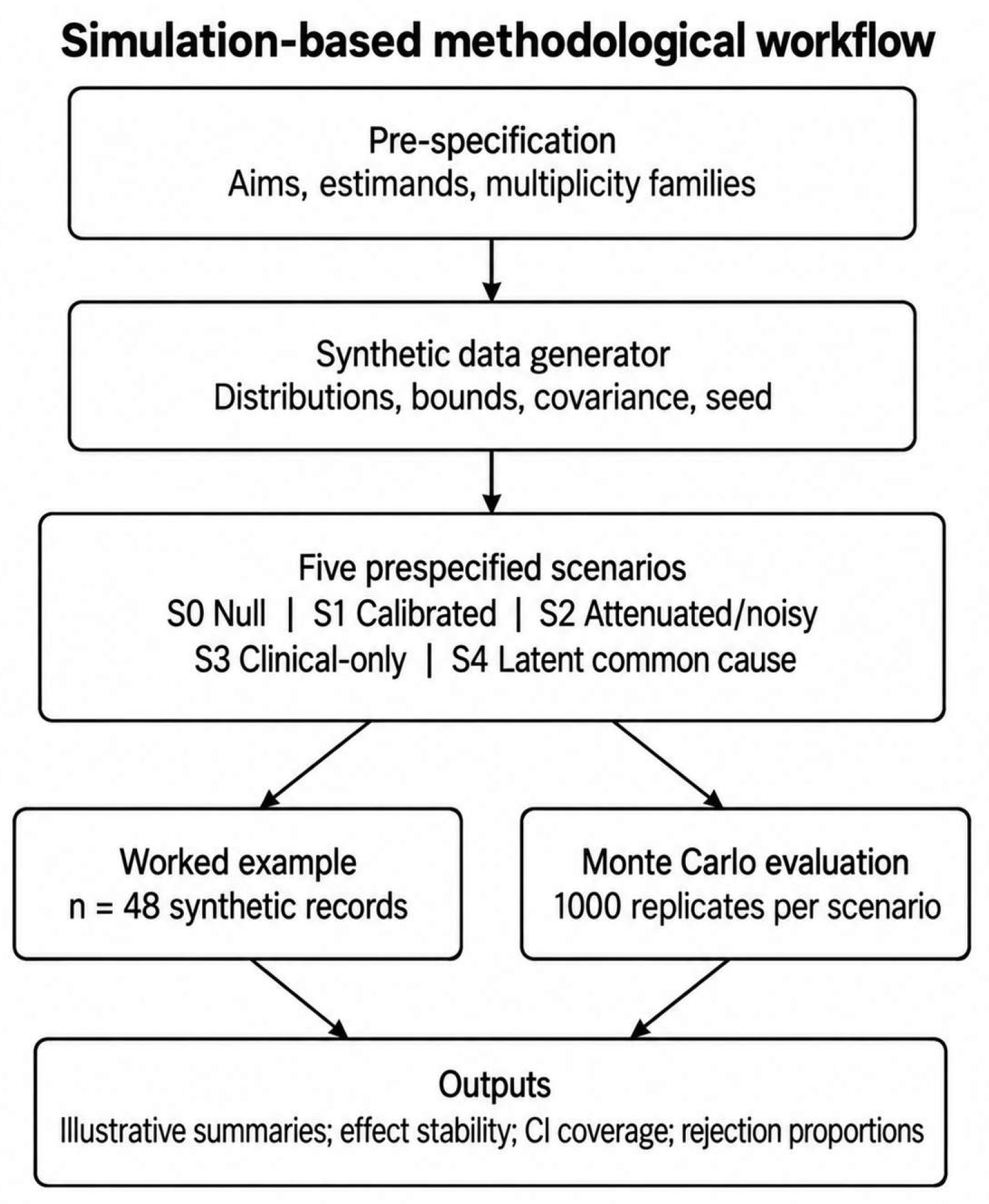
This methodological simulation study contains only computer-generated analytical units. A worked dataset of 48 synthetic records demonstrates the proposed tables and figures, whereas statistical operating characteristics were evaluated across 1000 independent replicates in each scenario.

Layer A integrates six simulated longitudinal variables—three clinical-scale variables and three nonlinear HRV-related variables—within separate testing families and includes negative-control scenarios that expose circularity and confounding. Layer B independently tests the nonlinear algorithms on generated signals. The study does not propose a new HFD, DFA, or divergence algorithm, a clinical prediction model, or provide evidence that rehabilitation changes autonomic physiology.

The size of the worked synthetic dataset (n = 48) was chosen solely to preserve the scale of the original methodological example. This number does not represent a recruited clinical sample and was not derived from a clinical sample-size calculation. It is sufficient for illustrating repeated-measures and correlation procedures but is not presented as a sufficient basis for multivariable prediction or clinical validation.

2.1.1. ADEMP Simulation Specification

The simulation was planned using the ADEMP structure: aims, data-generating mechanisms, estimands, methods, and performance measures [25]. The estimands were mean improvement-oriented changes for six outcomes and nine cross-domain Pearson correlations between three clinical and three nonlinear change scores. Performance measures were median effect estimates, 2.5th–97.5th empirical percentiles, 95% confidence interval coverage, Holm-adjusted rejection proportions, and Monte Carlo standard errors. Scenario definitions and analysis settings were fixed in the code before simulation; the study was not preregistered.

2.1.2. Independent Simulation Scenarios

Five scenarios were specified before analysis (

Table 1. Prespecified simulation scenarios.

Scenario	Mean Structure	Dependence Structure/Purpose
S0 Null	No T1/T2 mean changes	No shared change factor; strict null
S1 Calibrated	Full target shifts	Shared change factor, loading 0.75; workflow check
S2 Attenuated/noisy	50% shifts; SD × 1.25	Shared change factor, loading 0.40; weaker signal
S3 Clinical-only	Clinical shifts only	Separate clinical/HRV factors; cross-domain dissociation
S4 Latent common cause	No mean changes	Shared factor, loading 0.75; unmeasured common cause stress test

). S0 was a strict null for mean changes and cross-domain change correlations. S1 reproduced the full target mean shifts and a shared longitudinal factor. S2 halved the mean shifts, inflated standard deviations by 25%, and reduced shared coupling. S3 retained clinical changes but set nonlinear means unchanged and used separate clinical and HRV change factors. S4 had no mean changes but included a shared latent factor, representing an unmeasured common cause such as respiration, arousal, or activity.

S1 deliberately embeds the expected trajectory and therefore cannot validate it; the recovery of S1 targets is a code and workflow check. The other scenarios evaluate distinct failure modes: S0 assesses false-positive control, S2 weakens the embedded signal, S3 separates clinical and nonlinear changes, and S4 introduces a shared latent cause without mean change. Five scenarios were specified before analysis (Table 1).

2.2. Modeled Clinical Assessment Framework

For contextual purposes only, the synthetic data-generating model was structured around a hypothetical 8-week, 24-session multidisciplinary rehabilitation pathway. T0, T1, and T2 represent simulated assessment time points corresponding conceptually to baseline, program midpoint, and post-program evaluation, respectively. They do not represent actual patient visits or measurements. No patients were recruited, no rehabilitation intervention was delivered, and no attendance data, treatment responses, adverse events, or dropouts were recorded.

The simulated clinical variables were VAS (0–10), FIQ (0–100), and SF-12 (0–100). The nonlinear variables were HFD (bounded between 1 and 2), DFA α (bounded between 0.2 and 1.5), and a finite-time divergence index (bounded between 0 and 0.5). These prespecified numerical limits constrained the generator; they are neither normative ranges nor diagnostic or clinically meaningful thresholds. The metric-level values were generated directly and were not calculated from physiological recordings.

Protocol Characteristics Excluded from Inference

The data generator did not simulate recruitment, consent, session attendance, medication changes, adverse events, rejected recordings, or device logs. These items were removed from the Results because reporting them as observations would incorrectly imply a real clinical cohort. Future validation studies should prespecify and report them as actual process measures.

The latent common cause scenario is not a correlation null; its purpose is to show that a high marginal correlation detection rate can arise without a direct clinical-to-HRV mechanism.

2.3. Synthetic Data Generation

Metric-level values were drawn from a bounded 18-variable multivariate Gaussian model (six variables × three time points). The target mean and standard deviation for each variable are listed in

Table 2. Distributional targets used for the calibrated synthetic data generator (mean ± standard deviation).

Metric	T0	T1	T2
VAS	7.60 ± 1.20	5.10 ± 1.07	3.79 ± 1.07
FIQ	68.40 ± 9.70	54.20 ± 8.88	41.70 ± 8.67
SF-12	34.20 ± 6.50	41.79 ± 5.76	48.60 ± 5.99
HFD	1.36 ± 0.08	1.48 ± 0.07	1.57 ± 0.06
DFA α	0.64 ± 0.09	0.76 ± 0.08	0.86 ± 0.07
Finite-time divergence	0.21 ± 0.05	0.12 ± 0.04	0.06 ± 0.03

and Table S1. The correlation matrix was generated from an explicit factor model comprising a global factor (absolute loading 0.15), domain-specific clinical or HRV factors (0.25), visit factors (0.10), metric-specific longitudinal factors (0.55), and scenario-dependent change factors (0–0.75). Residual variances were set to 1 minus communality, which ensured a positive-semidefinite correlation matrix. Values were clipped only at the stated scale bounds. Age and body mass index (BMI) were generated from bounded Gaussian distributions; symptom duration was generated from a bounded log-normal distribution; and sex, sleep disorder, and anxiety/depression were generated from Bernoulli distributions. The worked dataset used Mersenne Twister seed 20260724 and was moment-matched to the target means and standard deviations solely for presentation. Monte Carlo replicates were not moment-matched. The complete generator and analysis code are provided in Supplementary File S1. The target mean and standard deviation for each variable are listed in Table 2.

2.4. Reference HRV Acquisition Protocol for Future Clinical Validation

No empirical RR interval recordings were acquired or analyzed; the signal-level extension uses only computer-generated tachograms. In a future clinical validation study, a 5 min resting RR interval recording could be obtained after at least 10 min of acclimatization, using the same seated position, time window, device configuration, and segment lengths at T0, T1, and T2.

A Polar H10 heart rate sensor (Polar Electro Oy, Kempele, Finland) connected to a validated acquisition application is one feasible implementation; however, the device model, firmware version, acquisition application and its version, sampling behavior, and export format should be recorded prospectively. The device and application details in this paragraph define a future protocol option; they are not acquisition logs from the present study.

Reference Acquisition and RR Interval Preprocessing

Future recordings should be scheduled at a comparable circadian time and preceded by standardized rest. Caffeine and nicotine should be avoided for at least 3 h, alcohol and moderate-to-vigorous exercise for 24 h, and large meals for at least 2 h. Body position, room conditions, recent sleep, physical activity, pain flare, and medication status should be documented.

Breathing should be recorded directly or controlled by a prespecified paced-breathing protocol. Spontaneous breathing without a measured respiratory rate does not support robust autonomic inference because respiration can alter short-term HRV and nonlinear estimates.

The present framework therefore includes S4 as a latent common cause sensitivity analysis. Its high correlation detection rate illustrates how an unmeasured factor such as respiration could produce apparently coherent clinical-HRV associations even when no direct mechanism is encoded.

Medication, sleep quality, anxiety/depression, activity level, pain flare, and circadian timing should be measured at each visit and considered in prespecified sensitivity analyses. These variables were not treated as observed covariates in the synthetic study.

To align a future validation protocol with the present stress test, preprocessing may flag RR intervals below 300 ms or above 2000 ms and intervals differing by more than 20% from the median of the two preceding and two following intervals. Isolated flagged values may be replaced by linear interpolation; segments with more than 5% corrected beats or continuous signal loss longer than 10 s should be excluded. Each recording should report the percentage of corrected beats and the reason for exclusion.

In Layer A, the simulated HFD, DFA α, and divergence values were generated directly at the metric level. Layer B is analyzed separately and calculates these descriptors from synthetic RR tachograms; neither layer uses real RR recordings.

2.5. Reference Definitions of Nonlinear HRV Metrics

In Layer A, HFD, DFA α, and finite-time divergence are simulated directly as metric-level variables and are not derived from physiological recordings. In Layer B, the same descriptors are computed from synthetic benchmark signals and synthetic RR tachograms using the algorithms and settings specified below. This separation allows the statistical workflow and the signal processing implementation to be evaluated without conflating either with clinical evidence.

No direction of change was prespecified as intrinsically favorable or healthy. Metric changes were oriented for the worked figures only according to the prespecified calibrated scenario. Clinical interpretation would require external reference data, test–retest reliability, respiratory control, and convergence with clinical outcomes.

Layer B used the following primary settings: HFD kmax = 10; DFA window sizes s = 4–16 beats with first-order detrending; and finite-time divergence with embedding dimension m = 3, delay τ = 1, Theiler window = 10 beats, maximum horizon = 20 beats, and slope fitting over steps 1–10. These settings were fixed before the signal-level analyses and implemented in Supplementary File S2.

2.6. Metric Integration and Exploratory Association Structure

For analytical purposes, simulated changes were directionally coded as improvement-oriented: T0–T2 for VAS, FIQ, and the divergence index, and T2–T0 for SF-12, HFD, and DFA α. The nine prespecified cross-domain correlations paired each of the three simulated clinical-variable changes with each of the three simulated nonlinear metric changes. The HFD-divergence plane was retained only as a descriptive display of a worked synthetic sample.

The methodological contribution is the combination of two auditable components. Layer A evaluates directional change definitions, separate multiplicity families, a disclosed covariance generator, and negative-control scenarios. Layer B computes the nonlinear metrics independently of synthetic signals and evaluates sensitivity to duration, artifacts, preprocessing, and parameter settings. Consequently, HFD, DFA α, and divergence are not merely labels for synthetic variables in Layer B. The framework does not define a composite recovery score, diagnostic zone, physiological state classifier, or validated clinical software.

2.7. Statistical Analysis and Multiplicity

Within the worked synthetic dataset, the six improvement-oriented changes were analyzed with paired t tests and treated as a single statistical testing family. Holm’s step-down procedure controlled family-wise error across the six p values. The nine Pearson change score correlations formed a second family and were Holm-adjusted separately. Three within-outcome pairwise contrasts, when shown, were considered descriptive and Holm-adjusted within each outcome. No pooled correction across conceptually distinct families was used.

Mean changes were reported with 95% t-based confidence intervals and Cohen’s dz. Correlations were reported with Fisher-z 95% confidence intervals, raw p values, and Holm-adjusted p values. Monte Carlo results included rejection proportions with binomial Monte Carlo standard errors, median estimates, empirical 2.5th–97.5th percentiles, and confidence interval coverage. Multivariable prediction models were excluded because n = 48 is inadequate for stable estimation with multiple covariates.

Synthetic datasets were generated as complete records; no imputation was used. This complete-data design is a feature of the simulation and does not imply that missingness, dropout, or technically invalid recordings are absent from clinical practice.

2.8. Ethical Considerations

The present study used only computer-generated records and involved no human participants, identifiable information, interventions, or biological measurements. Institutional review board approval and informed consent are therefore not applicable to the reported analyses. Any future prospective validation must obtain independent ethics approval and written informed consent before recruitment.

2.9. Reproducible Computational Specifications

Supplementary File S1 contains the full MATLAB (The MathWorks, Inc., Natick, MA, USA)-compatible synthetic data generator, random seeds, covariance construction, constraints, scenario definitions, Monte Carlo loop, Holm correction, confidence intervals and reference nonlinear functions. The script is written for MATLAB R2022b or later and uses the Statistics and Machine Learning Toolbox (The MathWorks, Inc., Natick, MA, USA) for inferential functions.

2.9.1. Higuchi Fractal Dimension

For the signal-level synthetic RR series in Layer B, and for future empirical RR series x(1), x(2), …, x(N), the Higuchi algorithm constructs k offset subsequences and estimates their normalized curve lengths using Equations (1)–(5).

$$n_m\left(k\right)=\mathrm{f}\mathrm{l}\mathrm{o}\mathrm{o}\mathrm{r}\left({\displaystyle \frac{N-m}{k}}\right)$$

(1)

$$X_m^{\left(k\right)}=\{x\left(m\right),\hspace{0.17em}x\left(m+k\right),\hspace{0.17em}x\left(m+2k\right),\hspace{0.17em}\dots ,\hspace{0.17em}x\left(m+n_m\left(k\right)k\right)\}, m=1,\dots ,k$$

(2)

$$L_m\left(k\right)={\displaystyle \frac{N-1}{n_m\left(k\right)k^2}}{\displaystyle {\sum }_{i=1}^{n_m\left(k\right)}}\left|x\left(m+ik\right)-x\left(m+\left(i-1\right)k\right)\right|$$

(3)

$$L\left(k\right)={\displaystyle \frac{1}{k}}{\displaystyle {\sum }_{m=1}^k}{L}_m\left(k\right)$$

(4)

$$D_{\mathrm{H}\mathrm{F}\mathrm{D}}={\displaystyle \frac{d\mathrm{l}\mathrm{n}L\left(k\right)}{d\mathrm{l}\mathrm{n}\left(1/k\right)}}$$

(5)

HFD is the slope of log L(k) versus log(1/k). The primary kmax is 10; Layer B sensitivity values are 6, 10, and 15 (Table S4). The reference MATLAB function additionally evaluates kmax = 8 and 12 for future empirical validation. A clinical validation report should present the full sensitivity profile rather than selecting kmax after outcome inspection.

2.9.2. Detrended Fluctuation Analysis

The mean-centered series is integrated and partitioned from both ends into windows at each integer scale s = 4, 5, …, 16 beats (13 scales). A first-order polynomial is fitted within each segment. For 2Ns segments at scale s, the segment-level residual variance F²(v, s) and the aggregate fluctuation function F(s) are defined by Equations (7) and (8). DFA α is the ordinary least squares slope of log F(s) against log s; estimation requires at least eight valid scales and a prespecified fit criterion of R² ≥ 0.90. Values failing this criterion are flagged rather than re-fitted over a post hoc scale range.

$$y\left(i\right)={\displaystyle {\sum }_{j=1}^i}\left[x\left(j\right)-\bar{x}\right]$$

(6)

$$F^2\left(v,s\right)={\displaystyle \frac{1}{s}}{\displaystyle {\sum }_{i=1}^s}{\left[y_v\left(i\right)-{\widehat{y}}_v\left(i\right)\right]}^2, v=1,\dots ,2N_s$$

(7)

$$F\left(s\right)={\left[{\displaystyle \frac{1}{2N_s}}{\displaystyle {\sum }_{v=1}^{2N_s}}{F}^2\left(v,s\right)\right]}^{1/2}\propto s^{\alpha }$$

(8)

2.9.3. Finite-Time Lyapunov-like Divergence Index

Local divergence is estimated from nearest-neighbor separation in a delay-embedded trajectory. Equation (9) defines the state vectors. For each vector Xi, the nearest neighbor Xj(i) must satisfy the Theiler exclusion |i − j(i)| > W, with W = 10 beats. Equation (10) gives the mean logarithmic separation D(q) across the Mq valid pairs at horizon q. The finite-time divergence index λFT is the ordinary least squares slope of D(q) over steps 1–10, as shown in Equation (11); trajectories are followed for a maximum of 20 beats, and R² ≥ 0.90 is retained as a fit-quality flag.

$${\mathbf{X}}_i=\left[x_i,x_{i+\tau },\dots ,x_{i+\left(m-1\right)\tau }\right]$$

(9)

$$D\left(q\right)={\displaystyle \frac{1}{M_q}}{\displaystyle {\sum }_{i=1}^{M_q}}\mathrm{l}\mathrm{n}{∥{\mathbf{X}}_{i+q}-{\mathbf{X}}_{j\left(i\right)+q}∥}_2, \left|i-j\left(i\right)\right|>W$$

(10)

$${\lambda }_{\mathrm{F}\mathrm{T}}=\mathrm{s}\mathrm{l}\mathrm{o}\mathrm{p}\mathrm{e}\left\{D\left(q\right):q=1,\dots ,10\right\}$$

(11)

The output is a finite-time, setting-dependent divergence slope rather than an estimate of the invariant largest Lyapunov exponent. It is therefore not interpreted as evidence of deterministic chaos.

2.9.4. Embedding Selection, Sensitivity, and Surrogate Data

Average mutual information (AMI) is calculated for lags 1–10 using 16 equiprobable bins; the first local minimum is selected and capped at τ = 3. False-nearest-neighbor (FNN) fractions are evaluated for m = 1–5 with a ratio threshold of 10 and an attractor-scale threshold of 2. The fixed primary setting m = 3, τ = 1 permits direct comparison across simulated durations and artifact conditions [24].

The executed Layer B sensitivity analyses evaluate m = 2–4, τ = 1–3, HFD kmax = 6, 10, and 15, and DFA scale ranges 4–16, 4–32, 8–32, and 8–64 (Table S4). The reference MATLAB functions additionally evaluate m = 5 and HFD kmax = 8 and 12 for future empirical validation. For future empirical RR data, 19 iterative amplitude-adjusted Fourier-transform surrogates with 100 iterations can compare the observed finite-time divergence with signals that preserve the amplitude distribution and approximately preserve the power spectrum [26].

The supplementary reference function returns the AMI curve, selected delay, FNN fractions, HFD sensitivity vector, DFA fit R², divergence grid, and surrogate distribution. No real RR series were used. The new signal-level stress test reports HFD, DFA, and divergence behavior under controlled synthetic RR conditions; AMI/FNN optimization and surrogate testing remain reference procedures for future empirical validation rather than for observed patient findings.

These controls define a reproducible future signal analysis protocol; they do not convert simulated metric-level values into physiological evidence.

All Layer A scenario settings and seeds are provided in Supplementary File S1; all Layer B generator parameters, algorithm settings, thresholds, and replicate seeds are provided in Supplementary File S2.

2.9.5. Implementation

Supplementary File S1 contains the MATLAB-compatible metric-level generator and Monte Carlo analysis code. Its expected_output folder provides Tables S1–S3, corresponding to main-text Table 2, Table 5, and Table 6; Figure 1, Figure 2, Figure 3, Figure 4, Figure 5 and Figure 6 relate to this layer. Supplementary File S2 contains the independent signal-level verification and RR robustness implementation in Python 3.13.5 (Python Software Foundation, Wilmington, DE, USA), using NumPy 2.3.5 (NumPy Developers) and SciPy 1.17.0 (SciPy Developers). Its expected_output folder provides Table S4 for the sensitivity medians in Section 3.7, Table S5 for the canonical benchmarks in Table 7, and Table S6 for the RR robustness results in Table 8. The Python script exports computed summaries and paired percentage deviations into a separate generated_output folder. Both archives include execution instructions, fixed seeds, parameter settings, and reference summaries; Tables S1–S6 are also presented in the accompanying Supplementary Word document. All data and signals are synthetic.

2.10. Signal-Level Verification and RR Robustness Extension

2.10.1. Canonical Algorithm Verification

Three controlled benchmarks verified implementation behavior independently of the metric-level generator. First, HFD was calculated for a smooth sinusoid of N = 1000 samples and for 200 independent N = 1000 Gaussian white-noise series; the limiting behavior is approximately 1 for a smooth curve and approximately 2 for highly irregular white noise [20]. Second, DFA was applied to the same white-noise series, whose asymptotic scaling exponent is α = 0.5, using both the primary short-scale range of 4–16 samples and an extended 4–64 range to expose finite-scale bias [27]. Third, 10 trajectories of the fully chaotic logistic map x(n + 1) = 4x(n)[1 − x(n)] were generated after a 500-sample burn-in. The Rosenstein-type divergence implementation used m = 2, τ = 1, a Theiler window of 20, a horizon of 15, and a slope fit over steps 1–7; the theoretical Lyapunov exponent was ln(2) ≈ 0.693 per iteration. These checks evaluate numerical behavior only and are not physiological models [23,24].

2.10.2. McSharry-Inspired Synthetic RR Tachograms

A second verification layer generated 120 independent 10 min RR interval tachograms with a McSharry-inspired frequency-domain model containing Gaussian low-frequency (LF) and high-frequency (HF) spectral components [28]. The model used mean RR = 0.80 s, RR standard deviation = 0.06 s, LF center = 0.10 Hz, HF center = 0.25 Hz, LF width = 0.015 Hz, HF width = 0.025 Hz, and an LF/HF spectral-weight ratio of 1.0. The implementation in Supplementary File S2 specifies the spectral synthesis, autoregressive perturbation, interval conversion, boundary handling, and random-number calls. RR intervals were constrained to 0.45–1.30 s, and replicate seeds were fixed from 1000 to 1119.

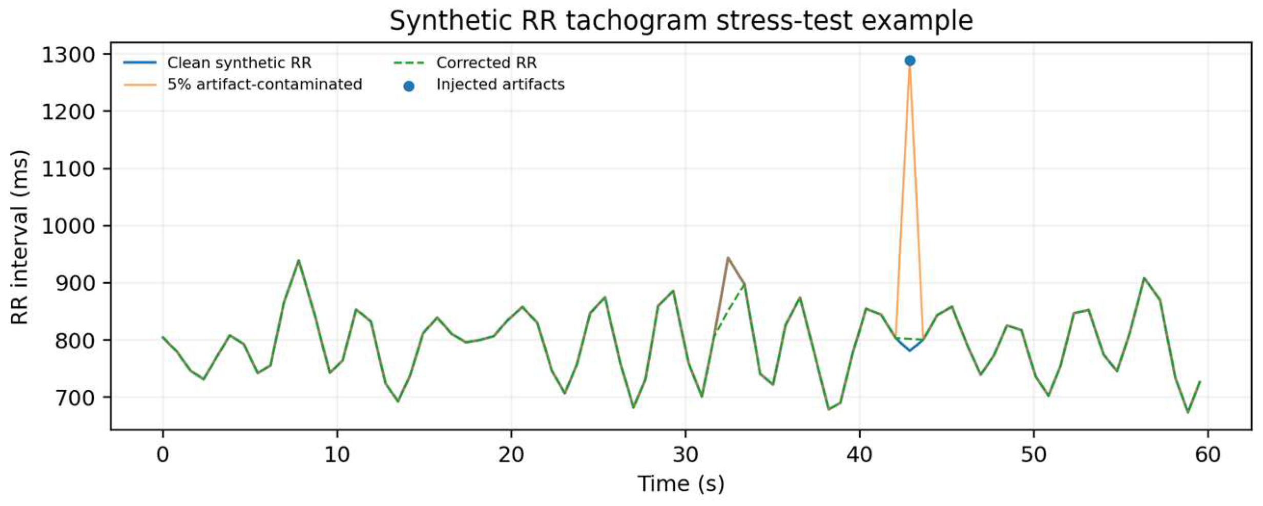
For each 10 min tachogram, HFD, DFA α, and finite-time divergence were calculated from the first 2, 5, and 10 min. The 5 min segment was additionally contaminated at 1% and 5% artifact burdens by randomly replacing selected intervals with premature-like (×0.55) or missed-beat-like (×1.65) values. A prespecified correction rule flagged intervals differing by more than 20% from the local four-neighbor median and replaced the flagged values by linear interpolation between valid neighbors. Both raw contaminated and corrected series were analyzed. These artifacts are algorithmic stressors and are not intended to reproduce the full morphology of ectopy or detector failure.

2.10.3. Signal-Level Performance Measures

Primary signal-level settings were HFD kmax = 10, DFA scales 4–16, and finite-time divergence m = 3, τ = 1, Theiler window = 10, horizon = 20, slope fit over steps 1–10. Results are reported as medians with empirical 2.5th–97.5th percentiles. Paired percentage deviations were calculated relative to the clean 5 min segment. Prespecified sensitivity analyses used HFD kmax = 6, 10, and 15; DFA scale ranges 4–16, 4–32, 8–32, and 8–64; divergence m = 2–4; and τ = 1–3. The divergence fit-quality criterion was R² ≥ 0.90. The analysis was designed to identify numerically fragile settings rather than select a post hoc optimum [27,29].

3. Results

3.1. Worked Synthetic Dataset and Target Calibration

The worked dataset contains 48 explicitly synthetic records. Context variables were generated with a target mean age of 52.31 years, 87.5% of records were designated as female, mean symptom duration was 6.79 years, mean BMI was 28.20 kg/m², sleep-disorder indicators were present in 68.8% of records, and anxiety/depression indicators in 66.7%. These values are generator settings rather than observed epidemiological characteristics. Table 2 lists the metric-level distributional targets.

3.2. Worked Example: Simulated Clinical-Scale Outcomes

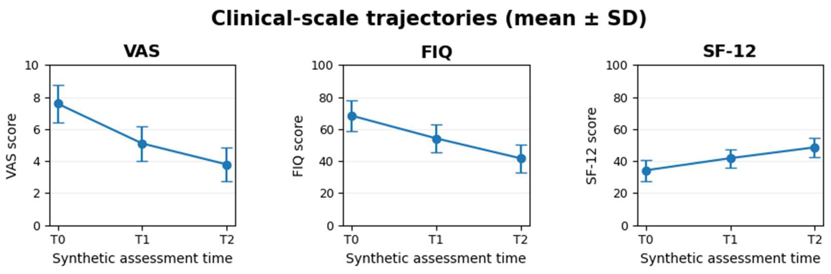
Within the fixed-seed, moment-matched synthetic dataset, VAS changed from 7.59 ± 1.18 at T0 to 3.79 ± 1.07 at T2, FIQ from 68.40 ± 9.70 to 41.70 ± 8.67, and SF-12 from 34.20 ± 6.50 to 48.60 ± 5.99. The corresponding improvement-oriented changes were 3.80 for VAS (T0–T2), 26.70 for FIQ (T0–T2), and 14.40 for SF-12 (T2–T0). These values were imposed by the generator and moment-matching procedure to illustrate reporting; they are not observed improvements or empirical treatment effects (

Table 3. Worked synthetic clinical-scale variables and simulated longitudinal changes. Positive changes are coded toward the prespecified simulated improvement direction and must not be interpreted as observed clinical improvement.

Outcome	T0	T1	T2	Improvement-Oriented Change (95% CI)	Cohen dz
VAS	7.59 ± 1.18	5.10 ± 1.07	3.79 ± 1.07	3.80 [3.39, 4.21]	2.67
FIQ	68.40 ± 9.70	54.20 ± 8.88	41.70 ± 8.67	26.70 [23.86, 29.54]	2.73
SF-12	34.20 ± 6.50	41.79 ± 5.76	48.60 ± 5.99	14.40 [12.51, 16.29]	2.21

).

Separate panels retain the original units of VAS, FIQ, and SF-12. No cross-scale normalization, weighting, or composite recovery scores are used (Table 3).

3.3. Worked Example: Simulated Nonlinear HRV Metrics

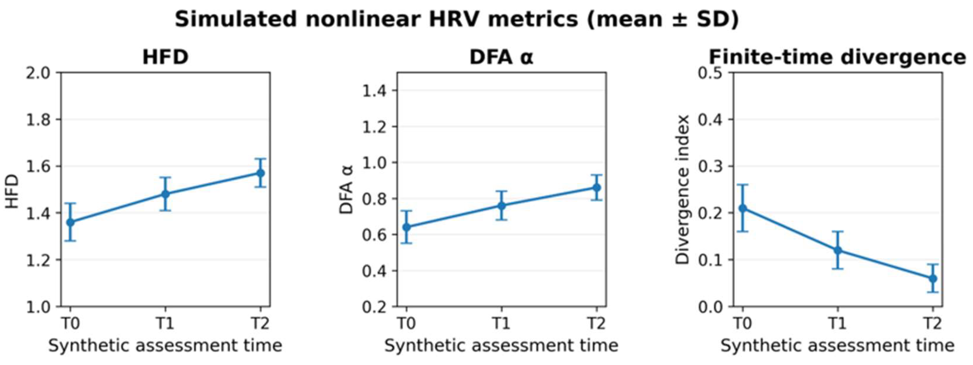
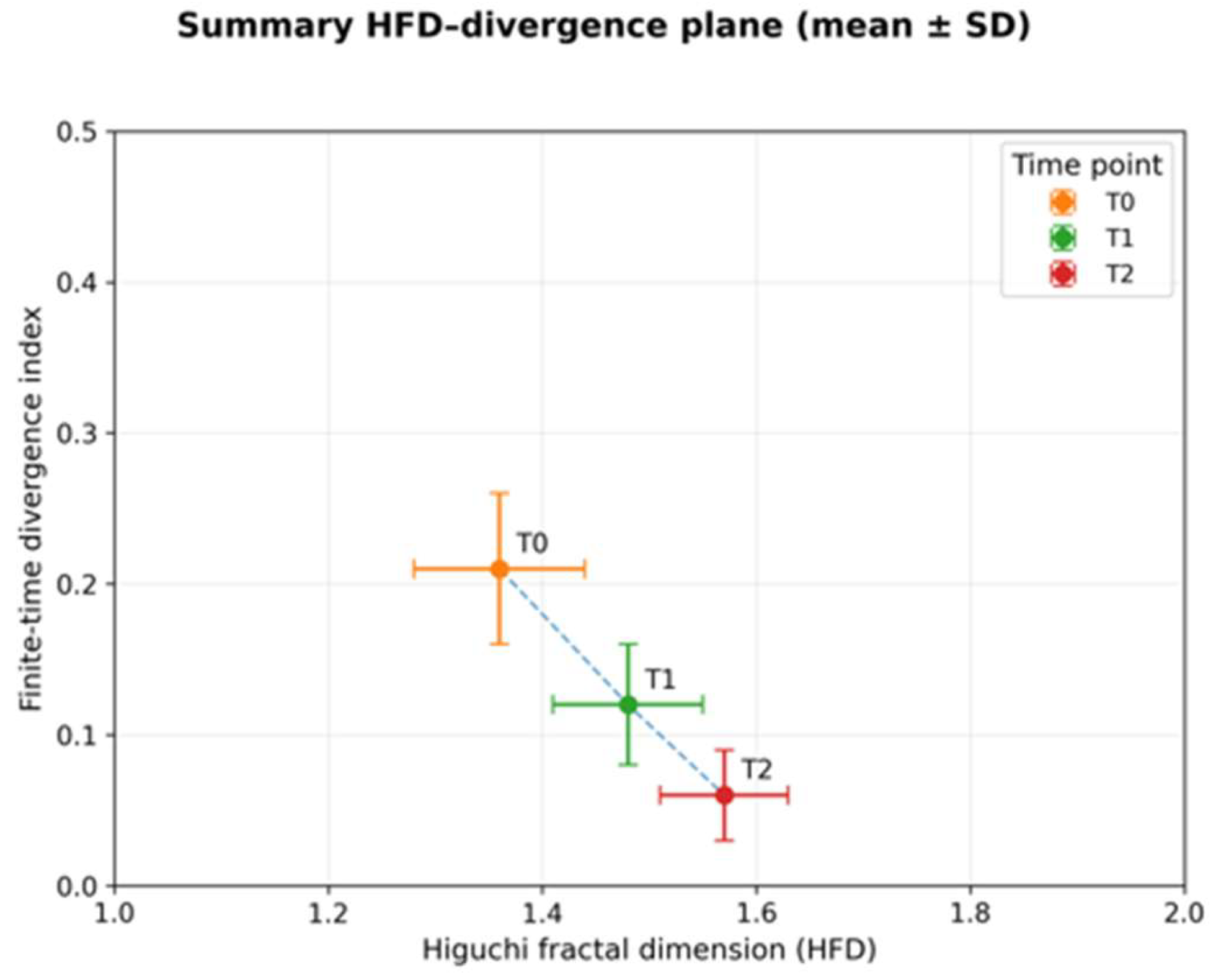
The moment-matched nonlinear targets changed from 1.36 ± 0.08 to 1.57 ± 0.06 for HFD, from 0.64 ± 0.09 to 0.86 ± 0.07 for DFA α, and from 0.21 ± 0.05 to 0.06 ± 0.03 for the finite-time divergence index. These are simulated metric-level values, not estimates computed from RR recordings (

Table 4. Worked synthetic nonlinear outcomes. Positive values denote change in the prespecified improvement-oriented direction.

Metric	T0	T1	T2	Improvement-Oriented Change (95% CI)	Cohen dz
HFD	1.36 ± 0.08	1.48 ± 0.07	1.57 ± 0.06	0.21 [0.19, 0.23]	2.96
DFA α	0.64 ± 0.09	0.76 ± 0.08	0.86 ± 0.07	0.22 [0.19, 0.25]	2.23
Finite-time divergence	0.21 ± 0.05	0.12 ± 0.04	0.06 ± 0.03	0.15 [0.14, 0.16]	2.95

).

Error bars denote standard deviations. The displayed values are simulated metric-level summaries and were not computed from empirical RR interval recordings.

3.4. Worked Example: Correlations Between Simulated Clinical and Nonlinear Changes

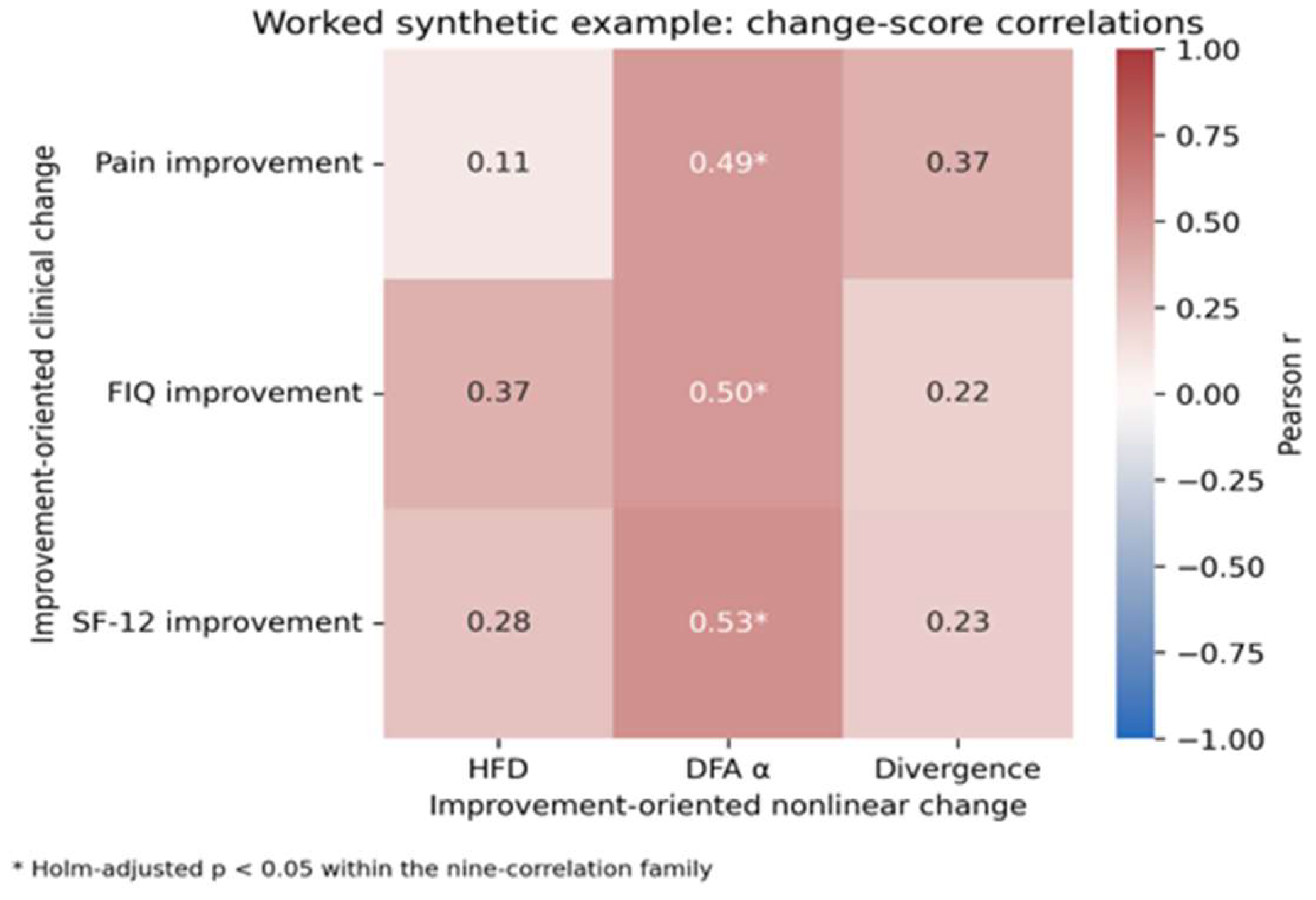
The nine correlations between simulated clinical-scale changes and simulated nonlinear metric changes are presented solely as methodological analysis examples. For this particular random seed, three correlations remained significant after Holm correction, while the others did not. This variability is expected with n = 48 and is summarized across 1000 replications in Section 3.6 (

Table 5. Worked synthetic correlations between improvement-oriented clinical and nonlinear change scores.

Association	r (95% CI)	Raw p	Holm-Adjusted p
Pain improvement vs. HFD increase	0.11 [−0.18, 0.38]	0.465	0.465
Pain improvement vs. DFA α increase	0.49 [0.24, 0.68]	4.03 × 10−4	0.003
Pain improvement vs. Divergence reduction	0.37 [0.09, 0.59]	0.010	0.053
FIQ improvement vs. HFD increase	0.37 [0.10, 0.59]	0.009	0.053
FIQ improvement vs. DFA α increase	0.50 [0.25, 0.69]	3.02 × 10−4	0.002
FIQ improvement vs. Divergence reduction	0.22 [−0.07, 0.47]	0.137	0.351
SF-12 improvement vs. HFD increase	0.28 [−0.00, 0.53]	0.051	0.204
SF-12 improvement vs. DFA α increase	0.53 [0.30, 0.71]	9.07 × 10−5	8.16 × 10−4
SF-12 improvement vs. Divergence reduction	0.23 [−0.06, 0.48]	0.117	0.351

and Table S2).

The heatmap illustrates only one draw from the calibrated generator. It does not establish causal direction, physiological coupling, prognostic utility, or biomarker validity.

3.5. Worked Example: HFD-Divergence Plane

The two-dimensional display shows the imposed shift towards higher HFD and lower divergence across the three synthetic time points. No zones, thresholds, clusters, or physiological states were prespecified or inferred.

The separation among time points reflects the scenario’s encoded mean structure and should not be interpreted as observed recovery trajectories or as evidence of physiological coupling.

3.6. Monte Carlo Stability and Negative-Control Scenarios

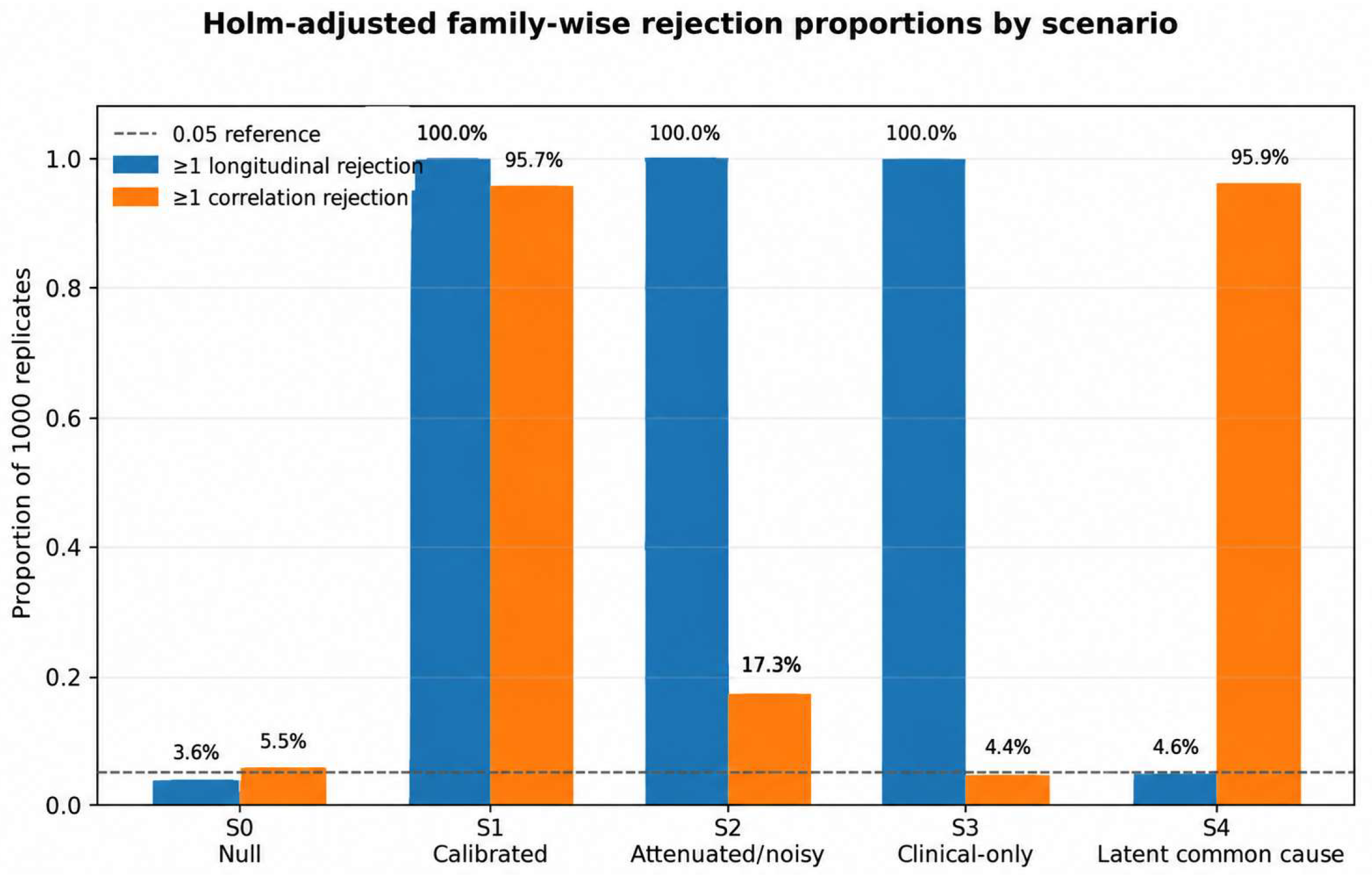
Across 1000 replications, the strict null scenario produced at least one Holm-adjusted rejection in 3.6% of longitudinal families (MCSE 0.6%) and 5.5% of correlation families (MCSE 0.7%). All six longitudinal changes were detected in the calibrated and attenuated/noisy scenarios, whereas only the three simulated clinical-variable changes were typically detected in the clinical-only scenarios.

At least one change correlation was detected in 95.7% of calibrated replicates, 17.3% of attenuated/noisy replicates, 4.4% of clinical-only replicates, and 95.9% of latent common cause replicates. The calibrated scenario’s median cross-domain r values were 0.32–0.40, with broad empirical 2.5th–97.5th percentile ranges. The similarity between S1 and S4 demonstrates that high detection alone cannot distinguish encoded coupling from an unmeasured common cause (

Table 6. Monte Carlo operating characteristics across 1000 replicates per scenario (n = 48 per replicate).

Scenario	≥1 Longitudinal Rejection	≥1 Correlation Rejection	Mean 95% CI Coverage (Change/r)	Interpretation
S0 Null	3.6% (MCSE 0.6%)	5.5% (MCSE 0.7%)	95.1%/94.7%	Family-wise false-positive control
S1 Calibrated	100.0% (MCSE 0.0%)	95.7% (MCSE 0.6%)	94.9%/95.3%	Expected statistical recovery of the prespecified encoded structure
S2 Attenuated/noisy	100.0% (MCSE 0.0%)	17.3% (MCSE 1.2%)	94.8%/95.1%	Lower correlation sensitivity
S3 Clinical-only	100.0% (MCSE 0.0%)	4.4% (MCSE 0.6%)	94.8%/95.0%	Clinical-HRV dissociation
S4 Latent common cause	4.6% (MCSE 0.7%)	95.9% (MCSE 0.6%)	95.0%/95.0%	High marginal correlation without direct mechanism

and Table S3).

Mean 95% confidence interval coverage ranged from 94.8% to 95.1% for mean changes and from 94.7% to 95.3% for correlations across scenarios. These results verify the implementation under the stated generator; they do not validate the biological assumptions or provide clinical evidence. MCSE values in Table 6 and Table S3 are expressed in percentage points.

3.7. Signal-Level Verification and Robustness Results

The canonical checks recovered the expected limiting behavior of the implemented algorithms. HFD was 1.029 for the smooth sinusoid and had a median of 1.999 [1.983, 2.014] across 200 white-noise realizations. For white noise, the median DFA exponent was 0.584 [0.533, 0.648] over scales 4–16 and 0.522 [0.467, 0.579] over scales 4–64, demonstrating the expected finite-scale upward bias of short-range DFA. The logistic-map divergence benchmark was 0.694 with a median R² ≈ 1.000, closely matching the theoretical ln(2) = 0.693. Thus, the code recovered known benchmark behavior while also showing that a numerically correct implementation does not guarantee setting-independent estimates (

Table 7. Canonical signal-level verification of the nonlinear metric implementations.

Benchmark	Expected Behavior	Observed Result	Interpretation
Smooth sinusoid, HFD	≈1	1.029	Correct smooth curve limit
Gaussian white noise, HFD	≈2	1.999 [1.983, 2.014]	Correct irregular-signal limit
Gaussian white noise, DFA 4–16	α = 0.5	0.584 [0.533, 0.648]	Short-scale upward bias
Gaussian white noise, DFA 4–64	α = 0.5	0.522 [0.467, 0.579]	Closer to asymptotic target
Logistic map r = 4, divergence	ln(2) = 0.693	0.694; R2 ≈ 1.000	Correct deterministic benchmark

and Table S5).

In the 120 McSharry-inspired RR replicates, median HFD values were 1.910, 1.902, and 1.904 at 2, 5, and 10 min, respectively; median DFA values were 0.812, 0.811, and 0.811; and median divergence values were 0.080, 0.096, and 0.103. Relative to clean 5 min segments, the median absolute paired deviation at 2 min was 1.45% for HFD, 8.69% for DFA, and 18.04% for divergence; at 10 min it was 0.67%, 3.82%, and 7.41%, respectively. Thus, recording length affected the finite-time divergence estimate more strongly than HFD in this generator.

Injected artifacts produced metric-specific distortions. At 5% artifact burden, median raw HFD increased by 2.29% and median raw DFA decreased by 18.69% relative to the clean series. After the prespecified correction, median absolute deviations from the clean series were 0.93% for HFD, 6.16% for DFA, and 9.16% for divergence. At 1% artifact burden, the corresponding median absolute deviations after correction were 0.37%, 3.04%, and 4.13%. The correction, therefore, reduced some artifact effects but did not restore all nonlinear estimates exactly (

Table 8. Nonlinear metric estimates across RR recording-length and artifact stress conditions (120 replicates; median [2.5th, 97.5th percentile]).

Condition	HFD	DFA α	Finite-Time Divergence	Divergence R2 ≥ 0.90
2 min clean	1.910 [1.800, 1.998]	0.812 [0.569, 1.070]	0.080 [0.048, 0.110]	0%
5 min clean	1.902 [1.857, 1.960]	0.811 [0.670, 0.930]	0.096 [0.079, 0.112]	0%
10 min clean	1.904 [1.887, 1.917]	0.811 [0.781, 0.833]	0.103 [0.093, 0.116]	0%
1% artifacts, raw	1.918 [1.875, 1.966]	0.742 [0.614, 0.863]	0.093 [0.077, 0.110]	0%
1% artifacts, corrected	1.895 [1.844, 1.943]	0.840 [0.721, 0.949]	0.093 [0.076, 0.106]	0%
5% artifacts, raw	1.947 [1.919, 1.978]	0.658 [0.537, 0.754]	0.095 [0.077, 0.113]	0%
5% artifacts, corrected	1.880 [1.838, 1.933]	0.860 [0.743, 0.973]	0.088 [0.069, 0.102]	0%

and Table S6).

Parameter sensitivity was substantial. Across the clean 5 min replicates, median HFD changed from 1.830 at kmax = 6 to 1.902 at kmax = 10 and 1.987 at kmax = 15. Median DFA changed from 0.811 for scales 4–16 to 0.510 for 4–32, 0.326 for 8–32, and 0.177 for 8–64, consistent with scale-dependent structure in the LF/HF tachogram. Median divergence was 0.060, 0.096, and 0.102 for m = 2, 3, and 4, respectively, and 0.096, 0.067, and 0.033 for τ = 1, 2, and 3. Importantly, none of the primary 1–10-step divergence fits in the RR stress test met the prespecified R² ≥ 0.90 quality criterion. This failure is reported rather than optimized away and supports treating the divergence metric as exploratory until validated on empirical RR data. The parameter sensitivity medians are provided in Table S4.

In Figure 7, the solid brown/orange line represents the 5% artifact-contaminated synthetic RR tachogram. It is plotted over the original clean RR series to illustrate the effect of the deliberately injected artifacts; where the two series overlap, the superposition may appear brown/orange. The green dashed line shows the corrected series, and the markers indicate the injected artifacts.

4. Discussion

This simulation-based methodological study separates two questions: whether the statistical integration workflow behaves as expected under controlled data-generating mechanisms, and whether the nonlinear descriptors are numerically recoverable and robust when computed from signals. The signal-level layer addresses the second question directly, while preserving the boundary against clinical inference. Standard paired tests, Pearson correlations, Holm correction, and the individual nonlinear descriptors are not presented as novel methods.

The worked synthetic dataset demonstrates how clinical scales and nonlinear metrics can be displayed together, but its means and standard deviations were deliberately calibrated. Consequently, large changes and small p values in that example are expected consequences of the data-generating process. The Monte Carlo scenarios, rather than the single dataset, are the appropriate basis for evaluating the statistical workflow.

HFD should not be interpreted as a monotonic health score. The RR interval stress test showed little median duration drift but clear kmax dependence and measurable artifact sensitivity, consistent with known concerns about the perturbation and parameter dependence of Higuchi estimates [29]. The same caution applies to DFA α: although median estimates at 2, 5, and 10 min were similar under this generator, they changed markedly with scale range and artifact contamination, and the canonical white-noise benchmark showed upward bias over 4–16 samples [27].

The finite-time divergence index was the most fragile of the three descriptors in the RR stress test. It changed with recording duration, embedding dimension, and delay, and the prespecified R² ≥ 0.90 fit-quality criterion was not satisfied under the primary 1–10-step fit. This finding reinforces the decision not to label the measure as the largest Lyapunov exponent and argues against the physiological interpretation of a single setting-dependent slope from short RR series without empirical validation.

The comparison of S1 with S2 and S3 shows that correlations are unstable when the embedded signal is weaker or when clinical and nonlinear changes are generated independently. This directly addresses the circularity of calibrating one synthetic dataset to reproduce expected associations.

S4 provides an additional caution: a latent shared factor produced correlation rejections almost as frequently as in the calibrated coupling scenario, despite the absence of mean change. A marginal correlation between clinical and HRV changes therefore cannot identify a physiological mechanism.

With 48 synthetic records and several covariates, regression coefficients would be too unstable for clinical prediction and would largely reflect assumptions encoded by the generator. Future real-data models require an a priori sample-size calculation, internal validation, and an independent external cohort.

Medication use, sleep quality, psychological state, activity level, respiratory pattern, pain flare, body position, and circadian variation may influence short-term HRV. These factors must be measured rather than inferred. In particular, respiration should be recorded or controlled before changes are interpreted as evidence of altered autonomic organization.

Limitations

First, no real RR recordings or patient-level physiological signals were analyzed. The new signal-level extension uses controlled synthetic signals and McSharry-inspired RR tachograms, so it can test numerical implementation and robustness within known generators but cannot reproduce the full measurement error, ectopic morphology, respiration, nonstationarity, device behavior, or test–retest variability of empirical recordings.

Second, the calibrated scenario intentionally embeds the target shifts and the shared correlation structure. Recovery of these targets is circular by design and should be interpreted only as a reproducibility check.

Third, n = 48 was retained for the worked example and was not justified as a clinical sample size. Although 1000 replicates characterize the workflow under the generator, these do not compensate for the absence of empirical data.

Fourth, respiration was not measured because no physiological acquisition occurred. The latent common cause scenario demonstrates vulnerability to respiratory or other unmeasured influences but cannot quantify their real magnitude.

Fifth, the nonlinear parameter settings remain reference choices rather than validated fibromyalgia-specific settings. The added stress test demonstrates, rather than resolves, this limitation: HFD, DFA, and divergence changed with kmax, scale range, embedding dimension, and delay, and the primary divergence fit failed its prespecified quality threshold. Future work must therefore define settings based on empirical reliability, sensitivity, surrogate behavior, and external validation rather than on favorable simulated results.

Finally, the simulation uses bounded Gaussian metric-level models. Real clinical and HRV data may be skewed, heteroscedastic, missing not at random, clustered, or affected by dropout. Additional generators and empirical validation are required before generalizing the operating characteristics.

A future validation program should prospectively recruit a cohort of patients with fibromyalgia and an appropriate control group, record respiration and key confounders at standardized visits, archive raw and corrected RR series, prespecify nonlinear settings and multiplicity families, report adherence and exclusions, perform long-term follow-up, and confirm findings in an independent cohort.

Accordingly, the present findings should be interpreted as operating characteristics of a dual-layer simulation framework: Layer A characterizes the statistical workflow under explicit metric-level generators, whereas Layer B characterizes the numerical behavior of the nonlinear algorithms under controlled synthetic signal conditions. Neither layer establishes biological validity, treatment responsiveness, or clinical usefulness.

5. Conclusions

This dual-layer simulation study provides a reproducible framework for presenting simulated clinical scales and nonlinear HRV metrics while testing signal processing behavior separately. Canonical benchmarks support the numerical implementation, whereas synthetic RR interval stress tests show that artifact burden, recording duration, scale range, kmax, embedding dimension, and delay can materially alter nonlinear-estimate values. The study does not demonstrate functional recovery, autonomic reorganization, rehabilitation efficacy, clinical thresholds, or biomarker performance.

The metric-level Monte Carlo results show family-wise false-positive control under the strict null, lower correlation detection when signals are attenuated or dissociated, and vulnerability to a latent common cause. The signal-level results further show that well-behaved downstream statistics do not guarantee stable or identifiable upstream nonlinear metrics when signals are shortened, contaminated, or analyzed with alternative settings. In particular, the primary finite-time divergence fit requires further methodological development before empirical use.

Prospective studies using real RR recordings, respiratory monitoring, appropriate controls, prespecified preprocessing, larger samples, long-term follow-up, and independent external validation are required before nonlinear HRV metrics can be considered for use in fibromyalgia rehabilitation.