4.1. Benchmark Model Comparison and Selection
Five standard regression algorithms were chosen as benchmark algorithms: random forest (RF), support vector regression (SVR), XGBoost, multilayer perceptron (MLP), and TabNet. These models are various learning processes, such as bagging-based decision trees, kernel-based regression, boosting-based decision trees, traditional neural networks, and attention-based learning with structured tabular data. Their performance was contrasted to determine an appropriate backbone model to learn the nonlinear relationship between external strain responses and corrosion defect geometry.
The same dataset, training–testing partition, and preprocessing procedure as in
Section 3 were used to evaluate all benchmark models. The input variables were tank wall thickness, hydrostatic pressure, maximum circumferential strain, and strain concentration factor, and corrosion depth and pit diameter were considered the two target variables. Each of the methods was tested within the same two-target regression framework. The preprocessing parameters were only obtained using the training set and then applied to the testing set to avoid information leakage.
Since the predictive performance of each model depends on its hyperparameter configuration, BO was applied consistently to all five benchmark models. BO builds a surrogate model of the validation objective and applies an acquisition function to identify promising hyperparameter combinations, making it suitable for computationally expensive black box optimization [
29]. For each model, BO was conducted for 50 iterations using five-fold cross-validation on the training subset. After BO, each model was refitted using the complete training subset with the selected hyperparameters and evaluated once on the held-out testing subset. The Expected Improvement acquisition function was used to select the hyperparameter combination evaluated at each iteration. The optimization objective was to minimize the mean cross-validation root mean square error (RMSE) averaged across the standardized corrosion depth output d and the log-transformed and standardized pit diameter output L. The hyperparameter combination with the lowest objective value was selected. The testing subset was excluded from hyperparameter optimization and was used only for the final performance evaluation.
Table 4 summarizes the hyperparameter search spaces and the values selected by BO.
The mean absolute error (MAE), RMSE, and coefficient of determination (R
2) were used to assess the optimized models. MAE explains the mean size of the prediction errors, and RMSE gives more weight to the large errors. Lower MAE and RMSE values indicate better prediction accuracy. R
2 value explains the relationship between the predicted and actual values with a value nearer to 1 showing better performance of the model. The three measures were computed individually on the corrosion depth and pit diameter once the predicted measures were transformed back to their physical units. The testing performance of the five optimized benchmark models is summarized in
Table 5.
TabNet was the best overall predictor in the conditions studied, with the lowest MAE and RMSE values and the highest R2 values of corrosion depth and pit diameter. Thus, TabNet was chosen as the most appropriate model to be used in the current corrosion defect inversion task.
4.2. Development and Evaluation of the Dual-Output MHA-TabNet Model
According to the benchmark comparison in
Section 4.1, BO-TabNet was chosen as the backbone model to be developed. TabNet is a deep learning model that works with structured tabular data. Recent reviews and enhanced TabNet variants have demonstrated that nonlinear representation learning can be achieved by sequential attention and step-wise feature selection, and still maintain some level of interpretability [
30,
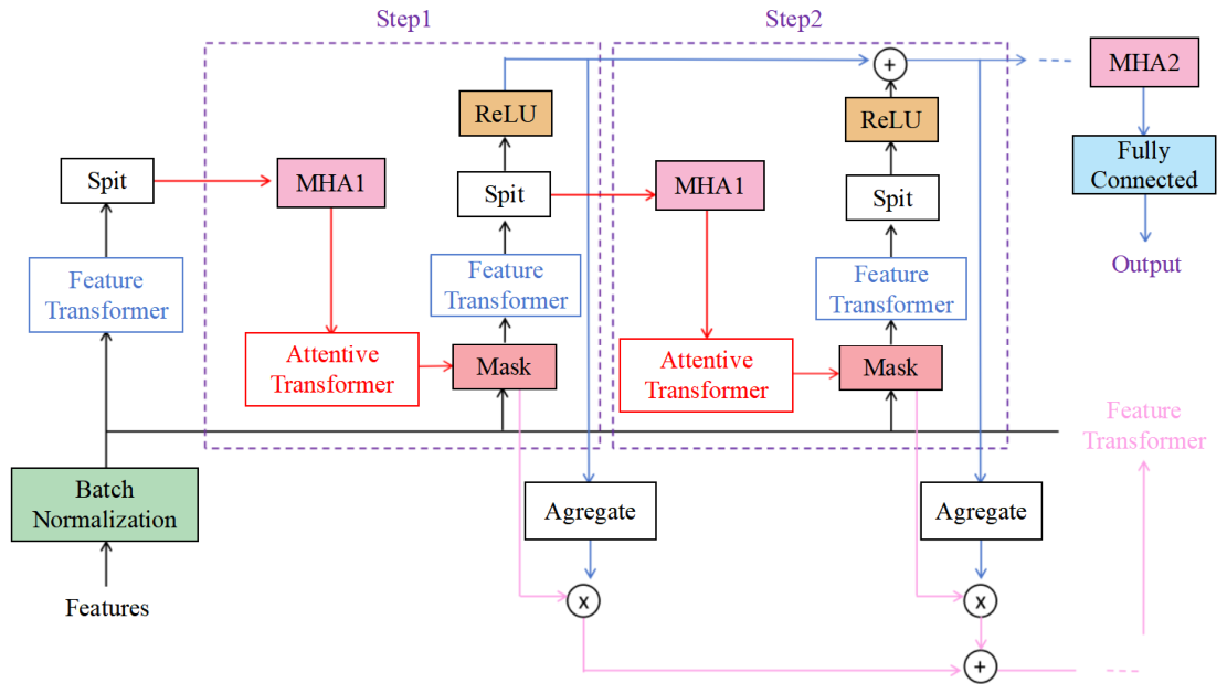
31]. An Attentive Transformer is used at every decision step to produce a sparse feature mask to choose the variables that are important to the decision at hand, and a Feature Transformer transforms the chosen variables into higher-order representations.
Even though TabNet is capable of dynamically choosing influential features, its Feature Transformer primarily uses fully connected layers and nonlinear activation functions. The sparse mask selects the variables to be kept at each decision step but is not very effective in explicitly modeling joint interactions between tank wall thickness, hydrostatic pressure, maximum circumferential strain, and SCF. This constraint can limit the modeling of the highly coupled nonlinear interaction between strain responses and corrosion geometry.
The feature-interaction methods that rely on attention to tabular data have shown that multiple heads can learn complementary relationships between variables and informative feature weighting [
32]. To enhance cross-feature interactions, MHA modules were introduced into the TabNet architecture. Scaled dot-product attention is defined as
where
,
, and
are the query, key, and value matrices, respectively, and
is the dimension of the key vectors.
The scaling term restricts overly large dot-product values and enhances the numerical stability of the Softmax operation.
For a mini-batch containing
B samples, the standardized input tensor has a shape of
B × 4, with the four columns corresponding to tank wall thickness, hydrostatic pressure, maximum circumferential strain, and SCF. At each decision step, the output of the Feature Transformer is divided by the Split operation into a decision representation and an attention representation, with dimensions of
B ×
na and
B ×
na, respectively. As illustrated in
Figure 12, MHA1 is applied to the attention branch between the Split operation and the Attentive Transformer. The attention representation is converted into four ordered feature-associated tokens through feature-specific linear projections, with each token corresponding to one input variable. Using the fixed embedding dimension of 64, the resulting MHA1 input tensor has a shape of
B × 4 × 64. With the two attention heads selected by BO, each head has an embedding dimension of 32. After head separation, the query, key, and value tensors each have a shape of
B × 2 × 4 × 32. The outputs of the attention heads are concatenated and linearly transformed as
In Equation (17),
X denotes the token tensor supplied to the corresponding MHA module. Equation (17) is applied separately to MHA1 and MHA2, and the two modules do not share weights. For MHA1, the multi-head output retains a shape of
B × 4 × 64 and is subsequently projected back to a representation with a shape of
B ×
na. The resulting representation is passed to the Attentive Transformer to generate the sparse feature mask for the next decision step. At the global level, the decision representations produced by the four decision steps are treated as four ordered step-wise tokens. Each decision representation, with a shape of
B ×
na, is projected to 64 dimensions, resulting in an MHA2 input tensor with a shape of
B × 4 × 64. With two attention heads, the corresponding query, key, and value tensors each have a shape of
B × 2 × 4 × 32. MHA2 captures the dependencies among the decision-step representations. Its output is summed across the four step-wise tokens and passed to a fully connected regression layer with two output nodes:
where
and
denote the predicted corrosion depth and pit diameter, respectively. The two output nodes share the fused representation produced by MHA2, allowing for the model to learn information common to both targets while retaining target-specific predictions [
33]. Consequently, corrosion depth and pit diameter are predicted simultaneously by a single shared model rather than by two independently trained neural networks.
The BO procedure outlined in
Section 4.1 was used to determine the hyperparameters of MHA-TabNet. Since the modified architecture added attention-specific parameters, the search space had the number of attention heads and the attention dropout rate besides the original TabNet parameters. The hyperparameter search spaces and the values selected through BO are listed in
Table 6. The optimized model is henceforth called BO-MHA-TabNet.
To compare the baseline and modified architectures under the same model development procedure, the BO-TabNet model selected in
Section 4.1 was compared with BO-MHA-TabNet. The training and testing samples, preprocessing procedure, BO strategy, and evaluation metrics were the same in all models. Their results on the same held-out testing set are summarized in
Table 7.
Table 7 indicates that BO-MHA-TabNet performed better than BO-TabNet in the inversion of corrosion depth and pit diameter. For corrosion depth, the testing MAE and RMSE decreased from 0.248 and 0.354 mm to 0.226 and 0.257 mm, respectively, while R
2 increased from 0.9263 to 0.9612. For pit diameter, the MAE decreased from 28.336 to 24.252 mm, the RMSE decreased from 41.612 to 32.505 mm, and R
2 increased from 0.8979 to 0.9377.
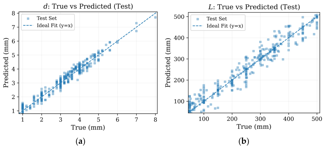
The regression fitting results of BO-MHA-TabNet on the testing set are shown in
Figure 13. The actual and predicted values are represented by the horizontal and vertical coordinates, respectively, and the ideal prediction is represented by the dashed
y =
x line. The predictions of corrosion depth are closely distributed around the ideal line. The predictions of pit diameter also show good overall agreement with the actual values, although a relatively broader and more scattered distribution is observed compared with corrosion depth, with no evident systematic deviation over the investigated range.
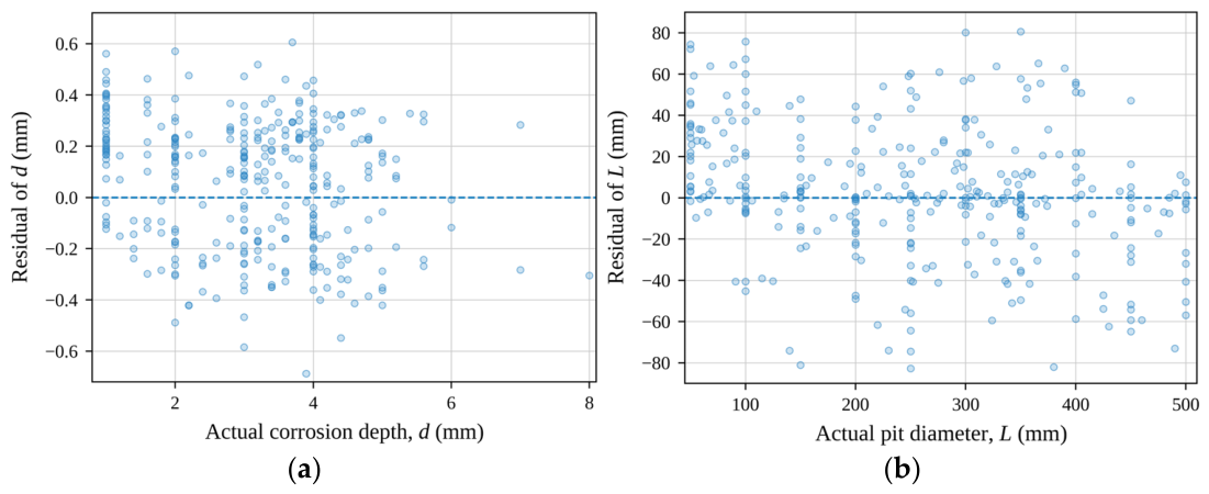
Figure 14 shows the prediction residuals with respect to the actual corrosion depth and pit diameter. The residuals of corrosion depth are mainly distributed around zero and remain relatively stable over the investigated range. For pit diameter, the residuals are also distributed around zero, with a somewhat wider dispersion than that of corrosion depth but without an evident increase with diameter. As shown in
Table 8, the absolute prediction errors of both outputs remain generally stable across the different value intervals, whereas the normalized errors are more pronounced for smaller defects. Here, normalized mean absolute error (NMAE) is calculated as the interval MAE divided by the mean actual value within the corresponding interval. The NMAE reaches 13.79% for corrosion depths of 1–3 mm and 23.86% for pit diameters of 50–200 mm but decreases to 4.09% and 6.27% in the largest depth and diameter intervals, respectively. These results indicate that the global average metrics should be interpreted together with the actual defect dimensions, particularly for smaller defects.
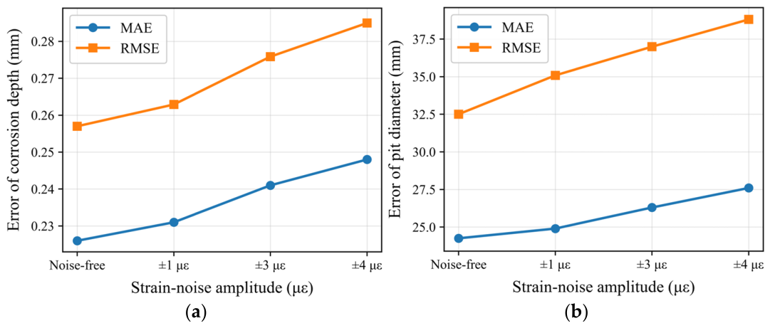
To evaluate the influence of strain measurement uncertainty on the inversion results, bounded random noise was independently introduced into εpit and εref in the testing set. Given the approximate ±1 με strain measurement accuracy of the DH5922N-based acquisition system, disturbance levels of ±1, ±3, and ±4 με were selected to represent nominal, clearly amplified, and conservative upper measurement uncertainties, respectively. For each noise level, the perturbations were sampled uniformly within the corresponding bounds. The strain concentration factor was then recalculated as SCF = εpit/εref, and the perturbed strain features were evaluated using the trained BO-MHA-TabNet model without retraining. Each noise condition was repeated 50 times, and the mean prediction metrics were reported.
As shown in
Figure 15, the prediction performance gradually decreased with increasing strain noise amplitude. For corrosion depth, the MAE increased from 0.226 to 0.231, 0.241, and 0.248 mm, while the RMSE increased from 0.257 to 0.263, 0.276, and 0.285 mm, and R
2 decreased from 0.9612 to 0.9594, 0.9553, and 0.9523. For pit diameter, the MAE increased from 24.252 to 24.900, 26.300, and 27.600 mm, while the RMSE increased from 32.505 to 35.089, 36.995, and 38.807 mm, and R
2 decreased from 0.9377 to 0.9274, 0.9193, and 0.9112. These results indicate that measurement uncertainty gradually reduces prediction accuracy, although the model retains its overall predictive capability within the investigated noise range.
Because BO-TabNet and BO-MHA-TabNet used the same data partition, preprocessing procedure, BO strategy, and evaluation metrics, their testing results can be compared directly. As shown in
Table 7, BO-MHA-TabNet achieved lower MAE and RMSE values and higher R
2 values for both corrosion depth and pit diameter. Although the magnitude of improvement varied between the two targets and across the three metrics, the optimized BO-MHA-TabNet configuration achieved better overall testing performance than BO-TabNet under the present conditions. BO-MHA-TabNet was therefore adopted as the final dual-output corrosion defect inversion model.
4.3. SHAP-Based Interpretation
Although BO-MHA-TabNet achieved high prediction accuracy, its nonlinear internal structure makes it difficult to determine how input variables contribute to the inversion results. The final BO-MHA-TabNet model was thus subjected to SHAP to measure the contribution of each input feature [
34,
35]. SHAP analysis was performed separately for the two model outputs. A positive SHAP value means that the respective feature enhances the predicted corrosion depth or pit diameter compared to the baseline prediction, and a negative value means that it reduces the contribution.
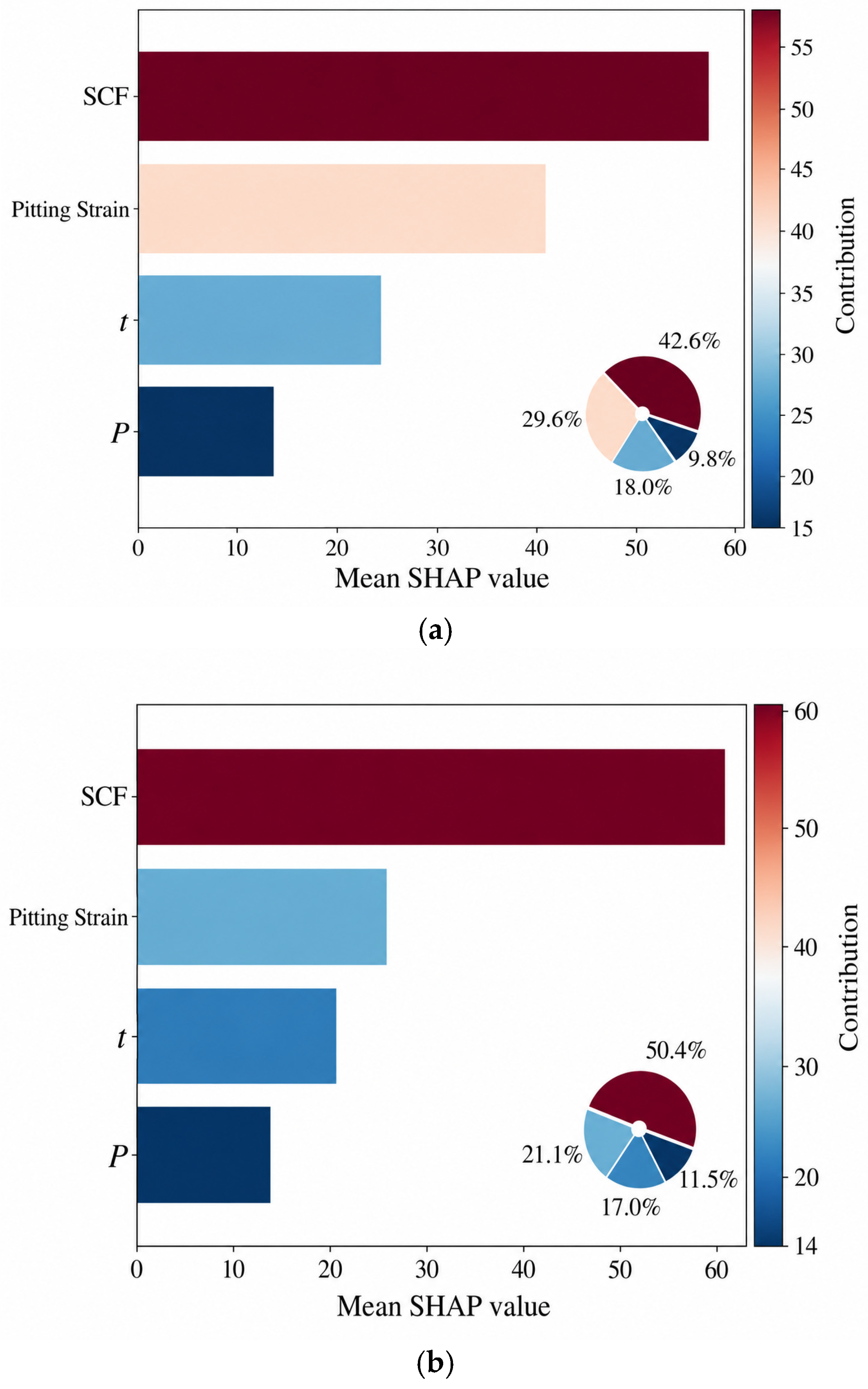
The mean absolute SHAP value was used to assess the global significance of each feature. The feature rankings for the inversion of corrosion depth and pit diameter were generally similar, as indicated in
Figure 16. The most significant feature was the strain concentration factor, which contributed about 42–43% of the total contribution to prediction of corrosion depth and about 50% of the contribution to prediction of pit diameter. The highest circumferential strain was second, with a contribution of about 29–30% and 21–22% to the two outputs, respectively. In comparison, tank wall thickness added about 17–18%, and hydrostatic pressure added about 9–12%.
The prevalence of the two strain response characteristics is in line with the physical nature of the proposed inversion method. The strain concentration factor is the amplification of the local response compared to an intact region at the same elevation. Localized thinning of the wall disrupts the circumferential load transfer path and enhances deformation around the corrosion pit, rendering SCF sensitive to defect geometry variations. The maximum circumferential strain is the absolute measure of local deformation and is a direct measure of the decrease in local stiffness. The structural and loading context is given by tank wall thickness and hydrostatic pressure, but some of their effect is already represented by the two strain response features. Their SHAP contributions are thus smaller yet still needed to differentiate similar strain responses produced under varying structural and loading conditions.
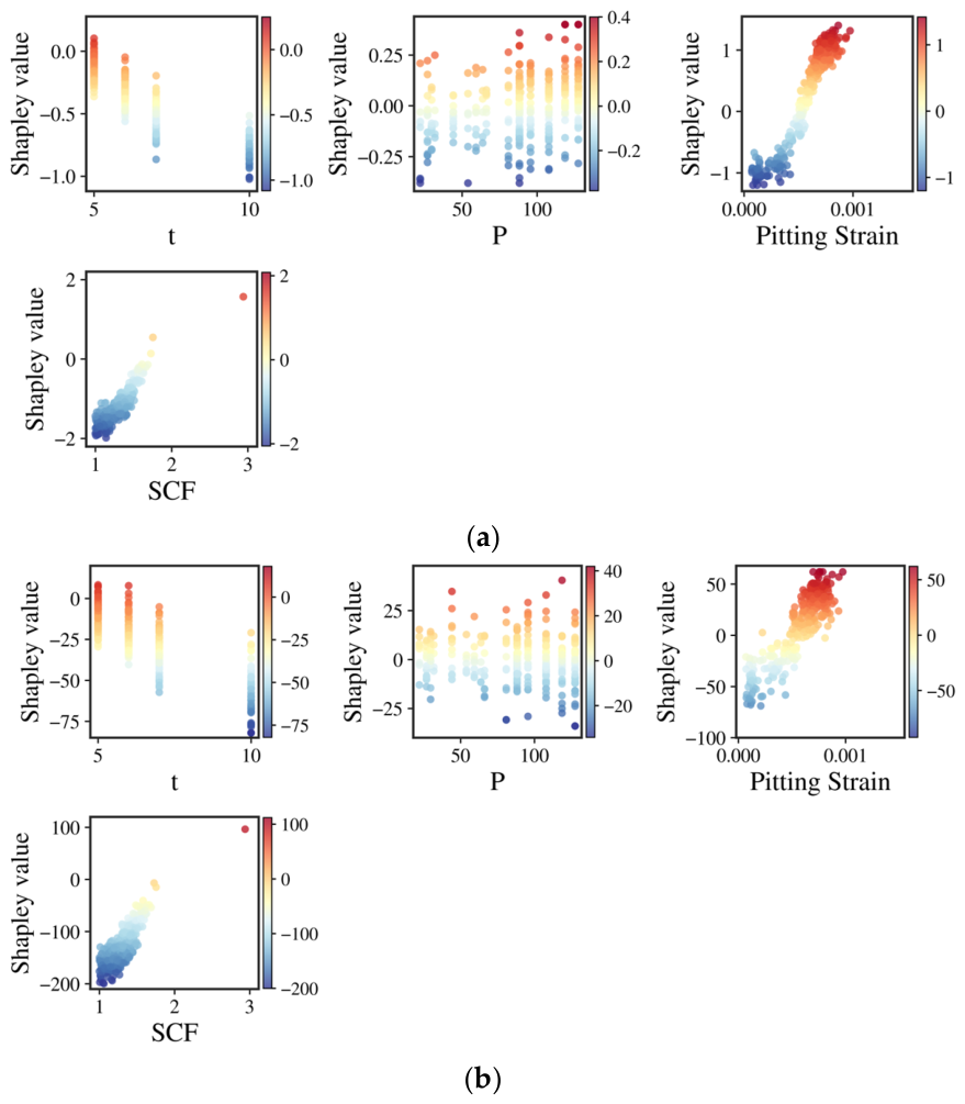
The nonlinear dependence of the four inputs is also demonstrated by the SHAP dependence plots in
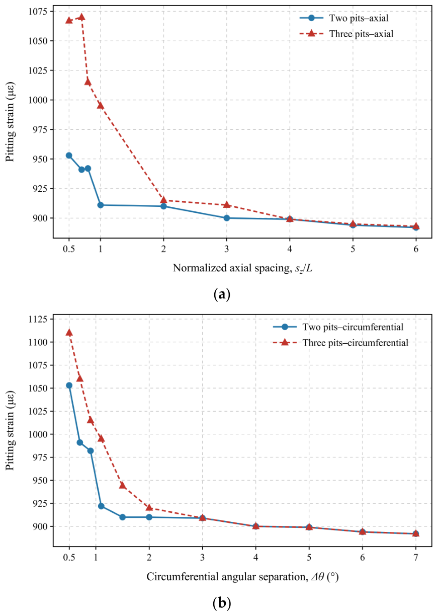
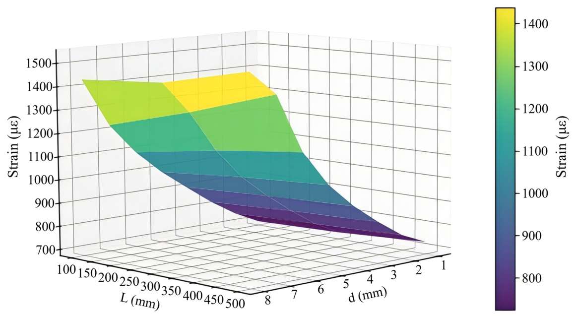
Figure 17. The points are one sample each, and the horizontal axis is the value of the feature, and the vertical axis is the SHAP contribution. With the increase of SCF, between about 1 and 3, the SHAP value of both outputs gradually shifted to positive. This indicates that stronger local strain concentration led the model to predict larger corrosion depth and pit diameter. The maximum circumferential strain also showed a similar increasing trend with higher strain values tending to contribute positively to both inversion results. The SHAP trends are consistent with the mechanical trends observed in the FE sensitivity analysis.
The thickness of tank walls showed a general negative SHAP trend in the data set under study, which means that it was primarily a structural stiffness variable in the model decision process. Hydrostatic pressure had a smaller SHAP range than the two strain response features. Its primary role was to characterize the overall loading level, whereas local amplification caused by defects was better characterized by the maximum circumferential strain and SCF.
In general, the SHAP results indicate that BO-MHA-TabNet mainly uses local strain amplification due to corrosion to predict defect geometry, and tank wall thickness and hydrostatic pressure are complementary structural and loading data. The rankings of feature importance and dependence trends are in line with the local stiffness reduction and strain concentration mechanisms developed in
Section 2. This uniformity enhances the physical plausibility and transparency of the strain-based corrosion defect inversion model. SHAP explains the associations that the model has learned but does not give independent causal evidence; it is used here to ensure that the model decision patterns are consistent with the observed mechanical response.