Predicting Negative Day-Ahead Electricity Prices Across 12 European Bidding Zones: A Gate-Closure-Audited Explainable Machine Learning Framework

Featured Application

The framework can support system and market operators, aggregators, demand-response providers, storage operators and regulators in identifying periods of heightened negative-price risk and market conditions potentially associated with limited absorption of surplus energy. The main model uses information classes audited for regulatory availability before day-ahead gate closure, whereas later wind and solar generation forecasts and market-coupling results are used solely for diagnostic purposes. Implementation requires local calibration, a user-specific cost function and drift monitoring.

Abstract

The growing penetration of variable renewable energy (VRE) is increasing the frequency of very low and negative prices, although these events also depend on demand, transmission capacity, price-regime persistence and flexibility resources. This study examines which pre-auction and diagnostic variables are associated with negative day-ahead prices across European bidding zones, and whether these relationships remain stable over time and transferable across markets. More than 736,000 observations from 12 bidding zones in 2019–2025 were analysed, with sample coverage varying by data completeness. A gate-closure-audited Extreme Gradient Boosting (XGBoost) model achieved moderate risk-ranking performance and positive probabilistic skill in 2024–2025. The strongest pre-auction signals were completed-auction price history, calendar features and structural load relationships. Leave-one-market-out validation showed partial and heterogeneous transferability, supporting local calibration. A separate diagnostic layer revealed market-specific, non-linear associations involving VRE forecasts, residual load and cross-border exchange. Negative prices are therefore interpreted as screening signals for market configurations potentially associated with limited surplus absorption, rather than direct evidence of a flexibility shortfall. The framework separates operational pre-auction prediction from later market diagnosis and provides a reproducible basis for local early-warning applications. All SHAP, ALE and scenario results are interpreted as predictive associations and model diagnostics, not as causal effects or direct measures of physical flexibility.

1. Introduction

1.1. Negative Electricity Prices in Renewable-Dominated Power Markets

The European energy transition is leading to a rapid increase in the share of variable renewable energy (VRE), primarily wind and solar, whilst simultaneously increasing the importance of short-term demand flexibility, storage, controllable generation and cross-border interconnections. Recent assessments of the European market highlight that periods of very low and negative prices are becoming more frequent, as periods of high generation at low marginal cost are not always synchronised with demand and energy absorption capacity [1,2,3,4]. The change in the day-ahead market time unit (MTU) to 15 min, implemented in Europe from 30 September 2025, further increases the resolution of price signals and requires careful comparison of data before and after the change [5].

A negative day-ahead price is a market outcome in which sellers are willing to pay for electricity to be taken off the system. This may reflect the simultaneous occurrence of high supply, low demand, technical constraints on generation units, shutdown and restart costs, support mechanisms or insufficient flexibility. However, a negative price is not automatically synonymous with curtailment: generation reduction is a physical and operational decision, whereas the price results from the market clearing of bids and offers within a bidding zone. Classic analyses of the German market have shown that the negative-price regime should be considered together with wind generation, demand and the structure of system flexibility, rather than as a simple consequence of renewable-energy growth alone [6,7].

The merit-order effect refers to the reduction in wholesale prices by sources with low marginal costs, whilst price cannibalisation concerns the decline in the market value of energy generated by a particular technology when its production coincides temporally with output from the same technology. These two phenomena are interrelated but are not synonymous with negative prices. Research into the market value of VRE has shown that, as the share of wind and solar PV increases, their value factor decreases, particularly when the system does not simultaneously develop flexibility [8,9]. German analyses have also confirmed that higher wind generation lowers price levels and may alter price volatility; however, the direction and strength of this relationship depend on market conditions [10].

From an operational perspective, the mismatch between forecast generation and load, and the system’s ability to shift energy in time or space, is more important than the share of renewable energy sources itself. Negative prices can be regarded as a potential indicator of flexibility-related market stress, but they are not a direct measure of available flexibility or system instability. They point to market configurations in which surplus energy has not been fully absorbed given existing bids, constraints and market design. This approach allows the predicted risk to be examined without attributing the event to a single causal mechanism.

Accordingly, the empirical target in this study is the observable negative-price event, while the broader operational concern is the market configuration associated with limited surplus absorption. We use negative prices as a screening indicator with limited construct specificity: they are directly observable and operationally relevant, but they are neither an econometric instrumental variable nor a validated one-to-one proxy for a flexibility shortage. The framework therefore predicts the market outcome itself and uses later diagnostic variables only to characterise conditions associated with that outcome.

1.2. Residual Load and the Flexibility of Electricity Systems

Forecast residual load, understood as the forecast load minus the forecast wind and solar generation, summarises the relationship between demand and VRE supply. A low or negative residual load means that the remainder of the system must curtail generation, increase consumption, store energy or export the surplus. Under conditions of high VRE penetration, it is not only the level of residual load that matters, but also its ramps, minimum values within short time windows and seasonal and diurnal dynamics.

System flexibility has many dimensions. It encompasses rapid changes in the output of conventional units, storage, flexible demand, sector coupling, cross-border trade and schedule adjustments. The literature has emphasised that minimum generation constraints and start-up costs may contribute to negative prices, whilst appropriately designed storage facilities and demand response can absorb energy surpluses [11,12,13,14]. At the same time, storage does not automatically resolve all issues: its value depends on the price profile, efficiency, power and capacity constraints, and opportunity costs.

The growth of VRE may reduce the market value of wind and solar power, but the scale of this process is not predetermined. Economic analyses indicate that transmission, storage, flexible demand and changes in the generation mix can limit cannibalisation [15,16]. In turn, studies of the Californian market have confirmed different cannibalisation profiles for wind and photovoltaics, which justifies separating VRE components and interactions with the time of day [17].

Flexible electricity demand can also shift consumption toward hours of abundant renewable generation. Recent optimisation research on highway energy systems shows that coordinated EV charging and battery swapping can reshape electricity demand to increase local solar energy utilisation and reduce grid purchases [18]. Although that setting differs from wholesale negative-price forecasting, it illustrates a broader operational mechanism relevant here: controllable loads can absorb variable renewable output when scheduling is responsive to temporal availability.

Cross-border interconnectors play a dual role. They enable the export of local surplus but at the same time transmit the impact of correlated generation from neighbouring markets. Consequently, positive export capacity alone does not guarantee a reduction in the risk of negative prices in every hour. It is necessary to consider the planned net position, scheduled exchange and available capacity in relation to local demand, VRE and conditions in neighbouring zones.

1.3. Machine Learning and Rare-Event Prediction in Electricity Markets

Research focusing directly on negative prices is less extensive than the literature on point forecasting of price levels. Biber and colleagues applied a logistic model to assess low and negative prices in the German market, highlighting the role of wind, solar and load [19]. Frondel and colleagues demonstrated that the design of the support scheme can influence the frequency of negative hours [20]. Multi-market studies are increasingly emphasising spatial effects and the spillover of reduced VRE values between interconnected zones [21]. More recent analyses also show an increase in the frequency of negative prices, the paradox of a large number of cheap hours co-occurring with high prices at other times, and the varied volatility of European markets [22,23,24,25].

Energy price forecasting has evolved from statistical models to regularised methods, gradient trees, neural networks and hybrid models. Reviews emphasise, however, that the superiority of complex algorithms depends on the design of the dataset, the quality of the variables, the validation scheme and the benchmark [26,27,28]. Global models trained across multiple markets may exploit common patterns but risk losing local characteristics. In comparative studies, it is essential to use benchmarks based on the same data and to strictly shield the future test period [29,30,31,32,33].

Classifying negative prices differs from forecasting a continuous price level. Positive events are rare; therefore, a model may achieve high accuracy by almost always predicting the dominant class. Rare-events logistic regression highlights the challenges of estimation and interpretation when the number of events is small [34]. For imbalanced classifiers, the precision–recall curve and the area under it (area under the precision–recall curve, PR-AUC) are more informative than accuracy alone and can also be more useful than the area under the receiver operating characteristic curve (ROC-AUC) [35,36]. F1 combines precision and recall but does not describe probability quality; it should therefore be analysed together with the Brier score and log loss [37,38].

In practice, an operator or aggregator may require not only a risk ranking but also probabilities that can be meaningfully interpreted. A model with a high PR-AUC may be poorly calibrated and systematically overestimate or underestimate risk. Post-hoc methods, including isotonic calibration and beta calibration, improve the alignment of predicted probabilities with empirical frequencies, although they may introduce ties and minor changes to ranking measures [39,40]. Recent reviews of price forecasting emphasise that calibration, interpretability and generalisability remain key gaps in the research [41,42].

1.4. Explainability, Calibration and Transferability

Gradient boosting effectively captures the non-linearities and interactions typical of electricity markets. Gradient Boosting Machines construct an additive model from a sequence of trees, whereas Extreme Gradient Boosting (XGBoost) extends this approach through regularisation and computationally efficient implementation [43,44]. However, high predictive accuracy alone does not show which features drive model behaviour under different conditions.

SHapley Additive exPlanations (SHAP) uses Shapley values to attribute the contribution of individual features to a prediction [45]. Extensions for tree-based models enable the calculation of global and local importance, as well as interactions [46]. With correlated features, the attributions remain dependent on model structure and the data distribution. Accumulated Local Effects (ALEs) can complement SHAP by presenting the model’s local response within the observed range while reducing exposure to extrapolation [47,48]. In the energy sector, explainable AI has been used to reveal the importance of load, generation, fuels and ramps; however, the resulting interpretations should remain predictive [49].

The second problem is transferability. Evaluation based solely on a random split can be overly optimistic because past and future observations may have similar distributions, and observations from the same bidding zone can appear on both sides of the split. Sound forecast evaluation therefore requires chronological out-of-sample experiments [50,51,52]. Transfer learning describes the use of knowledge across domains, but its effectiveness depends on differences in data distributions and institutional mechanisms [53]. For bidding-zone models, temporal transfer and transfer to a bidding zone unseen during training should therefore be assessed separately.

In operational research, forecast origin creates an additional challenge. A predictor described as ‘day-ahead’ may not be available before gate closure if its standard publication time is later or if the archive stores a revised value. Accuracy assessment must therefore combine a chronological data split with an audit of publication semantics and an explicit distinction between pre-auction and post-clearing variables.

Taken together, these literature streams imply three requirements for the present study. First, the forecast problem must be treated as rare-event probability ranking rather than ordinary point-price forecasting. Second, predictor timing must be audited so that operational pre-auction information is not mixed with later diagnostic information. Third, interpretability and transferability must be assessed separately from predictive accuracy, because model attributions are descriptive of model behaviour and may change across market regimes and bidding zones. These requirements motivate the two-layer design used below.

1.5. Research Gap, Aim, Questions and Contributions

The existing literature provides a strong account of the merit-order effect, price cannibalisation, the role of residual load and the development of price-forecasting methods, but three interrelated gaps remain. First, few studies distinguish relationships that can be used before the auction from those relationships observable only after later forecasts or market-coupling results become available. Second, limited evidence exists on whether relationships associated with negative-price risk remain useful across changing market regimes and in bidding zones unseen during training. Third, operational forecasting is often combined with later analysis of the importance of VRE, residual load and cross-border exchange, making it difficult to separate predictive value from the interpretation of system conditions.

The aim of this study was to assess which characteristics of the price regime, demand, variable renewable energy generation, residual load and cross-border exchange are associated with the risk of negative day-ahead prices in European bidding zones, and to what extent the identified relationships are stable over time, transferable across markets and useful for identifying hours of heightened risk. Achieving this objective required separating the operational pre-auction layer from a diagnostic layer that incorporates later information on VRE, residual load and market-coupling outcomes.

Within this design, XGBoost is used as a flexible predictive function approximator capable of capturing non-linear interactions; SHAP and ALE are used to describe the fitted model, not to estimate causal effects.

To make the analytical narrative more compact, this study addresses three research questions (RQs) under one main objective:

• RQ1. To what extent can information that belongs to classes officially scheduled for publication before day-ahead gate closure identify negative-price risk, which signals dominate, and how stable and transferable is this predictive performance across years and bidding zones?
• RQ2. In the diagnostic layer, how do the predictive associations of VRE forecasts, residual load and scheduled exchange with negative-price risk vary across bidding zones and across data-supported ranges?
• RQ3. Within a fixed high-risk diagnostic sample, how does predicted risk respond to stylised changes in demand, storage absorption and export capacity, and what operational screening implications can be drawn without causal interpretation?

The conceptual contribution lies in treating negative prices cautiously as a potential market-stress signal rather than a direct measure of insufficient flexibility or an automatic consequence of renewable-energy growth. The methodological contribution stems from the temporal hierarchy of predictors, which separates the main model from later forecasts and clearing outcomes, and from distinct windows for selection, calibration, threshold selection and testing. The empirical contribution covers 12 bidding zones in 2019–2025, the MTU transition and genuine held-out-zone validation. The practical contribution is the distinction between operational risk ranking, locally calibrated probabilities and non-causal diagnostics of system conditions.

RQ1 is evaluated with the main pre-auction model using out-of-sample PR-AUC and BSS, calibration diagnostics, SHAP, rolling-origin evaluation and LOMO. RQ2 is addressed only in the later-information diagnostic model using zone-specific SHAP values and ALE profiles. RQ3 uses stylised conditional perturbations in that diagnostic model. The separation is strict: only RQ1 concerns an operational pre-auction prediction layer; RQ2 and RQ3 are post-gate or post-clearing diagnostics and are interpreted as predictive, not causal.

1.6. Structure of the Article

The remainder of the article is divided into four main sections. Section 2 presents the spatial and temporal scope of this study, data sources, an audit of predictor availability, variable construction, and the modelling, calibration and validation procedures. Section 3 contains results concerning the frequency of negative prices, prediction quality, temporal stability, transferability between zones, model interpretability and diagnostic analyses. In Section 4, the results are interpreted in the context of renewable-energy integration, market flexibility and the existing literature, and their practical implications and this study’s limitations are discussed. Section 5 presents the key conclusions, operational recommendations and directions for further research.

2. Materials and Methods

2.1. Research Design, Data Sources and Spatial Scope

This study was designed as a bidding zone × harmonised market-period panel. Data were obtained from the European Network of Transmission System Operators for Electricity (ENTSO-E) Transparency Platform through an authenticated web application programming interface (API) [54,55,56]. The workflow involved reconstructing raw time series, harmonising time and MTU, auditing publication timing, developing a main model and a separate diagnostic model, calibrating probabilities, assessing uncertainty, explainability and transferability, and conducting robustness tests. The analysis used the complete data archive and a uniform, reproducible pipeline. 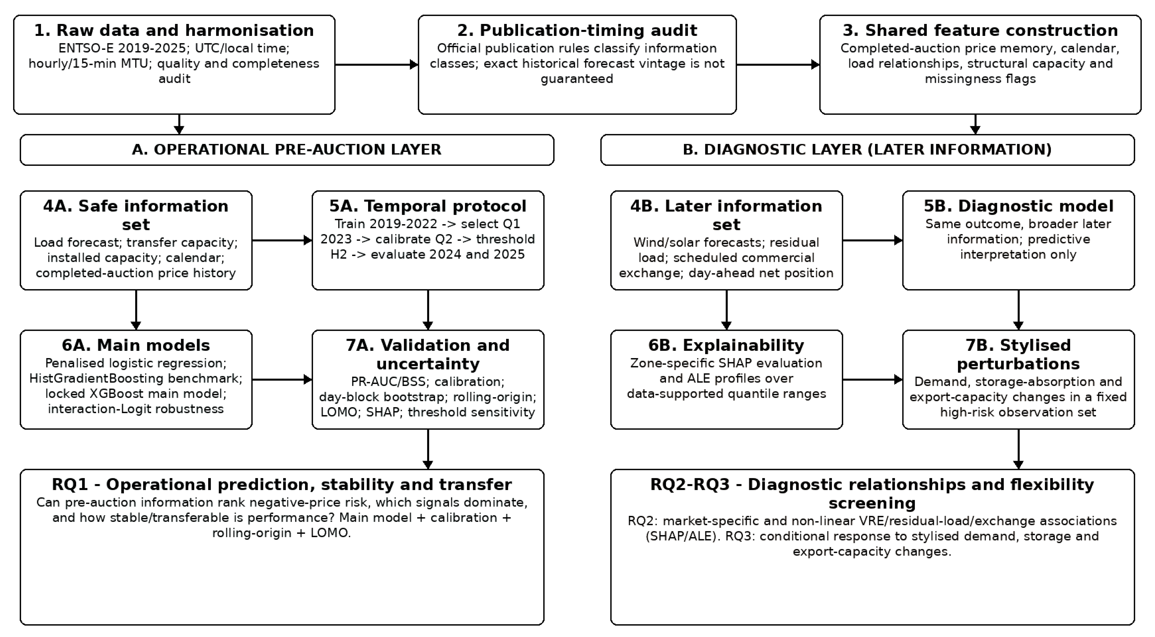Figure 1 presents the full workflow.

The analysis covered AT, BE, CH, CZ, DE_LU, DK1, DK2, FR, HR, IE_SEM, SI and SK. These units are bidding zones and do not always correspond to countries. Selection was deliberate and based on the availability of a consistent price series and sufficient coverage of load forecasts and structural variables. Consequently, the findings apply to the 12 selected bidding zones and are not automatically representative of all European bidding zones. IE_SEM after 2020 did not satisfy the load-forecast completeness criterion for the main model, whereas the diagnostic VRE extension covered only zone-years with sufficient wind and solar component coverage.

Table 1. Twelve bidding zones selected for the main and diagnostic analyses.

Zone	Bidding Zone	TSO(s)	Period	Analytical Status
AT	Austria	APG	2019–2025	Main
BE	Belgium	Elia	2019–2025	Main
CH	Switzerland	Swissgrid	2019–2025	Main
CZ	Czechia	ČEPS	2019–2025	Main; VRE diagnostic limited
DE_LU	Germany–Luxembourg	50Hertz; Amprion; TenneT DE; TransnetBW; Creos	2019–2025	Main
DK1	Denmark West	Energinet	2019–2025	Main
DK2	Denmark East	Energinet	2019–2025	Main
FR	France	RTE	2019–2025	Main
HR	Croatia	HOPS	2019–2025	Main; diagnostic from 2021
IE_SEM	Ireland/Northern Ireland SEM	EirGrid; SONI	2019–2020	Main; later years descriptive
SI	Slovenia	ELES	2019–2025	Main; VRE diagnostic limited
SK	Slovakia	SEPS	2019–2025	Main

Note: The title explicitly refers to 12 bidding zones. Selection was based on data availability and is discussed as a limitation on external validity. TSO, transmission system operator; VRE, variable renewable energy.

presents the spatial scope and analytical status of each bidding zone.

2.2. Predictor Timing, Harmonisation and Quality Control

The audit used the official ENTSO-E publication semantics. The day-ahead total load forecast should be published no later than two hours before gate closure [57], and forecasted day-ahead transfer capacity should be published one hour before gate closure [58]. By contrast, the fixed day-ahead version of the wind and solar forecast is published by 18:00 on D-1 [59], whereas scheduled commercial exchanges and net positions are published after allocation [60,61,62]. Single Day-Ahead Coupling (SDAC) documentation also identifies clearing prices, matched trades, scheduled exchanges and net positions as outputs of the common algorithm [62].

On this basis, two analytical layers were defined. The main model includes the load forecast, forecasted transfer capacities, structural capacities, calendar features and price history from completed auctions. The diagnostic model additionally includes wind and solar forecasts, residual load, scheduled commercial exchanges and net positions. This separation prevents information published late or after clearing from being treated as available to an operational pre-auction forecast.

The forecast origin for delivery day D was set immediately before the joint day-ahead auction closed on D-1, interpreted according to the local market calendar in Central European Time/Central European Summer Time (CET/CEST). The main model included only information classes whose regulatory publication deadlines preceded this point. Scheduled commercial exchanges, net positions and the fixed wind and solar forecast version published later were not treated as operational pre-auction predictors. The audit concerns the information class and publication rule; because the API archive does not permit reconstruction of every historical forecast revision, the forecast-vintage risk described in the limitations remains.

Table 2. Predictor availability before and after the day-ahead market gate closure.

Variable Group	Tier	Publication Rule	Analytical Limitation
Day-ahead total load forecast	Main	Published no later than two hours before day-ahead gate closure	Forecast-vintage risk remains
Forecasted day-ahead transfer capacity	Main	Published one hour before spot-market gate closure	Optional and incomplete on some borders
Installed capacities	Main	Structural information known in advance	Missingness flags retained
Price lags of 24/48/168 h and completed previous-day summaries	Main	Prices from earlier completed auctions	Constructed by local market date; no same-auction hours
Wind/solar generation forecast [14.1.D]	Diagnostic	Fixed day-ahead version published at 18:00 on D-1	Not guaranteed prior to the common day-ahead auction
Scheduled commercial exchange	Diagnostic	Published after allocation	Post-clearing outcome
Day-ahead net position	Diagnostic	Output of implicit allocation; published after allocation	Post-clearing outcome

Note: Publication rules describe the class of information, not necessarily the exact vintage returned by a later API download. The main model is therefore gate-closure-audited, but the absence of a complete historical forecast-vintage archive remains a limitation. API, application programming interface; D-1, the day before delivery.

summarises the assignment of variable groups to the main and diagnostic layers.

Historical forecast vintages require additional clarification. The raw authenticated-download archive and its download log record retrieval times, query labels and paths, and file hashes, while the stored forecast series are indexed by delivery time; they do not contain a complete per-observation publication or revision timestamp. Consequently, the retrievable archive cannot prove that every stored forecast observation is exactly the last version visible immediately before gate closure. The timing audit therefore applies to the official publication rule of the information class, not to a verified historical vintage of each observation. In this sense, “gate-closure-audited” means publication-rule-audited and leakage-controlled by information class; it does not mean perfectly vintage-clean. This limitation is carried explicitly into the interpretation of operational performance.

The full dataset contained 736,416 rows and 736,217 valid prices. Coordinated Universal Time (UTC) was the primary time axis, whereas local time was used to construct the market date, hour-of-day, calendar features and completed market days. An empty API response was treated as missing rather than zero. Neither prices nor targets were imputed. The data were stored in 12 partitions while retaining the source MTU and the number of sub-periods.

Zone-year combinations with at least 95% load-forecast completeness were included in the main model. This criterion was satisfied by 79 of 84 combinations; IE_SEM in 2021–2025 was excluded. After requiring a valid target, a load forecast and at least 168 h of price history, the main-model sample comprised 689,591 observations. The diagnostic model additionally required VRE components and was estimated on 531,822 observations from nine bidding zones with sufficient completeness.

Table 3. Data attrition from the harmonised panel to the main and diagnostic samples.

Dataset Component	N	Definition
Full harmonised panel	736,416	12 zones, 2019–2025
Valid day-ahead prices	736,217	Price and target not imputed
Negative periods	13,194	1.792%
Episodes of negative prices	2917	Consecutive within zone
Main-model sample	689,591	79 eligible zone-years
Diagnostic extension	531,822	9 zones with sufficient VRE/post-clearing data

presents the successive stages of sample reduction.

2.3. Target Definition, Episodes and Feature Engineering

The target NEG_PRICE took the value 1 when the day-ahead price in a given zone and period was strictly less than 0 EUR/MWh. A price equal to zero was classified as non-negative. Formally:

$$Y_{\mathrm{z},\mathrm{t}}=\mathbb{1}({P^{\mathrm{DA}}}_{\mathrm{z},\mathrm{t}}<0)$$

(1)

An episode was defined as an uninterrupted sequence of negative-price periods within the same bidding zone, ordered by TIMESTAMP_UTC. Following the SDAC transition to a 15 min MTU, from the delivery date of 1 October 2025, the base hourly price was calculated as the arithmetic mean of the available sub-period prices. Missing 15 min values were not imputed, and their number was retained in PRICE_SUBPERIOD_N. Two additional targets were used: NEG_ANY_SUBPERIOD indicated at least one negative quarter-hour within an hour, whereas NEG_ALL_SUBPERIOD indicated that all available quarter-hours were negative. The date 30 September 2025 refers to implementation and the relevant auctions, whereas 1 October 2025 was the first delivery day under the new MTU.

The main dataset comprised 48 columns. These included the level, 1, 3 and 6 h ramps, and rolling minima and maxima of the load forecast; forecasted import and export capacities; installed solar, onshore-wind, offshore-wind, pumped-storage and reservoir-hydro capacities; capacity-to-load ratios; hour-of-day, month and weekend features; missingness flags; and bidding-zone indicators.

The price history was constructed using 24, 48 and 168 h lags, as well as the minimum, mean, standard deviation and number of negative hours from the previous completed market day. In addition, the number of events and the average volatility over the past seven completed days were calculated. UTC served as the reference time: hourly lags denote the exact elapsed time in UTC, whilst daily summaries were grouped by LOCAL_DATE and therefore cover 23 or 25 periods on days when the clocks change. The summaries for the previous trading day do not include prices from the auction on the forecast day; the fixed hourly lags should be interpreted as measures of short-term price memory, with slight marginal ambiguity regarding local time during daylight saving time (DST) transitions.

P^lag(k)_z,t = P^DA_z,t−k,    k ∈ {24, 48, 168}

(2)

The diagnostic extension added wind and solar forecasts, the aggregate VRE forecast, forecast residual load, VRE share, residual-load share, residual-load ramps and rolling characteristics, as well as post-clearing scheduled commercial exchanges and net positions. These features were used for RQ2 and RQ3 but were not presented as an operational dataset available before gate closure.

2.4. Temporal Design, Models and Leakage Control

Training covered 2019–2022. Three distinct windows were used in 2023: the first quarter (Q1) for algorithm selection, the second quarter (Q2) for isotonic calibration and the second half of the year (H2) for selecting the threshold that maximised F1. The 2024 test and 2025 external test were not used to fit or tune the final pipeline. The final specification was refined following an audit of data quality and predictor availability; consequently, 2024–2025 are treated as chronological evaluation periods for the final procedure rather than as project-wide preregistered holdouts. The risks associated with this sequence were mitigated through an explicit protocol, locked hyperparameters and rolling-origin backtesting for 2020–2024.

Table 4. Time-separated model development and evaluation protocol.

Stage	Period	Roles
Training	2019–2022	Model estimation
Selection	Q1 2023	Compare logistic regression, HistGradientBoosting and XGBoost
Calibration	Q2 2023	Fit isotonic calibrator
Threshold	2023 H2	Choose the threshold that maximises F1
Test	2024	Primary evaluation after locked reconstruction
External test	2025	Temporal transfer and MTU assessment

Note: Q1, first quarter; Q2, second quarter; H2, second half of the year; XGBoost, Extreme Gradient Boosting.

summarises the role of each period.

Penalised logistic regression estimated by stochastic gradient descent (SGD), HistGradientBoosting and XGBoost were compared. The linear model used standardisation and class_weight = ‘balanced’. HistGradientBoosting used 250 iterations, a learning rate of 0.06, 15 leaves and L2 = 2. XGBoost used 350 trees, max_depth = 3, learning_rate = 0.05, min_child_weight = 6, subsample = 0.8, colsample_bytree = 0.8, reg_alpha = 0.1, reg_lambda = 2.5, scale_pos_weight = 10.5, tree_method = ‘hist’ and random seed 20260731. Hyperparameters were determined using only the training set and the Q1 2023 selection window and were not changed after evaluation in 2024–2025 began. The scale_pos_weight value of 10.5 formed part of the locked model specification.

XGBoost achieved the highest PR-AUC on the selection set and was selected as the main model. The isotonic calibrator was fitted exclusively on Q2 2023. A threshold of 0.042918 was selected by maximising F1 on H2 2023. This threshold is neither universal nor economically optimal; implementation requires a user-specific cost function.

The role of the benchmark models is deliberately different from coefficient-based econometric inference. The penalised logistic model provides a transparent low-complexity out-of-sample comparator on the same selection window, whereas XGBoost is used because the forecasting problem contains non-linearities, interactions, missingness patterns and heterogeneous market regimes. We do not interpret XGBoost feature attributions as structural parameters. The gain from the more flexible specification is therefore assessed by out-of-sample ranking and probability metrics rather than by statistical significance of individual coefficients.

To examine whether the XGBoost advantage could be reproduced by a lower-complexity functional form, an additional reviewer-requested robustness benchmark was estimated after the main pipeline had been locked. The benchmark used the same 2019–2022 training sample, standardisation, balanced class weighting and Q1 2023 out-of-sample selection window as the original penalised logistic comparator, but added six fixed, theory-motivated two-way interactions: VRE capacity-to-load × weekend, VRE capacity-to-load × hour cosine, VRE capacity-to-load × pumped-storage capacity-to-load, VRE capacity-to-load × forecasted export capacity, previous-day minimum price × previous-seven-day negative-period count, and previous-day minimum price × the 24 h price lag. The interactions were specified before evaluating this additional benchmark and were not used to retune XGBoost. For comparability beyond the selection window, the interaction model was passed through the same Q2 2023 isotonic-calibration and H2 2023 threshold-selection sequence before evaluation in 2024–2025.

The analysis was performed in Python 3.13.5 using NumPy 2.3.5, pandas 2.2.3, SciPy 1.17.0, scikit-learn 1.8.0, XGBoost 3.1.3, SHAP 0.50.0, joblib 1.5.3 and Matplotlib 3.10.8. The software environment is fully specified above.

2.5. Performance Evaluation, Calibration and Uncertainty

The main performance metric was PR-AUC, supplemented by ROC-AUC, precision, recall, F1, Brier score, log loss and the confusion matrix. Climatology, defined as a constant forecast equal to event prevalence in each evaluation set, served as the probabilistic benchmark for the Brier skill score (BSS). It was used as a retrospective reference for probabilistic skill rather than as a forecasting rule that could be implemented directly in real time. Penalised logistic regression and HistGradientBoosting served as algorithmic benchmarks for rare-event ranking. For the performance metrics below, Y_i ∈ {0,1} denotes the observed binary negative-price outcome for observation i, corresponding to the target defined in Equation (1), and ${\hat{\mathrm{p}}}_{\mathrm{i}}$ denotes the predicted probability of Y_i = 1.

$$\mathrm{Brier}=(1/\mathrm{N})·{{\sum }_{\mathrm{i}=1}}^{\mathrm{N}}{({\hat{\mathrm{p}}}_{\mathrm{i}}-{\mathrm{Y}}_{\mathrm{i}})}^2$$

(3)

BSS = 1 − Brier_model/Brier_climatology

(4)

$$\mathrm{logit}\left[\mathrm{Pr}\right({\mathrm{Y}}_{\mathrm{i}}=1\left)\right]=\mathrm{\alpha }+\mathrm{\beta }·\mathrm{logit}\left({\hat{\mathrm{p}}}_{\mathrm{i}}\right)$$

(5)

Calibration was assessed in 10 quantile bins using the expected calibration error (ECE), calibration intercept and calibration slope. The intercept α and slope β were estimated using the logistic recalibration in Equation (5); ideal calibration corresponds to α = 0 and β = 1. A positive intercept indicates that the observed event rate was, on average, higher than predicted, whereas a slope below 1 indicates excessive dispersion or overly extreme probabilities. Uncertainty was estimated with a 200-replicate percentile day-block bootstrap using seed 20260731. Complete LOCAL_DATE blocks were resampled jointly across all bidding zones, preserving within-day hourly dependence and contemporaneous conditions across zones; the procedure does not reproduce the full dependence between consecutive days.

In the episodic assessment, an episode was considered detected when at least one period within the observed sequence of negative prices exceeded a fixed probability threshold. False-positive zone-hours per calendar day were calculated as the total number of non-negative periods classified as positive across all zones, divided by the number of unique LOCAL_DATE values in a given evaluation set. The metric is aggregated across the entire panel and does not represent the average number of false-positive hours in a single zone.

A threshold-sensitivity check was performed on the locked calibrated XGBoost probabilities by multiplying the selected F1 threshold (0.042918) by 0.50, 0.75, 1.00, 1.25 and 1.50. No model parameters or predicted probabilities were refitted. For each operating point, precision, recall, F1, episode recall and false-positive zone-hours per day were recomputed separately for 2024 and 2025. This check isolates operating-point sensitivity from model-specification sensitivity.

2.6. Explainability, Transferability and Diagnostic Scenarios

SHAP values were calculated for the raw XGBoost models before calibration. Global feature importance was calculated as the mean absolute SHAP value. Zone-specific SHAP values for the diagnostic model were obtained by evaluating the same global model separately on observations from each bidding zone; separate zone-specific models were not fitted. The most important physical and post-clearing features were reported, with SHAP describing model behaviour rather than causal effects.

The non-linear component of RQ2 was assessed using Accumulated Local Effects (ALE) rather than one-dimensional partial dependence plots (PDPs). ALE was calculated for the same global diagnostic model over the observed evaluation-sample distribution, using 20 quantile intervals and local prediction differences. This approach reduced the creation of unrealistic combinations of correlated VRE-share and residual-load-share values. The profiles describe predictions from the diagnostic model rather than technical system thresholds.

LOMO was performed for the main model by excluding one bidding zone entirely from training, fitting the preprocessing and model on the remaining zones and evaluating performance in 2024. All bidding-zone dummy indicators were set to zero for the unseen zone; the experiment therefore measured transfer of common relationships. The reported zero-shot variant used a global calibrator fitted without data from the excluded zone; local-calibration results are provided in Supplementary File S1. IE_SEM did not satisfy the main-model completeness criterion after 2020, so the LOMO experiment covered 11 rather than 12 bidding zones.

Rolling-origin evaluation sequentially trained the fixed specification on data up to year y−1 and assessed the raw ranking in year y for 2020–2024. The scenarios were applied only to the diagnostic extension within the baseline highest-risk decile. The observation set was selected before perturbation and remained unchanged across all variants. Changes in load were accompanied by consistent recalculation of residual load and the associated shares; the storage-absorption proxy reduced residual surplus, and the combined variant applied both transformations. The numerical scenario outputs are reported in Supplementary File S1, but the calculations do not incorporate market equilibrium, costs, storage state of charge or responses in neighbouring bidding zones.

Figure 1 maps each analytical component to the information layer, the temporal window and the research question it addresses. The left branch contains the operational pre-auction workflow, including benchmark comparison, calibration, uncertainty assessment, rolling-origin validation and LOMO. The right branch contains the later-information diagnostic workflow, including SHAP/ALE interpretation and stylised perturbations. This separation is maintained throughout the Results and Discussion.

3. Results

3.1. Negative Prices Increased After 2022 but Remained Uneven Across Bidding Zones

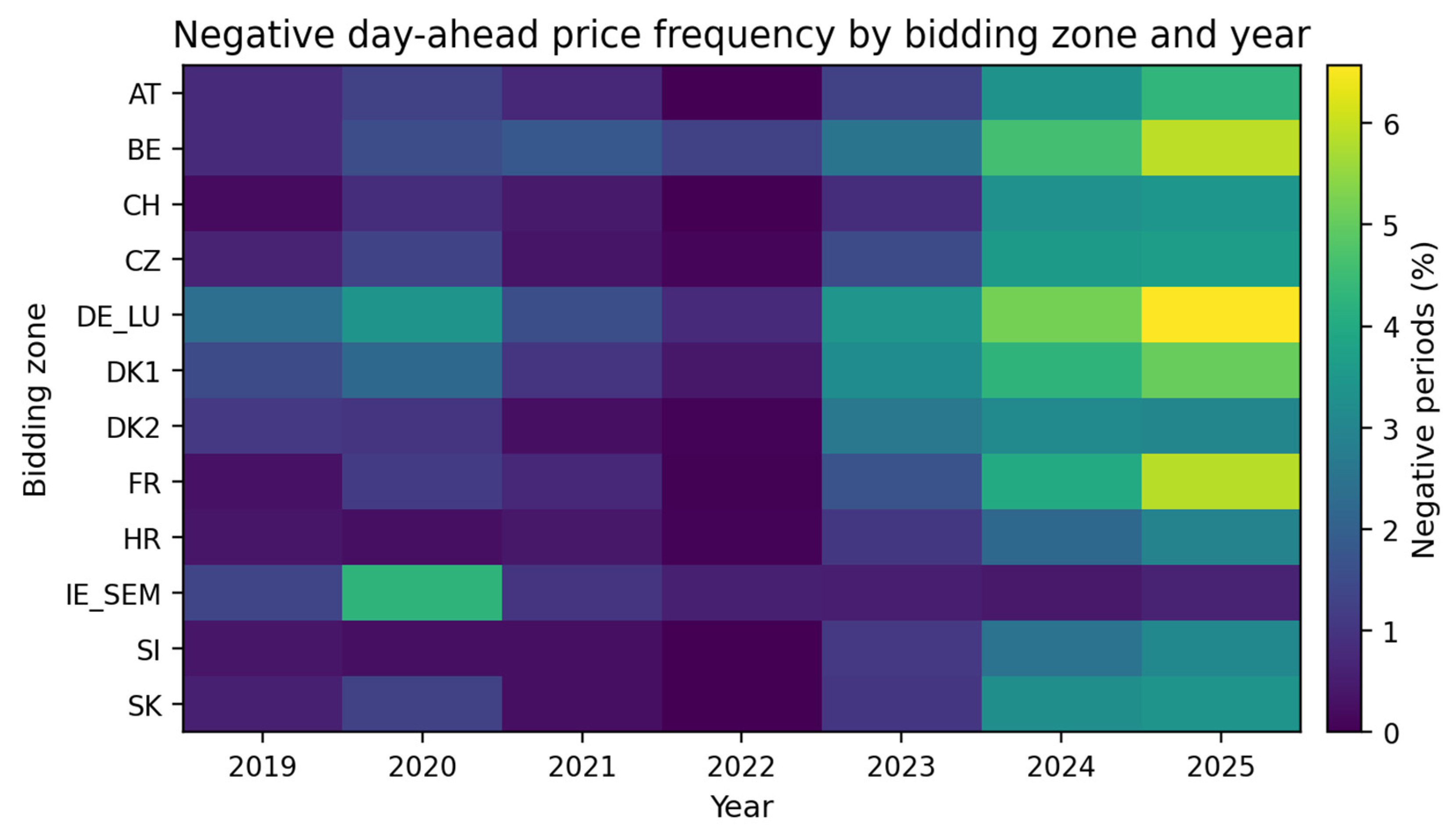
Among 736,217 valid observations, 13,194 negative-price periods (1.792%) and 2917 episodes were identified. The mean price was 101.10 EUR/MWh, the median was 77.23 EUR/MWh, the minimum was −500.00 EUR/MWh, and the maximum was 2987.78 EUR/MWh. The highest negative-price shares over the full period occurred in DE_LU (3.341%), BE (2.645%) and DK1 (2.519%), whereas the lowest occurred in HR (1.053%) and SI (1.082%).

Table 5. Negative-price exposure differed markedly across the 12 bidding zones.

Zone	Valid Observations	Negative Periods	Negative Share (%)	Episodes
AT	61,362	1028	1.675	239
BE	61,362	1623	2.645	379
CH	61,361	805	1.312	194
CZ	61,362	989	1.612	225
DE_LU	61,362	2050	3.341	392
DK1	61,362	1546	2.519	332
DK2	61,362	984	1.604	205
FR	61,362	1209	1.970	270
HR	61,362	646	1.053	170
IE_SEM	61,236	781	1.275	139
SI	61,362	664	1.082	162
SK	61,362	869	1.416	210

summarises bidding-zone differences,

Table 6. The frequency of negative prices accelerated after 2022.

Year	Valid Observations	Negative Periods	Negative Share (%)
2019	105,083	921	0.876
2020	105,371	1657	1.573
2021	105,083	785	0.747
2022	105,083	294	0.280
2023	105,083	1831	1.742
2024	105,396	3507	3.327
2025	105,118	4199	3.995

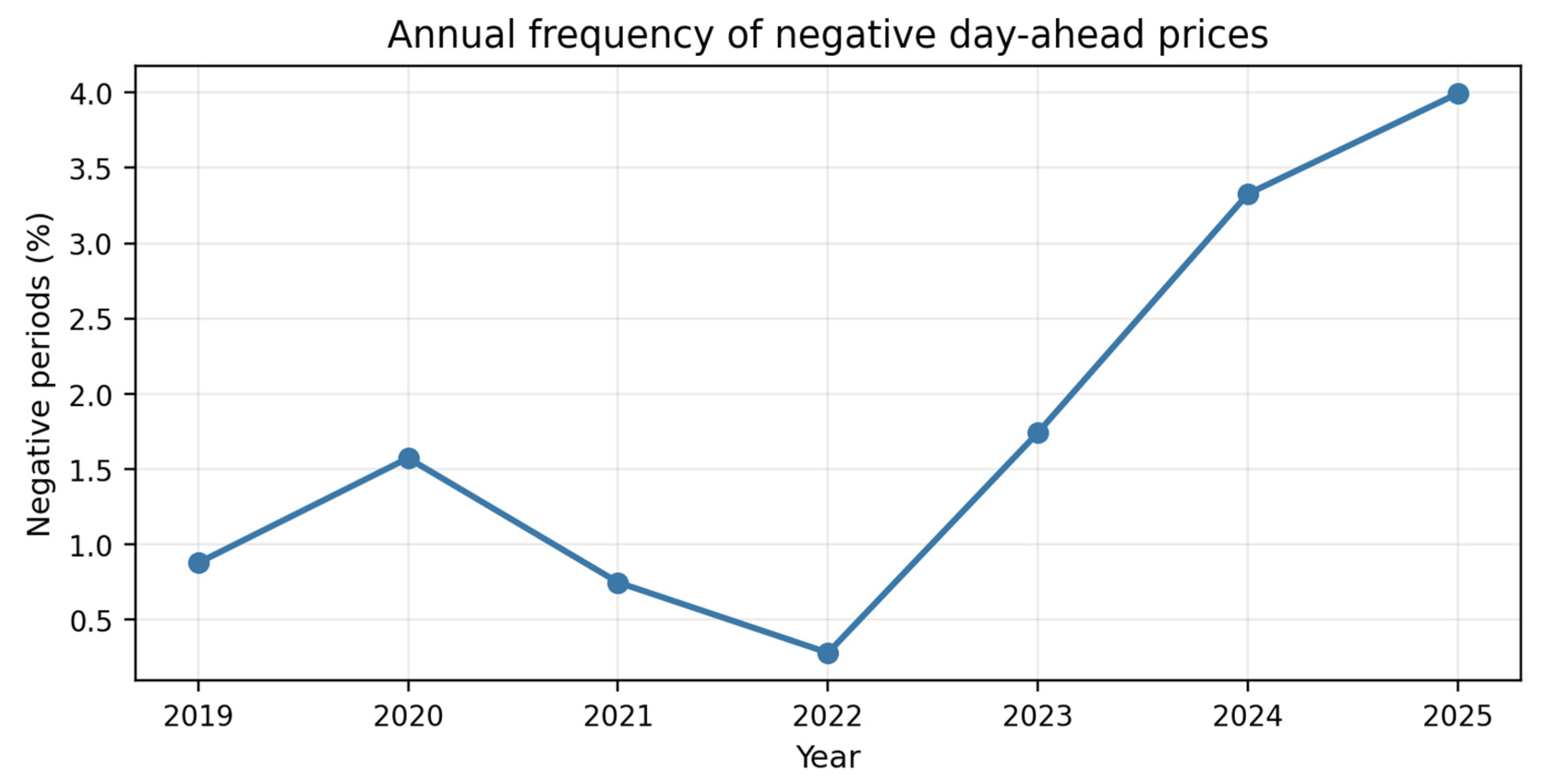
reports annual changes, and Figure 2 and Figure 3 illustrate their evolution.

The annual share fell to 0.280% in 2022 and then rose to 1.742% in 2023, 3.327% in 2024 and 3.995% in 2025. The increase was widespread but heterogeneous, supporting the inclusion of bidding-zone effects and separate transfer tests.

3.2. The Gate-Closure-Audited Model Achieved Moderate and Calibrated Predictive Skill

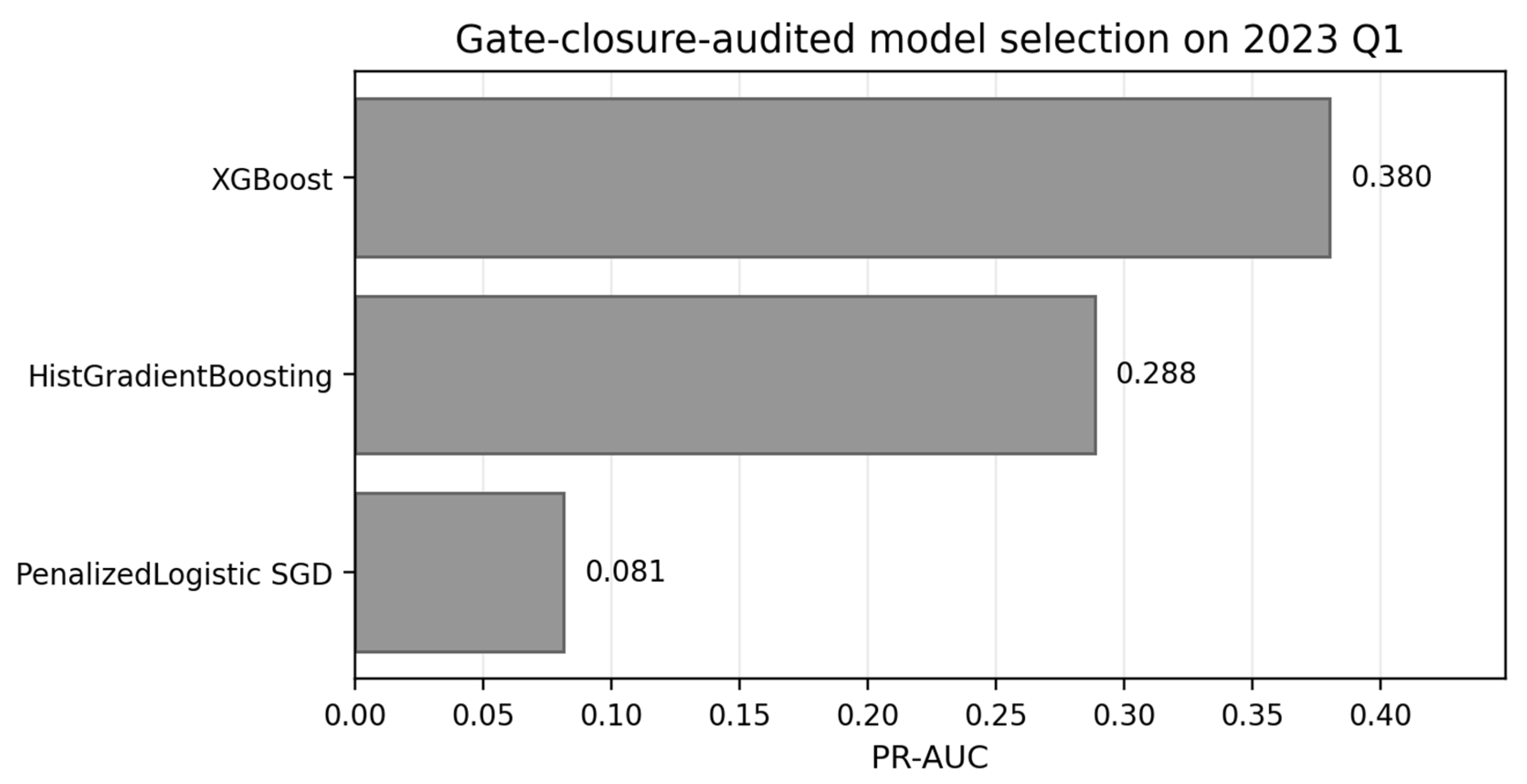
In the Q1 2023 selection window, XGBoost achieved a PR-AUC of 0.380, compared with 0.288 for HistGradientBoosting and 0.081 for penalised logistic regression. After the XGBoost architecture was locked, the isotonic calibrator was fitted on Q2 and the threshold selected on H2, the 2024 test yielded a PR-AUC of 0.409, a ROC-AUC of 0.923, precision of 0.295, recall of 0.639, F1 of 0.404 and a Brier score of 0.0267. A BSS of 0.227 indicated improvement over the climatology benchmark.

In the 2025 external test, PR-AUC was 0.436, precision was 0.406 and F1 was 0.489; recall was 0.616, the Brier score was 0.0328, and BSS was 0.203. The higher Brier score partly reflected higher event prevalence. The day-block bootstrap yielded a 95% confidence interval (CI) for PR-AUC of 0.320–0.502 in 2024 and 0.341–0.532 in 2025.

Table 7. Extreme Gradient Boosting (XGBoost) provided the strongest rare-event ranking on the 2023 selection window.

Model	PR-AUC	ROC-AUC	Precision	Recall	F1
Penalised logistic regression	0.081	0.946	0.024	0.967	0.046
HistGradientBoosting	0.288	0.980	0.085	0.942	0.156
XGBoost	0.380	0.979	0.252	0.725	0.374

Note: PR-AUC, area under the precision–recall curve; ROC-AUC, area under the receiver operating characteristic curve; XGBoost, Extreme Gradient Boosting.

and Figure 4 compare the algorithms, whereas

Table 8. The calibrated pre-auction model retained positive predictive ability in 2024 and 2025.

Split	N	Positive N	Prevalence	PR-AUC	ROC-AUC	Precision	Recall	F1	Brier	Brier Skill
2024 test	96,361	3449	0.036	0.409	0.923	0.295	0.639	0.404	0.027	0.227
2025 external	96,107	4134	0.043	0.436	0.935	0.406	0.616	0.489	0.033	0.203

Note: PR-AUC, area under the precision–recall curve; ROC-AUC, area under the receiver operating characteristic curve.

summarises the calibrated model’s 2024–2025 performance.

Because a random ranking has an expected PR-AUC equal to event prevalence, the absolute PR-AUC values should be read relative to the rarity of the target. In 2024, PR-AUC 0.409 was approximately 11.4 times the 3.58% event prevalence; in 2025, PR-AUC 0.436 was approximately 10.1 times the 4.30% prevalence. The term “moderate” therefore describes the absolute discrimination level and is not intended to imply an absence of useful skill; the positive BSS and episode-detection results provide complementary evidence.

The additional interaction-augmented penalised logistic benchmark did not close the performance gap. In Q1 2023 it achieved a PR-AUC of 0.060 and F1 of 0.055, compared with 0.081 and 0.046 for the original penalised logistic model and 0.380 and 0.374 for XGBoost. After the same calibration and threshold-selection sequence, its PR-AUC was 0.104 in 2024 and 0.132 in 2025, compared with 0.409 and 0.436 for XGBoost. The modest F1 improvement relative to the plain logistic model on the selection window therefore did not translate into comparable rare-event ranking, supporting the use of a non-linear tree model for this dataset while leaving causal interpretation outside the scope of the analysis.

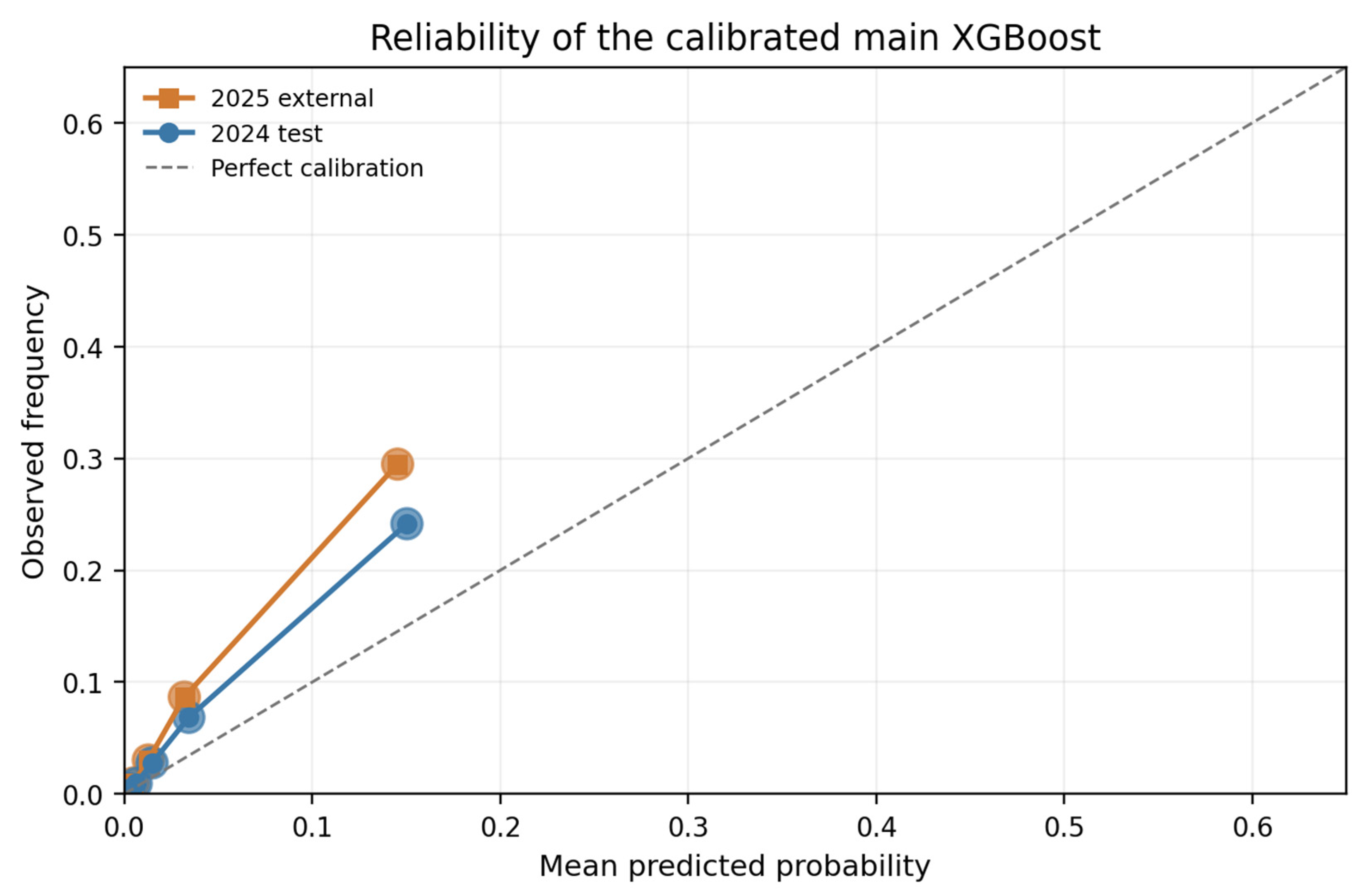
The quantile-based ECE was 0.0148 in 2024 and 0.0231 in 2025. Calibration slopes were close to 1 (0.911 and 0.967), whereas positive intercepts (0.527 and 1.053) indicated a shift in the baseline event rate and the need for periodic recalibration. The reliability diagram shows that most observations were concentrated in low-probability bins; therefore, a low ECE alone cannot replace analysis of the highest-risk deciles. In the highest-risk quantile bin, the mean predicted probability and observed frequency were 0.150 and 0.242 in 2024, respectively, and 0.145 and 0.295 in 2025, making the upward shift in the baseline event rate particularly visible.

At the fixed threshold, the model detected 486 of 742 episodes in 2024 (65.5%) and 559 of 895 episodes in 2025 (62.5%). False-positive zone-hours per calendar day, aggregated across the entire panel, were 14.38 and 10.20, respectively; these values do not represent a single bidding zone. The model is useful as a ranking and screening layer, but the operating threshold must be chosen locally using application-specific alarm costs.

Table 9. Calibration drift coexisted with stable episode detection across 2024 and 2025.

Split	ECE (10 Quantile Bins)	Calibration Intercept	Calibration Slope	Episode Recall	FP Zone-Hours/Day
2024 test	0.0148	0.527	0.911	0.655	14.38
2025 external	0.0231	1.053	0.967	0.625	10.20

Note: ECE, expected calibration error; FP, false positive; FP zone-hours/day, false-positive zone-hours per calendar day aggregated across all bidding zones in the evaluation sample.

reports detailed calibration and episode-detection metrics, and Figure 5 shows the relationship between predicted and observed frequencies.

Threshold sensitivity confirmed the expected precision–recall trade-off without changing the ranking model. In 2024, halving the threshold from 0.042918 to 0.021459 increased period recall from 0.639 to 0.878 and episode recall from 0.655 to 0.883, but reduced precision from 0.295 to 0.150 and increased false-positive zone-hours per day from 14.38 to 47.03. Raising the threshold by 50% to 0.064378 increased precision to 0.517 and reduced false positives to 3.65 per day, while period recall fell to 0.415 and episode recall to 0.472. The same directional pattern occurred in 2025: at 0.021459, period and episode recall were 0.882 and 0.895 with 41.58 false-positive zone-hours per day, whereas at 0.064378 they were 0.397 and 0.440 with 2.85 false positives per day. The substantive conclusion is therefore stable—the model provides a useful screening ranking—but the operational trade-off depends strongly on the local alarm cost.

3.3. Predictive Performance Shifted Across Years and Following the 15 min MTU Transition

The rolling-origin PR-AUC was 0.147 in 2020, 0.176 in 2021, 0.095 in 2022, 0.307 in 2023 and 0.495 in 2024. The result of 0.495 for 2024 is not directly comparable with the baseline test result of 0.409: in the rolling-origin approach, the fixed specification was retrained on data up to the end of 2023 and the raw ranking was evaluated, whereas the main protocol used the years 2019–2022 for estimation, and 2023 solely for selection, calibration and threshold setting. Variability between years reflects both changes in prevalence and domain shift; high performance in years with more frequent events should not be directly extrapolated to regimes with very low incidence.

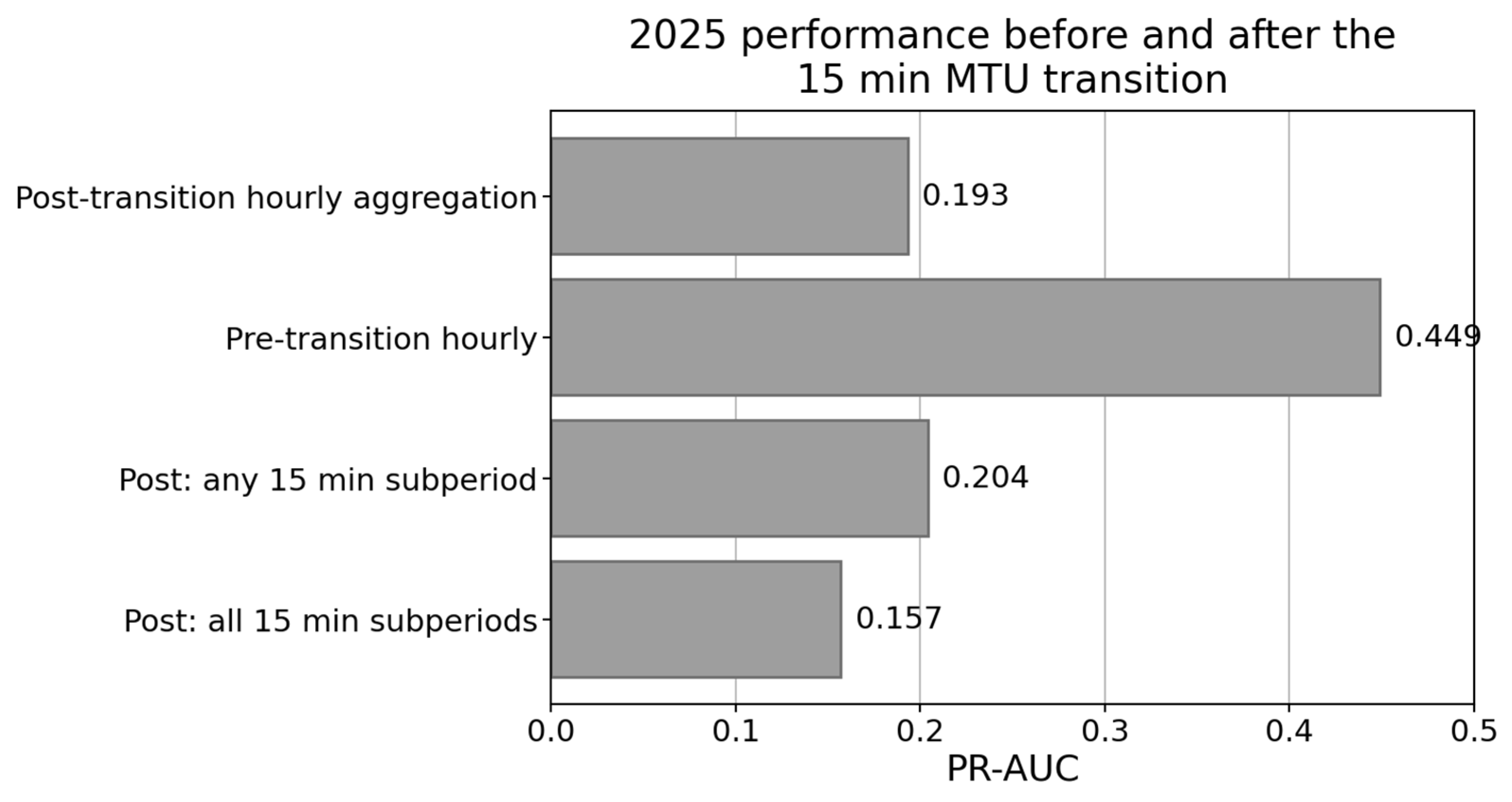
In 2025, before the MTU transition, the model achieved a PR-AUC of 0.449 at an event prevalence of 5.53%. After 1 October, when prevalence fell to 0.66%, the PR-AUC was 0.193. Under the ANY and ALL definitions, the PR-AUC was 0.204 and 0.157, respectively. The post-transition results are based on a shorter period and fewer events; they therefore do not isolate an independent MTU effect but demonstrate the need for a native 15 min model.

Table 10. Predictive ranking varied substantially across annual market regimes.

Train Through	Test Year	Test N	Positive N	Prevalence	PR-AUC	ROC-AUC
2019	2020	105,213	1641	0.016	0.147	0.889
2020	2021	96,338	696	0.007	0.176	0.909
2021	2022	96,290	243	0.003	0.095	0.954
2022	2023	96,265	1783	0.019	0.307	0.928
2023	2024	96,361	3449	0.036	0.495	0.941

Note: PR-AUC, area under the precision–recall curve; ROC-AUC, area under the receiver operating characteristic curve.

reports the rolling-origin results, whereas

Table 11. Predictive performance before and after the transition to a 15 min market time unit.

2025 Period/Target	N	Positive N	Prevalence	PR-AUC	Brier Skill
Post-transition hourly mean	24,201	160	0.007	0.193	0.098
Pre-transition hourly	71,906	3974	0.055	0.449	0.198
Post: any negative 15 min sub-period	24,201	209	0.009	0.204	0.097
Post: all negative 15 min sub-periods	24,201	118	0.005	0.157	0.059

Note: PR-AUC, area under the precision–recall curve.

and Figure 6 compare performance before and after the MTU transition.

3.4. Auction-Aligned Price Memory Dominated the Pre-Auction Risk Signal

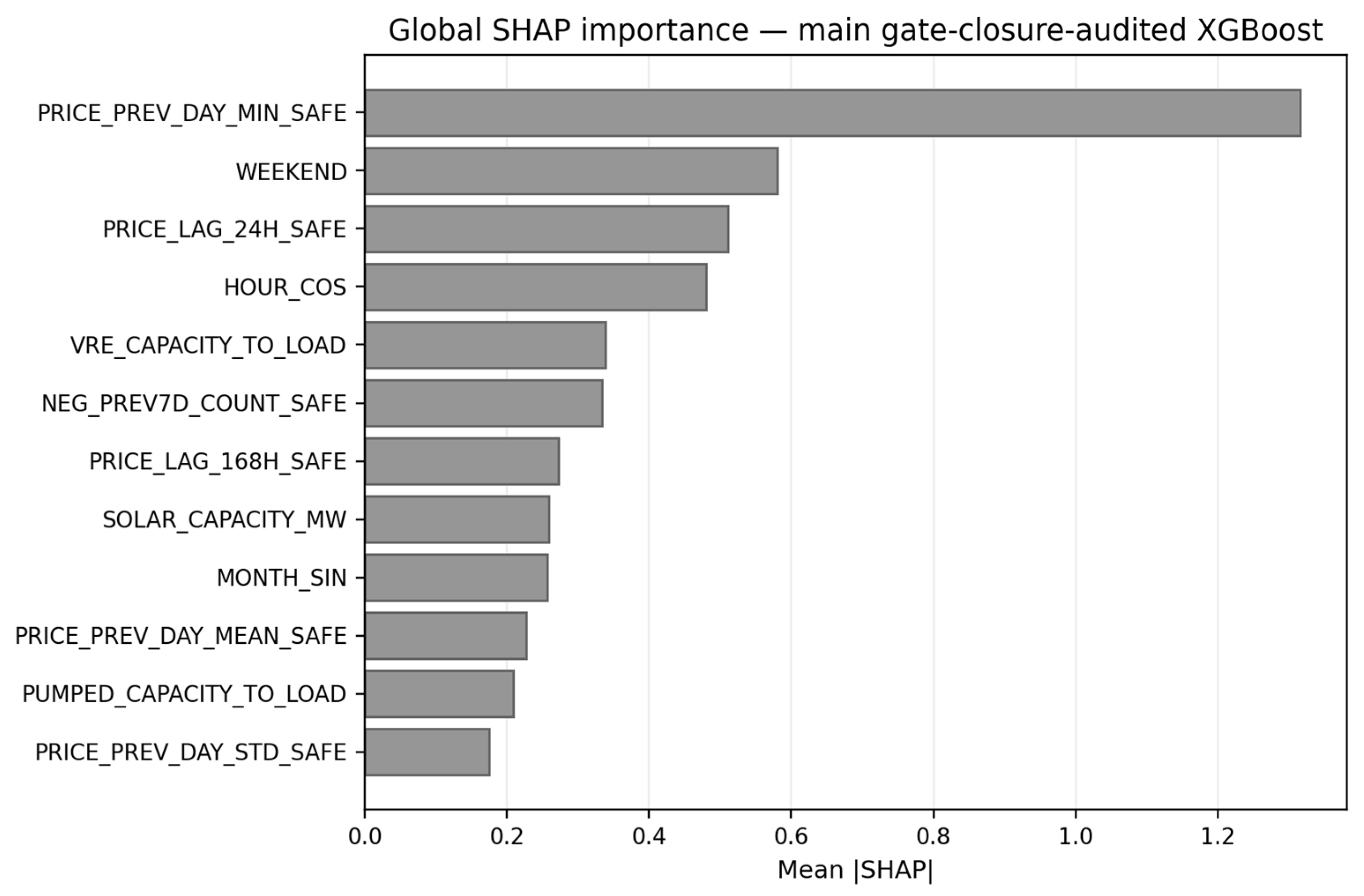
The strongest feature of the main model was the minimum price of the previous completed market day (mean |SHAP| = 1.316). This was followed by the weekend (0.580), the 24 h safe lag (0.511), HOUR_COS (0.480), the ratio of installed VRE capacity to the load forecast (0.338), the number of negative hours in the previous seven days (0.334) and the 168 h lag (0.272).

The dominance of auction-aligned price memory does not constitute data leakage because the prices originate from completed auctions. It nevertheless shows that information on the current market regime is stronger than any single structural indicator. Calendar features and capacity-to-load ratios act as carriers of recurring configurations rather than autonomous causes.

Table 12. Recent negative-price history and calendar effects dominated the pre-auction risk signal.

Predictor	Mean |SHAP|
PRICE_PREV_DAY_MIN_SAFE	1.316
WEEKEND	0.580
PRICE_LAG_24H_SAFE	0.511
HOUR_COS	0.480
VRE_CAPACITY_TO_LOAD	0.338
NEG_PREV7D_COUNT_SAFE	0.334
PRICE_LAG_168H_SAFE	0.272
SOLAR_CAPACITY_MW	0.259
MONTH_SIN	0.257
PRICE_PREV_DAY_MEAN_SAFE	0.227
PUMPED_CAPACITY_TO_LOAD	0.210
PRICE_PREV_DAY_STD_SAFE	0.175

Note: SHAP, SHapley Additive exPlanations.

and Figure 7 present the full feature ranking.

3.5. VRE, Residual Load and Cross-Border Flows Provided Market-Specific Diagnostic Information

The diagnostic extension, which includes VRE forecasts and post-clearing scheduled exchange and net-position data, achieved a PR-AUC of 0.464 and BSS of 0.272 in 2024, and a PR-AUC of 0.492 and BSS of 0.251 in 2025. It therefore showed stronger diagnostic discrimination than the main model but does not represent a pre-auction forecast; rather, it demonstrates the value of information that becomes available later in the market sequence.

Globally, the most important diagnostic features beyond safe price history were NET_SCHEDULED_IMPORT_MW (0.452), VRE_FORECAST_MW (0.423), RESIDUAL_LOAD_SHARE (0.380), VRE_SHARE_FORECAST (0.350), FORECAST_RESIDUAL_LOAD_MW (0.317) and RESIDUAL_ROLLING_MIN_6H (0.310). The zone-level pattern differed markedly: scheduled imports dominated in DK1 and DK2, residual load in FR and DE_LU, and VRE-related shares in BE, CH, HR and SK.

Table 13. Later, variable renewable energy (VRE) and market-coupling information improved diagnostic discrimination.

Split	N	Positive N	PR-AUC	ROC-AUC	Precision	Recall	F1	Brier Skill
2024 test	79,036	2933	0.464	0.953	0.476	0.544	0.508	0.272
2025 external	78,631	3551	0.492	0.952	0.538	0.476	0.505	0.251

Note: VRE, variable renewable energy; PR-AUC, area under the precision–recall curve; ROC-AUC, area under the receiver operating characteristic curve.

summarises overall diagnostic-model performance, and

Table 14. Dominant physical and cross-border signals differed by bidding zone.

Zone	Rank 1	Rank 2	Rank 3
AT	Scheduled net imports (0.462)	VRE forecast (0.337)	Residual-load share (0.331)
BE	Residual-load share (0.480)	VRE forecast (0.417)	VRE forecast share (0.400)
CH	VRE forecast (0.388)	Scheduled net imports (0.388)	VRE forecast share (0.355)
DE_LU	Forecast residual load (0.762)	6 h residual-load minimum (0.664)	VRE forecast (0.566)
DK1	Scheduled net imports (0.828)	Residual-load share (0.527)	VRE forecast share (0.443)
DK2	Scheduled net imports (0.806)	VRE forecast (0.489)	Residual-load share (0.445)
FR	Forecast residual load (0.996)	Scheduled net imports (0.693)	6 h minimum residual load (0.586)
HR	VRE forecast (0.401)	Scheduled net imports (0.291)	Residual-load share (0.272)
SK	VRE forecast (0.485)	VRE forecast share (0.389)	Residual-load share (0.375)

Note: Values are mean absolute SHAP contributions obtained by evaluating the same global diagnostic model separately for each bidding zone; separate zone-specific models were not fitted. The values are predictive attributions, not structural or causal effects. CZ and SI lacked complete wind components; IE_SEM lacked the required diagnostic sample. SHAP, SHapley Additive exPlanations; VRE, variable renewable energy.

reports the zone-level hierarchy of signals.

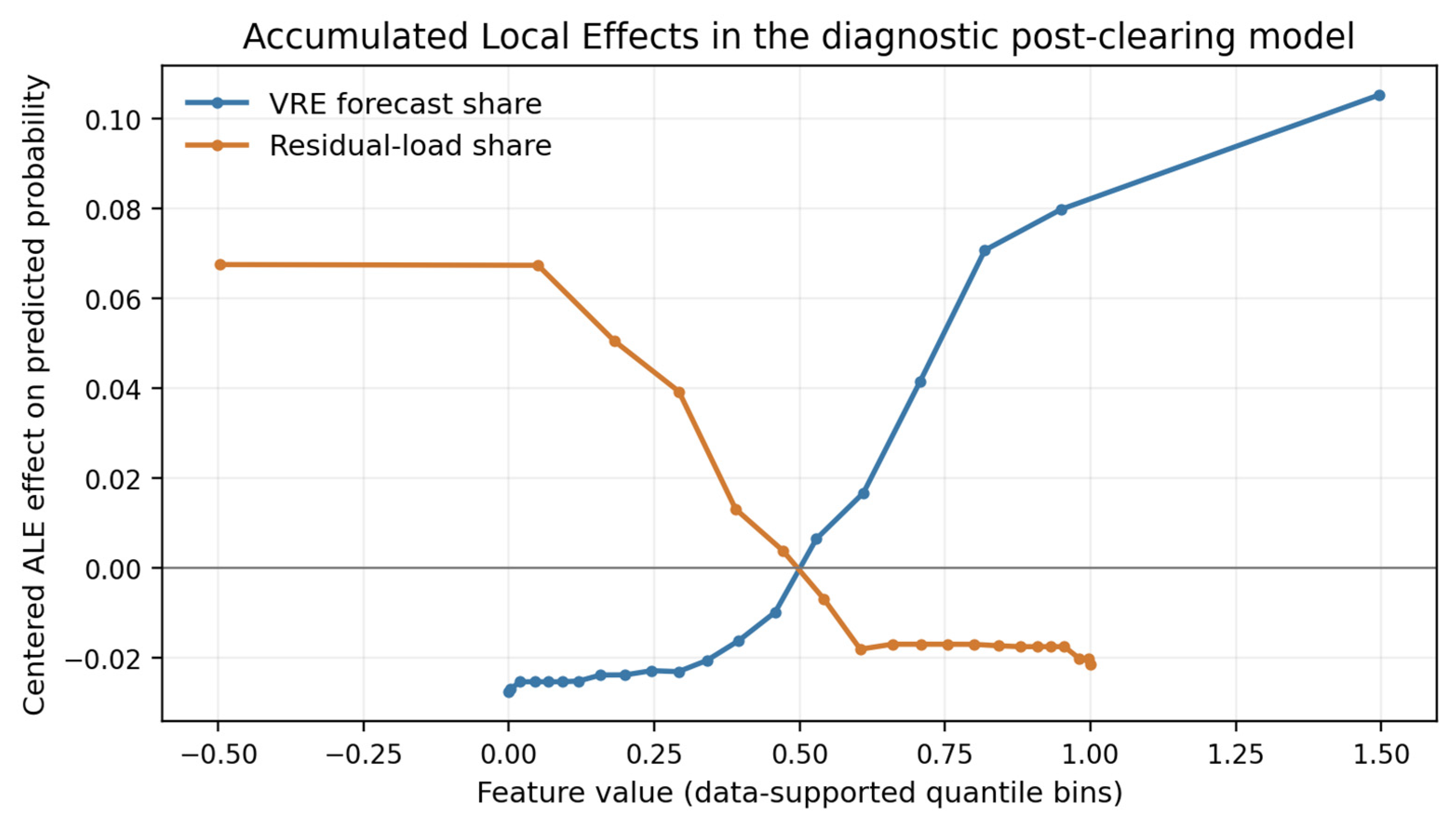
The ALE profile for VRE_SHARE_FORECAST remained negative or close to zero in the lower ranges and then increased markedly from approximately 0.49, particularly above 0.65. For RESIDUAL_LOAD_SHARE, the largest decline in ALE occurred between approximately 0.12 and 0.58. These are quantile-based, data-supported ranges of model response rather than universal technical thresholds.

The use of ALE mitigates the problem of unrealistic feature combinations typical of simple one-at-a-time profiles. However, the result remains dependent on the diagnostic model, which incorporates information published late or after clearing. The ALE profiles are shown in Figure 8.

Figure 8 should be read only as a model-response plot over the empirical support of the diagnostic sample. The ALE calculation uses 20 quantile intervals, and each interval contained 546 or 547 evaluation observations for each displayed feature. Consequently, wider intervals on the x-axis identify sparser portions of the predictor distribution even though the bin counts are nearly equal. The x-axis values are not engineering thresholds, and the figure is not evidence that a particular VRE or residual-load share has universal physical significance.

3.6. Cross-Zone Transfer Was Positive but Heterogeneous

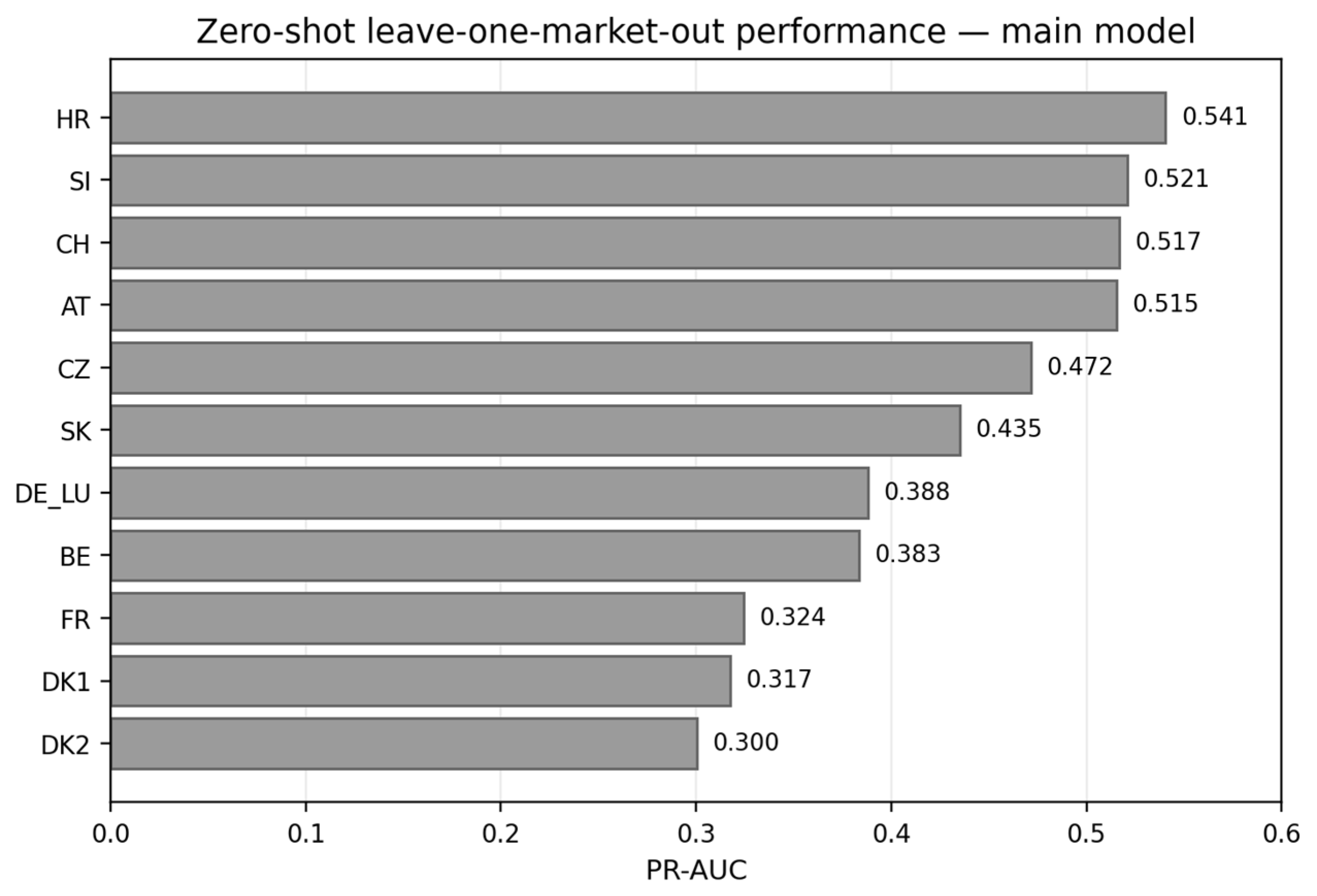
Zero-shot LOMO for the main model yielded PR-AUC values from 0.300 in DK2 to 0.541 in HR. The highest values were recorded in HR (0.541), SI (0.521), CH (0.517) and AT (0.515). PR lift ranged from 7.43 to 24.47. All 11 eligible bidding zones had positive Brier skill scores, ranging from 0.153 to 0.355, indicating better probabilistic performance than a constant forecast equal to local event prevalence, although local calibration remained necessary.

LOMO does not measure institutional similarity and, because all bidding-zone dummy indicators are zero for the held-out market, it excludes a learned zone-specific effect. The results indicate that some common relationships transfer across bidding zones, but the extent of transfer varies markedly; the PR-AUC differences therefore continue to support a global–local architecture.

Table 15. Cross-zone transfer remained useful but heterogeneous across held-out markets.

Held-Out Zone	N	Positive N	Prevalence	PR-AUC	PR Lift	Recall	Brier Skill
DK2	8782	275	0.031	0.300	9.585	0.709	0.153
DK1	8782	375	0.043	0.317	7.435	0.555	0.176
FR	8782	352	0.040	0.324	8.088	0.722	0.173
BE	8782	404	0.046	0.383	8.330	0.611	0.205
DE_LU	8781	457	0.052	0.388	7.458	0.654	0.193
SK	8782	288	0.033	0.435	13.261	0.483	0.174
CZ	8782	315	0.036	0.472	13.149	0.610	0.201
AT	8782	296	0.034	0.515	15.293	0.662	0.355
CH	8782	292	0.033	0.517	15.546	0.517	0.163
SI	8542	201	0.024	0.521	22.139	0.517	0.255
HR	8782	194	0.022	0.541	24.468	0.778	0.217

Note: IE_SEM was not included because it did not satisfy the main-model completeness criterion after 2020; therefore, 11 bidding zones were eligible for held-out-market evaluation. PR-AUC, area under the precision–recall curve; PR lift, PR-AUC divided by event prevalence.

reports the complete zone-level results, and Figure 9 provides a visual comparison.

3.7. Stylised Demand and Storage-Absorption Perturbations Were Associated with Lower Diagnostic-Model Risk

In the baseline top decile of diagnostic model risk (N = 8087), selected prior to the introduction of perturbations and kept unchanged across all variants, the mean prediction was 0.198. A consistent 5% and 10% increase in load reduced the average prediction by 1.906 and 3.714 percentage points, respectively. The proxy for additional storage absorption reduced it by 1.042 percentage points, whilst the combined variant reduced it by 2.802 percentage points. A 10% increase in export capacity alone resulted in a slight change of +0.102 percentage points.

The numerical outputs are reported in full in Supplementary File S1, but they do not constitute a counterfactual assessment of demand response, storage investment or interconnector policy. The positive sign of the isolated capacity perturbation shows that capacity alone, without changes in utilisation or conditions in neighbouring bidding zones, does not represent actual exports.

Table 16. Conditional diagnostic-model predictions under stylised demand, storage-absorption and export-capacity perturbations.

Scenario	Top-Decile N	Base Probability	Scenario Probability	Change (p.p.)	Base High-Risk	Scenario High-Risk
Demand +5%	8087	0.198	0.179	−1.906	3350	2950
Demand +10%	8087	0.198	0.161	−3.714	3350	2579
Storage-absorption proxy	8087	0.198	0.187	−1.042	3350	3150
Export capacity +10%	8087	0.198	0.199	0.102	3350	3361
Combined	8087	0.198	0.170	−2.802	3350	2759

Note: The complete scenario results are provided in Supplementary File S1. These results are non-causal and do not form part of the gate-closure evidence. p.p., percentage points.

reports the complete results of the stylised perturbations.

4. Discussion

4.1. Rising Negative-Price Frequency Is Consistent with Multiple Absorption Constraints, Not a Single Renewable Effect

The increase in negative-price frequency between 2023 and 2025 is consistent with European evidence of more hours with very low and negative prices as VRE shares increase [1,2,3,4,22]. This finding reinforces the importance of demand flexibility, storage, grid capacity and controllable resources in systems with high variable generation, in line with research on residual load, demand response, storage and the declining market value of VRE [11,12,13,14,15,16]. At the same time, the long-term development of renewable energy and changes in energy balances across EU Member States have been spatially heterogeneous, as shown by studies of renewable-energy deployment and the structure of energy production, consumption, imports and exports [63,64]. This does not establish that renewable-energy growth alone causes negative prices, because demand, fuel and emissions costs, hydrology, minimum-generation constraints, support schemes and bidding strategies also changed. Studies of the German market and multi-market analyses likewise support a multi-factor interpretation [6,7,8,9,10,17,18,19,20,21].

Differences between DE_LU, BE, DK1 and bidding zones with lower negative-price frequency confirm the importance of local technological and market configurations, consistent with literature showing heterogeneous effects of VRE, support mechanisms and market integration [19,20,21,22,23,24,25]. Heterogeneity is also present in the retail segment: a study of household electricity prices in the EU found substantial differences in price levels, dynamics and relationships with energy-system characteristics [65]. Although retail prices are not direct counterparts of day-ahead prices, this evidence reinforces the need for cautious cross-market comparison. A negative price remains a market-clearing outcome and may serve as an observable signal of hours in which the system and market have limited capacity to absorb surplus generation under existing bids and constraints. It is not, however, a direct measure of flexibility, curtailment or system security, because actual absorption also depends on storage, flexible demand, unit constraints and cross-border exchange capability [11,12,13,14,15,16,21].

4.2. Timing-Audited Information Produces More Credible but More Moderate Pre-Auction Performance

A credible interpretation of market-stress signals requires distinguishing a product label from its publication time. Load forecasts and forecasted transfer capacities are generally available before day-ahead gate closure [57,58]. Wind and solar forecasts published by 18:00 on D-1 are not guaranteed to be available before the joint auction, whereas scheduled exchanges and net positions are allocation outcomes [59,60,61,62]. Without this timing audit, apparently strong predictive performance may describe a later market stage rather than a genuine pre-auction forecast. This concern is consistent with broader recommendations on chronological validation, test-period protection and unambiguous forecast origin [29,30,31,32,33,50,51,52].

Separating the information layers preserves the credibility of the main conclusion. The pre-auction model achieved moderate PR-AUC values of 0.409–0.436 and positive Brier skill. The diagnostic extension incorporating VRE, residual load and market-coupling outcomes better describes the physical and spatial signals associated with negative-price periods but does not constitute an operational pre-clearing forecast. This distinction follows recommendations to assess accuracy, calibration, interpretability and generalisability as separate dimensions of model quality [26,27,28,41,42].

A forecast-vintage limitation remains: the API may return the most recently revised forecast rather than the historical version available immediately before gate closure. Full operational validation requires real-time archiving and reconstruction of the information available at each decision point, consistent with principles for sound evaluation of time-series forecasts [50,51,52,54,55,56]. We therefore use the term ‘gate-closure-audited’ rather than ‘perfect vintage-clean forecast’.

4.3. Operational Value Requires Calibration, Local Thresholds and Regime Monitoring

XGBoost outperformed the benchmark models on the selection set, but the tests show that ranking and probability estimation are distinct tasks. Positive BSS values in both years indicate that the calibrated model improved on the climatology benchmark; however, the calibration intercept and ECE reveal drift. This is consistent with literature showing that ranking metrics for rare events do not replace probability-calibration assessment [35,36,37,38,39,40]. The model should therefore be recalibrated periodically rather than deployed with one fixed threshold across multiple years, particularly as price regimes change [41,42].

Episode recall of approximately 63–65% is operationally informative, but the aggregate number of false-positive zone-hours across the panel remains high. This indicator is not the average number of false alarms in a single bidding zone. Transmission system operators (TSOs), aggregators and storage operators face different costs of false positives and false negatives. The threshold of 0.042918 was selected to maximise F1 and is only a research operating point; it cannot replace a cost-based decision rule, and its interpretation should account for the limitations of classification metrics under severe class imbalance [34,35,36,37,38].

Moderate absolute ranking performance should therefore not be interpreted as a failed forecast. For a target occurring in only about 3.6–4.3% of evaluation observations, PR-AUC was more than ten times the prevalence baseline in both years, while BSS remained positive. At the same time, this level of performance is not sufficient for autonomous control; it supports the paper’s narrower claim that the model is a screening layer whose probabilities and thresholds require local calibration.

The bootstrap intervals are wide and overlap between 2024 and 2025. The results therefore do not establish that the model improved in 2025; the point difference may reflect event prevalence and sample composition. Rolling-origin evaluation further shows that performance depends strongly on the annual regime, supporting multi-period out-of-sample assessment rather than reliance on a single data split [50,51,52].

The 2025 calibration shift is consistent with a changed European market environment rather than with one isolated technical cause. The IEA reports that average EU wholesale electricity prices increased by about 10% year on year in 2025, alongside roughly 9% higher TTF gas prices and higher EU-ETS prices, while negative-price hours became more frequent in several European markets [1]. The model diagnostics show the shift directly: in the highest-risk calibration bin, mean predicted probability versus observed frequency was 0.150 versus 0.242 in 2024 and 0.145 versus 0.295 in 2025. Such simultaneous changes in fuel costs, renewable-output patterns, demand and system availability can alter both the baseline event rate and the mapping from pre-auction features to negative-price probabilities. These external developments are therefore plausible contributors to the positive calibration intercept in 2025, but the present design does not identify their individual causal effects.

4.4. Physical and Cross-Border Predictive Signals Vary Across Markets

The main model is dominated by lagged price information and calendar features, demonstrating the importance of market-regime memory. This is consistent with price-forecasting literature, in which lagged prices and seasonal patterns are key information sources [27,28,29,30,31,32,33]. Physical conditions are nevertheless important. The diagnostic extension reveals the additional importance of VRE, residual load and cross-border exchange, broadening the interpretation of a negative price as a signal of the configuration of demand, supply and absorption capacity, in line with research on the merit-order effect, residual load and market integration [6,7,8,9,10,11,12,13,14,15,16,17,18,19,20,21]. Separating the information layers prevents economic interpretation from being conflated with the operational availability of predictors.

Zone-level SHAP values provide a numerical answer to RQ2: scheduled imports are especially important in DK1 and DK2, residual load in DE_LU and FR, and VRE-share features in several other bidding zones. This heterogeneity is consistent with studies reporting spatial effects of market integration and different profiles of renewable-energy impacts [17,21,25]. These differences are not causal structural properties of the markets; they may reflect data distributions, completeness, correlations and model architecture. SHAP values should therefore be interpreted as predictive attributions [45,46,49].

ALE addresses the non-linear component of RQ2 without generating highly unrealistic feature combinations. The increase in model response for VRE share above approximately 0.49 and the decrease associated with residual-load share in the middle ranges are consistent with surplus conditions but do not define universal technical thresholds. Interpretation must remain local and predictive, in accordance with the properties and limitations of ALE for correlated predictors [47,48].

LOMO for the main model produced positive BSS values in all 11 eligible bidding zones. At the same time, PR-AUC values of 0.300–0.541 indicate partial rather than complete transfer of common relationships across markets. This finding is consistent with transfer-learning literature, which links transfer performance to differences in distributions and institutional conditions [53]. A global model may provide a starting point, but final probabilities should be calibrated locally and monitored after changes in market design [41,42,50,51,52,53].

The transition to a 15 min MTU highlights the importance of market governance. The post-transition decline in PR-AUC coincided with substantially lower event prevalence and a short evaluation window, so it cannot be attributed solely to the MTU change [5]. Native quarter-hourly models should be developed, with episode duration, price depth and the operational value of alerts modelled separately. This follows the broader principle that forecasting methods should adapt to changes in market design and data resolution [26,27,28,41,42].

4.5. Flexibility Diagnostics Support Conditional, Not Causal, Implications

Consistently recalculated demand and storage-absorption scenarios point towards greater energy absorption and support the interpretation of flexibility. This is consistent with literature indicating that demand response, storage and temporal load shifting can mitigate VRE surpluses [11,12,13,14,15,16]. The scenarios do not, however, demonstrate policy effectiveness or investment profitability. The absence of state-of-charge dynamics, efficiency, costs, rebound effects, supply responses and inter-zonal market equilibrium prevents them from being treated as complete counterfactual scenarios.

For system and market operators, the main model can rank periods requiring further analysis; for aggregators and storage operators, it can serve as a screening layer before a local decision model. The diagnostic extension may support monitoring after additional VRE and market-coupling information becomes available. Investors should combine the signal with storage optimisation, forward curves, degradation costs and other markets, whereas regulators should treat a negative price as a symptom of market configuration rather than a standalone indicator of insufficient flexibility. This interpretation is consistent with a multidimensional view of storage value, flexible demand and cross-border integration [11,12,13,14,15,16,21,66].

Operationally, the signal can be embedded in a two-stage decision process. A pre-auction probability can first identify hours for closer attention; a local optimiser can then decide whether to shift controllable demand, schedule storage charging or defer or advance flexible consumption subject to state-of-charge, power, network and service constraints. EV charging and battery swapping are examples of flexible loads that can be time-shifted to improve renewable-energy absorption; recent work shows that coordinated charging–swapping schedules can increase solar energy utilisation in highway systems [18]. The present model does not prescribe these actions, but it can help prioritise when more detailed optimisation or market-participation logic should be activated.

4.6. Strengths, Limitations and Priorities for Model Development

This study’s strengths include a consistent and reproducible pipeline, an audit of official publication rules, separation of information layers, distinct windows for selection, calibration and threshold choice, positive Brier skill for the main model, rolling-origin evaluation, day-block bootstrap, LOMO, SHAP and ALE, as well as a comprehensive supplementary workbook containing static analytical outputs.

The limitations include the absence of a complete forecast-vintage archive, refinement of the final specification after the data audit and the resulting non-preregistered status of the 2024–2025 evaluation periods, deliberate selection of 12 bidding zones, data gaps, the MTU transition, the absence of a native 15 min model and the lack of causal identification. Because the unseen-zone dummy indicators are set to zero, LOMO measures transfer of common relationships rather than full local adaptation, consistent with general limitations of cross-domain transfer [53]. The scenarios are stylised rather than equilibrium-based, and SHAP and ALE interpretations remain dependent on the model and data distribution [45,46,47,48].

Several elements of the design act as complementary sensitivity checks rather than relying on a single split or metric. The added threshold-sensitivity analysis shows the expected trade-off in both evaluation years: lower thresholds increase period and episode recall at the cost of lower precision and more false alarms, whereas higher thresholds do the reverse. Event-definition sensitivity is examined after the 15 min MTU transition through hourly-mean, ANY-negative-subperiod and ALL-negative-subperiod targets (Table 11). Sensitivity to time period is assessed by rolling-origin evaluation, sensitivity to market composition by LOMO, sensitivity to predictor availability by the main-versus-diagnostic information sets, and sensitivity to functional form by the original logistic and HistGradientBoosting benchmarks plus the interaction-augmented penalised logistic robustness model. Together, these checks show that the central conclusion—the usefulness of a timing-audited screening model with heterogeneous transferability—does not rest on one threshold, one year, one market or one low-complexity functional form. At the same time, the large variation in false-positive burden across thresholds reinforces the need for local cost-based operating-point selection.

An additional limitation concerns uncertainty in explainability. The reported SHAP and ALE outputs are point summaries of the fitted models; bootstrap confidence bands were not estimated for the attribution or effect curves. Valid uncertainty bands would require resampling complete dependent blocks and refitting the full model within each replicate, rather than treating individual SHAP values as independent observations. The current SHAP/ALE results should therefore be read as descriptive model diagnostics, and bootstrap uncertainty for explainability is a priority for future work.

5. Conclusions

5.1. Timing-Audited Information Enables Credible but Moderate Prediction of Negative Prices

The key findings, which directly address the research questions, are as follows:

• RQ1. Information classes audited for pre-auction publication timing enabled useful but not autonomous identification of negative-price risk. Completed-auction price history, calendar features and structural relationships to load dominated the main model; performance varied by year and transferred only partially across held-out bidding zones, supporting periodic recalibration and local adaptation. Explicit threshold sensitivity confirmed that the ranking conclusion persists while the precision–recall and false-alarm trade-off changes materially with the operating point.
• RQ2. In the later-information diagnostic layer, VRE, residual load and scheduled exchange signals were market-specific and non-linear. Zone-specific SHAP and ALE results describe model behaviour within the observed data support and should not be interpreted as causal effects or universal technical thresholds.
• RQ3. Stylised increases in demand and storage absorption were associated with lower diagnostic-model risk, whereas export-capacity changes alone were small and ambiguous. These results support the use of the model as a screening input for more detailed flexible-load or storage optimisation, not as a counterfactual estimate of intervention effectiveness.

Overall, the results show that negative prices can be used as screening signals for market configurations potentially associated with limited surplus absorption, provided that forecast origin is strictly controlled. The principal contribution is the separation of operational pre-auction prediction from later diagnostics involving VRE, residual load and market coupling. Higher predictive performance from models using late or post-clearing variables cannot be equated with pre-auction forecasting, although such models may provide valuable diagnostics of system conditions. Publication-timing audits should become a standard component of day-ahead studies alongside chronological validation, calibration and transferability assessment.

5.2. Study Limitations, Operational Requirements and Future Research Priorities

The main limitations arise from the absence of a complete archive of historical forecast vintages, deliberate selection of bidding zones, varying data completeness, the short post-MTU-transition period, and the diagnostic rather than causal nature of the SHAP, ALE and scenario analyses.

Operational implementation requires recording forecast vintages immediately before gate closure, local calibration, a user-specific cost function and drift monitoring. For system and market operators, aggregators and storage operators, the model can serve as an early-warning layer; however, investment and regulatory decisions require additional cost, optimisation and causal models. Research priorities include a native 15 min model, nested temporal validation, a hierarchical global–local learner, spatiotemporal bootstrapping, separate episode forecasting and equilibrium models for assessing the value of flexibility.

Future work should quantify uncertainty in SHAP and ALE by block-resampling and full model refitting. The additional interaction-logistic robustness check reported here can also be extended with alternative theory-led econometric specifications and coefficient uncertainty, while remaining distinct from causal identification.