Discriminability-Aware Symmetric Bit-Wise Feature Encoding for Resource-Constrained IoT Traffic Classification

Abstract

Resource-constrained traffic classification requires mapping heterogeneous numerical features into a fixed-length binary input. Equal-width encoding ignores differences in discriminability, whereas range-only allocation may spend precision on weak predictors. We propose discriminability-aware symmetric bit-wise feature encoding (DA-SBFE), which combines training-fold mutual information with a robust numerical range to allocate tiered feature precision under a fixed budget. P4-programmable SmartNICs serve as a deployment-oriented case study because constrained per-packet processing motivates compact, deterministic representations. We do not claim hardware deployment. On 83,868 packets from the official UNSW IoT traces, DA-SBFE with BNN-Large achieved 0.9330 ± 0.0019 macro-F1 at 256 bits versus 0.9185 ± 0.0020 for Range-SBFE, with positive differences in all five folds. The gain increased from 0.0144 at 256 bits to 0.0348 at 192 bits and 0.0556 at 128 bits, and remained at 0.0176 after removing port features. Cross-day transfer showed only a small positive mean difference (0.0032) with mixed seed-level directions, so stable temporal robustness was not established. Deterministic integer XNOR–popcount inference matched PyTorch for all 16,774 held-out packets. The evidence supports DA-SBFE as a software-validated encoding method. Compilation, resource-use measurement, throughput evaluation, and latency evaluation remain future work.

1. Introduction

Network traffic classification underpins device identification, security monitoring, anomaly analysis, and quality-of-service management [1,2]. These functions are especially important in IoT environments, where many device types share the same network, while differing widely in behavior and security posture [3,4]. Encryption reduces the usefulness of payload inspection, so practical classifiers increasingly depend on causally available packet and flow statistics, such as lengths, timing, ports, and counts [1,2]. The model sees only the representation built from those observations. Recent work on learned temporal and flow representations further shows that the organization of traffic features can materially shape IoT classification performance [5,6]. Representation is, therefore, part of the classification problem, not a neutral preprocessing step.

Resource constraints make this point sharper. P4-programmable switches and SmartNICs provide a concrete setting for placing selected analytics close to packet forwarding, but their memory, supported operations, and per-packet processing budgets are limited [7,8]. Existing systems address these constraints through explicit co-design. Planter translates trained models into data-plane structures [9], IIsy combines programmable-switch processing with hybrid classification [10], and Brain-on-Switch explores neural traffic analysis at line rate [11]. Taurus adds specialized parallel hardware for per-packet machine learning [12], whereas Leo maps a resource-efficient decision-tree classifier to Intel Tofino switches [13]. The common lesson is simple: a model is not deployable merely because it is compact. Its inputs, arithmetic, memory layout, and control flow must also fit the target. We use P4-programmable SmartNICs as a deployment-oriented case study for this reason. They motivate an explicit, fixed-length binary interface, but the present work does not claim a completed P4 mapping or hardware deployment.

Binary neural networks (BNNs) are attractive within such an interface because binary weights and activations replace many multiply-accumulate operations with XNOR and population count operations [14,15]. Yet, binarizing the network does not determine how continuous traffic features should enter it. Equal-width encoding gives every feature the same precision, even when their ranges and predictive roles differ. Range-based allocation is more responsive to numerical scale, but a wide range does not imply that extra bits improve class separation. A discriminability-only rule has the opposite weakness: it can prioritize useful features without considering the resolution needed to represent their observed values. Bits are not equally valuable. The central question is how to distribute a fixed binary budget across heterogeneous numerical features so that a compact BNN receives the most informative representation.

We address this question with discriminability-aware symmetric bit-wise feature encoding (DA-SBFE). Within each outer training fold, DA-SBFE estimates feature discriminability using mutual information and estimates numerical range from robust clipped bounds. The normalized quantities are combined with a fixed weight of 0.5 in the controlled comparison. Features are then ranked and assigned implementation-oriented precision tiers. Under the 256-bit budget, the six highest-ranked features receive 24 bits, the next three receive 16 bits, and the remaining eight receive 8 bits; proportional legal tiers are used at 192 and 128 bits. Quantized values are mapped symmetrically to −1 and +1 before BNN inference. Every scoring, clipping, ranking, and quantization parameter is fitted on training data alone. The byte-aligned tiers simplify packed representations and deterministic bit operations in the P4/SmartNIC case study, but they do not constitute evidence of a compiled data-plane program.

The evaluation reconstructs 83,868 packets from the official UNSW IoT traces and uses 17 causal numerical features for nine-class classification. At 256 bits, BNN-Large with DA-SBFE achieves a macro-F1 of 0.9330 ± 0.0019, compared with 0.9185 ± 0.0020 for range-only SBFE. The mean paired gain is 0.0144, and all five outer folds favor DA-SBFE. The budget study reveals a stronger budget-dependent pattern. The corresponding gains are 0.0556 at 128 bits, 0.0348 at 192 bits, and 0.0144 at 256 bits. Discriminability-aware allocation matters most when precision is scarce. The advantage also persists across the tested BNN capacities. Finally, removing source and destination ports reduces absolute performance but does not remove the encoding effect: DA-SBFE obtains 0.9037 ± 0.0022, whereas range-only SBFE obtains 0.8861 ± 0.0076. The paired difference is 0.01760, with a descriptive 95% confidence interval of [0.00885, 0.02634] and positive differences in all five folds. Thus, the observed gain is not solely driven by port features.

Temporal transfer is less conclusive. When trained on 23 September 2016 and tested on 5 October 2016, DA-SBFE showed a small mean macro-F1 advantage of 0.00317. However, the three paired seed differences were +0.04346, −0.00998, and −0.02396, and the descriptive 95% confidence interval was [−0.08523, 0.09157]. This result provides mixed, seed-sensitive evidence rather than a stable cross-day advantage. The two dates also contain the same physical device instances. The experiment, therefore, does not test unseen-device recognition of the kind addressed by ZEST [16], nor does it test open-set traffic classification with unknown test classes [17].

The software implementation nevertheless permits a stricter consistency check. For one exported 256-bit DA-SBFE model, deterministic integer XNOR–popcount inference produces exactly the same predictions as PyTorch for all 16,774 held-out packets. This result verifies the equivalence of the integer reference path and the trained software model. It is not BMv2 or hardware evidence.

The contributions are listed as follows:

• We formulate the mapping from continuous traffic features to a fixed-length binary input as a bit-budget allocation problem. DA-SBFE combines training-fold discriminability and robust range information, then assigns byte-aligned 8-, 16-, or 24-bit representations without accessing the outer test fold.
• We provide controlled evidence across bit budgets, BNN capacities, and a port-removal ablation. The results show that the gain over range-only allocation grows as the input budget tightens and is not attributable only to source and destination ports.
• We establish exact predictive equivalence between deterministic integer XNOR–popcount inference and PyTorch on 16,774 held-out packets. The cross-day study is reported alongside this result to define the present boundary of temporal robustness explicitly.

The resulting contribution is an encoding method and its software evaluation, with P4-programmable SmartNICs serving as the deployment case study. Compiling the complete pipeline for BMv2 or a SmartNIC, measuring resource use, and evaluating throughput and latency remain future work.

Code availability. The key experimental results in this work can be reproduced from the following open-source repository: https://github.com/Guyichen11/DA-SBFE (accessed on 6 August 2026).

2. Background and Related Work

2.1. Programmable Data Planes as a Deployment Case Study

P4 separates packet-processing behavior from a fixed protocol implementation by allowing developers to define parsers, match-action processing, and stateful operations for a programmable target [7]. This flexibility has made switches and SmartNICs attractive platforms for selected forms of in-network analytics. The opportunity comes with a strict boundary. Data-plane programs must operate within finite pipeline stages, memory blocks, table capacities, and target-specific instruction sets while maintaining deterministic per-packet execution [8,18]. As a result, an algorithm that is lightweight on a CPU is not automatically suitable for a programmable packet processor.

In-network machine-learning systems have approached this boundary from several directions. Planter provides a workflow for translating trained classical models into programmable data-plane implementations [9]. pForest expresses random-forest inference through match-action structures [19], while IIsy partitions classification logic to accommodate the capabilities of programmable switches [10]. Knowledge distillation offers another route: Mousika reduces more expressive teachers into models that better fit switch constraints [20]. Neural approaches have also moved closer to the forwarding path. Brain-on-Switch studies neural traffic analysis within a programmable-switch pipeline [11], and prior work on neural network interface cards explores how traffic analysis can be reorganized around NIC-attached inference [21]. These systems differ in model family and target, but they share a design principle: representation, model structure, and hardware mapping must be considered together.

More recent architectures make the hardware commitment even more explicit. Taurus augments programmable network devices with specialized parallel hardware for per-packet machine learning [12]. Leo instead implements online decision-tree classification on Intel Tofino switches and co-designs model selection with the available data-plane resources [13]. Their measured throughput and latency belong to those concrete implementations. Those measurements cannot be transferred to an encoding method evaluated in software. We, therefore, use P4-programmable SmartNICs as a deployment-oriented case study, not as an experimentally validated platform. The case study asks whether the feature representation has a fixed size, explicit precision, deterministic packing, and operations compatible with a future integer pipeline. Compilation, resource use, and hardware performance are separate questions.

2.2. Binary Neural Networks (BNNs)

Binary neural networks constrain weights and activations to two values, commonly represented as −1 and +1 [14]. For two binary vectors, multiplication followed by accumulation can be reformulated through bit agreement and population counting. XNOR-Net demonstrated the broader utility of this computation pattern for binary neural inference [15]. The appeal is structural. Packed binary operands reduce weight storage, and XNOR–popcount replaces general multiply–accumulate arithmetic with integer and bit-wise operations. Actual memory, latency, and energy savings nevertheless depend on the network architecture and target implementation; binary arithmetic alone does not establish a system-level gain.

Training remains different from inference. The sign function used in the forward pass has a zero derivative almost everywhere, so BNN training commonly relies on a straight-through estimator to propagate approximate gradients [14]. Batch normalization and latent real-valued parameters further stabilize optimization. After training, batch-normalization parameters can be folded into integer thresholds, allowing a deterministic inference path based on packed inputs, binary weights, population counts, and comparisons. FPGA-oriented studies have examined how this structure can support compact accelerators [22], while BNN inference has also been considered in the context of programmable data planes [23]. These studies motivate the operation set used in our software reference implementation. They do not prove that the present model fits a particular P4 target.

A second distinction is essential. Binarizing weights and hidden activations does not specify how continuous traffic measurements should be converted into the input bit vector. The network may use binary arithmetic internally, while still receiving an inefficient or poorly allocated representation. This input-side problem is the focus of DA-SBFE. The deterministic integer parity test later in the paper verifies that an exported DA-SBFE/BNN model reproduces PyTorch predictions exactly. It is a software equivalence check, not a throughput or deployment benchmark.

2.3. IoT Traffic Features and Fixed-Budget Representation

IoT traffic classification has long depended on observable communication behavior. IoT SENTINEL uses traffic fingerprints for automated device-type identification [3], and statistical flow characteristics support device classification in smart environments [4]. Subsequent studies have applied classical learning, deep neural networks, semi-supervised learning, and attention-based feature selection to device identification and security analysis [5,24,25]. These methods demonstrate that packet and flow measurements can remain informative without direct payload inspection. They also expose a practical choice concerning which measurements to retain and how to represent them.

Existing work often improves the learned representation by increasing model expressiveness. Time-distributed feature learning captures intra-packet, inter-packet, and flow-level temporal structures through a deep architecture [6]. Other approaches combine multiple feature scales or learned attention to emphasize informative traffic characteristics [25]. Such methods address feature extraction and interaction. DA-SBFE addresses a different constraint. The input features are already defined, but their total binary length is fixed. The question is how much precision each feature should receive before a compact classifier sees it.

Uniform quantization treats all features alike. Range-aware allocation recognizes that traffic variables occupy different numerical scales, but it uses variation as a proxy for value. Feature-engineering and feature-selection methods instead rank or transform variables according to predictive relevance [25]. Fixed-budget encoding sits between these two views. It retains all selected causal features while deciding how many bits each one receives. DA-SBFE combines training-fold estimates of class discriminability with robust range information and converts the ranking into byte-aligned precision tiers. The contribution is not another classifier architecture. It is an allocation rule for the interface between heterogeneous numerical traffic features and a fixed-width BNN input.

This formulation also clarifies the role of ports. Source and destination ports can be highly informative, but they may encode environment-specific regularities. A method that concentrates bits on them could appear effective without improving the representation of the remaining traffic behavior. The port-removal experiment, therefore, tests whether DA-SBFE retains an advantage when those two features are absent. It is a representation diagnostic, not an attempt to argue that ports are universally undesirable.

2.4. Temporal, Unseen-Device, and Open-Set Boundaries

Closed-set evaluation assumes that training and test examples share the same label space. Real networks may violate that assumption through behavioral drift, firmware changes, new applications, or previously unseen device types. These conditions are related, but they are not interchangeable. Each changes a different part of the learning problem.

Three cases are relevant here. Cross-day transfer keeps the device instances and class set fixed but changes the capture date. Unseen-device classification asks a model to recognize device types or instances not represented in training; ZEST explicitly targets this zero-shot setting [16]. Open-set traffic classification goes further by requiring the model to identify traffic outside the known training classes, often with an uncertainty or rejection mechanism [17]. The experiments in this study address only the first case. The mixed cross-day result is, therefore, reported as a temporal boundary, not as evidence of unseen-device or open-set robustness.

2.5. Positioning of DA-SBFE

The literature establishes two complementary facts. First, programmable data-plane machine learning requires representations and operations that respect concrete resource constraints [8,9,10,11,12,13]. Second, IoT classification depends strongly on how packet and flow characteristics are represented [3,4,5,6]. The remaining gap lies at their interface. Prior systems primarily optimize the model or its hardware mapping, while feature-learning studies primarily seek richer representations. Neither line directly determines how a fixed number of binary input bits should be distributed across heterogeneous numerical features according to both class discriminability and required numerical resolution.

DA-SBFE fills this narrower gap. It does not replace the classifier, propose a new SmartNIC architecture, or claim line-rate deployment. Instead, it provides a training-fold-safe allocation method and evaluates when that allocation helps a compact BNN. P4-programmable SmartNICs give the method a concrete implementation case study; the present evidence remains software-based.

3. System Design and Implementation

3.1. Overall Architecture

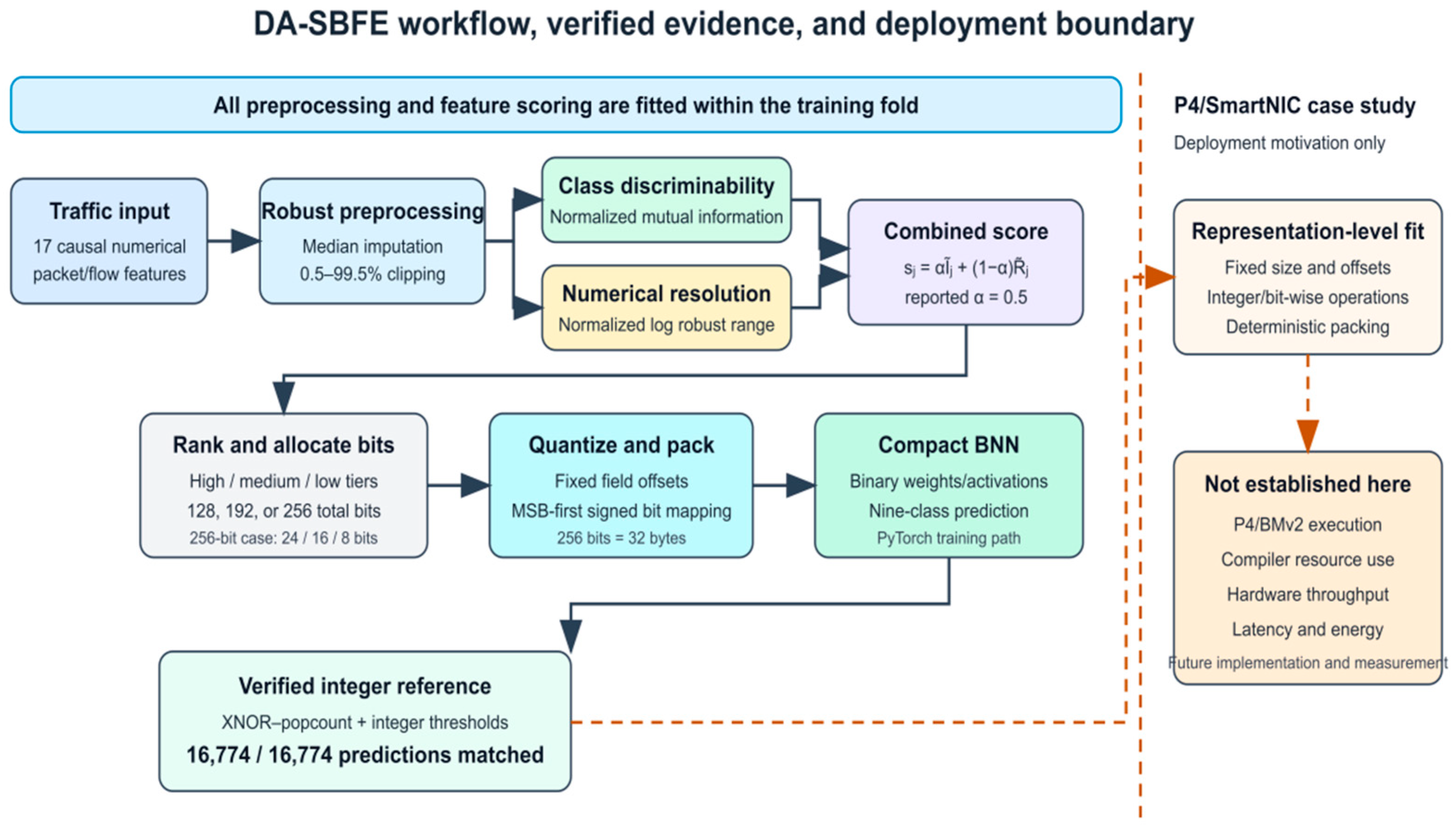
Figure 1 summarizes the leakage-safe fitting path, the compact BNN inference path, the verified deterministic integer check, and the boundary of the P4/SmartNIC case study. Encoder statistics and bit allocation are fitted within each training fold. The 256-bit representation is byte-aligned; the 128- and 192-bit sensitivity settings use proportional widths. The deterministic integer XNOR–popcount path is verified against PyTorch, whereas P4/BMv2 execution and hardware measurements remain future work.

3.2. Fixed-Budget Feature-Encoding Problem

The system uses the UNSW-IoT dataset, which contains real network-traffic captures from genuine IoT devices. Consider a training set ${\mathcal{D}}_{\mathcal{t}\mathcal{r}}={\left(x_i,y_i\right)}_{i=1}^N$, where $x_i\in R^d$ contains $d$ causal numerical traffic features and $y_i\in 1,\dots ,C$ is the device-class label. In the present study, $d=17$ and $C=9$. The purpose of the encoder is to transform each continuous feature vector into a signed binary vector of fixed length B:

$$E_B:R^d\to -1,+1^B.$$

Let $b_j$ denote the number of bits allocated to feature j. The allocation must satisfy ${\sum }_{j=1}^d{b}_j+p=B$, where $p$ is the number of fixed padding bits. For the full 17-feature setting, $p=0$. In the no-port ablation, the 15 retained features occupy 240 bits and the remaining 16 positions are fixed padding bits, preserving the same 256-bit input interface.

A uniform allocation treats all features as equally deserving of precision. A range-based allocation instead favors features with large numerical variation. Neither assumption necessarily agrees with the classification objective: a feature can have a narrow numerical range but still separate the classes effectively, whereas a wide-range feature can contain little class-specific information. DA-SBFE, therefore, treats feature encoding as a constrained allocation problem. It ranks features using both their training-set class discriminability and their robust numerical ranges, assigns one of three precision levels, and then quantizes all features into a single fixed-length bit vector. All parameters of the encoder—including missing-value statistics, clipping bounds, mutual-information scores, feature ranks, and bit widths—are estimated exclusively from the corresponding training fold. They are then held fixed when transforming the validation and test sets.

3.3. Training-Fold Preprocessing and Robust Range Estimation

For each feature j, non-finite training values are replaced by the training-fold median m_j. The same value is retained for later transformation of validation and test data. DA-SBFE then estimates lower and upper bounds from the 0.5th and 99.5th percentiles of the imputed training values: $l_j=Q_{0.005}\left(X_j\right), uj=Q0.995Xj$. An input value is clipped according to $x_{ij}^c=min\left\{max\left(x_{ij},l_j\right),u_j\right\}$.

This percentile operation limits the influence of extreme observations on the quantization interval. It is used as a robustness safeguard; it is not assumed to improve classification accuracy by itself. Because the traffic features are measured on different numerical scales, the raw range is compressed logarithmically: $R_j=log\left[1+max\left(0,u_j-l_j\right)\right]$.

The logarithm prevents features with exceptionally large numerical ranges from dominating the score solely because of their units. Let $\mathcal{N}\left(\cdot \right)$ denote min–max normalization across the retained features:

$$\mathcal{N}\left(a_j\right)=\left\{\begin{array}{cc}{\displaystyle \frac{a_j-\underset{k}{\min }{a}_k}{\underset{k}{\max }{a}_k-\underset{k}{\min }{a}_k}},& \underset{k}{\max }{a}_k>\underset{k}{\min }{a}_k,\\ 0,& \mathrm{otherwise}.\end{array}\right.$$

The normalized range score is consequently ${\tilde{R}}_j=\mathcal{N}\left(R_j\right).$

3.4. Discriminability-Aware Feature Scoring

The numerical range describes the resolution required to represent a feature, but it does not measure how strongly that feature is related to the class label. DA-SBFE incorporates this second consideration through mutual information: $I_j=I\left(X_j^c;Y\right),$ where $X_j^c$ denotes the clipped training-fold values of feature $j$. Mutual information can capture non-linear statistical dependence and does not require a monotonic relationship between a traffic feature and the device class. The resulting values are normalized across the retained features:

$${\tilde{I}}_j=\mathcal{N}\left(I_j\right).$$

DA-SBFE combines the two normalized quantities as

$$s_j\left(\alpha \right)=\alpha {\tilde{I}}_j+\left(1-\alpha \right){\tilde{R}}_j, 0\le \alpha \le 1.$$

The reported DA-SBFE configuration fixes $\alpha =0.5$, giving equal weight to discriminability and robust range. This setting is kept constant throughout the reported main comparisons; it is not adjusted using test-fold performance. The two endpoints provide controlled alternatives: $\alpha =0$ gives Range-SBFE, whereas $\alpha =1$ gives discriminability-only SBFE. Thus, comparisons among these variants modify the ranking criterion, while preserving the downstream quantization and BNN procedures. Features are sorted in descending order of $s_j$. A stable ordering is used when two features receive identical scores, ensuring deterministic allocation.

3.5. Three-Tier Bit Allocation

Let $\pi \left(r\right)$ denote the feature at rank $r$, with $r=1$ corresponding to the highest score. For the 17-feature representation, DA-SBFE divides the ranking into three groups: ranks 1–6 receive high precision, ranks 7–9 receive medium precision, and ranks 10–17 receive low precision. For a total budget $B\in 128,192,256$, define the allocation unit as

$$v_B={\displaystyle \frac{B}{32}}.$$

The bit width assigned to a ranked feature is

$$b_{\pi \left(r\right)}=\left\{\begin{array}{ll}3v_B,& 1\le r\le 6,\\ 2v_B,& 7\le r\le 9,\\ v_B,& 10\le r\le 17.\end{array}\right.$$

The total width is

$$6\left(3v_B\right)+3\left(2v_B\right)+8v_B=32v_B=B.$$

Table 1. The three-tier allocations used for the bit-budget experiments.

Total Budget $\mathit{B}$	Ranks 1–6	Ranks 7–9	Ranks 10–17	Total
128 bits	12 bits/feature	8 bits/feature	4 bits/feature	128 bits
192 bits	18 bits/feature	12 bits/feature	6 bits/feature	192 bits
256 bits	24 bits/feature	16 bits/feature	8 bits/feature	256 bits

summarizes the resulting configurations.

The primary 256-bit configuration is byte-aligned: every feature occupies 8, 16, or 24 bits, and the resulting vector occupies 32 bytes. The 128- and 192-bit configurations are proportional sensitivity settings that preserve the same rank groups; their individual feature widths are not all byte-aligned. This distinction prevents the budget analysis from being interpreted as evidence that every tested representation has the same alignment properties. When source and destination ports are removed, $d=15$. The same six-high-precision, three-medium-precision allocation rule is retained. At $B=256$, the 15 feature fields occupy $6\left(24\right)+3\left(16\right)+6\left(8\right)=240$ bits. Sixteen fixed zero code bits are appended to preserve the 256-bit interface used by the classifier.

3.6. Quantization and Symmetric Bit Mapping

After the bit widths are assigned, each clipped feature value is quantized independently. For a feature receiving $b_j$ bits, its integer code is

$$q_{ij}=\mathrm{r}\mathrm{o}\mathrm{u}\mathrm{n}\mathrm{d}\left[{\displaystyle \frac{x_{ij}^c-l_j}{u_j-l_j}}\left(2^{b_j}-1\right)\right].$$

If $u_j=l_j$, the feature is constant on the training fold and its code is set to zero. Otherwise, $q_{ij}$ lies between $0$ and $2^{b_j}-1$.

The integer is expanded into an MSB-first binary sequence. Its $k$-th bit is

$$c_{ij,k}=⌊{\displaystyle \frac{q_{ij}}{2^{b_j-1-k}}}⌋\hspace{0.25em}\mathrm{m}\mathrm{o}\mathrm{d}\hspace{0.25em}2, k=0,\dots ,b_j-1.$$

Feature fields are concatenated in the original feature order rather than their score order. Ranking controls only the number of bits allocated to each field; it does not alter the semantic layout of the input vector. Consequently, the offset of every feature remains explicit and deterministic.

Finally, the code bits are mapped symmetrically around zero:

$$z_{ij,k}=2c_{ij,k}-1,$$

so that $c_{ij,k}=0$ becomes $-1$ and $c_{ij,k}=1$ becomes $+1$. Concatenating all signed fields produces

$${\mathbf{z}}_i=E_B\left({\mathbf{x}}_i\right)\in \{-1,+1{\}}^B.$$

The term symmetric in DA-SBFE refers specifically to this $0,1\to -1,+1$ mapping. It does not imply that the original continuous feature distribution or its clipping interval is symmetric about zero. In the no-port ablation, the appended zero code bits, therefore, correspond to fixed $-1$ values after the signed mapping.

3.7. Binary Classifier and Integer XNOR–Popcount Form

The encoded vector is processed by a fully connected BNN. The primary BNN–Large architecture has dimensions

$$B\to 128\to 64\to 9.$$

The hidden and output weights are binarized to $-1,+1$ during the forward pass. Batch normalization and signed activations follow the hidden linear layers, while the final layer produces nine class scores. Training uses latent real-valued weights, a straight-through estimator for the sign function, and weight clipping, following established BNN training practice [14,15].

For signed vectors $\mathbf{a},\mathbf{w}\in \{-1,+1{\}}^K$, their dot product can be evaluated without floating-point multiplication:

$${\mathbf{a}}^{\mathsf{T}}\mathbf{w}=2\hspace{0.17em}\mathrm{p}\mathrm{o}\mathrm{p}\mathrm{c}\mathrm{o}\mathrm{u}\mathrm{n}\mathrm{t}\left[\mathrm{X}\mathrm{N}\mathrm{O}\mathrm{R}\left(\stackrel{\mathbf{‾}}{\mathbf{a}},\stackrel{\mathbf{‾}}{\mathbf{w}}\right)\right]-K,$$

where $\stackrel{\mathbf{‾}}{\mathbf{a}}$ and $\stackrel{\mathbf{‾}}{\mathbf{w}}$ are the corresponding $0.1$ representations. Each hidden neuron can, therefore, be expressed as a comparison between an integer popcount and a precomputed threshold. Batch-normalization parameters are folded into these thresholds after training, and the output class is selected by the largest integer dot product.

This conversion establishes a deterministic integer representation of the trained network.

3.8. Leakage-Safe Fitting and Deployment-Oriented Case Study

DA-SBFE is fitted exclusively on each outer training fold using the specified bit budget and the fixed reported value α = 0.5. For every feature, the training data are first used to estimate the median imputation value and the 0.5th and 99.5th percentile clipping bounds. After imputation and clipping, the normalized log-range and mutual-information values are computed and combined using s_j(0.5). The resulting scores determine the feature ranking and the assignment of the three precision tiers. The fitted encoder state, therefore, consists of the imputation values, clipping bounds, feature ranks, allocated widths, and bit offsets.

When the fitted encoder is applied to a validation, test, or subsequently observed sample, all preprocessing uses this stored state. Each feature is imputed and clipped with the training-fold parameters, quantized at its assigned precision, expanded into an MSB-first code, and finally mapped from {0, 1} to {−1, +1}. No distributional statistic, feature score, rank, or allocation is recomputed from validation or test data. This separation is essential because mutual information uses class labels; estimating it outside the training fold would introduce target leakage.

The resulting 256-bit representation also provides a deployment-oriented P4/SmartNIC case study. Its fixed 32-byte size, predetermined field offsets, binary weights, and integer comparison thresholds define a compact interface based on restricted per-packet operations. These properties motivate examining DA-SBFE in a programmable-data-plane context, but they do not constitute deployment evidence. The present study verifies only the software encoder and deterministic integer XNOR–popcount inference. P4 compilation, BMv2 packet execution, hardware resource consumption, throughput, and latency remain subjects for future implementation and measurement.

4. Experimental Setup

4.1. Dataset Provenance and Cohort Reconstruction

The evaluation used traffic records reconstructed from the official UNSW IoT traces released with the corresponding device-classification study [4]. The source data were collected from a testbed containing consumer IoT devices and were distributed as daily packet captures and processed packet metadata. The primary within-day cohort was reconstructed from the trace recorded on 23 September 2016.

To retain continuity with the original 83,868-sample cohort while restoring verifiable provenance, each retained row was matched to an official packet using its device label and five effective fields preserved in the earlier preprocessing output. Repeated packet tuples were resolved using deterministic reservoir sampling with seed 42. The original row and label order were retained. The reconstruction reproduced the five retained fields exactly for every row, while the remaining constant or unauditable columns from the earlier array were excluded.

The resulting cohort contains nine device classes.

Table 2. The device classes in the reconstructed within-day cohort.

Class	Device	Samples
1	Dropcam	10,000
2	Withings Smart Baby Monitor	10,000
3	Amazon Echo	10,000
4	Netatmo Welcome	10,000
5	Smart Things	10,000
6	Samsung SmartCam	10,000
7	Android Phone	10,000
8	Netatmo Weather Station	7019
9	TP-Link Day Night Cloud Camera	6849
	Total	83,868

reports the corrected device identities and sample counts. The first seven classes contain 10,000 packets each; the final two contain 7019 and 6849 packets, respectively. Consequently, the cohort is moderately imbalanced and is not described as fully balanced.

MAC and IP addresses were used to associate packets with device labels and to construct flow state, but they were not included in the classifier input. This exclusion prevents the model from identifying devices through explicit address information. Seventeen causal numerical features were computed from the time-ordered packet trace. The packet-level fields comprise the UDP indicator, packet size, source port, destination port, and outbound-direction indicator. Accumulated flow features comprise flow age, total packet count, total byte count, inbound and outbound packet counts, and inbound and outbound byte counts. The remaining statistics are the mean packet size, standard deviation of packet size, current inter-arrival time, mean inter-arrival time, and jitter. Every flow statistic uses only the current packet and packets observed earlier in the same flow. No future packet information was introduced.

4.2. Within-Day Validation Protocol

The main comparison used stratified five-fold cross-validation. The folds were generated once using shuffled stratification with random state 42 and were then frozen for all encoders, model-capacity settings, and ablations. Each test fold contains approximately 16,774 packets, while the corresponding training partition contains approximately 67,094 packets.

All data-dependent preprocessing is performed independently within each outer training fold. This includes median imputation, percentile-bound estimation, mutual-information estimation, score normalization, feature ranking, bit allocation, and quantization. The fitted encoder is subsequently applied to the outer test fold without recomputing any statistic. Each BNN configuration is trained with three random seeds: 42, 52, and 62. For reporting, the three seed-level results are first averaged within each outer fold. The final mean and standard deviation are then calculated across the five-fold-level averages. This aggregation prevents the repeated initializations of one fold from being treated as independent test partitions.

The reported DA-SBFE models used $\alpha =0.5$ in every outer fold. During the primary experiment, candidate values of 0.25, 0.50, and 0.75 were evaluated through an inner three-fold split of the outer training partition using a fixed logistic linear proxy. The outer test fold was never accessed during this process, and all five outer folds returned $\alpha =0.5$. The revised manuscript, therefore, reports 0.5 as the common DA-SBFE setting. The no-port and cross-day experiments fix it directly to 0.5.

The frozen folds are packet-level splits. A flow–disjoint alternative was examined, but several device classes were dominated by a small number of large flows, causing some candidate test folds to omit multiple classes. Because such folds cannot provide a complete nine-class comparison, they were not used for model ranking. The primary evidence is therefore limited to within-day, packet-level generalization.

4.3. Compared Encoders and Models

The primary 256-bit comparison includes four encoders:

• Equal-256 assigns 15 bits to each of the 17 features and appends one fixed zero code bit.
• Range-SBFE ranks features only by their normalized robust range, corresponding to $\alpha =0$.
• Disc-SBFE ranks features only by normalized mutual information, corresponding to $\alpha =1$.
• DA-SBFE combines the two components using $\alpha =0.5$.

All four encoders use the same training-fold clipping bounds, scalar quantization rule, bit order, and signed mapping. Thus, their comparison isolates the effect of the allocation criterion rather than changes to the downstream classifier. BNN-Large is the primary classifier. Its architecture is $B$-128-64-9, where $B$ is the encoded input budget. At $B=256$, the implementation contains 41,920 trainable and fixed affine parameters counted by the software framework. BNN-Medium, with hidden widths 64 and 32, is included to examine whether the allocation effect persists when model capacity is reduced.

Two conventional classifiers operating directly on the 17 floating-point features provide numerical references: a decision tree, with maximum depth of 9, and a random forest containing 100 trees, with a maximum depth of 12. Both use the Gini criterion and random state 42. These models are host-side references rather than programmable-data-plane implementations. Their purpose is to contextualize classification performance, not to support P4 resource or throughput comparisons.

4.4. BNN Training Configuration

The BNNs were implemented in PyTorch. Binary weights and signed hidden activations follow the established BNN formulation [14,15]. During the forward pass, each weight is mapped to $-1,+1$. The straight-through estimator passes gradients only for latent values within $\left[-1,1\right]$, and the latent weights are clipped to the same interval after every optimizer update.

Training minimizes nine-class cross-entropy using Adam, with a learning rate of 0.003. The batch size is 512, and the maximum training duration is 15 epochs. Within each outer training fold, 10% of the samples are assigned to a stratified validation subset. Early stopping monitors validation macro-F1 with a patience of four epochs, and the checkpoint with the highest validation score is retained.

The hidden layers use center-only batch normalization: the shift parameter is learned, whereas the scale is fixed to one. The final layer does not apply a signed activation because its nine integer dot products serve as the class scores. The predicted class is the index of the largest score.

The verified software environment includes Python 3.12.13, PyTorch 2.11.0 with CUDA 12.8 support, NumPy 2.5.1, SciPy 1.18.0, and scikit-learn 1.9.0. Training time is not used as evidence of packet-processing latency or hardware efficiency.

Generative AI assistance was limited to language editing, structural revision, and consistency checking. It was not used to generate data, run experiments, select reported outcomes, or calculate the numerical results.

4.5. Evaluation Metrics and Statistical Summaries

Macro-F1 is the primary metric because it assigns equal weight to all nine classes despite their different sample counts. For class $c$, precision $P_c$, recall $R_c$, and F1 score $F{1}_c$ are computed conventionally. Macro-F1 is

$$\mathrm{M}\mathrm{a}\mathrm{c}\mathrm{r}\mathrm{o}\text{-}\mathrm{F}1={\displaystyle \frac{1}{C}}{\displaystyle \sum _{c=1}^C}F{1}_c.$$

A class with no predicted samples receives zero precision and zero F1, rather than being omitted from the average. Balanced accuracy, overall accuracy, macro recall, per-class precision, per-class recall, per-class F1, and confusion matrices are reported as secondary measures. In this single-label nine-class setting, balanced accuracy is equivalent to the mean of the class recalls.

Encoder comparisons are paired by outer fold. Let $d_k$ denote the difference between DA-SBFE and a comparison encoder on fold $k$, after averaging the three training seeds. The reported paired gain is

$$\bar{d}={\displaystyle \frac{1}{5}}{\displaystyle \sum _{k=1}^5}{d}_k.$$

Descriptive 95% confidence intervals were calculated from the five paired differences using Student’s t distribution. Exact two-sided Wilcoxon signed-rank tests were also calculated where relevant, but they were interpreted cautiously because five pairs permit only coarse significance levels. The analysis, therefore, emphasizes effect magnitude, confidence intervals, and the consistency of the difference direction across folds.

4.6. No-Port and Cross-Day Protocols

The no-port ablation removes only source and destination ports. It retains the same 83,868 packets, corrected labels, frozen five folds, training seeds, and BNN-Large configuration. The remaining 15 features occupy 240 bits, followed by 16 fixed zero code bits. This preserves the 256-bit model interface while preventing the result from being attributed solely to port values.

The temporal-transfer experiment uses two official daily traces. Training uses 5000 packets from each class on 23 September 2016, producing 45,000 training packets. Testing uses a separate set of 5000 packets per class from 5 October 2016, also totaling 45,000 packets. Median values, clipping bounds, mutual information, feature scores, bit widths, and quantization parameters are fitted on the earlier date and applied unchanged to the later date.

The same physical device instances occur on both dates. This experiment, therefore, measures cross-day temporal transfer, not generalization to unseen devices. Range-SBFE and DA-SBFE are evaluated with the matched seeds 42, 52, and 62. The means and standard deviations are calculated across these three seeds, while confidence intervals over the three paired differences are treated as descriptive because of the small sample size.

5. Experimental Results and Analysis

5.1. Main 256-Bit Comparison

Table 3. The main 256-bit results. The values are the mean ± standard deviation across the five outer folds after averaging the three training seeds within each fold.

Input	Classifier	Macro-F1	Balanced Accuracy	Accuracy
Equal-256	BNN-Large	0.9155 ± 0.0033	0.9150 ± 0.0034	0.9121 ± 0.0033
Range-SBFE	BNN-Large	0.9185 ± 0.0020	0.9182 ± 0.0023	0.9157 ± 0.0023
Disc-SBFE	BNN-Large	0.9306 ± 0.0034	0.9306 ± 0.0034	0.9273 ± 0.0037
DA-SBFE	BNN-Large	0.9330 ± 0.0019	0.9328 ± 0.0020	0.9303 ± 0.0024
Floating-point features	Decision tree	0.8785 ± 0.0026	0.8719 ± 0.0029	0.8705 ± 0.0032
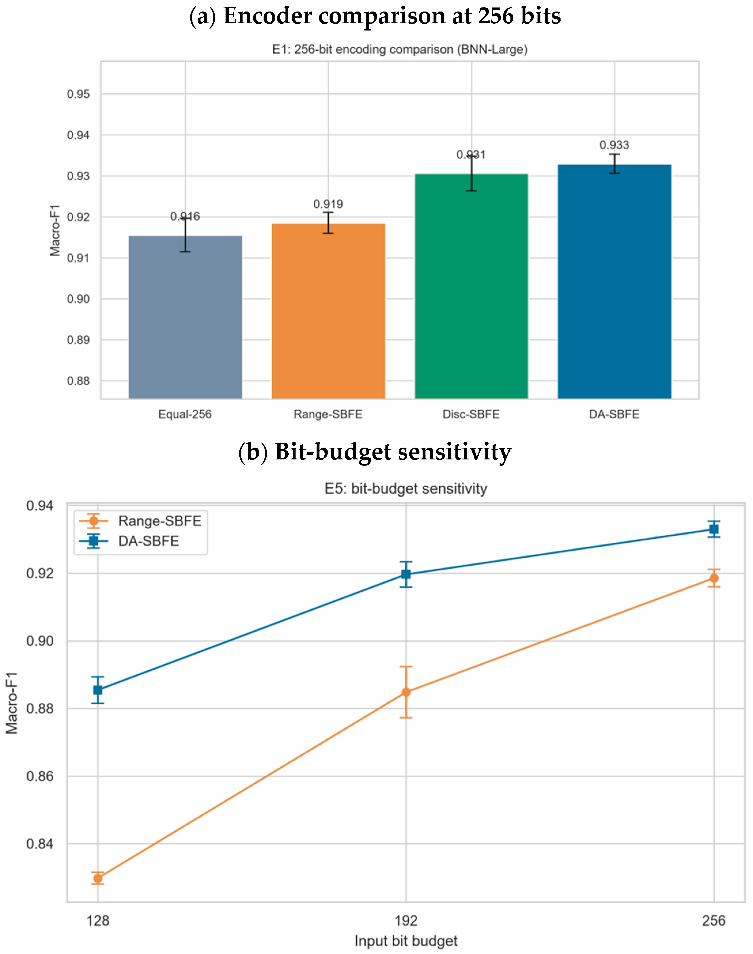
Floating-point features	Random forest	0.9540 ± 0.0020	0.9521 ± 0.0024	0.9498 ± 0.0021

compares the four fixed-bit encoders using the same 256-bit input budget and BNN-Large classifier. DA-SBFE achieved a macro-F1 score of 0.9330 ± 0.0019, compared with 0.9185 ± 0.0020 for Range-SBFE and 0.9155 ± 0.0033 for Equal-256. Its balanced accuracy and overall accuracy followed the same pattern.

Relative to Range-SBFE, DA-SBFE improved macro-F1 by 0.01443. The descriptive 95% confidence interval for the five paired fold differences was [0.01266, 0.01620], and the difference was positive in all five folds. The corresponding balanced-accuracy gain was 0.01460 and was also positive in every fold. These results support the central claim that range alone is an insufficient allocation criterion under the same 256-bit interface.

DA-SBFE also exceeded Equal-256 by 0.01741 macro-F1, with a descriptive 95% confidence interval of [0.01343, 0.02140] and positive differences in all folds. Consequently, the observed gain cannot be explained solely by moving away from a particular range-based ranking; in this experiment, allocating precision according to task-related feature information was preferable to treating the 17 inputs uniformly.

The distinction from discriminability-only allocation was narrower. DA-SBFE exceeded Disc-SBFE by 0.00236 macro-F1 on average, but the paired confidence interval [−0.00104, 0.00576] included zero, and DA-SBFE performed better in four of the five folds. The experiment, therefore, establishes the value of incorporating discriminability relative to range-only allocation, but it does not establish that the additional range term is consistently better than discriminability alone.

The exact two-sided Wilcoxon signed-rank test for the DA-SBFE versus Range-SBFE comparison yielded p = 0.0625. With only five paired folds, this is the smallest attainable two-sided value when every difference has the same direction. We therefore interpret the fold consistency and effect interval descriptively rather than declaring significance from this coarse test.

The floating-point random forest achieves the highest absolute macro-F1, $0.9540\pm 0.0020$. DA-SBFE is not presented as a state-of-the-art host-side classifier. Its contribution is a more effective allocation of a constrained binary input budget for compact integer BNN inference.

5.2. The Effect of the Input Bit Budget

The benefit of discriminability-aware allocation increased as the input budget decreased. As shown in

Table 4. Bit-budget sensitivity of Range-SBFE and DA-SBFE with BNN-Large.

Budget	Encoder	Macro-F1	BNN Parameters	DA Minus Range
128 bits	Range-SBFE	0.8298 ± 0.0014	25,536	—
	DA-SBFE	0.8854 ± 0.0031	25,536	+0.0556
192 bits	Range-SBFE	0.8848 ± 0.0061	33,728	—
	DA-SBFE	0.9196 ± 0.0030	33,728	+0.0348
256 bits	Range-SBFE	0.9185 ± 0.0020	41,920	—
	DA-SBFE	0.9330 ± 0.0019	41,920	+0.0144

, as shown in Table 4, at 128 bits, DA-SBFE improved macro-F1 from 0.8298 to 0.8854, yielding a paired gain of 0.05563. At 192 bits, the gain was 0.03483. It decreased to 0.01443 at 256 bits, where both encoders retained more feature resolution.

The descriptive 95% confidence intervals for the paired gains were [0.05188, 0.05939], [0.02859, 0.04106], and [0.01266, 0.01620] at 128, 192, and 256 bits, respectively. DA-SBFE performed better in all five folds at every budget.

This monotonic reduction in the gain as the budget expands is consistent with the proposed mechanism. Under a tight budget, assigning too many bits to a wide range but weakly discriminative feature directly removes resolution from more useful features. Additional bits reduce that competition. DA-SBFE is, therefore, most beneficial in the resource-constrained regime for which the allocation problem is intended.

Figure 2 jointly summarizes the main 256-bit encoder comparison and the stronger DA-SBFE advantage under tighter input budgets.

5.3. Interaction with BNN Capacity

The same pattern appeared when the classifier was narrowed. As shown in

Table 5. Interaction between feature encoding and BNN capacity at 256 bits.

Classifier	Range-SBFE Macro-F1	DA-SBFE Macro-F1	DA Minus Range
BNN-Medium, 256-64-32-9	0.8755 ± 0.0053	0.9073 ± 0.0033	+0.0318
BNN-Large, 256-128-64-9	0.9185 ± 0.0020	0.9330 ± 0.0019	+0.0144

, with BNN-Medium, Range-SBFE achieved 0.8755 ± 0.0053 macro-F1, whereas DA-SBFE achieved 0.9073 ± 0.0033. The paired gain was 0.03183, with a descriptive 95% confidence interval of [0.02408, 0.03957]. Every fold favored DA-SBFE.

For BNN-Large, the corresponding gain was 0.01443. The advantage, therefore, persists across both tested architectures but is larger for the lower-capacity model.

This result does not imply that encoding can replace model capacity. Both encoders improve when the larger network is used. Instead, it indicates that inefficient bit allocation is more costly when the classifier has less capacity to compensate for information lost at the input interface.

5.4. Score Composition, Alpha Sensitivity, and Clipping

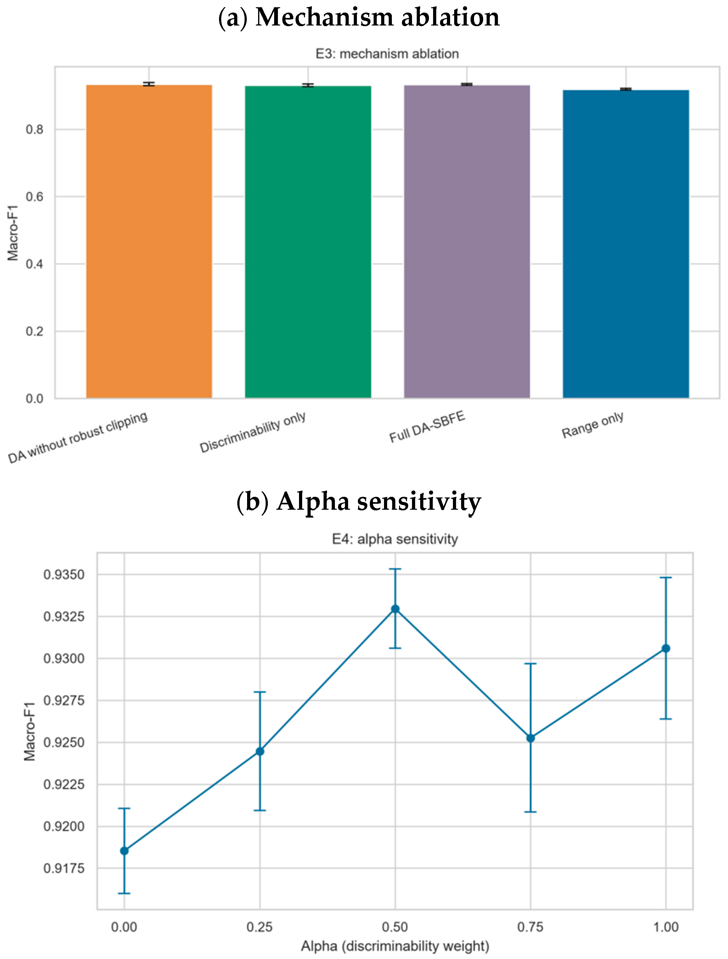
The score ablation separated the contributions of numerical range and class discriminability. Range-only allocation achieved 0.9185 ± 0.0020 macro-F1, whereas discriminability-only allocation achieved 0.9306 ± 0.0034. Their difference shows that the principal improvement over Range-SBFE came from incorporating label-related information into feature ranking.

The response to $\alpha$ is non-monotonic. Macro-F1 values were 0.9185, 0.9245, 0.9330, 0.9253, and 0.9306 for $\alpha =0$, 0.25, 0.50, 0.75, and 1.0, respectively. The equal-weight setting gives the highest mean in this sensitivity analysis, but its paired advantage over $\alpha =1$ remains uncertain because the interval crosses zero. The appropriate conclusion is, therefore, narrower: intermediate weighting is competitive, while discriminability supplies the main improvement over range-only allocation.

As shown in

Table 6. Scoring and clipping ablations at 256 bits.

	Macro-F1	Interpretation
$\mathrm{Range} \mathrm{only}, \alpha =0$	0.9185 ± 0.0020	No label information
$\mathrm{Combined}, \alpha =0.25$	0.9245 ± 0.0028	Range-dominant score
$\mathrm{DA}\text{-}\mathrm{SBFE}, \alpha =0.50$	0.9330 ± 0.0019	Equal-weight setting
$\mathrm{Combined}, \alpha =0.75$	0.9253 ± 0.0036	Discriminability-dominant score
$\mathrm{Discriminability} \mathrm{only}, \alpha =1$	0.9306 ± 0.0034	No range term
DA-SBFE without clipping	0.9339 ± 0.0038	Training-fold extrema

, removing percentile clipping yielded 0.9339 ± 0.0038 macro-F1, compared with 0.9330 ± 0.0019 for the complete DA-SBFE pipeline. Full DA-SBFE minus the no-clipping variant was −0.00097, with a descriptive 95% confidence interval of [−0.00369, 0.00176]. Robust clipping showed no identifiable average accuracy benefit on this trace. It was retained to bound the quantization range in the presence of extreme values, not as an empirically established source of the classification gain. These trends are also illustrated in Figure 3.

5.5. Allocation Stability and Class-Level Effects

The DA-SBFE feature ranking was stable across the five training folds. The outbound byte count, total flow byte count, inbound byte count, source port, destination port, and mean packet size occupied the six 24-bit positions in every fold. Jitter, packet-size standard deviation, and mean inter-arrival time consistently received 16 bits. The remaining eight features received eight bits. This stability indicates that the tier assignments are not being driven by isolated test-fold fluctuations.

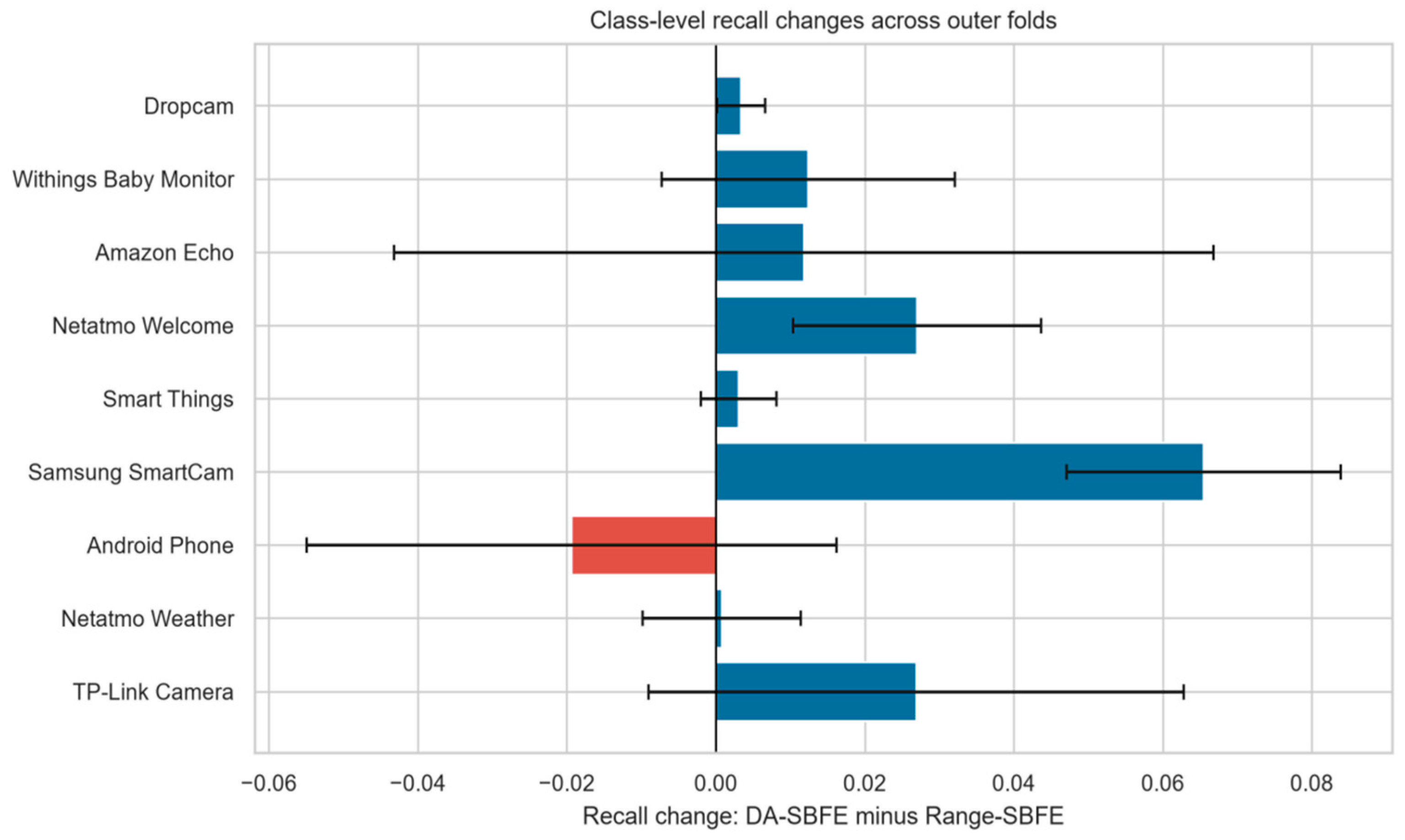
The improvement was not uniform across device classes. Relative to Range-SBFE, DA-SBFE increased Samsung SmartCam recall by 0.0655, with a descriptive 95% confidence interval of [0.0471, 0.0839]. Netatmo Welcome recall increased by 0.0270, with an interval of [0.0103, 0.0437]. Both differences were positive in all five folds. Dropcam showed a smaller increase of 0.0034.

Android Phone recall decreased by 0.0194 on average, although its interval [−0.0549, 0.0162] crossed zero. Other classes showed smaller or less consistent changes. DA-SBFE should, therefore, be interpreted as improving class-balanced aggregate performance, not as guaranteeing higher recall for every device class.

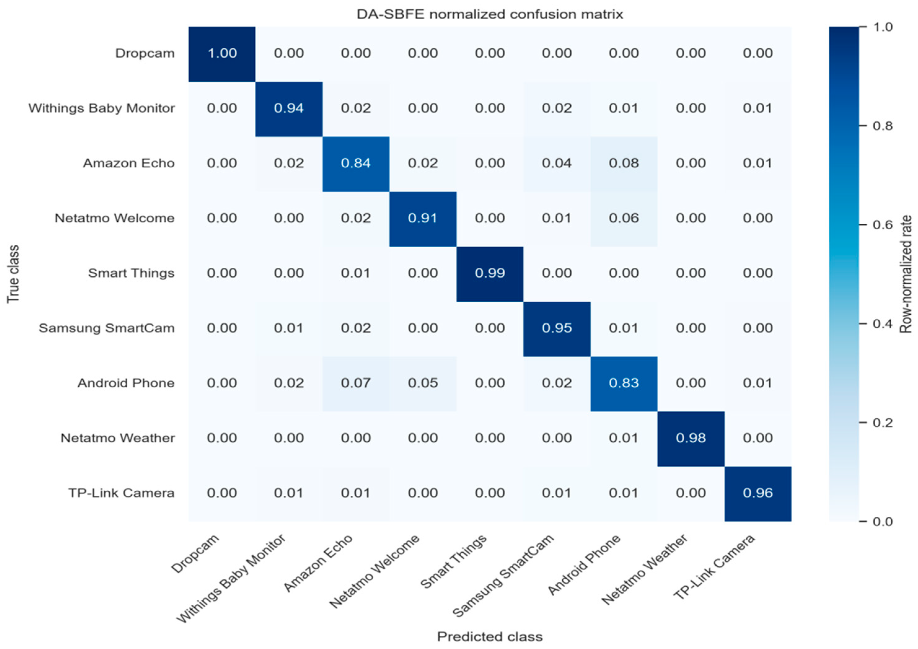
Figure 4 and Figure 5 show the aggregate class structure behind macro-F1. The confusion matrix is averaged after row normalization over all 15 DA-SBFE runs (five folds by three seeds), while the recall-difference panel uses paired outer-fold summaries.

5.6. Ablation Without Port Features

Source and destination ports are highly ranked in the full representation, raising the possibility that the observed advantage is primarily a consequence of those two fields. The no-port experiment tests this explanation directly.

After removing both port features, Range-SBFE achieved 0.8861 ± 0.0076 macro-F1, whereas DA-SBFE achieved 0.9037 ± 0.0022. The paired difference was 0.01760, with a descriptive 95% confidence interval of [0.00885, 0.02634], and DA-SBFE performed better in all five folds.

Removing ports reduces the absolute performance of both encoders, confirming that these fields contain useful class information. However, the DA-SBFE advantage remains after they are removed and is slightly larger in mean magnitude. The benefit of discriminability-aware allocation is therefore not solely driven by source and destination ports.

5.7. Cross-Day Temporal Transfer

As shown in

Table 7. The cross-day transfer from 23 September to 5 October 2016. The values are the mean ± standard deviation across the three matched training seeds.

Encoder	Macro-F1	Balanced Accuracy	Accuracy
Range-SBFE	0.8204 ± 0.0258	0.8200 ± 0.0251	0.8200 ± 0.0251
DA-SBFE	0.8235 ± 0.0194	0.8238 ± 0.0202	0.8238 ± 0.0202

, both encoders showed lower performance when the parameters fitted on 23 September 2016 were transferred unchanged to 5 October 2016. Range-SBFE achieved 0.8204 ± 0.0258 macro-F1, whereas DA-SBFE achieved 0.8235 ± 0.0194. Their balanced accuracies were 0.8200 ± 0.0251 and 0.8238 ± 0.0202, respectively.

The mean paired macro-F1 difference was +0.00317, but the three seed-level differences were +0.04346, −0.00998, and −0.02396. The descriptive 95% confidence interval was [−0.08523, 0.09157]. Two of the three seeds favored Range-SBFE.

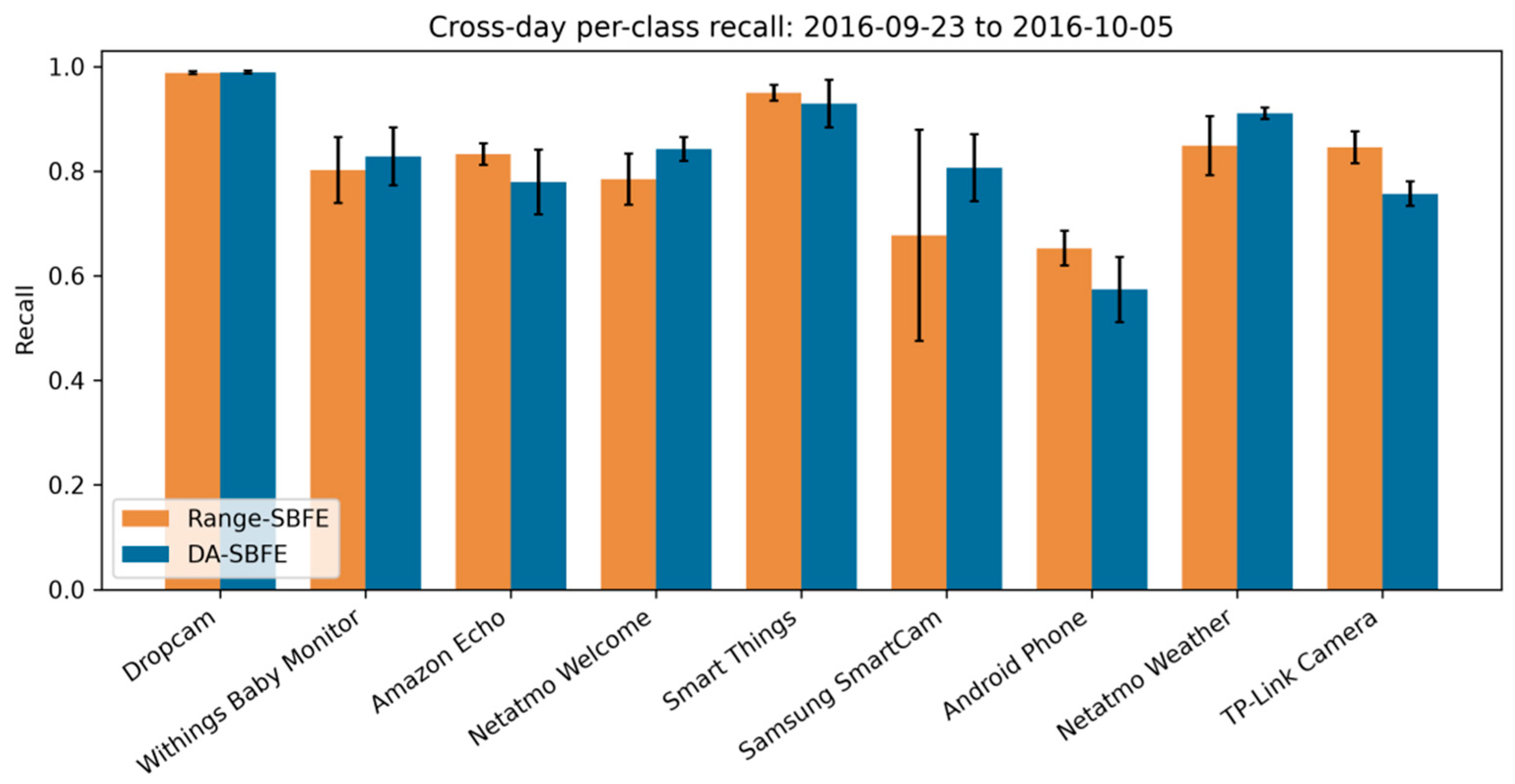
The per-class recall profile is similarly mixed. DA-SBFE improved the mean recall for some devices, including Samsung SmartCam and Netatmo Weather Station, but decreased it for others, including Android Phone and TP-Link Day Night Cloud Camera. This variability is consistent with temporal change affecting device classes differently. The cross-day experiment, therefore, yielded a small positive mean difference but no evidence of a stable DA-SBFE advantage across random initializations. It demonstrates the difficulty of transferring a fixed encoder and classifier across dates. Because the same physical devices appear on both dates, the result must not be interpreted as unseen-device generalization.

Figure 6 confirms that the cross-day class-level effects are mixed rather than uniformly favorable to DA-SBFE. The bars show the mean across the three matched training seeds and the error bars show one standard deviation. The same physical device instances occur on both dates; the comparison is temporal transfer, not unseen-device generalization.

6. Conclusions

This study introduces DA-SBFE, a feature-encoding method that reformulates a fixed-length binary representation as a discriminability-aware bit-allocation problem. By combining training-fold mutual information with a robust numerical range, DA-SBFE assigns byte-aligned precision tiers to heterogeneous traffic features and provides compact BNNs with a more informative binary input under a fixed resource budget. On 83,868 packets from the UNSW IoT traces, DA-SBFE achieved a macro-F1 score of 0.9330 ± 0.0019 at 256 bits, improving on Range-SBFE by 0.0144 across all five folds. The gain increased to 0.0348 at 192 bits and 0.0556 at 128 bits, indicating that discriminability-aware allocation became more valuable as the input budget tightened. The improvement also remained after port features were removed. Moreover, deterministic integer XNOR–popcount inference reproduced all 16,774 PyTorch predictions. These results support DA-SBFE as an effective encoding interface for compact integer classifiers and provide a practical basis for future P4/SmartNIC implementation.