Analytical Kinematic Modelling and Numerical Cross-Verification of a Planar Linkage Mechanism with Linear Actuation

Abstract

Space-constrained articulated mechanisms integrated into mechatronic assemblies require rigorous kinematic characterisation during preliminary design, since spatial limitations and the avoidance of kinematic locking in the transient regime constrain the admissible geometry. An original planar guidance-and-retraction linkage is analysed, composed of three fixed joints, a linear hydraulic actuator, a rigid block of six interconnected elements, and two guiding links that suppress the out-of-plane degrees of freedom; the retractable landing gear of a light training aircraft is adopted as the application case. All mobile joints are expressed in closed form as explicit functions of a single input parameter, the actuator length, without decomposition into Assur groups or iterative compatibility equations. The analytical positions, velocities and accelerations were cross-verified against two independent packages, Linkage v.3.16.14 and GIM v.2025.4; deviations remain below 0.25% of the amplitude of each quantity, with velocity root-mean-square deviations below 0.16 mm/s. The guiding dyad reaches neither dead-centre over the stroke, although its link lengths are treated as preliminary because the 35° minimum transmission-angle margin is not maintained over the first 2.2% of the stroke, for which a corrective dimensioning is provided. The closed-form characterisation provides a basis for subsequent structural, dynamic and experimental analysis.

1. Introduction

The integration of articulated structures into mechatronic systems is constrained by the spatial limitations of the assembly architecture, as in electric-vehicle suspensions [1] and retractable aeronautical landing gears, whose design proceeds from conceptual topology to kinematic identification and numerical analysis [2], correlating link geometry with the dynamic response while avoiding interference with the fixed structure [3,4,5]. In planar-mechanism synthesis, joint number and dimensions are optimised beyond rotational-joint models by integrating prismatic joints through rigid-block discretisation of the synthesis domain [2], with connectivity governed by double-spring models whose stiffness variation fixes the topology and locates geometric singularities of hydraulically actuated retractable gears [2,6,7].

For light training aircraft, landing-gear design requires the dynamic behaviour under impact loads to be established, geometric-parameter optimisation governing reliability and service life under cyclic loading [8,9,10]; topological optimisation reduces design variables through movable morphable elements, whose terminal-point representation yields crossed-bar configurations beyond spring-connected models [9,11,12]. Design-space nonlinearity with global optimisers such as Bayesian algorithms supports trajectory synthesis for four- and six-bar mechanisms, direct analytical modelling eliminating classical decompositions and enabling target XOY trajectories while suppressing transient blockage [12,13,14,15,16].

In the aeronautical field, mass distribution has been correlated with retraction kinematics [17], and ground-contact vibrations attenuated by four-bar mechanisms with helical elements [18,19,20]; related work added momentum-exchange shock absorbers [21], set a minimum transmission angle γ_min = 35° against locking [12], and proposed double-latch anti-drag systems [22]. Unified modelling by plane vector-closure equations replaces Assur decomposition and reproduced a four-bar trajectory with a six-bar Stephenson mechanism [23,24,25,26], analytical and software results agreeing within a few percent [15], while controlled link-length adjustment lowered peak acceleration and inertial loads on bearings and fasteners [24,25,26,27,28].

Pull- and push-type actuation shift the points of maximum velocity with the input angle, relocating stress concentrators [24,29]; the drive configuration alters dynamic stiffness and damping [26], and deformation monitoring enables predictive failure identification transposable to landing gear [29,30]. Correlating closure equations with component stiffness and controlling parasitic OZ deformations suppress locking and limits the inertial loads [29,30,31,32].

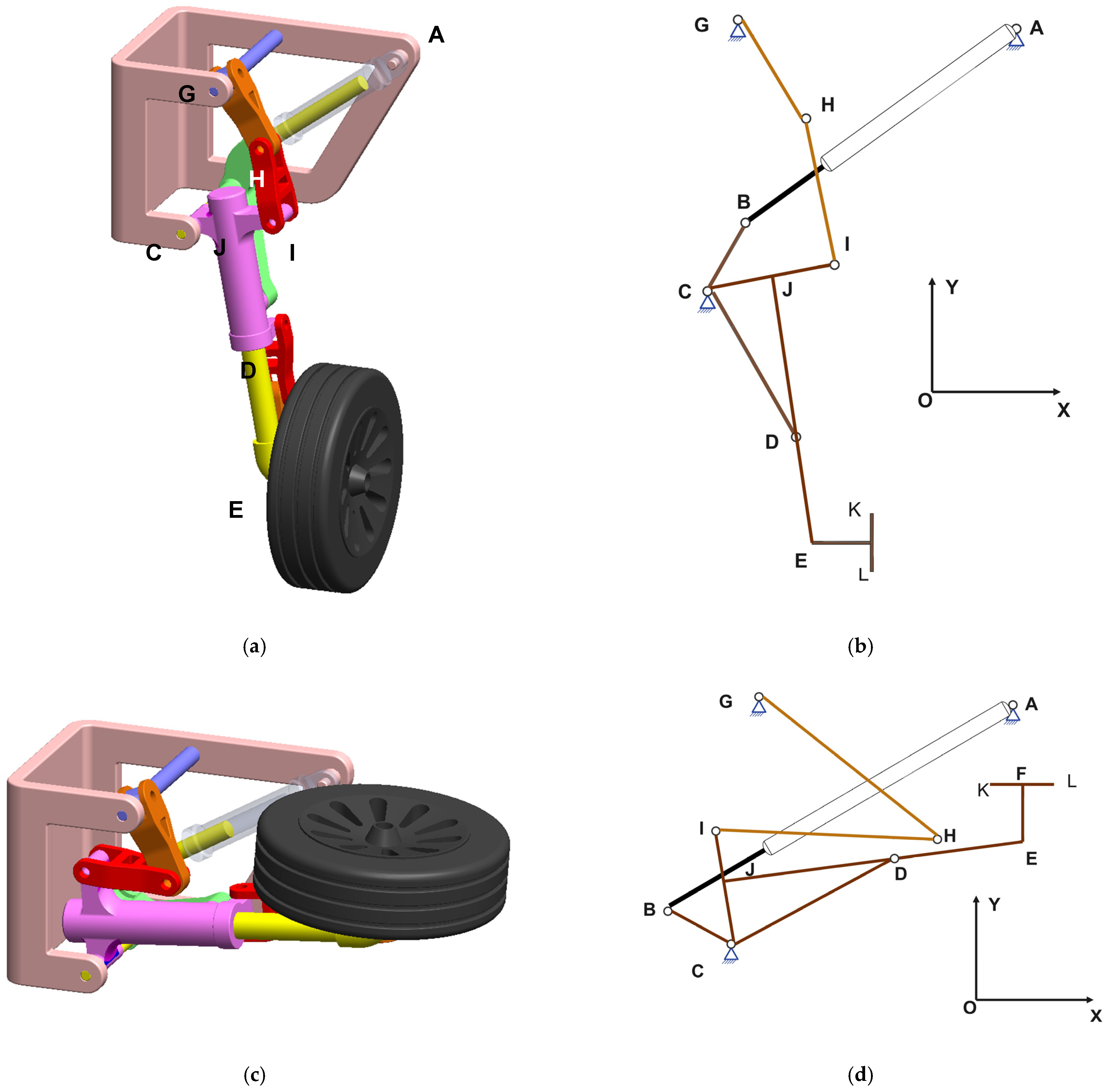
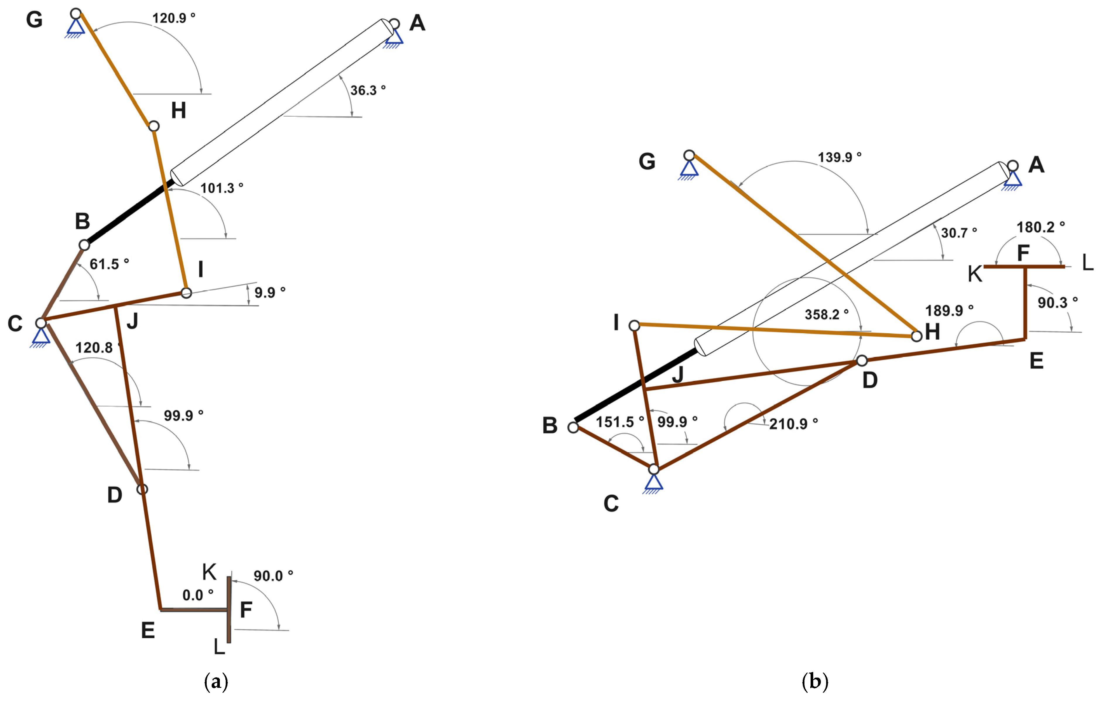
Unlike the two-dimensional planar mechanisms previously analysed by the authors [25,26,27,28] and the landing-gear linkages of [19,20,24], the mechanism proposed here (Figure 1) incorporates two guiding links, GH and HI, restraining the degrees of freedom along the OZ axis.

This out-of-plane restraint legitimises the planar reduction, its counterpart being a passive, unactuated dyad liable to singular configurations in the XOY plane, whose risk is quantified over the whole stroke. The structure omits position-locking devices, its extended and retracted states governed by in-plane positioning.

The topological contribution is therefore condensed into a single formulation: a rigid block of six interconnected members combined with two dedicated guiding links, GH and HI, actuated through a single closed-form input, the actuator length AB, which simultaneously subordinates every mobile trajectory to the single fixed joint C and suppresses the out-of-plane degree of freedom.

As a consequence of the rigid-block topology, six of the nine orientation angles of the model reduce to linear functions of the angles β and δ, and only four require the evaluation of an inverse tangent, which yields a formulation whose computational cost is that of a sequence of explicit evaluations.

A quantitative comparison between the proposed mechanism and a conventional four-bar landing-gear linkage is summarised in

Table 1. Comparison of the proposed retraction mechanism with a conventional four-bar landing-gear linkage and a dual-locking landing-gear linkage.

Criterion	Conventional Planar Four-Bar Linkage	Four-Bar Landing-Gear Linkage (Son et al. [19,20])	Dual-Locking Landing-Gear Linkage (Sung [24])	Proposed Mechanism
Degrees of freedom (M)	1	1	1 +	1 *
Number of mobile links	3	3	+	5 (hydraulic actuator, actuator rod, rigid block, GH, HI)
Number of lower pairs	4 (4R)	4 (4R)	+	7 (6R + 1P)
Actuation mode	rotary/linear input at the crank	static/impact loading; four-bar with helical spring element	pull-type/push-type actuation variants	linear hydraulic actuator (segment AB)
Dedicated in-mechanism OZ restraint	none	none	None	yes, by the guiding links GH and HI
Trajectory subordination to a single fixed joint	none	none	None	yes, rigid block BC–CI–CD–JE–EF–KL
Locking off the working positions	noninherent	none reported	dual locking mechanism	none (governed by in-plane positioning)
Motion plane	XOY	XOY	XOY	XOY, OZ suppressed by GH and HI
Range of motion	crank angular stroke	-	-	actuator extension stroke of 168.6 mm; α from αext = 36.37° (extended, wheel-down) to αret = 30.77° (retracted), minimum 28.9° during the stroke

* For the proposed mechanism, the mobility was evaluated with the rigid block counted as a single body and the hydraulic actuator modelled as a cylinder–rod pair connected by a prismatic joint, which yields M = 1 by the Grübler–Kutzbach criterion; + values reported in [19].

[19,20,24].

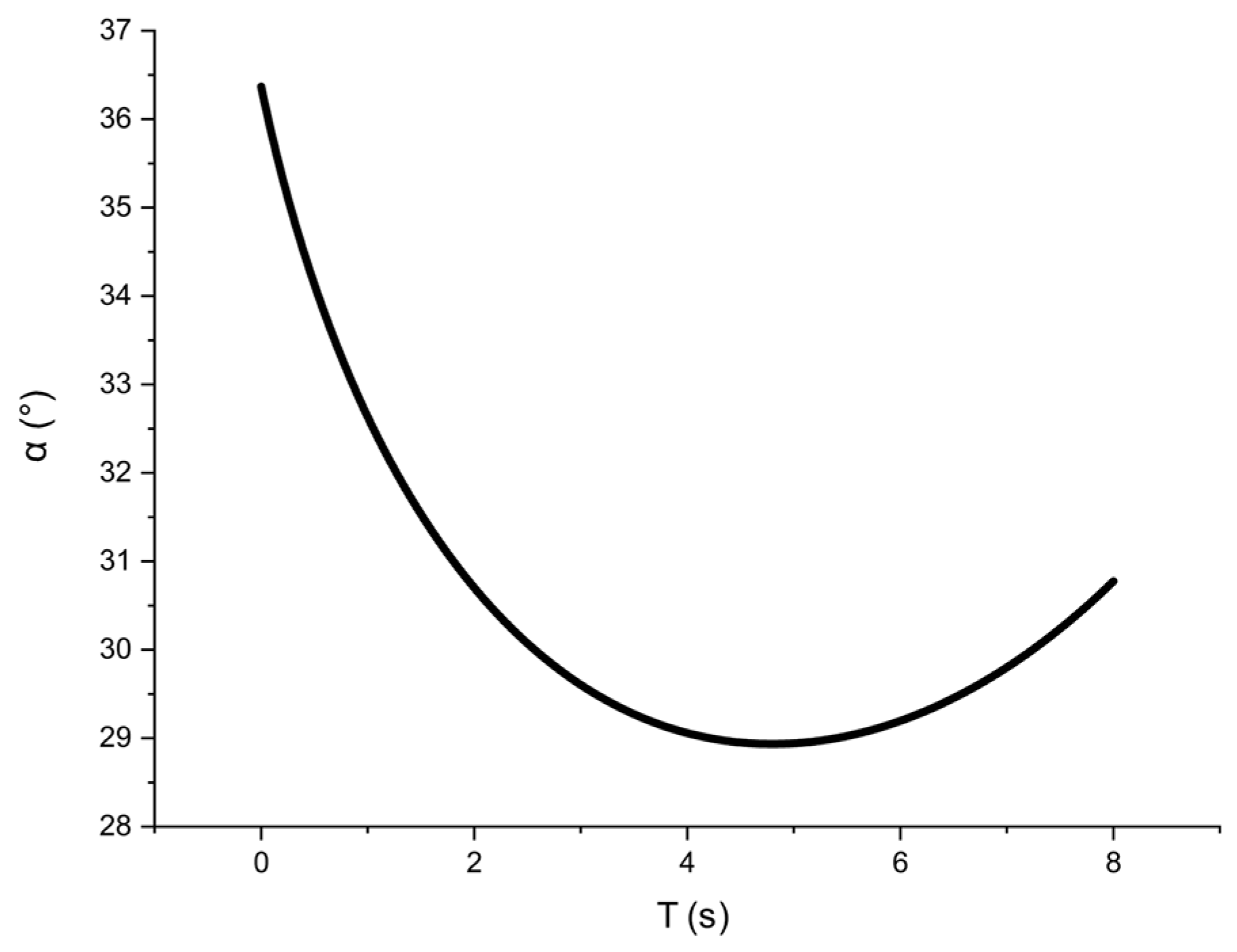
The three features that distinguish the proposed mechanism from the compared landing-gear linkages are quantified as follows. First, both limiting configurations are held by in-plane geometry alone, the actuator covering an extension stroke of 168.60 mm while the input angle α varies from 36.37° in the wheel-down configuration to 30.77° in the wheel-up configuration, with a minimum of 28.9° at mid-stroke; no position-locking device is employed, in contrast with the dual-locking device required by the linkage of Sung [24]. Second, the two dedicated guiding links GH and HI provide a dedicated out-of-plane restraint, the guiding dyad being passive and leaving single-degree-of-freedom mobility unchanged (M = 1 by the Grübler–Kutzbach criterion, for five mobile links and seven lower pairs, six revolute and one prismatic); the four-bar landing-gear linkages of Son et al. [19,20] and the dual-locking linkage of Sung [24] provide no in-mechanism OZ restraint. Third, all mobile trajectories are subordinated to the single fixed joint C through the rigid block BC–CI–CD–JE–EF–KL, rather than being generated through an independent joint; the resulting trajectory of the joint H is non-monotonic, reversing at t = 3.04 s, the distance GI decreasing from 371.30 mm to a minimum of 170.80 mm and the interior angle at H between GH and HI decreasing from 163.9° to 54.2°, a trajectory complexity absent from the compared planar linkages.

2. Materials and Methods

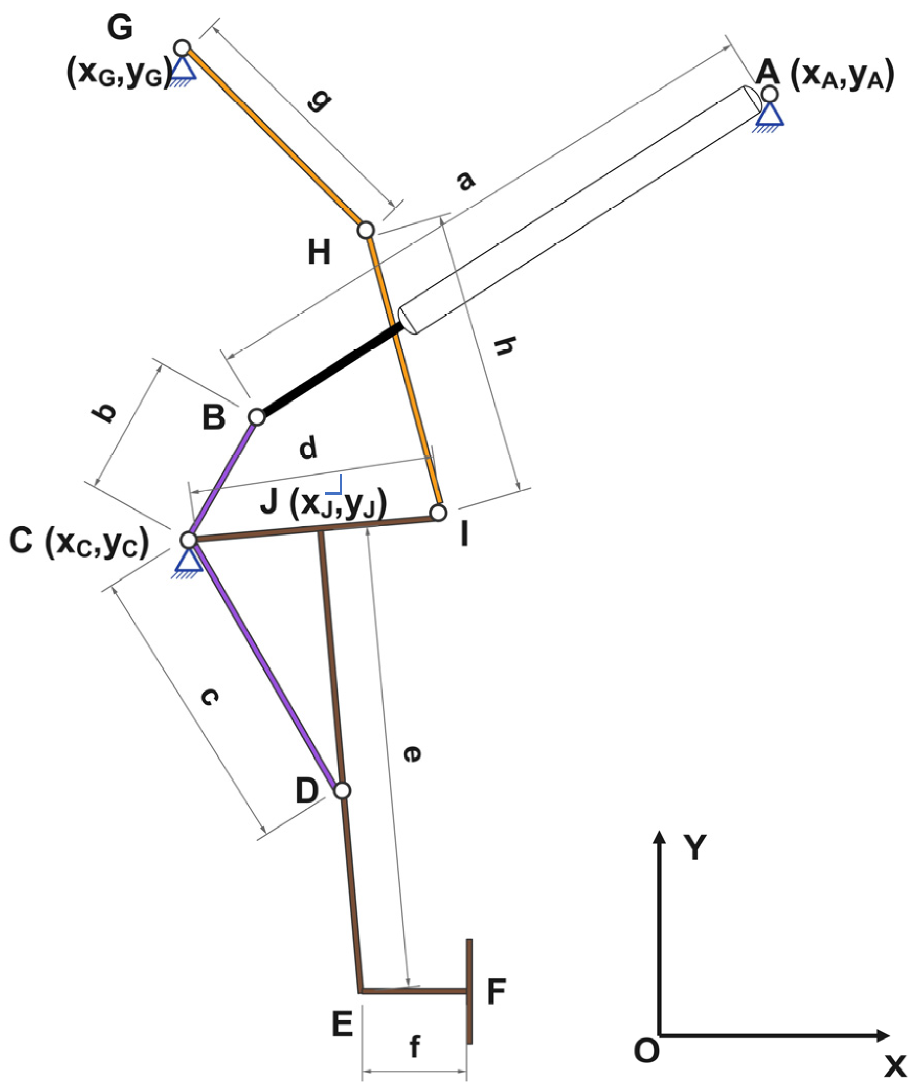
The geometric structure of the analysed mechanism, presented in Figure 2, is defined by means of fixed reference joints, denoted by A, C and G, which ensure the rigid anchoring to the fuselage resistance structure. The motion generating element, responsible for introducing the kinematic flow and the actuating forces into the system, is represented by a hydraulic piston, identified by the articulated segment AB. The movement developed by this linear actuator is transmitted further to a complex kinematic scheme, made up of a rigid assembly formed by the interconnected elements BC, CI, CD, JE, EF and KL [33]. The rigid-body design of this block allows the direct correlation of the trajectories of all the mobile points with the displacement of the piston rod, ensuring an accurate transmission of the loads during the operating phases.

The reduction of the analysis to the XOY plane is admissible because every revolute-joint axis of the assembly is oriented parallel to the OZ axis, so each mobile link is confined to translations and rotations within planes parallel to XOY. Within this planar family of motions, the two guiding links GH and HI form a passive dyad whose addition leaves the single-degree-of-freedom mobility unchanged and which supplies a dedicated out-of-plane restraint: it closes a second support path between the rigid block, at the joint I, and the fixed anchor G, geometrically separated from the block anchorage at the fixed joint C. Any reaction directed along OZ, or any moment about OX or OY applied to the block, is thereby carried through the link HI to the joint H and through the link GH to the fixed anchor G, rather than being reacted at the joint C alone. The quantitative confirmation that the residual out-of-plane displacement under retraction loading remains small relative to the in-plane extension stroke of 168.60 mm requires the deformable-body model and is reserved, together with the fuselage-clearance verification, for the finite-element stage identified in Section 4.

Since the experimental validation on laboratory stands was not carried out at this stage due to logistical unavailability, the numerical verification of the developed mathematical model was carried out by correlating the analytical analysis with computer numerical simulations run in dedicated software packages.

To simulate the movements performed by the drive system of the studied mechanism, the following applications dedicated to the kinematic analysis of mechanisms were used:

-

Linkage v. 3.16.14 is a freeware, developed by a private software writer, intended for the design and simulation of planar mechanisms (2D). It is used for the kinematic analysis of mechanical systems formed by articulated rigid bars [34,35];

-

GIM v. 2025.4 (Graphical Interactive Mechanisms) is an educational software developed by the COMPMECH Research Group (within the University of the Basque Country—UPV/EHU), intended for the analysis and synthesis of planar mechanisms [36,37].

Both packages are planar kinematic tools, which is consistent with the scope of the present study: the mechanism is analysed as a planar, rigid-body system, and the principal result—the admissible design domain of the guiding dyad—is obtained in closed form, the two packages being used solely for the independent cross-verification of the analytical positions, and, in the case of GIM, of the velocities and accelerations. The three-dimensional modelling, dynamic and impact-force capabilities absent from these tools pertain to the deformable-body and load analysis reserved for the finite-element stage identified in Section 4 and are therefore outside the present kinematic scope.

The two packages differ in the kinematic quantities that they return. Linkage computes the successive configurations of the mechanism and exports the coordinates of the joints and is therefore used in the present study for the cross-verification of the trajectories. GIM additionally returns the linear velocities and accelerations of the joints and is consequently the reference used for the cross-verification of the first- and second-time derivatives of the position equations. The comparison of velocities and accelerations reported in Section 3.3 is accordingly restricted to the analytical model and the GIM output; no velocity and acceleration data were derived from the Linkage export, so the compared quantities are in this case produced independently by the two methods.

The three-dimensional assembly of Figure 1 was modelled in SolidWorks 2025 on the basis of the planar sketch of Figure 2, the link lengths, the coordinates of the fixed joints and the fixed angles of the rigid block being those of

Table 2. Complete set of geometric, kinematic and numerical parameters of the analysed mechanism.

Symbol	Parameter	Value at t = 0 (Wheel-Down)	Value at t = 8 s (Retracted)	Unit
Fixed joints
(xA, yA)	Anchor of the hydraulic actuator	(616.500, −54.000)	idem	mm
(xC, yC)	Anchor of the rigid block	(200.000, −426.500)	idem	mm
(xG, yG)	Anchor of the guiding dyad	(286.500, −41.500)	idem	mm
d0	Distance AC, Equation (5)	558.774	idem	mm
Link lengths
a	Actuator AB (variable)	443.593	idem	mm
b	BC	124.496	idem	mm
c	CD	257.003	idem	mm
d	CI	223.801	idem	mm
e	JE	655.423	idem	mm
f	EF	162.990	idem	mm
g	GH	190.000	idem	mm
h	HI	184.996	idem	mm
k	KL (F at mid-span, KF = 100.000)	200.000	idem	mm
-	CJ (dependent)	91.542	idem	mm
-	IJ (dependent)	132.259	idem	mm
Fixed angles of the rigid block
θ	Between CI and CD	69.133	idem	°
φ	Between CB and CD	120.725	idem	°
ψ	Between JE and EF	99.949	idem	°
Actuator law of motion
s(t)	443.593 + 21.075t	443.593	612.193	mm
Δs	Extension stroke	168.600	-	mm
$\dot{s}$	Elongation rate (constant)	21.075	idem	mm/s
$\ddot{s}$	Elongation acceleration	0	idem	mm/s2
T	Stroke time	8.000	-	s
Mobile joints
(xB, yB)	Actuator rod end	(259.31, −317.04)	(90.51, −367.24)	mm
(xH, yH)	Guiding dyad joint	(378.88, −207.53)	(345.50, −222.11)	mm
(xI, yI)	Dyad–block joint	(420.43, −387.80)	(161.20, −206.09)	mm
(xJ, yJ)	Projection of D on CI	(290.16, −410.67)	(184.13, −336.34)	mm
(xD, yD)	End of CD	(331.69, −647.20)	(420.64, −294.71)	mm
(xE, yE)	End of JE	(403.50, −1056.22)	(829.63, −222.72)	mm
(xF, yF)	End of EF (axle)	(566.49, −1056.20)	(829.53, −59.73)	mm
(xK, yK)	End of KL	(566.48, −956.20)	(729.53, −59.79)	mm
(xL, yL)	End of KL (dependent)	(566.50, −1156.20)	(929.53, −59.67)	mm
Angular parameters
α	Direction of $\overrightarrow{BA}$ (input angle)	36.37	30.77
β	Direction of $\overrightarrow{CB}$	61.55	151.58
δ	Direction of $\overrightarrow{CI}$	9.96	99.98
ε	Direction of $\overrightarrow{DC}$	120.82	210.85
υ	Direction of $\overrightarrow{HG}$	119.09	108.09
λ	Direction of $\overrightarrow{IH}$	102.98	355.03
γ	Direction of $\overrightarrow{EJ}$	99.96	189.98
τ	Direction of $\overrightarrow{EF}$	0.01	90.03
σ	Direction of $\overrightarrow{FK}$	90.01	180.03
d2	Distance GI, Equation (22)	371.30	206.85 (min. 170.80 at t = 5.82 s)	mm
Numerical parameters of each method
N	Analytical model (Mathcad 15)	500 points; Δt = 16.03 ms; Δs = 0.3379 mm	-	-
N	Linkage v.3.16.14	241 points; Δt = 33.33 ms; Δs = 0.7025 mm	-	-
N	GIM v.2025.4	121 points; Δt = 66.67 ms; Δs = 1.4050 mm	-	-

, at a scale of 1:1 with respect to the dimensional values employed in the analytical model. The two configurations shown correspond to the extended (wheel-down) and the fully retracted (wheel-up) limits of the actuator stroke, each presented as the three-dimensional assembly and its planar kinematic skeleton, so the physical links and their idealised segments are placed in direct correspondence. The analytical model was implemented in Mathcad 15 over 500 stations of the stroke, and the outputs of GIM v.2025.4 and of Linkage v.3.16.14 were exported in tabular form. The exported tables were collated in Microsoft Excel and the graphical representations of a number of figures were generated in OriginPro 10.1 exclusively from these tables, no plotted value being read from the graphical interface of a simulation package.

2.1. Theoretical Considerations

The kinematic analysis of the mechanism involves, first, defining the initial positions of the component elements. To facilitate this analysis, the mechanism is divided into structural groups, each having a specific role in determining the kinematic parameters.

It is emphasised that the term structural group is employed here in an expository sense, to designate the successive stages of the closed-form forward evaluation, and not in the sense of the classical Assur decomposition. No group is solved through its own loop-closure or compatibility equations; each mobile joint is obtained by direct substitution, as an explicit function of the single input parameter and of the constant geometry of the rigid block.

All the trigonometric functions of Equations (1)–(29) take arguments in radians; the angular values are converted to degrees only when reported in the text, in the tables and in the figures.

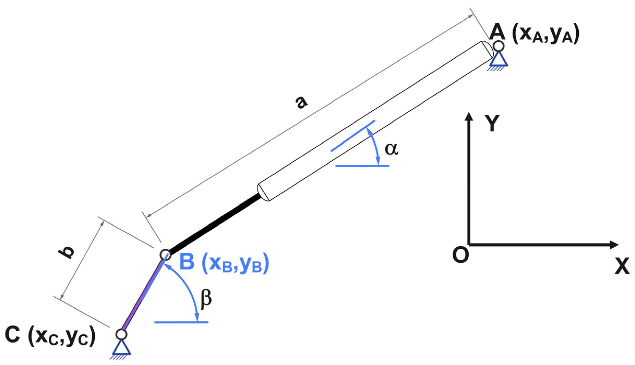
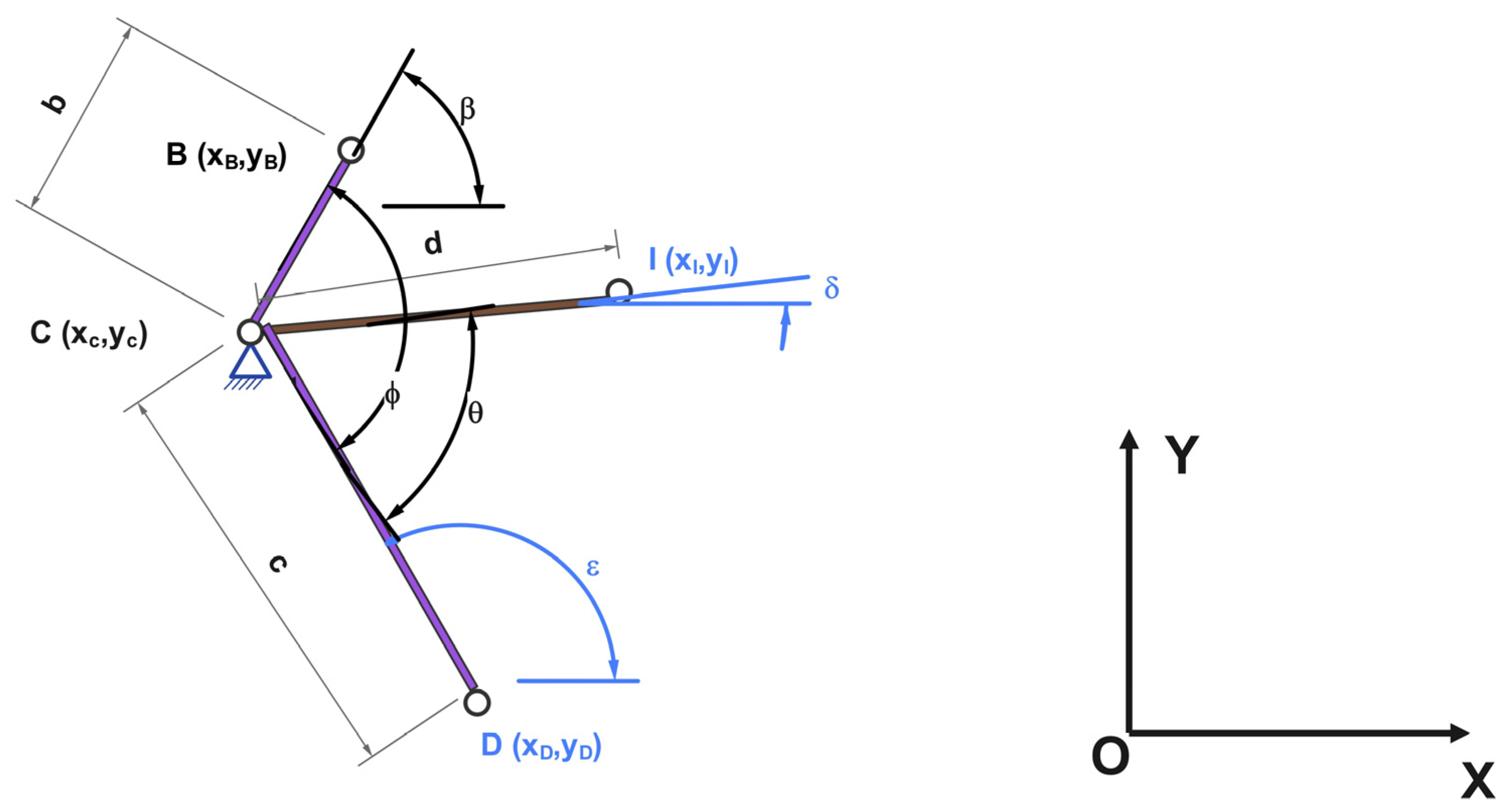
Structural group no. 1—this group (Figure 3) determines the position of the joint B and the orientation angles α and β. Joints A and C are fixed, and B is the movable end of the piston; the coordinates of B follow from the triangle ABC in Equations (1) and (2), the angles α and β from the four-quadrant inverse tangent in Equations (3) and (4), and the auxiliary distances d₀ and d₁ from Equations (5) and (6).

$$x_B={\mathrm{x}}_A+{\displaystyle \frac{(-{\mathrm{x}}_A+{\mathrm{x}}_C)(a^2-b^2+d_0^2)}{2·d_0^2}}-{\displaystyle \frac{d_1·(y_A-y_C)}{2·d_0^2}}$$

(1)

$$y_B={\mathrm{y}}_A-{\displaystyle \frac{(-{\mathrm{x}}_A+{\mathrm{x}}_C)·d_1}{2·d_0^2}}+{\displaystyle \frac{(a^2-b^2+d_0^2)(-y_A+y_C)}{2d_0^2}}$$

(2)

The orientation angles of the actuator and of the binary element CB are obtained with the four-quadrant inverse tangent, from the coordinates of the joints involved:

$$\mathsf{\alpha }=\mathrm{a}\mathrm{t}\mathrm{a}\mathrm{n}2\left(y_A-y_B,x_A-x_B\right)$$

(3)

$$\mathsf{\beta }=\mathrm{a}\mathrm{t}\mathrm{a}\mathrm{n}2\left(y_B-y_C,x_B-x_C\right)$$

(4)

Within these equations, a series of notations were made to reduce their dimensionality. So, d₀ represents nothing more than the distance between points A and C and d₁ is a compound expression that is used to simplify the formulas above.

$$d_0=\sqrt{{({\mathrm{x}}_A-{\mathrm{x}}_C)}^2+{(y_A-{\mathrm{y}}_C)}^2}$$

(5)

$$d_1=\sqrt{a+b-d_0} ·\sqrt{a-b+d_0} ·\sqrt{-a+b+d_0} ·\sqrt{a+b+d_0}$$

(6)

Structural group no. 2—this group (Figure 4) determines the positions of the joints D and I and the orientation angles δ and ε. Elements BC, IC and DC are rigidly connected at the fixed joint C, so the angles ϕ and θ between them are constant; the coordinates of D and I follow from Equations (7)–(10), and the angles δ and ε from Equations (11) and (12).

The horizontal and vertical position of point D, located at the end of element CD, depending on the angle between BC and CD, is determined using the following equations:

$$x_D=x_C+c·\mathrm{c}\mathrm{o}\mathrm{s}(\beta -\varphi )$$

(7)

$$y_D=y_C+c·\mathrm{s}\mathrm{i}\mathrm{n}(\beta -\varphi )$$

(8)

Correspondingly, regarding point I, which is the end of element CI, its position (regardless of the axis to which we refer) depends on the coordinates of the fixed joint C and the values of the imposed angles, respectively:

$${x_I=x}_C+d·\mathrm{c}\mathrm{o}\mathrm{s}\left(\beta +\theta -\varphi \right)$$

(9)

$$y_I=y_C+d·\mathrm{s}\mathrm{i}\mathrm{n}(\beta +\theta -\varphi )$$

(10)

The angle δ represents the angle describing the orientation of the CI element with respect to the OX axis and is determined using Equation (11).

Since the elements BC, CI and CD form a rigid body, the angles θ and ϕ are constant, so the directions of CI and CD follow directly from β:

$$\mathsf{\delta }=\beta +\theta -\varphi$$

(11)

The angle ε represents the orientation of the CD element relative to the OX axis and is calculated with Equation (12), and is a function of the angles generated by the element between BC and the horizontal and the angle between the elements BC and CD.

$$\epsilon =\beta -\varphi +180°$$

(12)

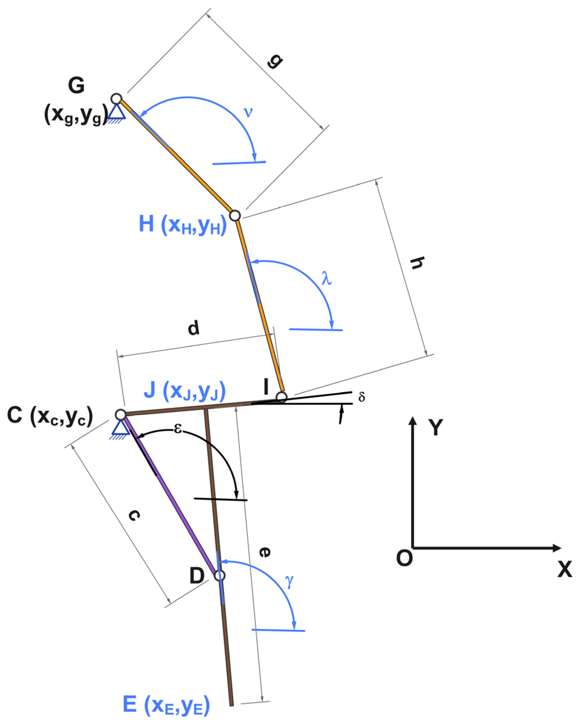
Structural group no. 3—this group (Figure 5) determines the positions of the joints H, J and E and the orientation angles ν, λ and γ. The element EJ is perpendicular to CI, a constraint characterised by the known angle δ; the coordinates of H follow from Equations (13) and (14), those of J and E from Equations (15)–(18), and the angles ν, λ and γ from Equations (19)–(21).

The equations for determining the position on the OX axis and the OY axis of point H are:

$${\mathrm{x}}_H={\displaystyle \frac{(g^2-h^2+d_2^2)·(d·\mathrm{c}\mathrm{o}\mathrm{s}\delta +x_C-x_G)}{2·d_2^2}}+x_G+{\displaystyle \frac{d_3·(-d·\mathrm{s}\mathrm{i}\mathrm{n}\delta -y_C+y_G)}{2·d_2^2}}$$

(13)

$${\mathrm{y}}_H={\displaystyle \frac{d_3·(d·\mathrm{c}\mathrm{o}\mathrm{s}\delta +x_C-x_G)}{2{·d}_2^2}}+{\displaystyle \frac{(g^2-h^2+d_2^2)·(d·\mathrm{s}\mathrm{i}\mathrm{n}\delta +y_C-y_G)}{2·d_2^2}}+y_G$$

(14)

Since the point J belongs to the rigid block and lies, by the orthogonality constraint of the third structural group, on the line CI, its distance from the fixed joint C is invariant along the stroke. Denoting by θ the fixed angle between the elements CD and CI, this distance is the orthogonal projection of CD onto CI, namely $\overline{CJ}=c \cos \theta =91.542 \mathrm{m}\mathrm{m}$, a value which is also recovered from the block geometry as $\overline{CJ}=d-\overline{IJ}$. The coordinates of the joint J are consequently obtained from the direction δ of the element CI, in the same form as those of the joint I:

$$x_J=x_C+c\cos \theta \cos \delta$$

(15)

$$y_J=y_C+c\cos \theta \sin \delta$$

(16)

The equations for the mobile joint E (at the end of the element JE) are obtained using Equations (17) and (18). It is observed that the positioning of this joint is closely related to the coordinates of the joint J but also to the value of the angle δ.

$$x_E=x_J+e\sin \delta$$

(17)

$$y_E=y_J-e\cos \delta$$

(18)

The direction of the guiding links GH and HI results from the coordinates of the joint H, obtained from Equations (13) and (14):

$$\nu =atan2\left(y_G-y_H,x_G-x_H\right)$$

(19)

$$\lambda =atan2\left(y_H-y_I,x_H-x_I\right)$$

(20)

The orthogonality of the element JE to the element CI imposes the direction of JE, so

$$\gamma =\delta +90°$$

(21)

For the dimensional reduction of the equations, a series of notations (Equations (22) and (23)) were made. Therefore, they are presented below:

-

d₂ denoted the distance between the fixed joint G and the mobile joint I, calculated based on the position and angle δ;

-

The equation corresponding to d₃ is an auxiliary expression used to simplify the calculus.

$$d_2=\sqrt{{(-d·\mathrm{c}\mathrm{o}\mathrm{s} \delta -x_C+x_G)}^2+{(-d·\sin \delta -y_C+y_G)}^2}$$

(22)

$$d_3=\sqrt{g+h-d_2}·\sqrt{g-h+d_2}·\sqrt{-g+h+d_2}·\sqrt{g+h+d_2}$$

(23)

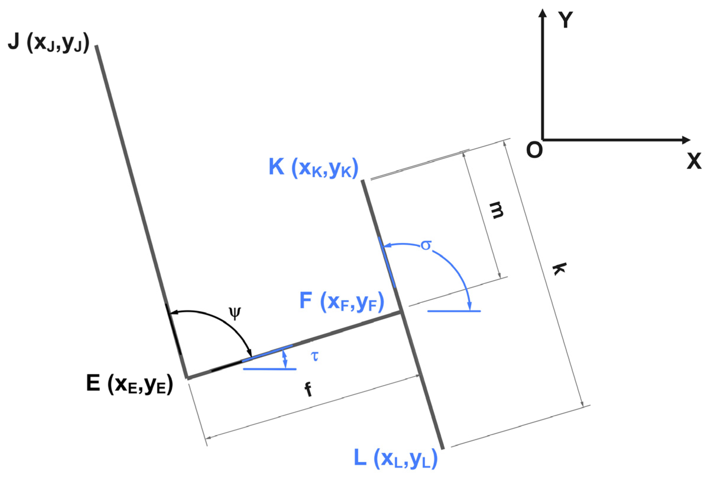
Structural group no. 4—this group (Figure 6) completes the analysis by determining the positions of the movable joints F and K and the orientation angles τ and σ. The element EF forms the fixed angle ψ with JE; the coordinates of F and K follow from Equations (24)–(27), and the angles τ and σ from Equations (28) and (29).

$${x_F=x}_E-{\displaystyle \frac{f·\left(\cos \psi \right(x_E-x_J)-\sin \psi (-y_E+y_J\left)\right)}{\sqrt{x_E^2-2x_E{x}_J+x_J^2+y_E^2-2y_E{y}_J+y_J^2}}}$$

(24)

$${y_F=y}_E-{\displaystyle \frac{f·(-\sin \psi (x_E-x_J)-\cos \psi (-y_E+y_J\left)\right)}{\sqrt{x_E^2-2x_E{x}_J+x_J^2+y_E^2-2y_E{y}_J+y_J^2}}}$$

(25)

$${x_K=x}_F+{\displaystyle \frac{k·(-\sin \psi (x_E-x_J)-\cos \psi (-y_E+y_J\left)\right)}{2·\sqrt{x_E^2-2x_E{x}_J+x_J^2+y_E^2-2y_E{y}_J+y_J^2}}}$$

(26)

$${y_K=y}_F+{\displaystyle \frac{k·\left(\cos \psi \right(-x_E+x_J)+\sin \psi (-y_E+y_J\left)\right)}{2·\sqrt{x_E^2-2x_E{x}_J+x_J^2+y_E^2-2y_E{y}_J+y_J^2}}}$$

(27)

The angles τ and σ follow from:

$$\mathsf{\tau }=\mathsf{\delta }+90°-\mathsf{\psi }$$

(28)

$$\sigma =\tau +90°$$

(29)

2.2. Numerical Parameters of the Model and Simulation Set-Up

The analytical formulation of Section 2.1 expresses every mobile joint as an explicit function of the single input parameter, the actuator length AB, and the constant geometry: the three fixed joints, the link lengths, and the fixed angles of the rigid block. The complete parameter set, which is the sole numerical input of the study and was introduced without modification in Linkage and in GIM, is collected in Table 2; no dimensional or angular value used below is defined outside it. The reference frame is the global XOY plane, with OX directed to the right and OY upwards, all angles measured counterclockwise from the positive OX semi-axis as the direction of the vector named in Table 2. All trigonometric functions in Equations (1)–(29) take arguments in radians, angular values being converted to degrees only for reporting. The actuator motion is prescribed as s(t) = 443.593 + 21.075t mm, an extension stroke of 168.600 mm covered in 8 s at the constant rate $\dot{s}$ = 21.075 mm/s with $\ddot{s}$ = 0; the same law was imposed in Linkage and in GIM, so the three data sets differ only through the number of computed positions and the resulting time step, as listed in the last rows of the table.

Since the positions returned by the analytical model do not depend on the stroke time, the velocities scaling as 1/T and the accelerations as 1/T², the value T = 8 s adopted in Table 2 serves exclusively as a common reference for the three methods compared, whereas the differences between the corresponding time steps, listed in the same table, account for the deviations quantified in Section 3.3.

2.3. Error Metrics and Alignment of the Compared Data Sets

The agreement between the analytical model and the numerical simulations is quantified, for each selected joint and for each kinematic quantity, by four metrics. Denoting by $q_i^{an}$ the value returned by the analytical formulation at the i-th compared sample, by $q_i^{num}$ the corresponding value exported by the simulation software, and by N the number of compared samples, the root-mean-square error (RMSE) and the maximum absolute error (e_max)are defined as:

$$RMSE=\sqrt{{\displaystyle \frac{1}{N}}{\displaystyle {\sum }_{i=1}^N}{\left(q_i^{an}-q_i^{num}\right)}^2}$$

(30)

$$e_{max}=\underset{1\le i\le N}{\max }\left|q_i^{an}-q_i^{num}\right|$$

(31)

and the local percentage error (ε_i), normalised by the analytical value at the same sample, is defined as:

$${\epsilon }_i=100{\displaystyle \frac{\left|q_i^{an}-q_i^{num}\right|}{\left|q_i^{an}\right|}}$$

(32)

The metric of Equation (32) is ill-conditioned wherever the reference value approaches zero, which occurs at the reversal of the trajectory of the joint H, where the velocity vanishes. A percentage error (${\epsilon }_i^{\ast }$) normalised by the amplitude of the quantity over the stroke is therefore introduced as well:

$${\epsilon }_i^{\ast }=100{\displaystyle \frac{\left|q_i^{an}-q_i^{num}\right|}{\underset{1\le i\le N}{\max }\left|q_j^{an}\right|}}$$

(33)

which remains bounded over the whole stroke and is reported together with the maximum and the mean values of ε_i.

Since the three methods discretise the stroke with different steps (Table 2), the analytical quantities, computed at 500 positions, are evaluated at the simulation instants, the comparison being restricted to the common samples, so N = 120 for GIM. Two GIM export conventions are accounted for: the velocity is exported as a signed scalar along the path tangent, changing sign at the reversal of the joint H, so its absolute value is used; and the velocity column is offset by one sample relative to the position and acceleration columns, the initial null being an initialisation marker, so the offset is removed. The alignment was verified on the joint B, whose velocity varies monotonically: its root-mean-square deviation falls from 0.550 mm/s to 0.029 mm/s once the offset is removed, a factor of 19, which identifies the alignment unambiguously. The analytical velocities and accelerations are the closed-form first and second derivatives of the position equations with respect to the actuator length, so no numerical differentiation is involved and no sample is excluded.

3. Results

3.1. Results Obtained Through Mathematical Equations

All the angles of Equations (3), (4), (19) and (20) are returned in the interval (−180°,180°) by the four-quadrant inverse tangent and are subsequently unwrapped, by the addition of integer multiples of 360°, so that they vary continuously along the stroke.

The trajectories of the mobile joints and the associated angular variations were computed in Mathcad 15 over the 500 stroke stations defined in Table 2, under the actuator law of motion prescribed in Section 2.2.

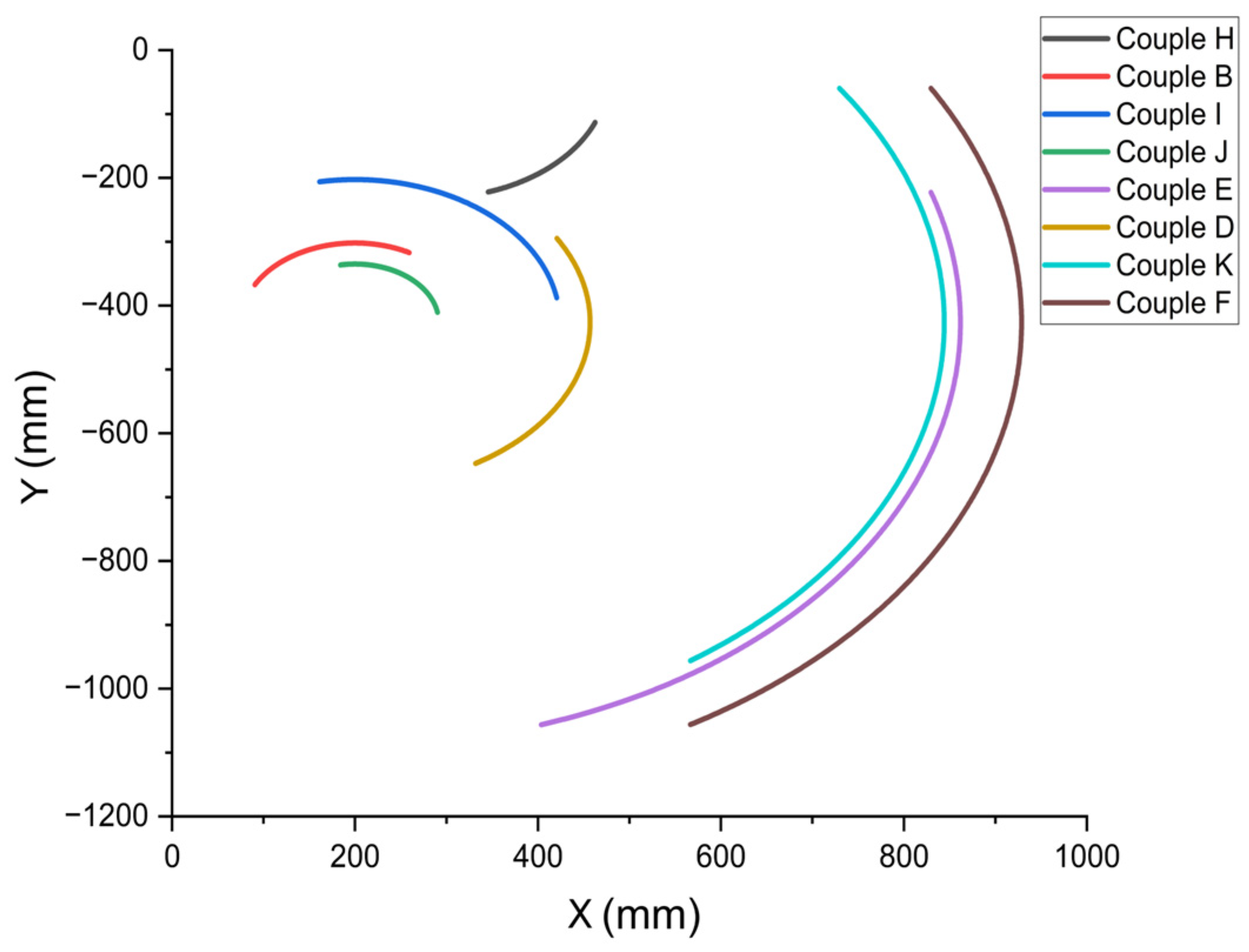
Figure 7 shows that all mobile joints follow arcuate trajectories: the joints B, I, J, E, D, K and L are governed by the fixed joint C, and the joint H by the fixed joint G (Figure 2).

The limiting configurations of the mechanism correspond to both ends of the actuator stroke: in the extended (wheel-down) position, AB = 443.59 mm and α_ext = 36.37°, whereas in the fully retracted position, AB = 612.19 mm and α_ret = 30.77° as presented in Figure 8. The variation in α between these limits is non-monotonic, reaching a minimum of 28.9° at t = 4.79 s. The transmission angle between the actuator axis and the CB crank, evaluated at the joint B, equals 154.8° in the extended configuration and 59.2° in the retracted one, passing through 90° at t = 4.79 s, simultaneously with the minimum of α.

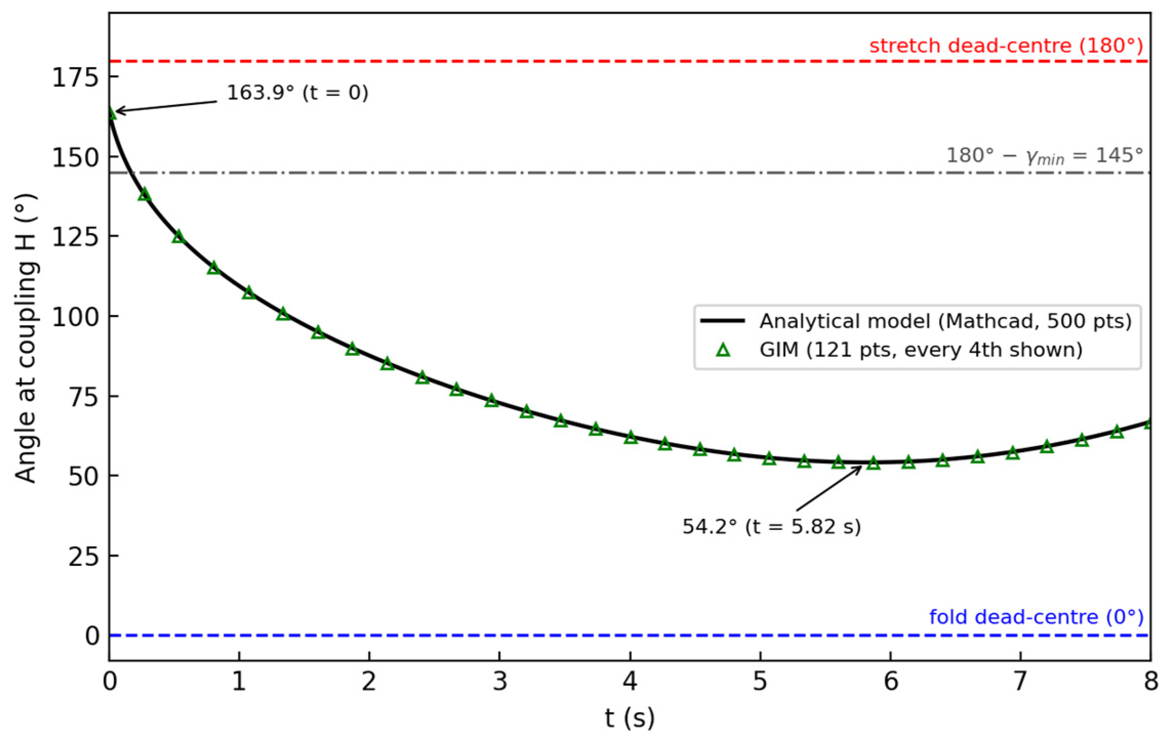
The configuration of the guiding dyad formed by the links GH and HI is governed by the distance d₂ between the fixed joint G and the mobile joint I (Equation (22)), the dyad reaching a stretch dead-centre at d₂ = g + h = 375 mm and a fold dead-centre at d₂ = ∣g − h∣ = 5 mm. Over the 500 computed positions of the extension stroke, d₂ decreases from a maximum of 371.30 mm at t = 0 to a single minimum of 170.80 mm at t = 5.82 s, ending at 206.85 mm.

The corresponding angle between GH and HI, evaluated at the joint H, decreases from 163.9° at the beginning of the stroke to a minimum of 54.2° at t = 5.82 s, ending at 66.9° as presented in Figure 9. Identical extreme values of d₂ were obtained from the GIM data set.

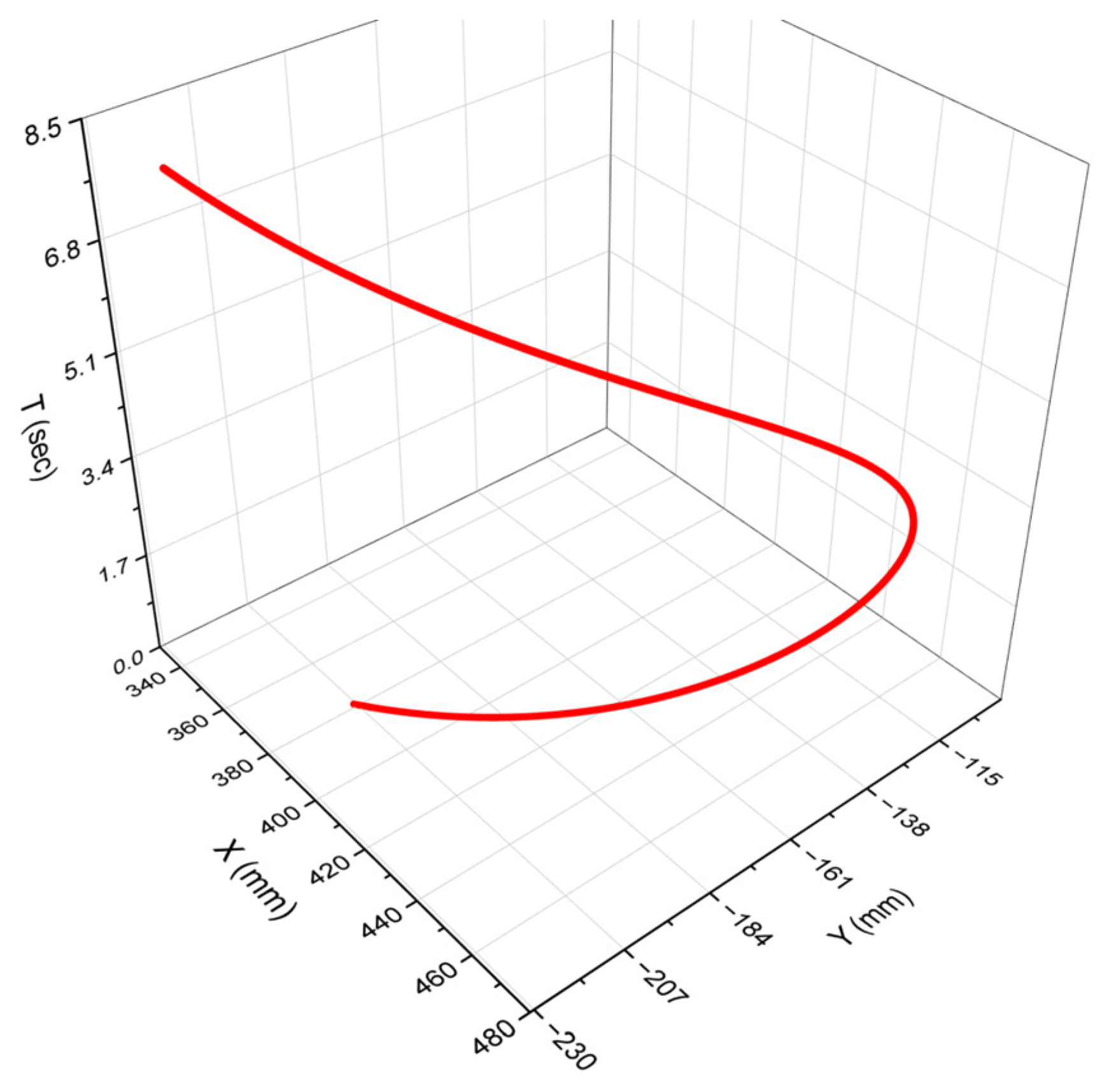
Figure 10 shows the three-dimensional trajectory of the joint H over time. From its initial position (x = 378.9 mm, y = −207.5 mm), the joint H executes an upward curvilinear movement in the XOY plane, followed after 3.04 s by a downward one. The input angle α is shown in Figure 11.

3.2. Results Obtained Through Simulation Software

The two dedicated packages introduced in Section 2, developed independently and based on distinct kinematic engines, were used for the cross-verification of the trajectories, GIM additionally supplying the velocities and the accelerations.

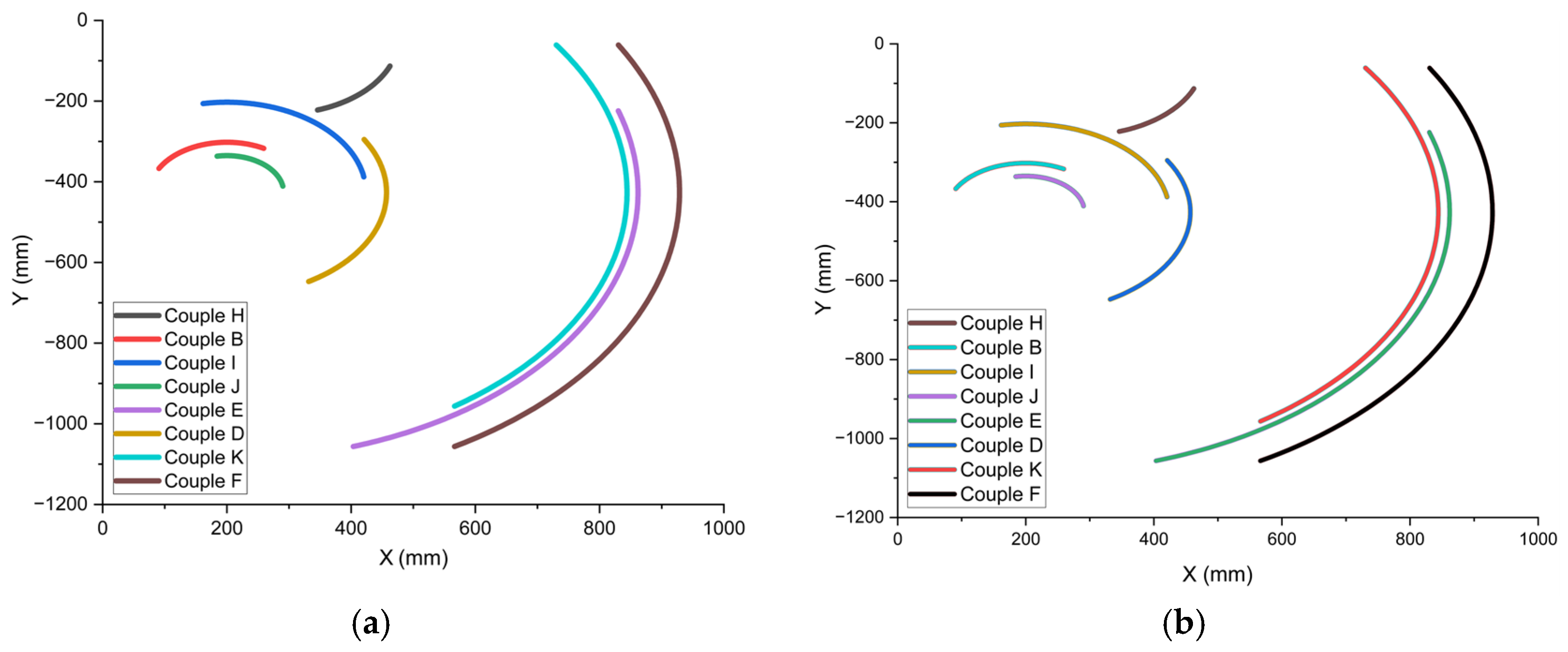
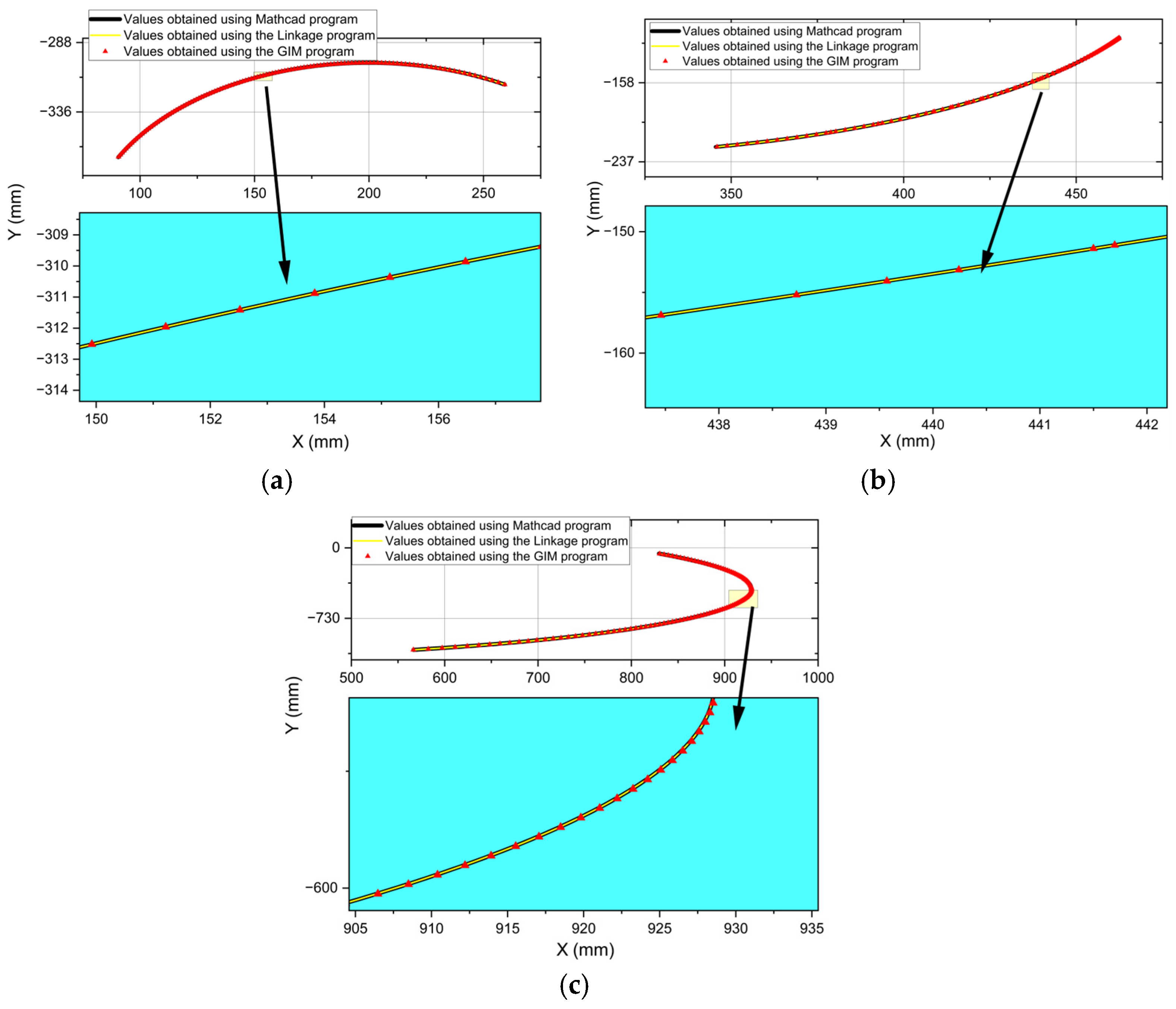
Figure 12 represents the trajectories corresponding to the analysed mobile joints, results obtained through both simulation software mentioned above.

Since Figure 7 and Figure 12 do not establish whether the trajectories are identical, three joints were selected for a quantitative comparison against both simulations: joint B, the connection between the actuator AB and the block, from which the motion is transmitted; joint H, whose trajectory is the most complex; and joint F, on the rigid block, closing the kinematic chain.

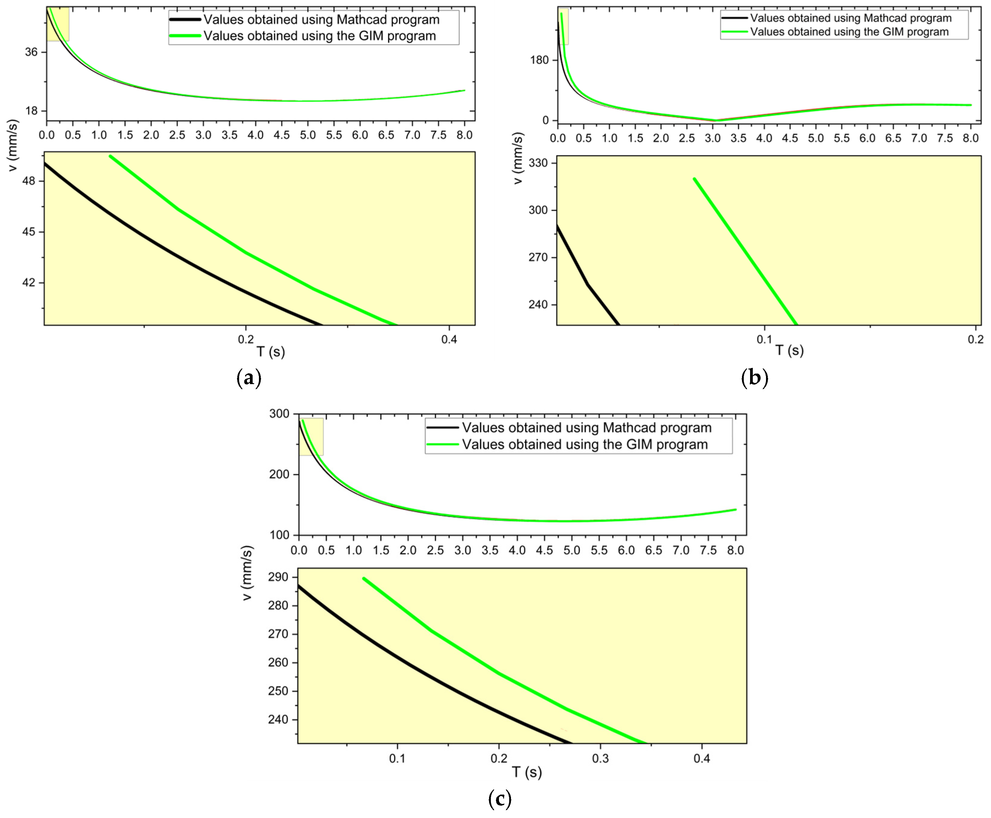
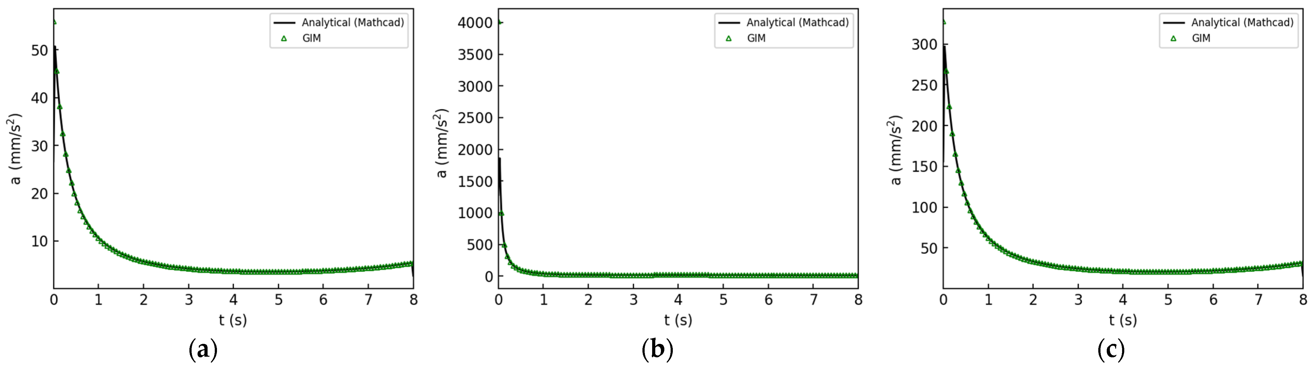
The deviations between the mathematical calculation and the two simulations were quantified for the positions, the velocities and the accelerations; the trajectories are compared against both environments, the velocities and accelerations against GIM alone, this being the only package returning them directly (Figure 13 and Figure 14).

Regardless of the method, the linear velocity decreases curvilinearly over 0–3 s and stabilises over 3–6 s, its variation being approximately 1.1 mm/s for joint B and 5.5 mm/s for joint F (Figure 14a,c).

In Figure 14c, the velocity of joint F passes through a minimum near zero at the reversal of joint H, after which it rises curvilinearly to a peak below the initial one.

The linear accelerations of the three joints, obtained as the second derivatives of the position equations and cross-verified against GIM (Figure 15), peak at the start of the stroke and decrease towards the end, the peak values being 56.1 mm/s² for joint B, 328.5 mm/s² for joint F and 4028.0 mm/s² for joint H, the last reflecting its more elaborate trajectory. The root-mean-square deviations are 0.021, 0.118 and 0.694 mm/s², respectively, and the mean deviations remain below 0.25% for all three joints (

Table 3. Deviations between the analytical model (Mathcad) and the GIM simulation.

Joint	Quantity	Unit	RMSE	${\mathit{e}}_{\mathit{m}\mathit{a}\mathit{x}}$	$\mathit{m}\mathit{a}\mathit{x} {\mathit{\epsilon }}_{\mathit{i}}$(%)	$\overline{{\mathit{\epsilon }}_{\mathit{i}}}$(%)	$\mathit{m}\mathit{a}\mathit{x} {\mathit{\epsilon }}_{\mathit{i}}^{\mathbf{\ast }}$(%)
B	position, X	mm	0.087	0.115	0.12	0.061	0.04
	position, Y	mm	0.081	0.197	0.05	0.017	0.05
	velocity	mm/s	0.029	0.056	0.21	0.116	0.11
	acceleration	mm/s2	0.021	0.125	0.49	0.230	0.22
H	position, X	mm	0.174	0.403	0.12	0.029	0.09
	position, Y	mm	0.129	0.225	0.13	0.062	0.10
	velocity	mm/s	0.080	0.318	15.96	0.570	0.10
	acceleration	mm/s2	0.694	7.528	0.25	0.160	0.19
F	position, X	mm	0.282	0.795	0.10	0.025	0.10
	position, Y	mm	0.754	1.196	2.00	0.269	0.11
	velocity	mm/s	0.154	0.292	0.19	0.104	0.10
	acceleration	mm/s2	0.118	0.694	0.48	0.218	0.21

Note: the error metrics of the velocity and of the acceleration are reported against the GIM output only, this being the sole environment among the two employed that returns these quantities directly; the trajectories are cross-verified against both environments.

).

3.3. Numerical Cross-Verification of the Analytical Model

Table 3 collects the deviations between the analytical model and GIM over the 120 samples for the joints B, H and F. The root-mean-square deviations of the coordinates remain below 0.18 mm for B and H and below 0.76 mm for F, over trajectory spans of order 10² mm for H and 10³ mm for F, and the velocity and acceleration deviations remain at the sub-millimetre-per-second and sub-millimetre-per-second-squared level.

At t = 3.067 s, one step after the reversal of joint H at t = 3.04 s, the analytical velocity is 0.365 mm/s and the absolute deviation 0.058 mm/s, so the local percentage error reaches 15.96%, whereas normalised by the velocity amplitude of 320.35 mm/s, it is only 0.02%; the maximum velocity deviation of this joint, 0.318 mm/s away from the reversal, is 0.10% of the amplitude. For the coordinates, the largest local error, 2.00%, occurs for y_F at the end of the stroke.

3.4. Admissible Design Domain of the Guiding Dyad

The distance d₂ between the fixed joint G and the mobile joint I, given by Equation (22), depends exclusively on the driving loop and on the rigid block and is therefore independent of the lengths g and h of the guiding dyad. The dyad is a passive follower whose input d₂ (t) is imposed from outside, and its singularity analysis consequently reduces to a one-dimensional problem in d₂. The admissible design domain of the pair (g, h) is then obtained in closed form, without any simulation: the condition that neither dead-centre be reached over the stroke is

$$g+h>\underset{t}{\max } d_2=371.30 \mathrm{m}\mathrm{m}$$

(34)

$$\left|g-h\right|<\underset{t}{\min } d_2=170.80 \mathrm{m}\mathrm{m}$$

(35)

while the condition that the transmission angle at the joint H remain above the minimum value γ_min = 35° adopted from [12] over the whole stroke is

$$g^2+h^2+2gh\cos {\gamma }_{min}\ge {\left(\underset{t}{\max } d_2\right)}^2$$

(36)

$$g^2+h^2-2gh\cos {\gamma }_{min}\le {\left(\underset{t}{\min } d_2\right)}^2$$

(37)

The sensitivity of the admissible domain to the adopted threshold γ_min follows from the same conditions. The fold-side conditions, Equations (35) and (37), remain satisfied with a wide margin for the geometries considered, so the binding boundary is the stretch-side condition, Equation (36); a larger γ_min displaces this boundary outward and contracts the admissible domain. Solving Equation (36) at equality, with the difference g − h held fixed, the minimum admissible span is obtained in closed form:

$${(g+h)}_{min}=\sqrt{{\displaystyle \frac{2d_{2,max}^2-{(g-h)}^2·\left(1-\cos {\gamma }_{min}\right)}{1+\cos {\gamma }_{min}}}}$$

(38)

For the difference g − h = 5.004 mm of the analysed pair, Equation (38) yields a minimum span of 384.40 mm at γ_min = 30° (g = 194.70 mm, h = 189.70 mm), of 389.31 mm at γ_min = 35° (g = 197.16 mm, h = 192.15 mm), and of 395.13 mm at γ_min = 40° (g = 200.07 mm, h = 195.06 mm), that is, increases of 2.51%, 3.82% and 5.37% over the analysed span of 375.00 mm. The maximum interior angle at H being 163.9°, the analysed pair delivers a transmission-angle margin of 16.1° at the stretch extreme and therefore fails all three thresholds; the value g = 197.16 mm, h = 192.15 mm is the boundary geometry for γ_min = 35° and remains admissible for any γ_min ≤ 35°, whereas a more conservative γ_min = 40° would require the larger span of 395.13 mm.

Although the analysed pair (g = 190.000 mm, h = 184.996 mm) therefore fails the 35° criterion, both dead-centres remain unattainable, the maximum d₂ of 371.30 mm lying 3.70 mm, or approximately 1%, below the stretch dead-centre of 375 mm, and the violation being confined to the first 0.176 s, that is, the first 2.2% of the stroke at the wheel-down configuration. The analysed pair is consequently a preliminary geometry, and the corrective pair g = 197.16 mm, h = 192.15 mm, which meets the criterion over the entire stroke while keeping both dead-centres unattainable, is recommended for the final dimensioning of the guiding dyad.

4. Discussion

The deviations of Table 3 are of numerical, not modelling, origin, attributable to the differing time steps and to the ill-conditioning of the local percentage error near the velocity reversal of joint H, as quantified in Section 3.3.

It should be noted that, in the absence of experimental measurements, the analytical and numerical approaches provide a mutual cross-verification rather than a formal validation in the strict sense. The close numerical agreement obtained is therefore interpreted as an indicator of the internal consistency of the proposed formulation, whereas its full experimental validation remains a subject for future work.

The kinematic stability of the proposed structure is confirmed by the analysis of angular variations. A linear increase with time is recorded for the dependent angles β, δ, ε, γ, τ and σ, which indicates a correct formulation of the geometric equations and emphasizes that the values obtained are generated by elements that are dependent on each other. In the case of this system, the variation in these angles is significantly influenced by the position of the fixed joint C, as well as by the value of the stroke executed by the hydraulic piston.

At the same time, a nonlinear variation is determined for the input parameter represented by the angle α, reflecting the variation in the hydraulic piston on the segment AB.

The angle υ has an asymmetric oscillatory variation, in which the increase phase is steeper than the decrease. This phenomenon indicates that the change in the angle over time is not uniform but influenced by the geometry and position of the moving elements.

The angle λ decreases monotonically along the whole stroke, from 102.98° in the extended configuration to −4.97° in the retracted one. In the original submission, this variation was reported in the interval 0–360°, which introduced an apparent discontinuity near the end of the stroke; the angles are now unwrapped, so the curve is continuous, and no numerical correction of the representation is required.

The identification of the wheel-down configuration as the critical design point, where the guiding dyad operates within 1% of its stretch dead-centre, makes the corrective pair g = 197.16 mm, h = 192.15 mm a functional requirement to preserve the transmission-angle margin during deployment.

Several limitations of the present study should be acknowledged in order to delimit the scope of the proposed model. First, the analysis is purely kinematic and rigid-body-based; the elastic deformations of the links and the compliance of the hydraulic actuator were neglected, all elements being treated as perfectly rigid. Second, the joint clearances at the fixed and mobile joints were not considered, although in practice they may introduce nonlinear behaviour and local deviations of the trajectories, as reported in the literature [26]. Third, the dynamic loads arising from impact at touchdown, as well as the aerodynamic forces acting during retraction, were not included in the current formulation, which addresses the motion transmission rather than the force distribution. Fourth, the extreme retracted and extended configurations were characterised only in terms of the planar kinematic behaviour of the mechanism, whereas the geometric clearance between the retracted landing gear and the surrounding fuselage structure was not verified; the confirmation of full retraction without interference requires the superposition of the swept envelope of the tyre and links onto the fuselage bay contour and is therefore reserved for the subsequent design stage together with the experimental and finite-element investigations.

Because physical-prototype calibration, joint clearance, hydraulic-oil elasticity and structural flexibility are not represented in the present rigid-body kinematic model, the reported conclusions are to be treated with caution when extrapolated to a full-scale aircraft.

These assumptions establish a rigorous baseline for the mechanism’s planar kinematics by separating the kinematic flow from elastic compliance and clearance effects. The resulting closed-form trajectories provide the input for future finite-element analysis and experimental studies addressing impact loads and fuselage-bay clearances. Future work will focus on designing an experimental stand to measure reaction forces at fixed joints A, C and G, complemented by finite-element analyses of induced stresses. This will support a predictive lifetime-assessment algorithm for aerospace assembly design.

5. Conclusions

This study establishes a closed-form kinematic model of a space-constrained retraction mechanism in which every mobile joint is expressed as an explicit function of the actuator length. The model is cross-verified against two independent packages, the deviations remaining below 0.25% of the amplitude of each quantity and the velocity root-mean-square deviations below 0.16 mm/s. The passive guiding dyad is characterised over the whole extension stroke, its governing distance d₂ varying between 371.30 mm and 170.80 mm, so that neither the stretch dead-centre at 375 mm nor the fold dead-centre at 5 mm is reached. The scientific contribution therefore consists of an original rigid-block topology with a dedicated out-of-plane restraint and of an explicit, simulation-free feasibility criterion for its guiding dyad, providing a quantified basis for the subsequent structural, dynamic and experimental analysis.

The distinctive feature is the guiding dyad GH–HI, which generates the non-monotonic trajectory of the joint H and supplies the out-of-plane restraint. The wheel-down configuration is identified as the critical design state, where the dyad operates near its stretch dead-centre, and the corrective pair g = 197.16 mm, h = 192.15 mm is required to meet the 35° transmission-angle margin.

The paper delivers an explicit, simulation-free feasibility criterion for the guiding dyad of this class of retraction mechanism, obtained by a closed-form parametric sweep of the (g, h) plane.

From an aeronautical perspective, the out-of-plane restraint furnished by the guiding links GH and HI confines the mechanism to the XOY plane at the kinematic level, providing the trajectory and velocity profiles required for the subsequent shock-absorption analysis, whereas the out-of-plane structural stiffness, the dynamic impact loads and the experimental validation on a laboratory stand are deferred to the finite-element stage.