Heterogeneous Graph Neural Network-Guided Adaptive Large Neighborhood Search for Flexible Job Shop Scheduling in Panel Furniture Production

Abstract

This study formulates panel furniture production as a flexible job shop scheduling problem (FJSP) with constraints on transport resources under varying production conditions. An adaptive large neighborhood search (ALNS) method guided by a heterogeneous graph neural network (HeteroGNN), termed HeteroGNN-ALNS, is developed to balance completion time, waiting time, and workload during the production process. The current scheduling state in ALNS is represented as a heterogeneous graph, where panel jobs and production resources are modeled as different node types, and assignment, transport, and sequence information is represented by different edge types. A search state vector is also introduced to describe the current search process. The HeteroGNN is trained using an actor–critic method to guide neighborhood operator selection and destroy set construction in ALNS. Experiments are conducted under four production conditions and five job scales. The results show that HeteroGNN-ALNS achieves better overall scheduling performance than dispatching rules and representative search methods. Statistical and ablation analyses further verify the effectiveness of the proposed method.

1. Introduction

Panel furniture production is a representative case of customized manufacturing. A customer order usually comprises a set of panels, which may differ in size, material, and process route [1]. Before assembly or packaging, each panel passes through several production stages, such as cutting, edge banding, drilling, and sorting [2]. In the practical production process, an operation may be processed by more than one available machine at each stage, and a panel may be transferred between stages through several feasible routes. Accordingly, the coordination of panel sequencing and machine assignment is central to improving production efficiency and meeting order delivery requirements.

This problem is commonly formulated as a flexible job shop scheduling problem (FJSP). The central decision is to determine machine assignment and processing sequence for a set of jobs under relevant process and resource constraints, with the aim of optimizing one or more performance criteria [3]. For example, Chen et al. and Moon et al. study FJSPs with transportation resource constraints [4,5]. The minimization of makespan and total energy consumption in an FJSP with uncertain processing times is considered in [6]. Lei et al. achieve real-time scheduling decisions for large-scale dynamic FJSP with random arrivals of new jobs [7].

The FJSP is an NP-hard problem, and metaheuristic algorithms are widely used to obtain solutions of high quality within a reasonable computational time [8]. Neighborhood search is a common idea in metaheuristics and improves a schedule by locally modifying the current solution [9]. However, for large-scale FJSPs with complex constraints, a single neighborhood or small local move is often insufficient to adjust the current solution structure effectively. Adaptive large neighborhood search (ALNS) extends neighborhood search by introducing a destroy-and-repair mechanism. It first removes part of the incumbent solution and then repairs the partial solution to explore a broader neighborhood. In addition, operator selection probabilities are adaptively updated according to search performance [10]. Liu et al. propose a multi-objective ALNS for dynamic FJSP with transportation resources to handle the coupled optimization of production and transportation decisions under new job insertion [11]. Kasapidis et al. propose a unified modeling framework and a constraint programming (CP)-based ALNS for FJSPs with constraints related to buffers, tools, and common resources [12].

However, the performance of ALNS is affected by neighborhood operator selection and destroy set construction. Traditional adaptive mechanisms update operator probabilities mainly from historical rewards [13]. Under a limited computational budget, this may lead to inefficient neighborhood searches and affect convergence speed and final solution quality. In recent studies, graph neural networks (GNNs) have been introduced to extract structural information from complex scenarios and to guide the solution process of the corresponding optimization methods. Teichteil-Königsbuch et al. study the resource-constrained project scheduling problem, where task starting-time information is learned from CP-generated schedules via GNNs and then guides a schedule generation scheme to construct feasible schedules [14]. Sui et al. propose NeuralGLS, which learns to guide local search with a graph convolutional network for the traveling salesman problem, thereby reducing ineffective moves and improving heuristic search performance [15]. The effectiveness of an ALNS operator is closely related to both the current solution structure and the search state. Local structural information from a static graph alone may be insufficient to represent the dynamic state of the ALNS search process. Johnn et al. formulate ALNS operator selection as a Markov decision process and combine deep reinforcement learning (DRL) with GNNs to select operators conditioned on the current solution state, which indicates that graph information can support operator control in ALNS [16]. Nevertheless, the search action in ALNS involves not only neighborhood operator selection but also the construction of the destroy set. Existing GNN-guided ALNS studies mainly focus on neighborhood operator selection, while relatively few studies use both solution structure and search state information to guide operator selection and destroy set construction simultaneously.

This paper proposes a heterogeneous graph neural network (HeteroGNN)-guided ALNS method, termed HeteroGNN-ALNS, for the scheduling problem in panel furniture production. Initially, the production process is formulated as an FJSP with multiple constraints. ALNS is adopted to solve this FJSP, and the current scheduling state is represented as a heterogeneous graph. HeteroGNN is then used to extract structural features from jobs, resources, and transport relations. In addition, graph embeddings are combined with the search state vector to support both operator decision and destroy decision in ALNS. Finally, the proposed method is evaluated on instances of different job scales and under four production conditions, namely normal production, machine breakdown, job cancellation, and topology change.

The main contributions of this paper are summarized as follows.

• An FJSP model is formulated to represent the practical production process of panel furniture. The model considers multiple scheduling objectives under different processing times, variable transport resources, and specific production constraints.
• A heterogeneous graph representation is developed to describe the scheduling state in ALNS. Panel jobs and production resources at different stages are represented as different node types, while assignment, transport, and sequence information is represented by different edge types. A search state vector describing the current ALNS search process is further combined with the graph representation as input to the HeteroGNN to capture both the scheduling structure and the current search state.
• A HeteroGNN-guided ALNS method is developed to guide neighborhood operator selection and destroy set construction according to the current scheduling and search states. The guidance policy is trained using an actor–critic method and is periodically incorporated into the adaptive search process of ALNS.

2. Related Work

2.1. ALNS for FJSP

Conventional heuristic methods for complex FJSP instances tend to rely on limited neighborhood exploration, which makes them prone to premature convergence to local optima [17]. Large neighborhood search (LNS) is a heuristic framework designed for complex combinatorial optimization problems. It explores a broader search space by destroying part of the current solution and repairing it into a feasible solution, which helps the search escape local optima and identify better candidate solutions [18]. ALNS extends this framework by evaluating the effects of different destroy and repair operators during the search and adjusting their selection probabilities accordingly [19]. This mechanism allows the algorithm to favor more effective operators when modifying the current solution, thereby increasing the chance of finding higher-quality solutions [20].

Existing studies focus on joint machine selection and operation sequencing in FJSP with multiple resources and process constraints. For example, Liu et al. embed a feasibility correction strategy and a variable neighborhood search with self-learning into a genetic algorithm for FJSP with machine and auxiliary resource constraints [21]. Yunusoglu et al. combine CP and LNS to solve an FJSP batch flow problem with setup times and transportation resource constraints [22]. Ji et al. study a large-scale FJSP with batch-processing machines, formulate the problem as a multicommodity flow model, and propose an improved ALNS framework with optimization-based repair and tabu components [23]. Wang et al. address FJSP with preventive maintenance under frequent production changeovers by formulating a two-stage joint optimization model and designing a hybrid metaheuristic algorithm to coordinate machine assignment, operation sequencing, and maintenance scheduling [24].

The performance of ALNS is affected by neighborhood structure design and adaptive operator selection, particularly in FJSP with multiple constraints [25]. Learning-based adaptive strategies have been introduced into metaheuristic search in recent studies. Reijnen et al. apply DRL to ALNS so that operator selection, parameter configuration, and acceptance criteria can be adjusted according to the search state [26]. Wang et al. propose proximal policy optimization-guided ALNS for the vehicle routing problem with time windows, where reinforcement learning supports adaptive decision-making in ALNS [27]. Qin et al. develop a reinforcement-learning-enhanced quality-diversity algorithm for FJSP with transportation constraints, in which Q-learning is used to select search regions and maintain solution diversity [28].

Overall, the reviewed studies indicate that neighborhood design and adaptive search decisions have an important effect on the effectiveness of ALNS. Accordingly, the following subsection discusses GNNs for learning structured representations of scheduling states to improve ALNS performance.

2.2. GNNs for Scheduling

GNNs are a class of deep neural networks for learning representations of graph-structured data. In a typical GNN, node representations are updated through neighborhood aggregation, where graph topology and node features determine the information passed among nodes [29]. This graph representation allows operation and machine features to be learned, and candidate operation–machine pairs are evaluated for joint operation selection and machine assignment thereafter [30,31]. With respect to more complex production scenarios, HeteroGNN models are increasingly used to model shop-floor states that contain different types of objects and relations [32]. A heterogeneous graph representation of the current scheduling state is presented in [33], where a HeteroGNN captures complex relationships among operations and machines to support dynamic scheduling decisions. A meta-path-based HeteroGNN is introduced in [34], which models different semantic associations in FJSP graphs and learns scheduling state representations from specific relation paths. For multivariety and variable-batch production environments, a heterogeneity-enhanced incidence graph is developed in [35], which extends heterogeneous graph modeling to more complex flexible job shop scheduling states.

Graph learning and related learning policies have also been incorporated into improvement-based search, where learned signals guide neighborhood construction, move evaluation, or local adjustment around an incumbent solution. For example, Wu et al. introduce a learned destroy operator into LNS, where the policy selects a subset of variables for reoptimization [36]. Hudson et al. combine GNNs with guided local search (GLS), where the model predicts the regret of including each edge of the problem graph in the solution and GLS searches with these predictions in conjunction with the original problem graph [37]. Zhang et al. propose a topology-aware bidirectional graph attention network, which embeds the disjunctive graph of a job shop scheduling problem into a local search framework and learns topological representations of scheduling solutions from both forward and backward views [38]. Wang et al. propose a memory-enhanced improvement search framework for FJSP, where a complete schedule is represented by a heterogeneous disjunctive graph and state features are extracted by a memory-enhanced HeteroGNN to guide local move selection and neighborhood improvement [39].

3. Problem Formulation

3.1. Problem Description

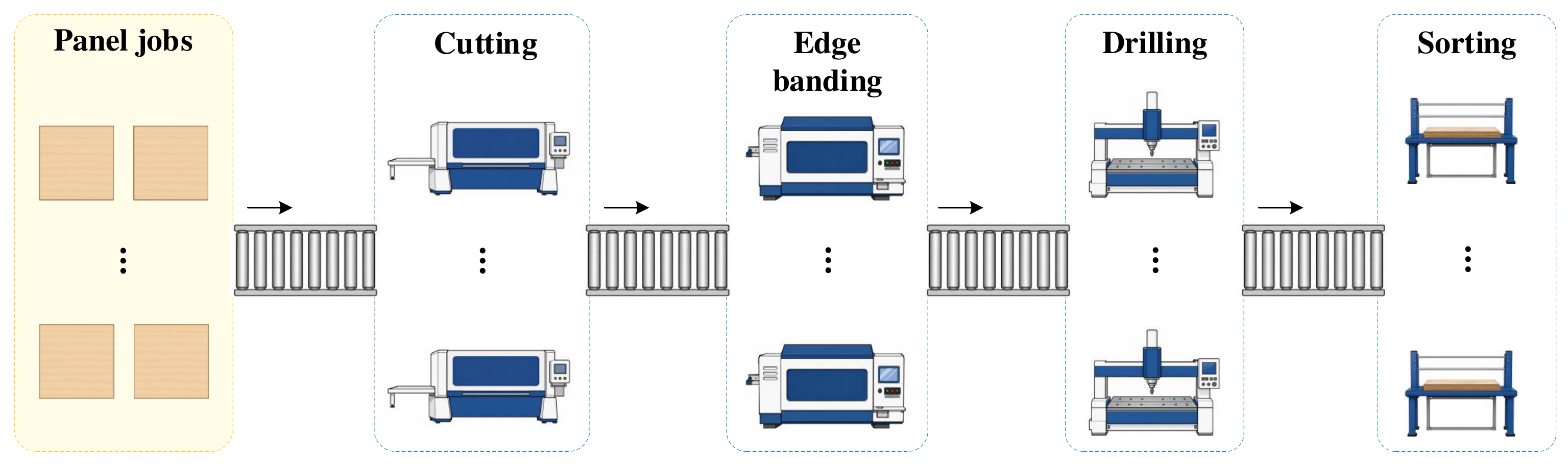
An FJSP in panel furniture production is considered in this paper. In the considered production system, customer orders are decomposed into a set of panel jobs. These panel jobs pass through four production stages in sequence, namely cutting, edge banding, drilling, and sorting, with different available machines at each stage. In addition, panels are transported between adjacent stages through roller conveyors. The production process is illustrated in Figure 1.

Compared with a standard FJSP, several additional constraints are considered in this problem. Firstly, the dimensions of panels may vary across jobs, and the processing time of each job is determined by its dimensions and process requirements. Furthermore, a minimum safety time interval is maintained between two consecutive panels to prevent collisions during the edge banding stage, and this interval is also related to the size of panel jobs. Accordingly, a panel transported from the cutting stage may wait before edge banding until the preceding panel satisfies the required minimum safety time interval. In addition, transport connectivity may change in practical production environments.

Remark 1.

In practical production, panels are generally transported at a constant speed on roller conveyors. Except when congestion occurs at downstream stages, panels generally do not collide during processing or transport. In particular, the edge banding stage comprises four sequential processing units and a turning mechanism located between the second and third units. At this stage, the two long edges of each panel are processed first, after which the panel is rotated by 90° and the two short edges are processed in sequence. The rotation requires a minimum safety distance between consecutive panels. Since the roller conveyors operate at a constant speed, the minimum safety distance is represented in the mathematical model by a minimum safety time interval before the next panel enters the edge banding stage.

The formulation is based on the following assumptions.

• All panel jobs are available at the beginning of the planning horizon.
• Each job is processed once at each required stage and follows the stage order of cutting, edge banding, drilling, and sorting.
• At each stage, each job is assigned to one available resource, and transport between two consecutive stages is permitted only between resources with a feasible transport connection.
• Each processing resource in cutting, drilling, and sorting handles at most one job at a time. A job may start before the preceding job is completed at the edge banding stage, provided that the minimum safety time interval is satisfied.
• Processing operations cannot be interrupted once they have started.
• At least one resource is available at each production stage.

For clarity,

Table 1. Main notation.

Symbol	Description
$\mathcal{J}$	Set of panel jobs, where $\mathcal{J}=\{1,2,\dots ,J\}$ and $j\in \mathcal{J}$.
$\mathcal{L}$	Set of production stages, where $\mathcal{L}=\{c,b,d,s\}$ denotes cutting, edge banding, drilling, and sorting, respectively.
$\mathcal{A}$	Set of ordered pairs of adjacent production stages, where $\mathcal{A}=\left\{\right(c,b),(b,d),(d,s\left)\right\}$.
$(o^{\prime },o)$	$o^{\prime }$ denotes the stage immediately preceding the downstream stage o for $(o^{\prime },o)\in \mathcal{A}$.
${\mathcal{R}}_o$	Set of resources at stage o.
${\mathcal{E}}^{o^{\prime },o}$	Set of feasible transport connections from stage $o^{\prime }$ to stage o, where $(o^{\prime },o)\in \mathcal{A}$.
${\tau }_{r^{\prime }r}^{o^{\prime },o}$	Transport time from resource $r^{\prime }\in {\mathcal{R}}_{o^{\prime }}$ to resource $r\in {\mathcal{R}}_o$, where $(o^{\prime },o)\in \mathcal{A}$.
$h_j$	Minimum safety time interval for job j at the edge banding stage.
$a_r^o$	1 if resource r at stage o is available and 0 otherwise.
$x_{jr}^o$	1 if job j is assigned to resource r at stage o and 0 otherwise.
$y_{j{r}^{\prime }r}^{o^{\prime },o}$	1 if the transport connection from resource $r^{\prime }$ at stage $o^{\prime }$ to resource r at stage o is selected for job j and 0 otherwise.
$z_{ij}^o$	Binary sequencing variable, where $z_{ij}^o\in \{0,1\}$. $z_{ij}^o=1$ if job i precedes job j at stage o for $i,j\in \mathcal{J}$ and $i<j$, and $z_{ij}^o=0$ otherwise.
$A_j^o$	Arrival time of job j at stage o.
$S_j^o$	Start time of job j at stage o.
$C_j^o$	Completion time of job j at stage o.
$W_j^o$	Waiting time of job j at stage o.
$B_r^o$	Workload of resource r at stage o.

presents the main notation adopted in the mathematical model.

3.2. Variable Definitions

The completion time at each production stage is written as

$$C_j^o=S_j^o+\sum _{r\in {\mathcal{R}}_o}{p}_{jr}^o{x}_{jr}^o,\forall j\in \mathcal{J},o\in \mathcal{L},$$

(1)

where $p_{jr}^o$ denotes the processing time of job j on resource r at stage o.

For downstream stages, the arrival time can be expressed as

$$A_j^o=C_j^{o^{\prime }}+\sum _{(r^{\prime },r)\in {\mathcal{E}}^{o^{\prime },o}}{\tau }_{r^{\prime }r}^{o^{\prime },o}{y}_{j{r}^{\prime }r}^{o^{\prime },o},\forall j\in \mathcal{J},(o^{\prime },o)\in \mathcal{A}.$$

(2)

The waiting time at each downstream stage is given by

$$W_j^o=S_j^o-A_j^o,\forall j\in \mathcal{J},o\in \{b,d,s\}.$$

(3)

The processing workload assigned to each resource is calculated as

$$B_r^o=\sum _{j\in \mathcal{J}}{p}_{jr}^o{x}_{jr}^o,\forall o\in \mathcal{L},r\in {\mathcal{R}}_o.$$

(4)

3.3. Objective Function

Completion time is an important criterion for the FJSP in panel furniture production. Since transport times between adjacent stages depend on the selected resources, minimizing completion time alone may repeatedly favor shorter transport routes and result in increased waiting time and workload imbalance. Therefore, average completion time is considered together with average waiting time and workload imbalance in the objective function.

The average completion time and the average waiting time are defined as

$$\begin{array}{cc}\hfill C_{\mathrm{avg}}& ={\displaystyle \frac{1}{J}}\sum _{j\in \mathcal{J}}{C}_j^s,\hfill \\ \hfill W_{\mathrm{avg}}& ={\displaystyle \frac{1}{J}}\sum _{j\in \mathcal{J}}\sum _{o\in \{b,d,s\}}{W}_j^o.\hfill \end{array}$$

(5)

Let $N_o={\sum }_{r\in {\mathcal{R}}_o}{a}_r^o$ denote the number of available resources at stage o, and let ${\overline{B}}^o={\displaystyle \frac{1}{N_o}}{\sum }_{r\in {\mathcal{R}}_o}{a}_r^o{B}_r^o$. According to Assumption 6, $N_o>0$.

The workload imbalance is measured by the total absolute deviation of the workload assigned to each resource from the average workload at the corresponding production stage, which is given by

$$I_{\mathrm{load}}=\sum _{o\in \mathcal{L}}\sum _{r\in {\mathcal{R}}_o}{a}_r^o\left|B_r^o-{\overline{B}}^o\right|.$$

(6)

The objective function is formulated as

$$\min F=w_C{C}_{\mathrm{avg}}+w_W{W}_{\mathrm{avg}}+w_L{I}_{\mathrm{load}}.$$

(7)

Here, $w_C$, $w_W$, and $w_L$ are non-negative weights.

3.4. Constraints

The resource assignment constraint specifies that exactly one eligible resource is selected for each job at each production stage, which is written as

$$\sum _{r\in {\mathcal{R}}_o}{x}_{jr}^o=1,\forall j\in \mathcal{J},o\in \mathcal{L}.$$

(8)

The assignment to an unavailable resource is prevented by

$$x_{jr}^o\le a_r^o,\forall j\in \mathcal{J},o\in \mathcal{L},r\in {\mathcal{R}}_o.$$

(9)

Specifically, $a_r^d=0$ is specified to prohibit job assignment to an unavailable resource under machine breakdown.

Since the transport time depends on the resources selected at adjacent stages, the transport variable is constrained as follows.

$$y_{j{r}^{\prime }r}^{o^{\prime },o}\le x_{j{r}^{\prime }}^{o^{\prime }},\forall j\in \mathcal{J},(o^{\prime },o)\in \mathcal{A},(r^{\prime },r)\in {\mathcal{E}}^{o^{\prime },o}.$$

(10)

$$y_{j{r}^{\prime }r}^{o^{\prime },o}\le x_{jr}^o,\forall j\in \mathcal{J},(o^{\prime },o)\in \mathcal{A},(r^{\prime },r)\in {\mathcal{E}}^{o^{\prime },o}.$$

(11)

$$y_{j{r}^{\prime }r}^{o^{\prime },o}\ge x_{j{r}^{\prime }}^{o^{\prime }}+x_{jr}^o-1,\forall j\in \mathcal{J},(o^{\prime },o)\in \mathcal{A},(r^{\prime },r)\in {\mathcal{E}}^{o^{\prime },o}.$$

(12)

Exactly one feasible transport connection is selected for each job between two adjacent stages as

$$\sum _{(r^{\prime },r)\in {\mathcal{E}}^{o^{\prime },o}}{y}_{j{r}^{\prime }r}^{o^{\prime },o}=1,\forall j\in \mathcal{J},(o^{\prime },o)\in \mathcal{A}.$$

(13)

In addition to assignment and transport constraints, several standard FJSP constraints are imposed in this paper.

The start time restrictions are given by

$$S_j^c\ge 0,S_j^o\ge A_j^o,\forall j\in \mathcal{J},o\in \{b,d,s\}.$$

(14)

Particularly, the start times at the edge banding stage are constrained by the minimum safety time interval between jobs as

$$\begin{array}{cc}\hfill S_j^b& \ge S_i^b+h_i-M(1-z_{ij}^b),\hfill \\ \hfill S_i^b& \ge S_j^b+h_j-M{z}_{ij}^b,\hfill \end{array}\forall i,j\in \mathcal{J},i<j,$$

(15)

where M denotes a sufficiently large positive constant.

The resource capacity constraints for any two jobs assigned to the same resource at the cutting, drilling, or sorting stage are formulated as

$$\begin{array}{cc}\hfill C_i^o& \le S_j^o+M\left(3-x_{ir}^o-x_{jr}^o-z_{ij}^o\right),\hfill \\ \hfill C_j^o& \le S_i^o+M\left(2-x_{ir}^o-x_{jr}^o+z_{ij}^o\right),\hfill \end{array}\forall i,j\in \mathcal{J},i<j,o\in \{c,d,s\},r\in {\mathcal{R}}_o.$$

(16)

4. HeteroGNN-Guided ALNS

4.1. Solution Representation in ALNS

At iteration t, the encoded solution maintained by ALNS is represented as a job sequence

$$s_t={\pi }_t=({\pi }_t\left(1\right),{\pi }_t\left(2\right),\dots ,{\pi }_t\left(J\right)),$$

(17)

where ${\pi }_t$ is a permutation of all panel jobs, and ${\pi }_t\left(q\right)$ denotes the job at the q-th position in the sequence.

The encoded solution is decoded according to the job order in ${\pi }_t$. For each job, feasible resource assignments are generated, and the resulting feasible alternatives are ranked lexicographically according to the current makespan, cumulative downstream waiting time, $C_j^s$, $C_j^d$, and transport time. The alternative ranked first is selected for the initial schedule, whereas one alternative from the first $K_R$ alternatives is uniformly selected during the search. The decoding procedure is summarized in Algorithm 1.

Algorithm 1 Schedule decoding

1: function Decode($s,K$)   2:     Initialize an empty schedule $\sigma$   3:     for $q=1,2,\dots ,J$ do   4:         Set $j\leftarrow \pi \left(q\right)$   5:         Enumerate feasible resource assignments for job j subject to Equations (8)–(13)   6:         for each feasible resource assignment do   7:            Determine $A_j^o$, $S_j^o$, $C_j^o$, and $W_j^o$ according to Equations (1)–(3) and (14)–(16)   8:         end for   9:         Rank the feasible alternatives according to the lexicographic criterion defined above 10:         Uniformly select one alternative from the first K alternatives 11:         Assign the selected alternative to job j and update $\sigma$ 12:     end for 13:     return $\sigma$ 14: end function

To account for differences in scale among the three criteria, min–max normalization is applied before solution evaluation. Let $f_C\left(\sigma \right)=C_{\mathrm{avg}}\left(\sigma \right)$, $f_W\left(\sigma \right)=W_{\mathrm{avg}}\left(\sigma \right)$, and $f_L\left(\sigma \right)=I_{\mathrm{load}}\left(\sigma \right)$. For each criterion $k\in \{C,W,L\}$, the lower and upper bounds are obtained from a set of reference schedules ${\mathcal{S}}^{\mathrm{ref}}$ as

$$f_k^{\min }=\underset{\sigma \in {\mathcal{S}}^{\mathrm{ref}}}{\min }{f}_k\left(\sigma \right),f_k^{\max }=\underset{\sigma \in {\mathcal{S}}^{\mathrm{ref}}}{\max }{f}_k\left(\sigma \right),k\in \{C,W,L\}.$$

(18)

The normalization bounds are calculated before the search and remain fixed throughout the search. Accordingly, the normalized value of criterion k is calculated by

$${\tilde{f}}_k\left(\sigma \right)={\displaystyle \frac{f_k\left(\sigma \right)-f_k^{\min }}{f_k^{\max }-f_k^{\min }}},k\in \{C,W,L\}.$$

(19)

The normalized scalar objective is then given by

$$F^{\mathrm{norm}}\left(\sigma \right)=\sum _{k\in \{C,W,L\}}{\omega }_k{\tilde{f}}_k\left(\sigma \right),$$

(20)

where ${\omega }_k$ denotes the weight of criterion k.

4.2. Architecture of the HeteroGNN

The decoded schedule ${\sigma }_t$ is represented as a heterogeneous graph when the HeteroGNN is invoked. The graph representation is given by

$${\mathcal{G}}_t=({\mathcal{V}}_t,{\mathcal{E}}_t,{\mathbf{X}}_t),$$

(21)

where ${\mathcal{V}}_t$ and ${\mathcal{E}}_t$ denote the node and edge sets, respectively, and ${\mathbf{X}}_t$ contains the node feature matrices.

The set of node types is given by

$${\mathcal{T}}_V=\{\mathrm{j},\mathrm{c},\mathrm{b},\mathrm{d},\mathrm{s}\},$$

(22)

where $\mathrm{j}$ denotes the job node type, while $\mathrm{c}$, $\mathrm{b}$, $\mathrm{d}$, and $\mathrm{s}$ denote the resource node types corresponding to the four production stages defined in Section 3. The type of a node $v\in {\mathcal{V}}_t$ is denoted by $\varphi \left(v\right)\in {\mathcal{T}}_V$.

The corresponding node set is expressed as

$${\mathcal{V}}_t={\mathcal{V}}_t^{\mathrm{j}}\cup {\mathcal{V}}_t^{\mathrm{c}}\cup {\mathcal{V}}_t^{\mathrm{b}}\cup {\mathcal{V}}_t^{\mathrm{d}}\cup {\mathcal{V}}_t^{\mathrm{s}},$$

(23)

where ${\mathcal{V}}_t^{\mathrm{j}}$ denotes the set of job nodes, and ${\mathcal{V}}_t^o$ denotes the set of resource nodes at stage $o\in \mathcal{L}$.

Each node is associated with a feature vector describing the corresponding job or resource state. The static and dynamic features of the different node types are summarized in

Table 2. Node features.

Node Type	Static Features	Dynamic Features	Input Dimension
Job	Processing times, minimum safety time interval, panel length	Sorting completion time, downstream waiting time, sequence position, residual time, bottleneck ratio, waiting ratio, urgency	12
Cutting resource	Transport time to edge banding, resource index	Assigned-job ratio, utilization	4
Edge banding resource	Resource index	Assigned-job ratio, average waiting time, utilization	4
Drilling resource	Transport time from edge banding, reachability ratio, resource index	Assigned-job ratio, queue ratio, average waiting time	6
Sorting resource	Resource index	Assigned-job ratio, queue ratio, average waiting time	4

, and the input features are normalized before being fed into the network.

Different edge types are introduced to represent the relations in the current scheduling state. For an edge $e\in {\mathcal{E}}_t$, its type is denoted by $\tau \left(e\right)\in {\mathcal{T}}_E$, where ${\mathcal{T}}_E$ is the set of edge types. The graph contains assignment, transport, and sequence relations. Assignment edges connect each job to the resources assigned to it in the decoded schedule. Transport edges represent feasible connections between resources at adjacent production stages according to ${\mathcal{E}}^{o^{\prime },o}$ defined in Section 3. Sequence edges connect adjacent jobs in the current job sequence. Reverse edges are included to allow bidirectional message passing.

To provide dynamic search information for learning the operator selection policy, a search state vector $z_t$ is provided to the HeteroGNN together with the graph representation ${\mathcal{G}}_t$. Considering four types of signals relevant to adaptive decision-making in ALNS, including the annealing status, search effectiveness, stagnation, and exploration behavior, the search state vector is given by

$${\mathbf{z}}_t=[{\eta }_t,T_t,{\alpha }_t,{\beta }_t,{\xi }_t,1-{\eta }_t,{\zeta }_t,{\nu }_t],$$

(24)

where ${\eta }_t=t/I_{\max }$ and $1-{\eta }_t$ denote the elapsed and remaining proportions of the search budget, respectively. $I_{\max }$ is the maximum number of iterations. Both proportions characterize the current search progress. The variable $T_t$ denotes the current simulated annealing (SA) temperature, which determines the acceptance probability of a worse candidate schedule during the search. The variables ${\alpha }_t$, ${\beta }_t$, and ${\nu }_t$ denote the acceptance rate, the improvement rate of the best schedule, and the acceptance rate of worse schedules over the most recent search iterations, respectively. Search stagnation is represented by ${\xi }_t=\min \{u_t/I_{\max },1\}$, where $u_t$ is the number of iterations since the last improvement of the best schedule. The relative difference between the current schedule and the best schedule is given by

$${\zeta }_t={\displaystyle \frac{F^{\mathrm{norm}}\left({\sigma }_t\right)-F^{\mathrm{norm}}\left({\sigma }_t^{*}\right)}{\left|F^{\mathrm{norm}}\left({\sigma }_t^{*}\right)\right|+ϵ}},$$

(25)

where $ϵ$ is a small positive constant.

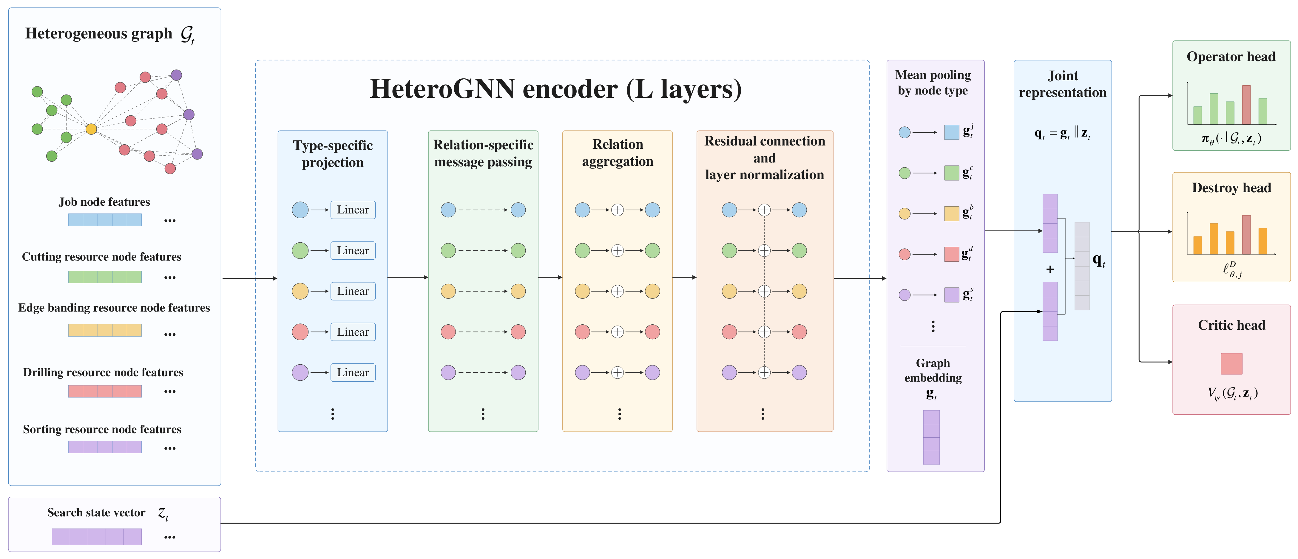
The architecture of the HeteroGNN is illustrated in Figure 2.

The input dimensions differ among node types. The input feature vector of each node is projected into a common hidden space of dimension $d_h$ by a type-specific linear transformation followed by a rectified linear unit (ReLU). The initial representation of node v is obtained as

$${\mathbf{h}}_v^{\left(0\right)}=\mathrm{ReLU}\left({\mathbf{W}}_{\varphi \left(v\right)}{\mathbf{x}}_v+{\mathbf{b}}_{\varphi \left(v\right)}\right),$$

(26)

where ${\mathbf{x}}_v$ denotes the input feature vector of node v. ${\mathbf{W}}_{\varphi \left(v\right)}\in {\mathbb{R}}^{d_h\times d_{\varphi \left(v\right)}}$ is the learnable projection matrix, where $d_{\varphi \left(v\right)}$ denotes the input dimension of node type $\varphi \left(v\right)$. The hidden dimension is set to $d_h=64$ in this study. ${\mathbf{b}}_{\varphi \left(v\right)}\in {\mathbb{R}}^{d_h}$ is the corresponding bias vector.

Information is subsequently propagated according to the different edge types. For an edge type $\kappa \in {\mathcal{T}}_E$, the neighbors of node v connected through relation $\kappa$ are denoted by ${\mathcal{N}}_{\kappa }\left(v\right)$.

At layer ℓ, the message associated with relation $\kappa$ is obtained by mean aggregation as

$${\mathbf{m}}_{v,\kappa }^{\left(\mathcal{l}\right)}=\mathrm{MEAN}\left(\left\{{\mathbf{h}}_u^{(\mathcal{l}-1)}\mid u\in {\mathcal{N}}_{\kappa }\left(v\right)\right\}\right).$$

(27)

The messages obtained from the different relations are then combined with the representation of node v. Its representation at layer ℓ is updated as

$${\mathbf{h}}_v^{\left(\mathcal{l}\right)}=\mathrm{LayerNorm}\left[\mathrm{ReLU}\left({\mathbf{h}}_v^{(\mathcal{l}-1)}+\sum _{\kappa \in {\mathcal{T}}_E\left(v\right)}{\mathbf{W}}_{\kappa }^{\left(\mathcal{l}\right)}\left[{\mathbf{h}}_v^{(\mathcal{l}-1)}\parallel {\mathbf{m}}_{v,\kappa }^{\left(\mathcal{l}\right)}\right]\right)\right],$$

(28)

where ${\mathcal{T}}_E\left(v\right)$ denotes the set of edge types incident to node v, ${\mathbf{W}}_{\kappa }^{\left(\mathcal{l}\right)}$ is the transformation matrix associated with relation $\kappa$, and ‖ denotes vector concatenation.

After L message-passing layers, mean pooling is applied separately to each node group. The corresponding pooled representations are computed as

$${\mathbf{g}}_t^{\mathrm{j}}={\displaystyle \frac{1}{|{\mathcal{V}}_t^{\mathrm{j}}|}}\sum _{v\in {\mathcal{V}}_t^{\mathrm{j}}}{\mathbf{h}}_v^{\left(L\right)},{\mathbf{g}}_t^o={\displaystyle \frac{1}{|{\mathcal{V}}_t^o|}}\sum _{v\in {\mathcal{V}}_t^o}{\mathbf{h}}_v^{\left(L\right)},o\in \mathcal{L}.$$

(29)

The pooled representations of the node groups are concatenated to obtain the graph embedding. The resulting graph embedding is expressed as

$${\mathbf{g}}_t={\mathbf{g}}_t^{\mathrm{j}}\parallel {\mathbf{g}}_t^{\mathrm{c}}\parallel {\mathbf{g}}_t^{\mathrm{b}}\parallel {\mathbf{g}}_t^{\mathrm{d}}\parallel {\mathbf{g}}_t^{\mathrm{s}}.$$

(30)

The graph embedding is further combined with the search state vector. The resulting representation is given by

$${\mathbf{q}}_t={\mathbf{g}}_t\parallel {\mathbf{z}}_t.$$

(31)

Three outputs are produced by the HeteroGNN based on ${\mathbf{q}}_t$. The probability distribution over the sequence neighborhood operators obtained from the operator head is given by

$${\mathit{\pi }}_{\theta }(·\mid {\mathcal{G}}_t,{\mathbf{z}}_t)=\mathrm{softmax}\left(f_{\pi }\left({\mathbf{q}}_t\right)\right).$$

(32)

The score assigned to each job by the destroy head is computed as

$${\mathcal{l}}_{\theta ,j}^D=f_D\left({\mathbf{h}}_{v_j}^{\left(L\right)}\parallel {\mathbf{q}}_t\right),j\in \mathcal{J},$$

(33)

where $v_j$ denotes the node corresponding to job j.

The value of the current state estimated by the critic head is given by

$$V_{\psi }({\mathcal{G}}_t,{\mathbf{z}}_t)=f_V\left({\mathbf{q}}_t\right).$$

(34)

Here, $f_{\pi }$, $f_D$, and $f_V$ denote the operator, destroy, and value heads, respectively.

4.3. Generation of Neighborhood Solutions

Let $\mathsf{\Omega }$ denote the set of operators used in the search. Four operators acting on the job sequence are included. The block relocation operator removes a consecutive block of jobs and reinserts it at another position. The subset shuffling operator rearranges the jobs in a selected subset. The block reversal operator reverses the order of jobs within a consecutive block. The $h_j$ interval operator selects jobs from the lower and upper ranges of the minimum safety time interval $h_j$ and rearranges them in the sequence.

The operator $a_t$ is sampled from the operator policy in training according to

$$a_t\sim \mathrm{Categorical}\left({\mathit{\pi }}_{\theta }(·\mid {\mathcal{G}}_t,{\mathbf{z}}_t)\right).$$

(35)

The operator with the highest probability is selected for inference as

$$a_t=\arg \underset{a\in \mathsf{\Omega }}{\max }{\mathit{\pi }}_{\theta }(a\mid {\mathcal{G}}_t,{\mathbf{z}}_t).$$

(36)

The number of jobs removed from the current sequence is controlled by the destroy ratio. The destroy size at iteration t is calculated as

$$n_t^D=\min \left\{J,\max \{n_{\min }^D,\lfloor {\lambda }_{D}J\rfloor \}\right\},$$

(37)

where $n_{\min }^D$ denotes the minimum destroy size and ${\lambda }_D$ denotes the destroy ratio.

The destroy scores produced by the destroy head are converted into a probability distribution for job selection. The probability associated with job j is given by

$${\mu }_{t,j}={\displaystyle \frac{\exp ({\mathcal{l}}_{\theta ,j}^D/T_D)}{{\sum }_{i\in \mathcal{J}}\exp ({\mathcal{l}}_{\theta ,i}^D/T_D)}},j\in \mathcal{J},$$

(38)

where $T_D$ is the temperature parameter used in the probability distribution over the destroy scores.

Job relatedness is evaluated according to the processing times and minimum safety time interval. The normalized attribute vector of job j is expressed as

$${\mathbf{u}}_j=[{\tilde{p}}_{j{r}_j^c}^c,{\tilde{p}}_{j{r}_j^b}^b,{\tilde{p}}_{j{r}_j^d}^d,{\tilde{h}}_j],$$

(39)

where $r_j^o$ denotes the resource assigned to job j at stage o in the decoded schedule. The terms ${\tilde{p}}_{j{r}_j^c}^c$, ${\tilde{p}}_{j{r}_j^b}^b$, and ${\tilde{p}}_{j{r}_j^d}^d$ denote the normalized processing times on the assigned resources, while ${\tilde{h}}_j$ denotes the normalized minimum safety time interval.

The destroy score is incorporated into the relatedness measure to guide job selection around a seed job $j_0$. The relatedness between jobs j and $j_0$ is calculated as

$${\mathsf{\Gamma }}_t(j,j_0)={∥{\mathbf{u}}_j-{\mathbf{u}}_{j_0}∥}_2-{\lambda }_G{\overline{\mathcal{l}}}_{\theta ,j}^D,$$

(40)

where ${\overline{\mathcal{l}}}_{\theta ,j}^D$ denotes the normalized destroy score of job j, and ${\lambda }_G$ is the weight parameter for the destroy score. A smaller value of ${\mathsf{\Gamma }}_t(j,j_0)$ gives job j a higher priority for selection.

The seed job $j_0$ is first sampled according to the probability distribution in Equation (38). The remaining $n_t^D-1$ jobs are selected sequentially according to the relatedness measure in Equation (40). The job with the smallest relatedness value is selected with probability $p_G$ at each selection step. Otherwise, one of the remaining jobs is sampled according to inverse weights derived from the relatedness values. The selected jobs together with the seed job form the destroy set $D_t$.

The auxiliary destroy objective is given by

$${\mathsf{\Lambda }}_t^D={\displaystyle \frac{1}{|D_t|}}\sum _{j\in D_t}\log {\mu }_{t,j}.$$

(41)

The auxiliary destroy objective ${\mathsf{\Lambda }}_t^D$ provides a learning signal for the destroy head and is subsequently included in the actor–critic loss used to update the model parameters.

The candidate encoded solution is jointly determined by the destroy set $D_t$ and the selected action $a_t$. Specifically, the jobs contained in $D_t$ form the subsequence $s_t^D$, while the remaining jobs form $s_t^{-D}$. The action $a_t$ determines the sequence neighborhood operator ${\mathcal{O}}_{a_t}$. The candidate encoded solution ${\widehat{s}}_t$ is expressed as

$${\widehat{s}}_t={\mathcal{O}}_{a_t}\left(s_t^D\oplus s_t^{-D}\right),$$

(42)

where ⊕ denotes sequence concatenation. The candidate schedule ${\widehat{\sigma }}_t$ is obtained by decoding the resulting candidate encoded solution ${\widehat{s}}_t$ according to Algorithm 1.

4.4. Search Procedure of HeteroGNN-ALNS

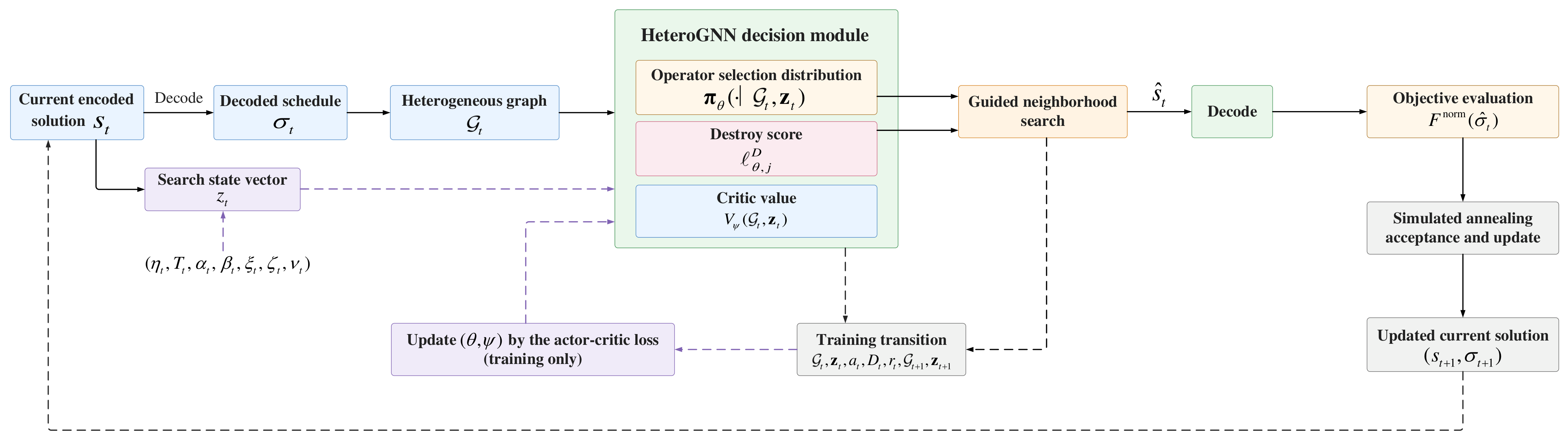
The framework of HeteroGNN-ALNS is illustrated in Figure 3.

The objective difference used in the acceptance decision is calculated from the normalized scalar objective as

$$\Delta F_t=F^{\mathrm{norm}}\left({\widehat{\sigma }}_t\right)-F^{\mathrm{norm}}\left({\sigma }_t\right).$$

(43)

The candidate schedule is accepted according to the SA acceptance criterion. The corresponding acceptance probability is given by

$$P_{\mathrm{acc}}({\widehat{\sigma }}_t\mid {\sigma }_t)=\left\{\begin{array}{cc}1,\hfill & \Delta F_t\le 0,\hfill \\ \exp (-\Delta F_t/T_t),\hfill & \Delta F_t>0.\hfill \end{array}\right.$$

(44)

The temperature schedule is given by

$$T_t=T_0{\left({\displaystyle \frac{T_{\min }}{T_0}}\right)}^{t/I_{\max }},$$

(45)

where $T_0$ and $T_{\min }$ denote the initial and final temperatures, respectively.

The adaptive operator weights of ALNS are used to select the operator when the HeteroGNN is not invoked. Let $w_{a,t}$ denote the weight of operator $a\in \mathsf{\Omega }$. The selection probability of operator a is given by

$$P_t\left(a\right)={\displaystyle \frac{w_{a,t}}{{\sum }_{a^{\prime }\in \mathsf{\Omega }}{w}_{a^{\prime },t}}}.$$

(46)

The operator weights are updated periodically according to

$$w_{a,t+1}=(1-\rho )w_{a,t}+\rho {\overline{\delta }}_{a,t},$$

(47)

where $\rho$ denotes the reaction factor and ${\overline{\delta }}_{a,t}$ denotes the average score of operator a in the current update segment.

To evaluate the contribution of each guided search transition to the search process, a reward is assigned according to

$$r_t=\kappa \left[F^{\mathrm{norm}}\left({\sigma }_t\right)-F^{\mathrm{norm}}\left({\widehat{\sigma }}_t\right)\right]+b_t,$$

(48)

where $\kappa$ denotes the reward scaling coefficient. The normalized objective difference measures the improvement of the candidate schedule, and the bonus $b_t$ reflects the search outcome relative to the best schedule.

The model parameters are updated using an actor–critic loss that incorporates the auxiliary destroy objective ${\mathsf{\Lambda }}_t^D$ defined in Equation (41). The loss consists of the policy objective for operator selection, the auxiliary destroy objective, the value function loss, and an entropy term. It is given by

$$\begin{array}{cc}\hfill \mathcal{L}(\theta ,\psi )=& -{\displaystyle \frac{1}{\left|\mathcal{B}\right|}}\sum _{t\in \mathcal{B}}\log {\pi }_{\theta }\left(a_t\mid {\mathcal{G}}_t,{\mathbf{z}}_t\right){\widehat{A}}_t\hfill \\ & -{\displaystyle \frac{1}{\left|\mathcal{B}\right|}}\sum _{t\in \mathcal{B}}{\mathsf{\Lambda }}_t^D{\widehat{A}}_t\hfill \\ & +{\displaystyle \frac{c_V}{\left|\mathcal{B}\right|}}\sum _{t\in \mathcal{B}}\mathrm{SmoothL1}\left(V_{\psi }({\mathcal{G}}_t,{\mathbf{z}}_t)-{\widehat{R}}_t\right)-{\displaystyle \frac{c_H}{\left|\mathcal{B}\right|}}\sum _{t\in \mathcal{B}}{H}_t,\hfill \end{array}$$

(49)

where $\mathcal{B}$ contains the transitions collected at iterations in which the HeteroGNN is invoked. The policy objective and the auxiliary destroy objective are weighted by the estimated advantage ${\widehat{A}}_t$, while the estimated return ${\widehat{R}}_t$ is used as the target of the critic. The coefficients $c_V$ and $c_H$ control the contributions of the value function loss and the entropy term, respectively, and $H_t$ denotes the entropy of the operator policy.

Only the transitions in $\mathcal{B}$ are used for model training. Consecutive transitions in $\mathcal{B}$ are treated as consecutive learning steps when generalized advantage estimation (GAE) is applied. One execution of the search procedure constitutes one training episode, and the model parameters are updated at the end of each episode.

Remark 2.

To reduce the dependence of the policy decision on information outside the current state representation, the heterogeneous graph encodes the current schedule, while the search-state vector incorporates recent ALNS search statistics. The state representation and adaptive control adopted in HeteroGNN-ALNS follow related DRL-guided metaheuristic frameworks in which information from the current search process is incorporated into learning-based search decisions [26,40]. The actor–critic training follows the general policy-gradient framework established in previous theoretical studies [41,42]. A formal convergence analysis for the coupled HeteroGNN-ALNS process requires further verification of the Markov property and the associated convergence conditions and is left for future study.

The overall procedure is summarized in Algorithm 2.

Algorithm 2 HeteroGNN-guided ALNS

Require: Instance data, maximum number of iterations $I_{\max }$, HeteroGNN invocation interval $K_G$ Ensure: Best schedule ${\sigma }^{*}$   1: Construct the initial encoded solution $s_0$ and obtain ${\sigma }_0\leftarrow \mathrm{Decode}(s_0,1)$   2: Set ${\sigma }_0^{*}\leftarrow {\sigma }_0$ and initialize $w_{a,0}$ for $a\in \mathsf{\Omega }$   3: for $t=0,1,\dots ,I_{\max }-1$ do   4:     Compute $T_t$ by Equation (45)   5:     if $t\mathrm{mod}{K}_G=0$ then   6:         Construct ${\mathcal{G}}_t$ from ${\sigma }_t$ and obtain ${\mathbf{z}}_t$   7:         Select $a_t$ by Equation (35) for training or Equation (36) for inference   8:         Construct $D_t$ according to Equations (37)–(40)   9:         Generate ${\widehat{s}}_t$ by Equation (42) 10:     else 11:         Select $a_t$ according to $P_t\left(a\right)$ in Equation (46) 12:         Generate ${\widehat{s}}_t$ from $s_t$ using the selected operator 13:     end if 14:     Obtain ${\widehat{\sigma }}_t\leftarrow \mathrm{Decode}({\widehat{s}}_t,K_R)$ 15:     Compute $\Delta F_t$ by Equation (43) 16:     Accept or reject $({\widehat{s}}_t,{\widehat{\sigma }}_t)$ by Equation (44) and obtain $(s_{t+1},{\sigma }_{t+1})$ 17:     Set ${\sigma }_{t+1}^{*}\leftarrow \arg {\min }_{\sigma \in \{{\sigma }_t^{*},{\sigma }_{t+1}\}}{F}^{\mathrm{norm}}\left(\sigma \right)$ 18:     if the current ALNS update segment is completed then 19:         Update $w_{a,t}$ by Equation (47) 20:     end if 21:     if $t\mathrm{mod}{K}_G=0$ and model training is performed then 22:         Compute $r_t$ by Equation (48) and ${\mathsf{\Lambda }}_t^D$ by Equation (41) 23:         Store the guided search transition 24:     end if 25: end for 26: if model training is performed then 27:     Update $(\theta ,\psi )$ by Equation (49) 28: end if 29: return ${\sigma }_{I_{\max }}^{*}$

5. Computational Experiments

5.1. Experimental Setup

The experiments are based on historical production records from a panel furniture factory. The records are collected over a continuous production period from multiple workshops. Customer orders are decomposed into panel jobs that pass through cutting, edge banding, drilling, and sorting. The corresponding numbers of production resources are 6, 1, 8, and 3, respectively. The number of panel jobs varies across production batches, and the selected job scales cover the range observed in the collected records. The instances are generated by randomly sampling N panel jobs from the production records, where $N\in \{50,100,150,200,300\}$. For each instance, the perturbation amplitudes of the processing and transport times are randomly sampled from 0 to 25% and 0 to 15%, respectively.

Four representative production conditions encountered in actual production are considered in the experiments. Normal production (Normal) retains the original production structure. Machine breakdown (MB) randomly sets one to three drilling machines as unavailable, which represents temporary machine unavailability caused by maintenance or faults. Job cancellation (JC) randomly removes 5% to 25% of the jobs at the edge banding and drilling stages to characterize the removal of panels identified as unsuitable during manual inspection. Topology change (TC) randomly disables one to four feasible transport connections between drilling and sorting to represent temporary changes caused by conveyor maintenance or material routing adjustments. The transport times of one to three connections between edge banding and drilling are multiplied by a random factor ranging from 0.5 to 2.0 to represent adjustments of roller conveyor speed.

The instances used for training and evaluation are generated independently with different random seeds. The training set contains 16 instances, with four instances generated for each production condition and N selected from the values given above. Each training episode uses one instance randomly selected from the training set. The evaluation instances are generated separately from the training instances. Unless otherwise stated, each search method is run five times with different random seeds on each evaluation instance, whereas Polling, shortest processing time (SPT), and longest processing time (LPT) are evaluated once.

HeteroGNN-ALNS is compared with Polling, SPT, LPT, Default ALNS [10], iterated greedy (IG) [43], and deep reinforced adaptive large neighborhood search (DR-ALNS) [26]. Polling, SPT, and LPT are used as dispatching rules, while Default ALNS, IG, and DR-ALNS are used as search baselines. Gurobi [44] and OR-Tools CP-SAT [45] are additionally used as exact solvers for the small-instance comparison. All methods are evaluated on the same instances under the same production conditions.

The weighted normalized score defined in Equations (18)–(20) is used as the main performance measure. The reference set ${\mathcal{S}}^{\mathrm{ref}}$ consists of the schedules decoded from the original job sequence, $R=5$ random sequences, the SPT sequence, and the LPT sequence. The objective weights are set to ${\omega }_C=0.7$, ${\omega }_W=0.2$, and ${\omega }_L=0.1$. Average completion time, average waiting time, normalized workload imbalance, and makespan are also reported.

The reward parameters are set according to preliminary experiments. The reward scaling coefficient $\kappa =10$ scales the typical normalized objective difference of approximately ${10}^{-2}$ to a magnitude comparable with $b_t$. A larger bonus is assigned to improvement of the best schedule to strengthen exploitation, while a positive bonus is retained for an accepted candidate without such improvement to encourage exploration. The bonus is specified as

$$b_t=\left\{\begin{array}{cc}5,\hfill & \mathrm{if} \mathrm{the} \mathrm{best} \mathrm{schedule} \mathrm{is} \mathrm{improved},\hfill \\ 1,\hfill & \mathrm{if} \mathrm{the} \mathrm{candidate} \mathrm{schedule} \mathrm{is} \mathrm{accepted} \mathrm{without} \mathrm{such} \mathrm{improvement},\hfill \\ -0.5,\hfill & \mathrm{otherwise}.\hfill \end{array}\right.$$

All experiments were conducted on a computing server with one 32 GB vGPU, 16 vCPUs, and 62 GB of memory using Python 3.12.7, PyTorch 2.2.2, and PyTorch Geometric 2.7.0. The main parameters of ALNS were selected with reference to previous studies [10,11,26] and adjusted according to preliminary experiments for the considered production setting. The HeteroGNN invocation interval $K_G$ was further examined through the sensitivity analysis in Section 5.5. The algorithm and learning settings are summarized in

Table 3. Algorithm and training settings.

Parameter	Setting
Algorithm settings
$n_{\min }^D$	10
${\lambda }_D$	0.08
$T_0,T_{\min }$	0.05, 0.001
$\rho$	0.2
ALNS weight update interval	15 iterations
$K_R$	3
$K_G$	3 iterations
$p_G$	0.7
$T_D$	1.0
${\lambda }_G$	0.5
Training settings
L	3
Hidden dimension	64
Dropout	0.1
Search statistics window	50 iterations
$\kappa$	10
$b_t$	5, 1, $-0.5$
Training episodes	600
Iterations per episode	200
Optimizer	Adam
Learning rate	$3\times {10}^{-4}$
$\gamma$	0.99
${\lambda }_{\mathrm{GAE}}$	0.95
$c_V$	0.1
$c_H$	0.02

.

5.2. Main Results

5.2.1. Training Process

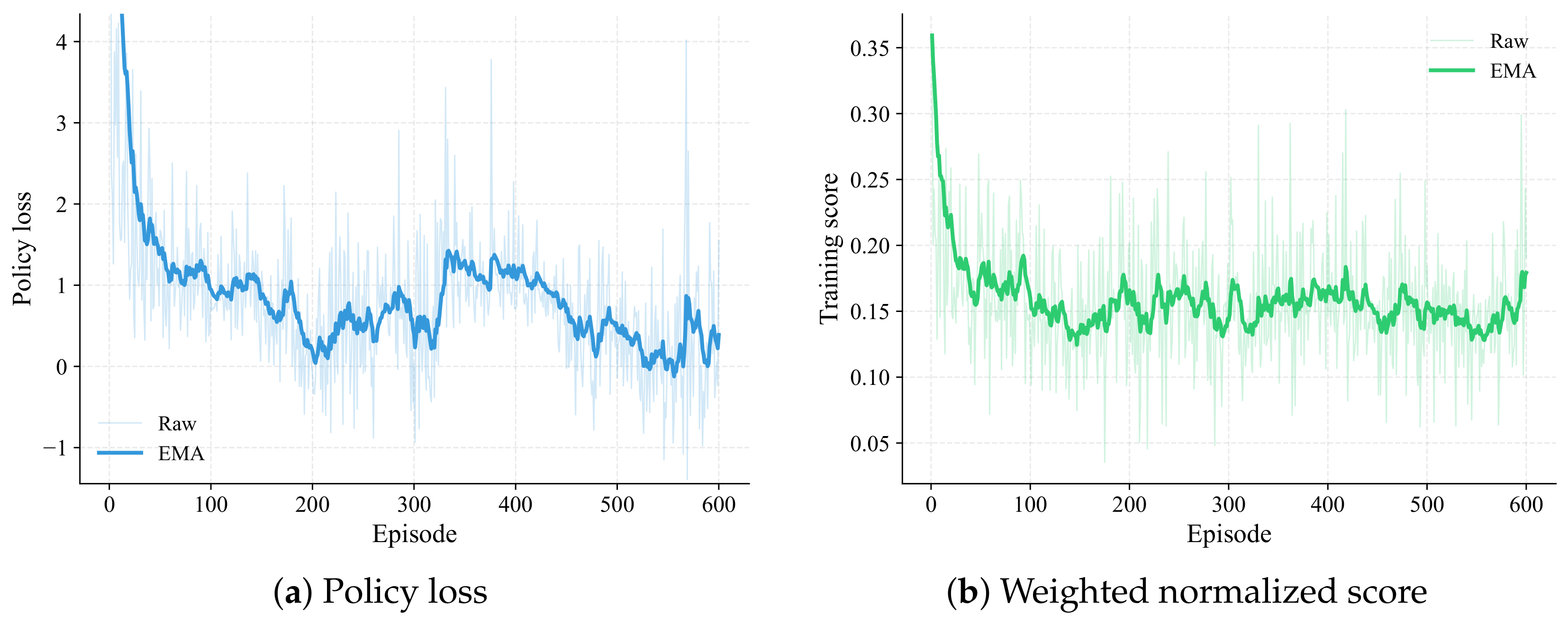
Figure 4 presents the training curves of HeteroGNN-ALNS. The policy loss decreases during the early episodes and subsequently fluctuates within a relatively stable range. The training score shows a clearer downward trend and gradually stabilizes as training proceeds. The variation between episodes is mainly associated with the different training instances and the stochastic decisions in the search, while the exponential moving average shows the overall trend more clearly.

5.2.2. Computational Efficiency

To examine the computational cost introduced by HeteroGNN inference and its effect on search performance, the search methods are compared under the equal-time setting and the equal-evaluation setting in

Table 4. Comparison under equal-time and equal-evaluation settings.

Setting	Method	${\mathit{F}}^{\mathbf{norm}}$	${\mathit{C}}_{\mathbf{avg}}$	${\mathit{W}}_{\mathbf{avg}}$	${\tilde{\mathit{f}}}_{\mathit{L}}$	Makespan	Runtime (s)	Evaluations
Equal time	Default ALNS	0.3743	80,399.2	1344.5	0.3933	139,642.0	5.013	213.1
	IG	0.3240	75,873.4	1161.6	0.5573	141,618.5	5.011	213.7
	DR-ALNS	0.4112	80,935.2	1499.1	0.5902	142,401.8	5.013	200.3
	HeteroGNN-ALNS	0.1593	61,921.8	1098.5	0.4979	140,955.5	5.018	155.3
Equal evaluation	Default ALNS	0.3653	79,801.9	1296.2	0.3968	139,587.3	6.824	270.0
	IG	0.3242	76,683.1	1056.1	0.4947	140,840.3	6.798	270.0
	DR-ALNS	0.3912	80,040.3	1446.7	0.5315	141,196.1	7.229	270.0
	HeteroGNN-ALNS	0.1131	58,228.3	1105.6	0.4139	139,837.3	9.046	270.0

. HeteroGNN-ALNS obtains the lowest weighted normalized score under both settings. Under the equal-time setting, HeteroGNN-ALNS performs fewer evaluations than Default ALNS but still obtains a lower weighted normalized score. This result shows that the improvement is associated with more effective search guidance rather than more candidate evaluations.

Under the equal-time setting, HeteroGNN-ALNS obtains a weighted normalized score 57.4% lower than that of Default ALNS while evaluating 27.1% fewer candidate schedules. The smaller number of evaluations reflects the additional computation required for graph construction and HeteroGNN inference, while the average completion time and average waiting time are reduced by 23.0% and 18.3%, respectively. Default ALNS gives lower normalized workload imbalance and makespan, which have smaller weights in the scalar objective.

Under the equal-evaluation setting, HeteroGNN-ALNS again gives the lowest weighted normalized score and average completion time, with reductions of 69.0% and 27.0% relative to Default ALNS. IG gives a 4.5% lower average waiting time than HeteroGNN-ALNS, while its average completion time is 31.7% higher. The runtime of HeteroGNN-ALNS increases to 9.046 s because each guided iteration additionally requires graph construction and HeteroGNN inference.

5.2.3. Computational Cost

To further examine the computational cost of HeteroGNN-ALNS, the runtime of graph construction, search-state vector construction, HeteroGNN inference, destroy selection, repair, schedule decoding, and objective evaluation is measured at different job scales. With fixed network settings, the computational complexity of graph construction and message passing can be expressed as $O\left(\right|{\mathcal{V}}_t|+|{\mathcal{E}}_t\left|\right)=O\left(N\right)$. According to Equation (23) and the numbers of production resources, the heterogeneous graph contains $N+18$ nodes. The edge set contains $8N$ assignment edges, $2(N-1)$ sequence edges, and at most 68 transport edges after reverse relations are included. Thus, $\left|{\mathcal{E}}_t\right|\le 8N+2(N-1)+68=10N+66$. Both $|{\mathcal{V}}_t|$ and $|{\mathcal{E}}_t|$ scale linearly with N. Schedule decoding also has a complexity of $O\left(N\right)$ because the numbers of candidate resources at each production stage are fixed. Accordingly, graph construction and message passing have $O\left(N\right)$ complexity per HeteroGNN invocation, and schedule decoding has $O\left(N\right)$ complexity per evaluation. For application to another manufacturing process, the numbers of resource nodes and feasible edges are adjusted according to the production topology, while the HeteroGNN architecture and training procedure remain unchanged.

As shown in

Table 5. Runtime of the main computational components.

Component	N
	50	100	200	300
HeteroGNN invocation (ms/call)
Graph construction	1.70	1.60	1.80	2.00
Search-state vector construction	0.08	0.06	0.05	0.05
HeteroGNN inference	17.30	17.80	17.30	16.30
Destroy selection	0.88	0.83	1.00	1.37
Solution evaluation (ms/evaluation)
Repair	0.02	0.03	0.03	0.04
Schedule decoding	4.52	9.06	18.24	26.93
Objective evaluation	0.03	0.04	0.06	0.08

, schedule decoding time increases approximately with the job scale, which is consistent with the sequential decoding procedure in Algorithm 1. In contrast, graph construction and HeteroGNN inference show only small variations over the tested job scales, although $|{\mathcal{V}}_t|$ and $|{\mathcal{E}}_t|$ increase linearly with N. The limited increase in graph construction time may be attributed to the relatively large proportion of fixed computational overhead within the evaluated range. The small variation in inference time may result from parallel computation in HeteroGNN inference. Since the HeteroGNN is invoked every $K_G=3$ iterations, the additional computation associated with graph processing and inference is distributed over multiple search iterations.

5.2.4. Performance with Different Numbers of Jobs

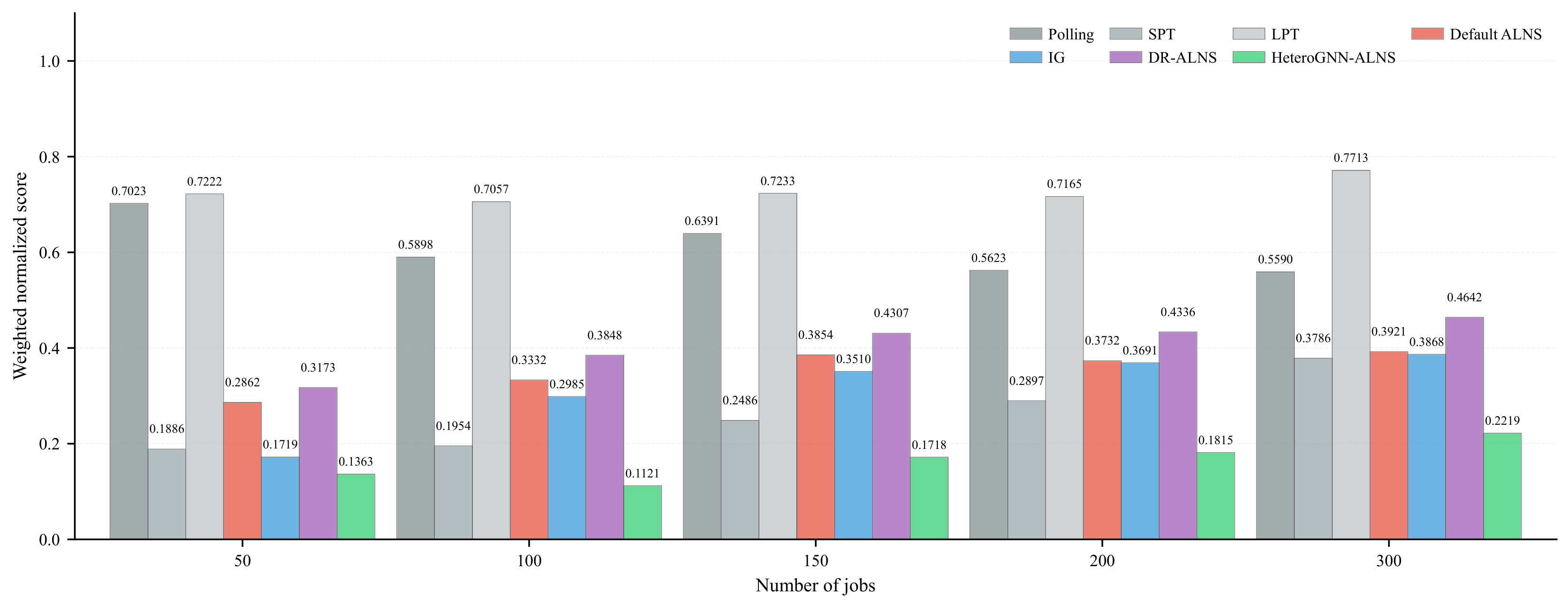
Figure 5 compares the weighted normalized scores obtained with different numbers of jobs. HeteroGNN-ALNS gives the lowest score for all values of N, with reductions of 43.4% to 66.4% relative to Default ALNS. Its average completion time is also reduced by 13.3% to 22.9%.

The individual performance indicators are reported in

Table 6. Performance for different numbers of jobs.

N	Method	${\mathit{F}}^{\mathbf{norm}}$	${\mathit{C}}_{\mathbf{avg}}$	${\mathit{W}}_{\mathbf{avg}}$	${\tilde{\mathit{f}}}_{\mathit{L}}$	Makespan
50	Polling	0.7023	54,430.8	2011.0	0.7820	79,437.8
	SPT	0.1886	36,904.1	949.3	0.9065	81,063.4
	LPT	0.7222	60,400.3	1177.8	0.0362	67,803.9
	Default ALNS	0.2862	43,785.0	487.9	0.4824	74,066.6
	IG	0.1719	39,153.6	375.2	0.6045	76,042.8
	DR-ALNS	0.3173	44,581.9	672.3	0.4442	73,581.4
	HeteroGNN-ALNS	0.1363	37,948.0	500.3	0.4579	73,885.8
100	Polling	0.5898	69,707.9	2013.0	0.6125	109,069.8
	SPT	0.1954	45,006.2	1447.7	0.9795	115,650.3
	LPT	0.7057	85,433.6	714.7	0.1949	102,966.5
	Default ALNS	0.3332	61,556.7	965.6	0.2455	103,802.2
	IG	0.2985	58,986.2	849.5	0.3634	105,547.5
	DR-ALNS	0.3848	63,492.3	1160.6	0.2924	104,567.5
	HeteroGNN-ALNS	0.1121	48,602.8	897.3	0.1942	103,024.6
150	Polling	0.6391	92,920.4	2447.7	0.7968	155,358.6
	SPT	0.2486	55,327.2	2255.1	0.8965	156,685.5
	LPT	0.7233	118,859.0	636.0	0.4526	148,704.9
	Default ALNS	0.3854	84,027.9	1414.5	0.2438	145,572.9
	IG	0.3510	82,415.0	1135.9	0.2988	146,430.3
	DR-ALNS	0.4307	85,857.8	1528.8	0.3652	147,492.5
	HeteroGNN-ALNS	0.1718	64,805.9	1080.0	0.3591	147,427.1
200	Polling	0.5623	109,645.1	2555.4	0.6564	189,450.9
	SPT	0.2897	64,967.9	3180.4	0.9175	194,212.1
	LPT	0.7165	147,010.8	616.9	0.4778	186,303.5
	Default ALNS	0.3732	101,031.6	1620.7	0.2147	181,437.9
	IG	0.3691	101,113.3	1423.2	0.2931	182,673.4
	DR-ALNS	0.4336	104,693.3	1889.8	0.3297	183,191.0
	HeteroGNN-ALNS	0.1815	78,993.0	1324.1	0.2972	182,745.5
300	Polling	0.5590	151,600.2	2485.8	0.7145	270,662.1
	SPT	0.3786	87,638.8	5144.1	0.8161	270,662.3
	LPT	0.7713	207,811.1	659.3	0.8149	270,644.6
	Default ALNS	0.3921	139,065.7	2014.0	0.2034	259,161.3
	IG	0.3868	140,767.1	1736.9	0.2057	259,123.8
	DR-ALNS	0.4642	146,689.4	2254.9	0.3060	260,808.7
	HeteroGNN-ALNS	0.2219	110,961.9	1749.6	0.2099	259,119.3

. For $N=100$ to 300, HeteroGNN-ALNS reduces the average waiting time of Default ALNS by 7.1% to 23.6%. At $N=50$, Default ALNS gives a 2.5% lower average waiting time because changes in the positions of a small number of jobs have a greater influence on the average waiting time when fewer sequencing decisions are involved.

SPT gives the lowest average completion time for all values of N because jobs with shorter processing times are given priority. Its average waiting time is 61.3% to 194.0% higher than that of HeteroGNN-ALNS because the rule does not consider waiting at subsequent production stages.

LPT gives priority to jobs with longer processing times and produces lower average waiting times than HeteroGNN-ALNS for $N=100$ to 300. Its average completion time is 75.8% to 87.3% higher because scheduling longer jobs first delays a larger number of shorter jobs.

IG obtains slightly lower average waiting times at several values of N, while its average completion time and weighted normalized score remain higher than those of HeteroGNN-ALNS. Compared with DR-ALNS, HeteroGNN-ALNS reduces the weighted normalized score by 52.2% to 70.9% and the average waiting time by 22.4% to 29.9%. The main difference is that HeteroGNN-ALNS uses the heterogeneous graph and search state vector to guide both operator selection and destroy set construction. The differences in normalized workload imbalance among the search methods are comparatively small.

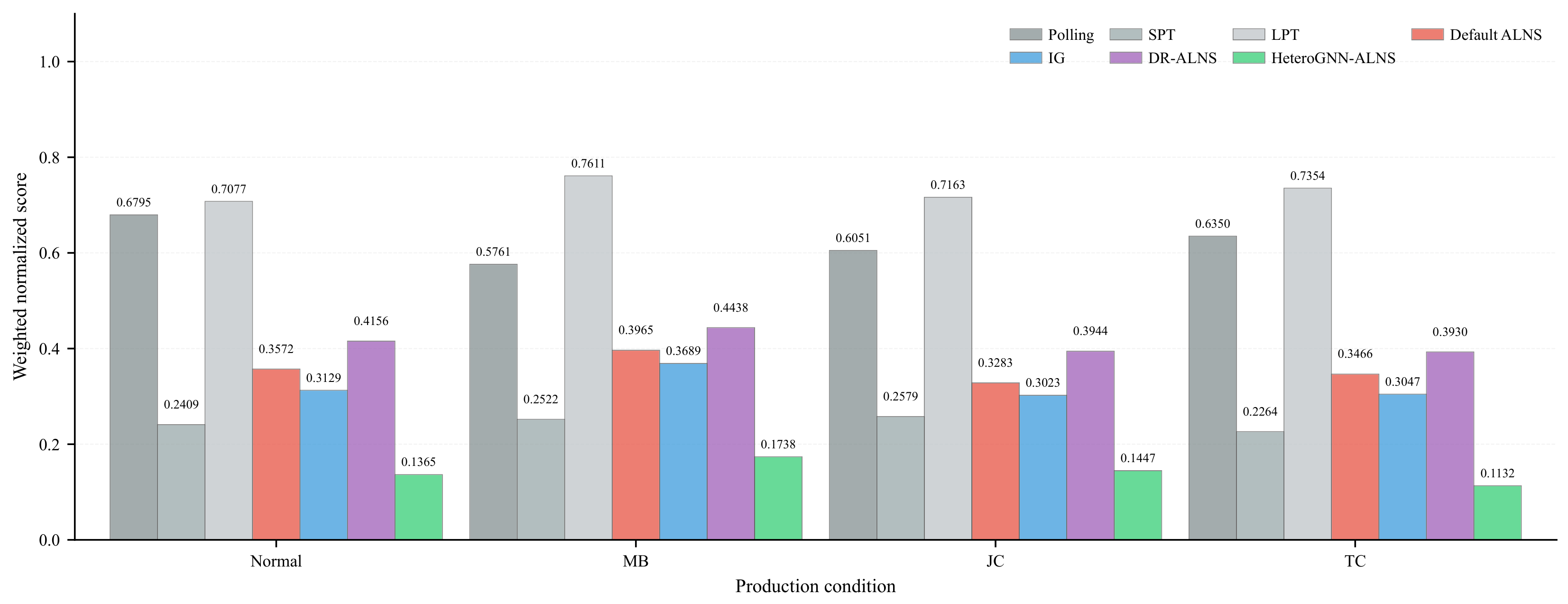
5.2.5. Performance Under Different Production Conditions

The performance under different production conditions is further compared in Figure 6. HeteroGNN-ALNS gives the lowest weighted normalized score under all four conditions. Compared with Default ALNS, the score is reduced by 55.9% to 67.3%, accompanied by reductions of 20.1% to 22.7% in average completion time and 11.1% to 19.1% in average waiting time.

The individual performance indicators under the four production conditions are reported in

Table 7. Performance under different production conditions.

Condition	Method	${\mathit{F}}^{\mathbf{norm}}$	${\mathit{C}}_{\mathbf{avg}}$	${\mathit{W}}_{\mathbf{avg}}$	${\tilde{\mathit{f}}}_{\mathit{L}}$	Makespan
Normal	Polling	0.6795	80,713.7	2395.3	0.8910	130,567.0
	SPT	0.2409	49,257.9	2098.7	0.9397	131,142.2
	LPT	0.7077	98,333.7	673.7	0.2567	120,771.0
	Default ALNS	0.3572	70,173.2	1075.9	0.2746	120,778.6
	IG	0.3129	67,213.0	894.5	0.4061	122,644.2
	DR-ALNS	0.4156	73,056.3	1222.4	0.3434	121,833.5
	HeteroGNN-ALNS	0.1365	54,739.9	905.3	0.2915	121,036.1
MB	Polling	0.5761	86,151.7	1911.9	0.6126	140,812.6
	SPT	0.2522	53,244.1	2099.6	0.9725	148,809.2
	LPT	0.7611	111,099.5	689.6	0.3558	137,329.2
	Default ALNS	0.3965	77,619.4	1409.9	0.2907	134,366.2
	IG	0.3689	76,177.7	1121.9	0.3721	135,915.9
	DR-ALNS	0.4438	80,180.9	1620.0	0.3051	135,041.2
	HeteroGNN-ALNS	0.1738	60,436.6	1149.1	0.2733	134,118.9
JC	Polling	0.6051	80,277.4	2097.8	0.6735	129,247.3
	SPT	0.2579	49,755.2	2089.0	0.9879	134,080.5
	LPT	0.7163	101,021.9	745.4	0.3330	123,622.2
	Default ALNS	0.3283	71,027.0	1040.4	0.2911	123,271.1
	IG	0.3023	69,376.6	928.2	0.3928	124,864.5
	DR-ALNS	0.3944	73,867.6	1279.6	0.3765	124,530.2
	HeteroGNN-ALNS	0.1447	56,777.9	924.8	0.3245	123,739.7
TC	Polling	0.6350	77,194.1	2188.9	0.7740	123,960.4
	SPT	0.2264	47,973.4	1992.3	0.9322	126,179.6
	LPT	0.7354	95,699.4	761.6	0.4091	117,945.4
	Default ALNS	0.3466	68,355.1	1122.1	0.2763	115,752.9
	IG	0.3047	66,210.4	921.2	0.3745	117,158.7
	DR-ALNS	0.3930	69,911.5	1299.2	0.3439	116,810.9
	HeteroGNN-ALNS	0.1132	52,860.6	907.9	0.3006	116,085.9

. HeteroGNN-ALNS achieves the lowest weighted normalized score among the compared methods under all four production conditions. LPT gives lower average waiting times, whereas its average completion time is 77.9% to 83.8% higher than that of HeteroGNN-ALNS because longer jobs are given priority. SPT shows the opposite tendency, with lower average completion times but considerably higher average waiting times.

The differences between HeteroGNN-ALNS and the other search methods remain consistent across the four production conditions. Compared with DR-ALNS, the weighted normalized score is reduced by 60.8% to 71.2%. IG gives similar or slightly lower average waiting times in several conditions, while HeteroGNN-ALNS gives substantially lower average completion times and better overall performance.

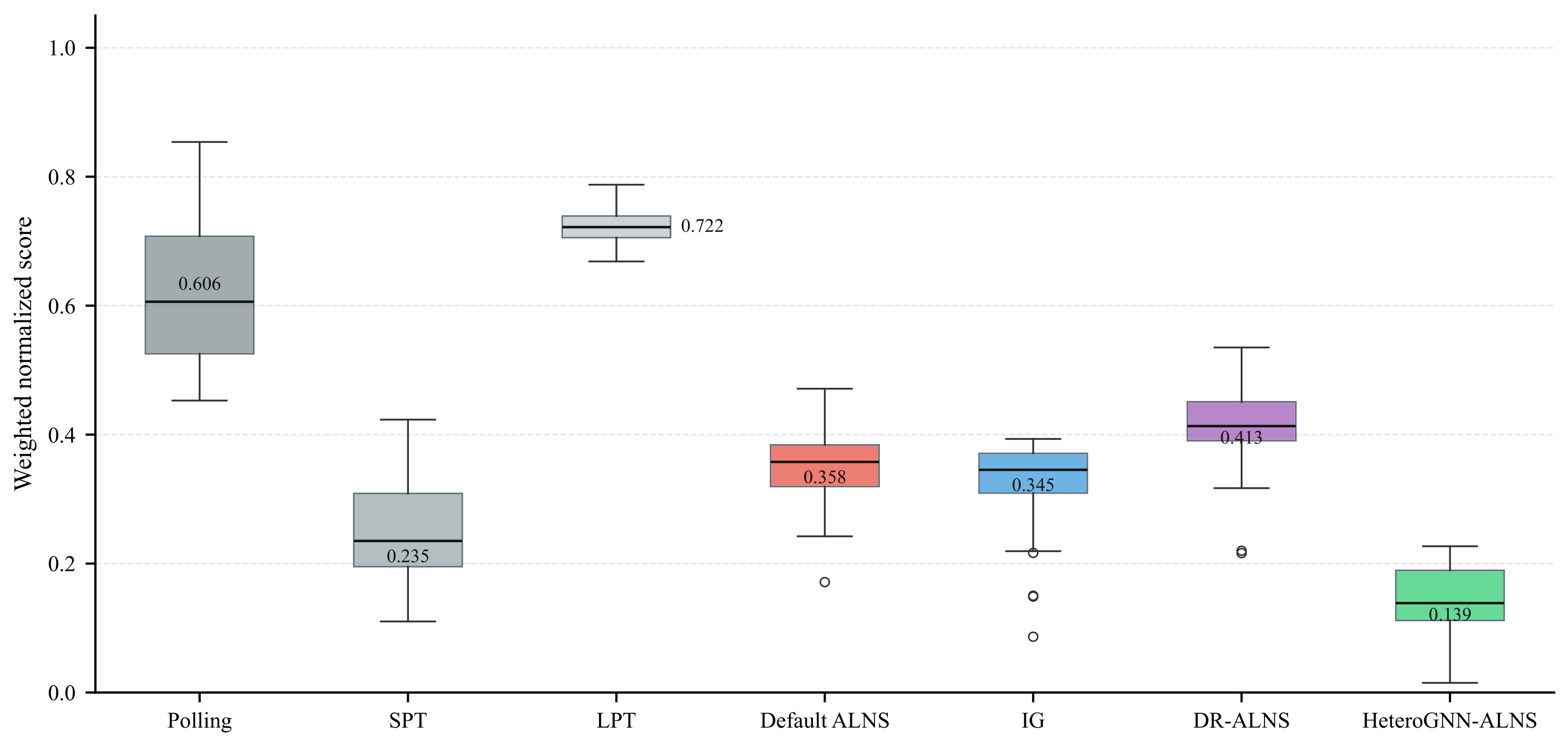
Figure 7 further presents the distribution of weighted normalized scores across the production conditions. HeteroGNN-ALNS has the lowest median and a relatively narrow interquartile range, which indicate better overall performance and greater consistency across the tested production conditions.

5.3. Statistical Analysis

The weighted normalized score is used for the statistical analysis because it combines the three scheduling criteria in the objective function. For each production condition and method, the results from repeated runs are first averaged for each instance. The resulting values form paired samples for comparisons between HeteroGNN-ALNS and Default ALNS, IG, and DR-ALNS.

A Wilcoxon signed-rank test is applied to each paired comparison using the one-sided alternative hypothesis that HeteroGNN-ALNS obtains a lower weighted normalized score than the corresponding baseline. The Holm procedure is used to adjust the p-values from the twelve comparisons and control the familywise error rate. The effect size is measured by the rank-biserial correlation.

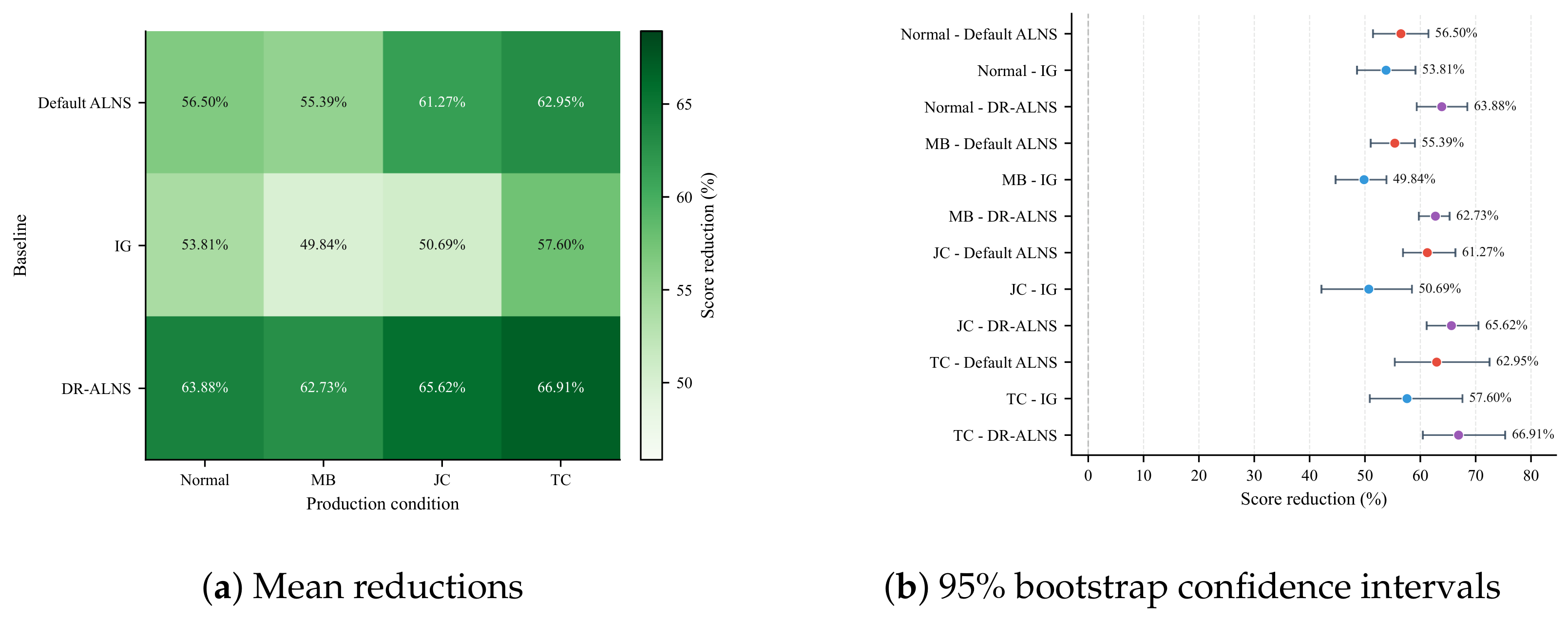
All twelve comparisons give $p=0.000977$ before correction and $p=0.011719$ after the Holm correction. The differences therefore remain statistically significant at the 5% level. The rank-biserial correlation is $1.0$ in every comparison, indicating that the weighted normalized score of HeteroGNN-ALNS is lower for every paired instance. Figure 8 presents the mean score reductions together with their 95% bootstrap confidence intervals.

5.4. Ablation Study

The contribution of the main components of HeteroGNN-ALNS is examined through the ablation study reported in

Table 8. Ablation study results.

Setting	${\mathit{F}}^{\mathbf{norm}}$	${\mathit{C}}_{\mathbf{avg}}$	${\mathit{W}}_{\mathbf{avg}}$	${\tilde{\mathit{f}}}_{\mathit{L}}$	Makespan
Full model	0.1332	59,021.7	975.5	0.4155	135,362.2
Without search state vector	0.1451	60,033.8	943.5	0.4873	136,020.6
Without relation-specific message passing	0.1394	59,930.2	993.5	0.3086	134,385.3
Homogeneous graph	0.1618	61,683.3	943.3	0.4118	135,219.1
Without operator head	0.1868	63,257.6	989.5	0.4215	135,329.5
Without destroy head	0.1638	62,029.5	1067.3	0.2842	134,117.3

. The full model is compared with variants in which the search state vector, relation-specific message passing, heterogeneous graph representation, operator head, or destroy head is removed.

The weighted normalized score increases when either the search state vector or relation-specific message passing is removed, which supports the necessity of both components in HeteroGNN-ALNS. A larger increase is observed when the heterogeneous graph is replaced by a homogeneous graph, while the average completion time also increases. The distinction between different node types and relations therefore provides useful information for representing the current scheduling state.

Among the ablated components, removal of the two decision heads produces the largest increases in the weighted normalized score, which shows that operator selection and destroy set construction have the largest effects on the overall objective. The weighted normalized score increases most after removal of the operator head, and removal of the destroy head further increases the average waiting time. Although the latter variant gives lower normalized workload imbalance and makespan, its average completion time and average waiting time are higher under the objective weights used in this study.

5.5. Sensitivity Analysis

The sensitivity of the proposed method to the HeteroGNN invocation interval $K_G$ is examined in

Table 9. Sensitivity analysis of $K_G$.

${\mathit{K}}_{\mathit{G}}$	${\mathit{F}}^{\mathbf{norm}}$	${\mathit{C}}_{\mathbf{avg}}$	${\mathit{W}}_{\mathbf{avg}}$	${\tilde{\mathit{f}}}_{\mathit{L}}$	Makespan
1	0.1518	56,675.5	1239.9	0.6887	139,801.0
3	0.1507	60,588.5	979.3	0.4617	137,156.4
5	0.1834	63,397.1	998.1	0.4323	136,708.6
10	0.2135	66,340.0	959.8	0.3894	136,383.6

.

The lowest weighted normalized score is obtained with $K_G=3$. The weighted normalized score is higher at $K_G=5$ and $K_G=10$, mainly because less frequent HeteroGNN invocation leads to a larger average completion time. The setting $K_G=1$ gives a slightly higher weighted normalized score than $K_G=3$ despite its lower average completion time because its average waiting time, normalized workload imbalance, and makespan are higher. Therefore, $K_G=3$ is adopted in the main experiments.

The sensitivity to the number R of random sequences in ${\mathcal{S}}^{\mathrm{ref}}$ is further examined with $R\in \{0,5,10,20,50,100\}$. The normalization bounds are reconstructed with each value of R. The same evaluated schedules are rescored under the corresponding bounds. The setting $R=5$ is adopted in the main experiments. The mean absolute difference in $F^{\mathrm{norm}}$ relative to $R=5$ is denoted by $\mathrm{Mean}|\Delta F^{\mathrm{norm}}|$.

Table 10. Sensitivity analysis of R.

R	Mean $|\mathbf{\Delta }{\mathit{F}}^{\mathbf{norm}}|$	Ranking Changes
0	0.0225–0.0641	1/30
5	0.0000	0/30
10	0.0127–0.0147	0/30
20	0.0144–0.0180	0/30
50	0.0192–0.0259	0/30
100	0.0220–0.0294	0/30

reports its range across the three evaluated methods. No ranking change is observed with $R\in \{10,20,50,100\}$. The corresponding $\mathrm{Mean}|\Delta F^{\mathrm{norm}}|$ remains below 0.03. One ranking change is observed at $R=0$ after exclusion of the random reference sequences. These results show that the inclusion of random reference sequences improves ranking stability, whereas increasing R beyond 5 has only a limited effect on $F^{\mathrm{norm}}$.

5.6. Comparison with Exact Solvers

Two independent exact formulations of the considered scheduling problem are implemented with Gurobi MIP and OR-Tools CP-SAT. Model correctness is examined on an instance with $N=6$. The optimal makespan and total completion time are compared with those obtained by exhaustive enumeration based on the scheduling decoder. In addition, the weighted objective $F^{\mathrm{norm}}$ is formulated as a linear objective in CP-SAT with the weights specified in Section 5.1 for the same instances. Five instances are considered for each of $N=10$ and $N=20$. The CP-SAT reference values $F^{*}$ range from 0.0012 to 0.0136 for $N=10$ and from $-0.057$ to 0.047 for $N=20$. The total completion time is compared with the best feasible solution obtained by CP-SAT within 600 s. The gap for the weighted objective is defined as $\Delta F=F^{\mathrm{norm}}-F^{*}$.

The results of Default ALNS and HeteroGNN-ALNS are reported as the mean and standard deviation over five instances and five random seeds. The results are summarized in

Table 11. Comparison with exact solvers on small instances.

(a) Model validation
Method		Makespan	Total Completion Time	${\mathit{F}}^{\mathbf{norm}}$
Gurobi MIP		42,986	162,575	–
OR-Tools CP-SAT		42,986	162,575	0.0254
Decoder enumeration		42,986	162,575	0.0702
(b) Gaps to solver references
$\mathit{N}$	Method	Makespan (%)	Total Completion Time (%)	ΔF
10	Default ALNS	$6.98\pm 2.79$	$7.93\pm 3.64$	$0.1711\pm 0.0504$
	HeteroGNN-ALNS	$7.15\pm 3.00$	$8.64\pm 2.86$	$0.1773\pm 0.0436$
20	Default ALNS	$13.99\pm 6.66$	$10.63\pm 4.91$	$0.2052\pm 0.0576$
	HeteroGNN-ALNS	$18.51\pm 6.28$	$5.49\pm 2.15$	$0.1568\pm 0.0325$

. Gurobi, CP-SAT, and exhaustive enumeration obtain identical optimal values for makespan and total completion time for $N=6$. All five $N=10$ instances and three of the five $N=20$ instances are proven optimal by the exact solvers for the makespan objective. The best-known solutions for the remaining two $N=20$ instances are within 1.32% and 0.16% of the corresponding lower bounds. HeteroGNN-ALNS gives higher gaps than Default ALNS for makespan. HeteroGNN-ALNS gives slightly higher gaps than Default ALNS for total completion time and $\Delta F$ at $N=10$, while lower gaps are obtained at $N=20$. This variation is consistent with the multi-objective formulation considered in this paper, as the search accounts for the combined effects of different scheduling objectives.

6. Conclusions

This study investigates the FJSP in panel furniture production under practical production requirements. A mathematical model is formulated to consider different processing times, variable transport resources, and specific production constraints. An ALNS method guided by a HeteroGNN, termed HeteroGNN-ALNS, is developed to solve the scheduling problem. The scheduling state in ALNS is represented as a heterogeneous graph and combined with a search state vector. Based on this representation, the HeteroGNN guides neighborhood operator selection and destroy set construction, and the guidance policy is trained using an actor–critic method.

Computational experiments are conducted under four production conditions and five job scales. Compared with Default ALNS, HeteroGNN-ALNS reduces the weighted normalized score by 43.4–66.4% across the five job scales and by 55.9–67.3% across the four production conditions. HeteroGNN-ALNS also achieves better overall scheduling performance under both equal-evaluation and equal-time settings. The statistical analysis based on the Wilcoxon signed-rank test with Holm correction confirms that HeteroGNN-ALNS significantly outperforms the main search baselines. The ablation study further verifies the contribution of each main component, with the operator head and destroy head having the largest effects on the weighted normalized score.

There are some limitations in this paper. The computational requirements for graph construction and HeteroGNN inference increase with the size of the scheduling graph. The current experiments are based on historical production records and offline scheduling instances. Future work will investigate the real-time performance of the proposed method for online rescheduling and evaluate the practical applicability of the proposed method when new jobs arrive.

References

1. Ouyang, Z.; Wu, Y.; Shao, H.; Wang, X.; Tao, T.; Chen, X.; Peng, T. Method for drill-bit arrangement in CNC woodworking drilling machine for mass customization. J. Manuf. Syst. 2025, 78, 200–212. [Google Scholar] [CrossRef] [Scilit]
2. Wang, J.; Wu, Z.; Yang, L.; Hu, W.; Song, C.; Zhu, Z.; Guo, X.; Cao, P. Investigation on distributed rescheduling with cutting tool maintenance based on NSGA-III in large-scale panel furniture intelligent manufacturing. J. Manuf. Process. 2024, 112, 214–224. [Google Scholar] [CrossRef] [Scilit]
3. Dauzère-Pèrès, S.; Ding, J.; Shen, L.; Tamssaouet, K. The flexible job shop scheduling problem: A review. Eur. J. Oper. Res. 2024, 314, 409–432. [Google Scholar] [CrossRef] [Scilit]
4. Chen, R.; Wu, B.; Wang, H.; Tong, H.; Yan, F. A Q-Learning based NSGA-II for dynamic flexible job shop scheduling with limited transportation resources. Swarm Evol. Comput. 2024, 90, 101658. [Google Scholar] [CrossRef] [Scilit]
5. Moon, S.; Lee, S.; Park, K.J. Learning-enabled flexible job-shop scheduling for scalable smart manufacturing. J. Manuf. Syst. 2024, 77, 356–367. [Google Scholar] [CrossRef] [Scilit]
6. Peng, N.; Zheng, Y.; Xiao, Z.; Gong, G.; Huang, D.; Liu, X.; Zhu, K.; Luo, Q. Multi-objective dynamic distributed flexible job shop scheduling problem considering uncertain processing time. Clust. Comput. 2025, 28, 185. [Google Scholar] [CrossRef] [Scilit]
7. Lei, K.; Guo, P.; Wang, Y.; Zhang, J.; Meng, X.; Qian, L. Large-scale dynamic scheduling for flexible job-shop with random arrivals of new jobs by hierarchical reinforcement learning. IEEE Trans. Ind. Inform. 2024, 20, 1007–1018. [Google Scholar] [CrossRef] [Scilit]
8. Li, J.; Li, X.; Gao, L.; Wang, C.; Chen, H. A multitasking workforce-constrained flexible job shop scheduling problem: An application from a real-world workshop. J. Manuf. Syst. 2025, 83, 196–215. [Google Scholar] [CrossRef] [Scilit]
9. Tamssaouet, K.; Dauzère-Pèrès, S. A general efficient neighborhood structure framework for the job-shop and flexible job-shop scheduling problems. Eur. J. Oper. Res. 2023, 311, 455–471. [Google Scholar] [CrossRef] [Scilit]
10. Ropke, S.; Pisinger, D. An adaptive large neighborhood search heuristic for the pickup and delivery problem with time windows. Transp. Sci. 2006, 40, 455–472. [Google Scholar] [CrossRef] [Scilit]
11. Liu, J.; Sun, B.; Li, G.; Chen, Y. Multi-objective adaptive large neighbourhood search algorithm for dynamic flexible job shop schedule problem with transportation resource. Eng. Appl. Artif. Intell. 2024, 132, 107917. [Google Scholar] [CrossRef] [Scilit]
12. Kasapidis, G.A.; Paraskevopoulos, D.C.; Mourtos, I.; Repoussis, P.P. A unified solution framework for flexible job shop scheduling problems with multiple resource constraints. Eur. J. Oper. Res. 2025, 320, 479–495. [Google Scholar] [CrossRef] [Scilit]
13. Johnn, S.N.; Darvariu, V.A.; Handl, J.; Kalcsics, J. Graph Reinforcement Learning for Operator Selection in the ALNS Metaheuristic. In Proceedings of the Optimization and Learning; Communications in Computer and Information Science; Springer: Cham, Switzerland, 2023; Volume 1824, pp. 200–212. [Google Scholar] [CrossRef] [Scilit]
14. Teichteil-Königsbuch, F.; Povéda, G.; González de Garibay Barba, G.; Luchterhand, T.; Thiébaux, S. Fast and Robust Resource-Constrained Scheduling with Graph Neural Networks. Proc. Int. Conf. Autom. Plan. Sched. 2023, 33, 623–633. [Google Scholar] [CrossRef] [Scilit]
15. Sui, J.; Ding, S.; Xia, B.; Liu, R.; Bu, D. NeuralGLS: Learning to guide local search with graph convolutional network for the traveling salesman problem. Neural Comput. Appl. 2024, 36, 9687–9706. [Google Scholar] [CrossRef] [Scilit]
16. Johnn, S.N.; Darvariu, V.A.; Handl, J.; Kalcsics, J. A graph reinforcement learning framework for neural adaptive large neighbourhood search. Comput. Oper. Res. 2024, 172, 106791. [Google Scholar] [CrossRef] [Scilit]
17. Duan, Y.; Li, M.; Shi, L.; Li, L.; Zhao, X.; He, L. A genetic-operator-integrated whale optimization algorithm for solving the flexible job shop scheduling problem. J. King Saud Univ.—Comput. Inf. Sci. 2025, 37, 259. [Google Scholar] [CrossRef] [Scilit]
18. Pisinger, D.; Ropke, S. Large Neighborhood Search. In Handbook of Metaheuristics; Gendreau, M., Potvin, J.Y., Eds.; Springer: Boston, MA, USA, 2010; pp. 399–419. [Google Scholar] [CrossRef] [Scilit]
19. Windras Mara, S.T.; Norcahyo, R.; Jodiawan, P.; Lusiantoro, L.; Rifai, A.P. A survey of adaptive large neighborhood search algorithms and applications. Comput. Oper. Res. 2022, 146, 105903. [Google Scholar] [CrossRef] [Scilit]
20. Anand Deva Durai, C.; Azath, M.; Jeniffer, J.S.C. Integrated search method for flexible job shop scheduling problem using HHS-ALNS algorithm. SN Comput. Sci. 2020, 1, 83. [Google Scholar] [CrossRef] [Scilit]
21. Liu, M.; Lv, J.; Du, S.; Deng, Y.; Shen, X.; Zhou, Y. Multi-resource constrained flexible job shop scheduling problem with fixture-pallet combinatorial optimisation. Comput. Ind. Eng. 2024, 188, 109903. [Google Scholar] [CrossRef] [Scilit]
22. Yunusoglu, P.; Topaloglu Yildiz, S. Solving the flexible job shop scheduling and lot streaming problem with setup and transport resource constraints. Int. J. Syst. Sci. Oper. Logist. 2023, 10, 2221072. [Google Scholar] [CrossRef] [Scilit]
23. Ji, B.; Zhang, S.; Yu, S.S.; Xiao, X.; Chen, C.; Zheng, G. Novel model and solution method for flexible job shop scheduling problem with batch processing machines. Comput. Oper. Res. 2024, 161, 106442. [Google Scholar] [CrossRef] [Scilit]
24. Wang, Y.; Xia, T.; Xu, Y.; Ding, Y.; Zheng, M.; Pan, E.; Xi, L. Joint optimization of flexible job shop scheduling and preventive maintenance under high-frequency production switching. Int. J. Prod. Econ. 2024, 269, 109163. [Google Scholar] [CrossRef] [Scilit]
25. Voigt, S. A review and ranking of operators in adaptive large neighborhood search for vehicle routing problems. Eur. J. Oper. Res. 2025, 322, 357–375. [Google Scholar] [CrossRef] [Scilit]
26. Reijnen, R.; Zhang, Y.; Lau, H.C.; Bukhsh, Z. Online control of adaptive large neighborhood search using deep reinforcement learning. Proc. Int. Conf. Autom. Plan. Sched. 2024, 34, 475–483. [Google Scholar] [CrossRef] [Scilit]
27. Wang, Z.; Cui, Q.; Tan, B.; Yang, X.; Zhou, W.; Huang, X. Reinforcement learning-guided adaptive large neighborhood search for vehicle routing problem with time windows. J. Comb. Optim. 2025, 50, 35. [Google Scholar] [CrossRef] [Scilit]
28. Qin, H.; Xiang, Y.; Liu, F.; Han, Y.; Wang, Y. Enhancing Quality-Diversity Algorithm by Reinforcement Learning for Flexible Job Shop Scheduling with Transportation Constraints. Swarm Evol. Comput. 2025, 93, 101849. [Google Scholar] [CrossRef] [Scilit]
29. Wu, Z.; Pan, S.; Chen, F.; Long, G.; Zhang, C.; Yu, P.S. A Comprehensive Survey on Graph Neural Networks. IEEE Trans. Neural Netw. Learn. Syst. 2021, 32, 4–24. [Google Scholar] [CrossRef] [Scilit]
30. Smit, I.G.; Zhou, J.; Reijnen, R.; Wu, Y.; Chen, J.; Zhang, C.; Bukhsh, Z.; Zhang, Y.; Nuijten, W.P.M. Graph neural networks for job shop scheduling problems: A survey. Comput. Oper. Res. 2025, 176, 106914. [Google Scholar] [CrossRef] [Scilit]
31. Wang, R.; Wang, G.; Sun, J.; Deng, F.; Chen, J. Flexible Job Shop Scheduling via Dual Attention Network-Based Reinforcement Learning. IEEE Trans. Neural Netw. Learn. Syst. 2024, 35, 3091–3102. [Google Scholar] [CrossRef] [Scilit]
32. Bing, R.; Yuan, G.; Zhu, M.; Meng, F.; Ma, H.; Qiao, S. Heterogeneous Graph Neural Networks Analysis: A Survey of Techniques, Evaluations and Applications. Artif. Intell. Rev. 2023, 56, 8003–8042. [Google Scholar] [CrossRef] [Scilit]
33. Song, W.; Chen, X.; Li, Q.; Cao, Z. Flexible Job-Shop Scheduling via Graph Neural Network and Deep Reinforcement Learning. IEEE Trans. Ind. Inform. 2023, 19, 1600–1610. [Google Scholar] [CrossRef] [Scilit]
34. Wan, L.; Fu, L.; Li, C.; Li, K. Flexible job shop scheduling via deep reinforcement learning with meta-path-based heterogeneous graph neural network. Knowl.-Based Syst. 2024, 296, 111940. [Google Scholar] [CrossRef] [Scilit]
35. Peng, Y.; Lyu, Y.; Zhang, J.; Chu, Y. Heterogeneous graph neural-network-based scheduling optimization for multi-product and variable-batch production in flexible job shops. Appl. Sci. 2025, 15, 5648. [Google Scholar] [CrossRef] [Scilit]
36. Wu, Y.; Song, W.; Cao, Z.; Zhang, J. Learning Large Neighborhood Search Policy for Integer Programming. In Proceedings of the Advances in Neural Information Processing Systems, Virtual, 6–14 December 2021; Volume 34, pp. 30075–30087. [Google Scholar]
37. Hudson, B.; Li, Q.; Malencia, M.; Prorok, A. Graph neural network guided local search for the traveling salesperson problem. In Proceedings of the International Conference on Learning Representations, Virtual, 25–29 April 2022. [Google Scholar]
38. Zhang, C.; Cao, Z.; Wu, Y.; Song, W.; Sun, J. Learning Topological Representations with Bidirectional Graph Attention Network for Solving Job Shop Scheduling Problem. In Proceedings of the Fortieth Conference on Uncertainty in Artificial Intelligence; Proceedings of Machine Learning Research (PMLR): London, UK, 2024; Volume 244, pp. 4192–4208. [Google Scholar]
39. Wang, J.; Cao, Z.; Zhao, P.; Cao, R.; Xiao, Y.; Jiang, Y.; Zhou, Y. Learning Memory-Enhanced Improvement Heuristics for Flexible Job Shop Scheduling. In Proceedings of the Advances in Neural Information Processing Systems, San Diego, CA, USA, 2–7 December 2025; Volume 38. [Google Scholar]
40. Kallestad, J.; Hasibi, R.; Hemmati, A.; Sörensen, K. A general deep reinforcement learning hyperheuristic framework for solving combinatorial optimization problems. Eur. J. Oper. Res. 2023, 309, 446–468. [Google Scholar] [CrossRef] [Scilit]
41. Konda, V.R.; Tsitsiklis, J.N. On Actor-Critic Algorithms. SIAM J. Control Optim. 2003, 42, 1143–1166. [Google Scholar] [CrossRef] [Scilit]
42. Sutton, R.S.; McAllester, D.A.; Singh, S.P.; Mansour, Y. Policy Gradient Methods for Reinforcement Learning with Function Approximation. In Proceedings of the Advances in Neural Information Processing Systems 12; MIT Press: Cambridge, MA, USA, 2000; pp. 1057–1063. [Google Scholar]
43. Al Aqel, G.; Li, X.; Gao, L. A modified iterated greedy algorithm for flexible job shop scheduling problem. Chin. J. Mech. Eng. 2019, 32, 21. [Google Scholar] [CrossRef] [Scilit]
44. Gurobi Optimization, LLC. Gurobi Optimizer Reference Manual; Gurobi Optimization, LLC.: Beaverton, OR, USA, 2026. [Google Scholar]
45. Perron, L.; Didier, F.; Gay, S. The CP-SAT-LP Solver. In Proceedings of the 29th International Conference on Principles and Practice of Constraint Programming (CP 2023); Leibniz International Proceedings in Informatics; Schloss Dagstuhl—Leibniz-Zentrum für Informatik: Wadern, Germany, 2023; Volume 280, pp. 3:1–3:2. [Google Scholar] [CrossRef]
Figure 1. The process of panel furniture production.
Applsci 16 08807 g001
Figure 2. Architecture of the HeteroGNN.
Applsci 16 08807 g002
Figure 3. Framework of HeteroGNN-ALNS.
Applsci 16 08807 g003
Figure 4. Training curves of HeteroGNN-ALNS.
Applsci 16 08807 g004
Figure 5. Weighted normalized score for different numbers of jobs.
Applsci 16 08807 g005
Figure 6. Weighted normalized score under different production conditions.
Applsci 16 08807 g006
Figure 7. Distribution of weighted normalized scores.
Applsci 16 08807 g007
Figure 8. Reductions in weighted normalized score relative to baseline methods.
Applsci 16 08807 g008