Article

Symmetry in Piezoelectric Disks and Rings: Modal and Harmonic Analysis with Experimental Comparison


by
Axayácatl Ayapín Nava Montiel
,
Jesús Enrique Chong Quero
and
José Antonio Otero
*
Escuela de Ingeniería y Ciencias, Tecnologico de Monterrey, Carr. Al Lago de Guadalupe Km. 3.5, Atizapán de Zaragoza, Ciudad López Mateos 52926, Mexico
*
Author to whom correspondence should be addressed.
Appl. Sci. 2026, 16(17), 8797; https://doi.org/10.3390/app16178797
Submission received: 12 August 2026 / Revised: 1 September 2026 / Accepted: 2 September 2026 / Published: 4 September 2026
(This article belongs to the Section Acoustics and Vibrations)

Abstract

Exploiting geometrical symmetry to reduce the computational domain is a well-established strategy in finite element analysis. However, its systematic application to coupled piezoelectric modal problems requires that symmetry conditions be satisfied simultaneously by the mechanical and electrical fields. In this work, a parity-based framework is developed for class 6 mm piezoelectric disks and rings. Starting from coupled piezoelastic constitutive equations, the displacement components and electric potential, together with the associated stresses and electric displacements, are classified into eight electromechanical symmetry classes. The corresponding mechanical and electrical boundary conditions are then derived, allowing each symmetry class to be computed independently using only one eighth of the original geometry. Comparison with full-domain finite element calculations shows that the complete set of modes can be recovered and classified with very small frequency differences, while the reduced models achieve a substantially lower computational cost. The framework is subsequently applied to piezoelectric rings with varying outer diameters to track the evolution and degeneracy of modal families and to identify symmetry-equivalent classes. Finally, selected resonances are experimentally tracked through impedance measurements as the ring diameter is varied and compared with harmonic finite element predictions. The proposed approach therefore provides not merely a domain reduction technique but a physically interpretable classification of coupled electromechanical modes that facilitates efficient modal identification and resonance tracking in piezoelectric disks and rings.

1. Introduction

The field of piezoelectrics is closely related to acoustics, mainly because piezoelectric materials are widely used to generate and sense acoustic vibrations [1]. This has led to the development of numerous piezoelectric devices, including sensors [2,3,4], actuators [5,6,7,8,9,10,11,12], and energy harvesters [13,14,15], which continue to be actively investigated, together with modifications of and improvements in the materials employed in these applications [16,17]. The vibration characteristics and natural modes of elastic plates have also been extensively studied [18,19,20]. In piezoelectricity, several studies have addressed material and geometrical symmetry [21,22,23,24,25,26,27,28], although much of this work has focused on material symmetry. A representative application in which the vibrational behavior of piezoelectric components is particularly relevant is the Langevin transducer, which commonly incorporates cylindrical piezoelectric elements in a sandwiched configuration [29]. Since these devices operate by exciting specific resonances, identifying and understanding the natural modes of vibration of piezoelectric media remains an important aspect of piezoelectric device design.
Finite element analysis is one of the main numerical tools used to determine the natural frequencies and vibration modes of piezoelectric structures. However, the modal analysis of three-dimensional structures can become computationally demanding, particularly when fine meshes are required or when a large number of modes must be calculated and identified. Exploiting geometrical symmetry to reduce the computational domain is a well-established strategy for alleviating this cost. More generally, symmetry-based numerical methods can replace a problem defined over the complete domain with a set of smaller independent problems defined over a reduced symmetry cell [30]. Group-theoretical approaches provide a systematic framework for exploiting structural symmetry and can be used to classify vibration modes and decompose the original eigenvalue problem into smaller independent or decoupled problems associated with different symmetry types [31,32]. For structures consisting of repeated sectors, cyclic-symmetry formulations similarly exploit rotational periodicity to reduce the numerical problem and have been extensively used in vibration and modal analyses [33]. Related periodic formulations based on Bloch–Floquet concepts relate fields on periodic boundaries through phase relationships and are widely used in wave propagation problems. In piezoelectric systems, periodic boundary conditions incorporating such phase relationships have been used, for example, in finite element simulations of periodic surface acoustic wave structures [34].
These established approaches demonstrate that reducing a computational domain through symmetry or periodicity is not, by itself, a new concept. The contribution of the present work instead lies in a direct parity-based formulation of the coupled electromechanical fields of class 6 mm piezoelectric disks and rings. Starting from piezoelastic constitutive equations, the displacement components and electric potential are assigned even or odd parity with respect to the three coordinate planes. The corresponding parity of the stresses and electric displacements then follows from the constitutive equations, providing a systematic procedure for deriving both the mechanical and electrical boundary conditions on the symmetry planes. This procedure yields eight electromechanical symmetry classes that can be independently solved using one eighth of the complete geometry. Thus, symmetry is employed here not only as a means of reducing computational cost but also as a framework for classifying and identifying the coupled electromechanical vibration modes of piezoelectric disks and rings.
The proposed classification is first verified by comparing the modal response of a full piezoelectric disk with the solutions obtained from the eight symmetry-reduced models. The framework is then applied to piezoelectric rings with varying outer diameters to follow the evolution of their natural frequencies and to investigate relationships and degeneracies among the different symmetry classes. Finally, selected resonances are experimentally tracked through impedance measurements as the outer diameter of a PZT-8 ring is varied and are compared with harmonic finite element predictions. Therefore, the purpose of the proposed formulation is not only to accelerate the numerical calculation of natural frequencies but also to provide a physically interpretable classification that facilitates modal identification and resonance tracking in piezoelectric disks and rings.
In Section 2, a summary of the piezoelasticity theory is presented along with the constitutive equations for a crystal of hexagonal symmetry, which is the crystal class considered throughout this work. With the main theory established, in Section 3, an example of the symmetry parity conditions and the corresponding boundary conditions to be applied to a one-eighth model are derived. Then, this specific symmetry is tested by performing a modal analysis of a full piezoelectric disk and comparing it with the corresponding one-eighth model. Next, in Section 4, the symmetry framework is applied to a piezoelectric ring with varying external diameters, and relevant relationships among the eight symmetry classes are discussed. Section 5 presents the experimental setup, in which a vector network analyzer (VNA) is used to measure the impedance of the piezoelectric ring while varying its external diameter, allowing selected resonances to be tracked. These experimental results are reported in Section 6 and compared with harmonic finite element analyses. Finally, Section 7 summarizes the main findings and limitations of this work.

2. Piezoelasticity Theory for a Crystal of Hexagonal Symmetry (Class 6 mm)

This section summarizes the piezoelasticity equations that model piezoelectric media in general [35], then proceeds to delimit them for the specific case of the PZT8 material, which is a crystal of hexagonal symmetry. It starts with Equations (1)–(3), called the equations of motion, coupled with Equation (4), the electric displacement equation.
σ x x x + σ x y y + σ x z z = ρ u ¨ ,
σ y x x + σ y y y + σ y z z = ρ v ¨ ,
σ z x x + σ z y y + σ z z z = ρ w ¨ ,
D x x + D y y + D z z = 0 ,
where σ x x ( x , y , z , t ) , σ y y ( x , y , z , t ) and σ z z ( x , y , z . t ) are the perpendicular stresses, and σ y z ( x , y , z , t ) , σ x z ( x , y , z , t ) , and σ x y ( x , y , z , t ) are the tangential stresses. Also, u ( x , y , z , t ) is the x-displacement; similarly, v ( x , y , z , t ) is the y-displacement, and w ( x , y , z , t ) is the z-displacement. In addition, φ ( x , y , z , t ) is the electric potential. Furthermore, D x ( x , y , z , t ) , D y ( x , y , z , t ) and D z ( x , y , z , t ) are the electric displacements. Lastly, ρ is the density of the material. The constitutive equations of a crystal of hexagonal symmetry, also called class 6mm, which is the crystal studied in this paper, are the following:
σ x x = C 11 u x + C 12 v y + C 13 w z + e 13 φ z ,
σ y y = C 12 u x + C 11 v y + C 13 w z + e 13 φ z ,
σ z z = C 13 u x + v y + C 33 w z + e 33 φ z ,
σ y z = σ z y = C 44 v z + w y + e 51 φ y ,
σ x z = σ z x = C 44 u z + w x + e 51 φ x ,
σ x y = σ y x = C 66 v x + u y ,
D x = e 51 u z + e 51 w x ε 11 φ x ,
D y = e 51 v z + e 51 w y ε 11 φ y ,
D z = e 13 u x + e 13 v y + e 33 w z ε 33 φ z ,
where C 11 ,   C 12 ,   C 13 ,   C 33 ,   C 44 and C 66 are the elastic constants, and C 66 = ( C 11 C 12 ) / 2 . Also, e 13 ,   e 33 and e 51 are the piezoelectric constants. Lastly, ε 11 and ε 33 are the dielectric constants. To perform a modal and harmonic analysis, the time dependence of the functions is assumed to be of the form F ( x , y , z , t ) = f ( x , y , z ) e i ω t , which in general allows one to decouple time dependence from Equations (1)–(13); from here on, the functions are assumed to be time-independent. Equations (5)–(13) are the basis of modeling piezoelectric solids of class 6 mm, and with the aid of the Finite Element Method (FEM), this paper can model rings and disks.

3. Symmetry Conditions

In the first part of this section, an example of a symmetry condition was derived from the constitutive Equations (5)–(13) and denoted as S 3 . To test S 3 , we performed a modal analysis using ANSYS APDL 2024 R1 in a full piezoelectric disk, then compared it to 1/8th of the disk, but first, the boundary conditions need to be derived from the symmetry condition.
In Equation (5), let u be odd along x, and let v, w, and φ be even along x; therefore σ x x is even along x. From Equation (10), it can be seen that σ x y is odd along x. Similarly, from Equations (9) and (11), it can be seen that σ x z and D x are odd along x. In the same manner, let u ,   w ,   φ be even and v be odd along y; from Equations (6), (8), (10) and (12), it can be seen that σ y x ,   σ y z ,   D y are odd along y, and σ y y is even along y. Also, let u ,   v be odd and w ,   φ be even along z; from Equations (7)–(9) and (13), it can be seen that σ z x ,   σ z y are even and σ z z ,   D z are odd along z. These parity conditions are going to be arbitrarily called symmetry 3 and denoted by S 3 , and they are summarized in Table 1. In the same fashion, the other seven symmetries can be derived from the constitutive Equations (5)–(13); these symmetry conditions are summarized in Appendix A and further tested in piezoelectric rings. These symmetry conditions establish certain behavior along the main axes ( x ,   y and z); for example, if we slice the disk in half in the plane x = 0 and we know the displacements u ,   v ,   w and the electric displacements φ in one of the halves using the symmetry conditions in Table 1, the displacements and electric displacements in the other half can be calculated. Thus, if we slice the disk along planes x = 0 ,   y = 0 and z = 0 , the model can be reduced to 1/8th. To test S 3 , first the boundary conditions for 1/8th of the disk need to be derived.
The boundary conditions for the whole disk were free, which implies two conditions: mechanically free and charge-free. The first means that the stresses in the surface are 0, and the latter means that the electric displacement normal to the surface is 0. These conditions are also known as natural conditions; they are by default applied in ANSYS APDL when modeling a free solid. These free boundary conditions give us the conditions for the top, the bottom, and the perimeter of the disk, but to model 1/8th of the disk, we also need boundary conditions for the following planes: x = 0 ,   y = 0 and z = 0 . For example, from the S 3 symmetry conditions in Table 1, it can be seen that u ,   σ x y ,   σ x z , and D x are odd along x and therefore 0 in the plane x = 0 . Similarly, σ y x ,   v ,   σ y z ,   D y are odd along y and therefore 0 in the plane y = 0 . Lastly, u ,   v ,   σ z z ,   D z are odd along z and therefore 0 in the plane z = 0 . These results can be summarized as in Table 2. These boundary conditions were applied by setting the corresponding displacements and electric displacements to 0 in their respective planes. The rest of the boundary conditions for 1/8th of the disk for the other seven symmetries are obtained similarly and described in Appendix B. With these boundary conditions, what follows is to test them in a modal analysis.
To test these symmetry conditions, a modal analysis of a piezoelectric disk of PZT-8 material was performed using ANSYS APDL. The element used was a 10-node tetrahedral, coupled-field solid; it is designed for modeling irregular meshes. The mesh convergence study can be found in Appendix C. The dimensions of the disk were 45 mm in diameter and 5 mm in thickness. A comparison between the whole disk and 1/8th, but applying the corresponding boundary conditions for each symmetry, was made, yielding Table 3.
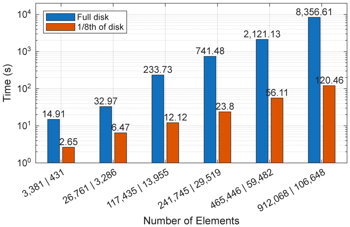
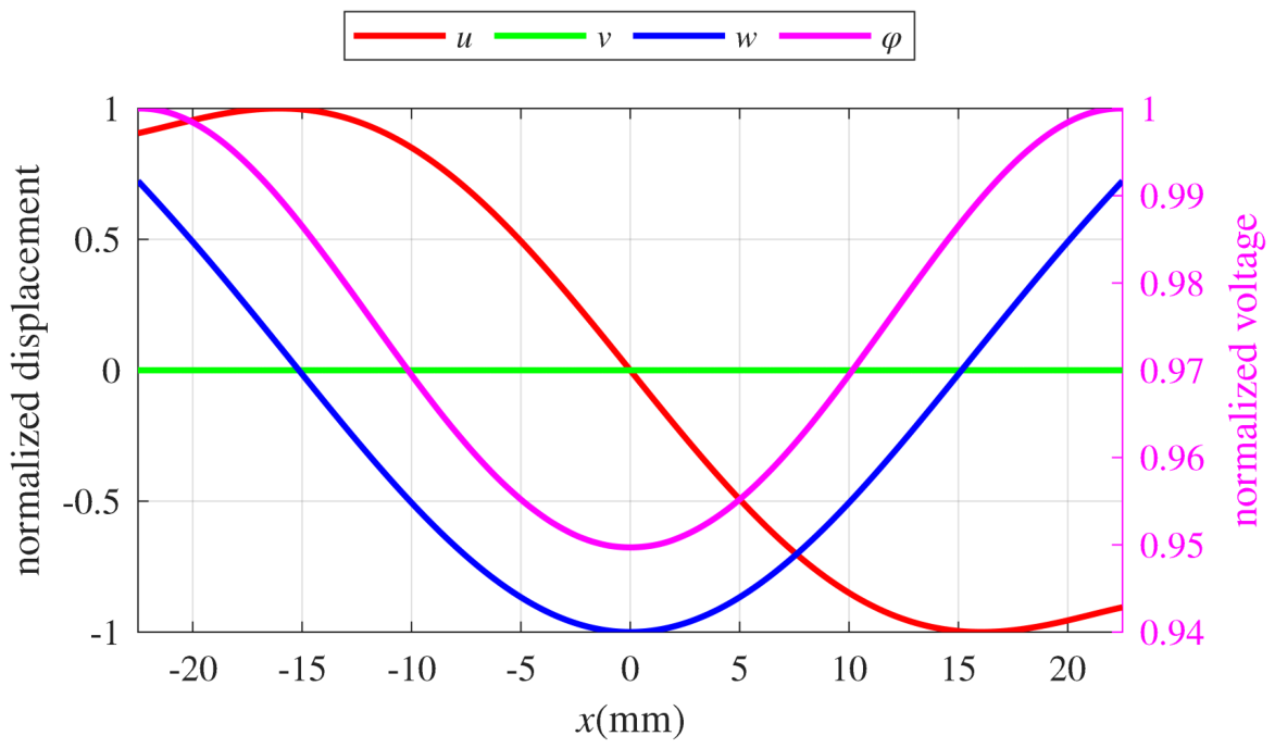
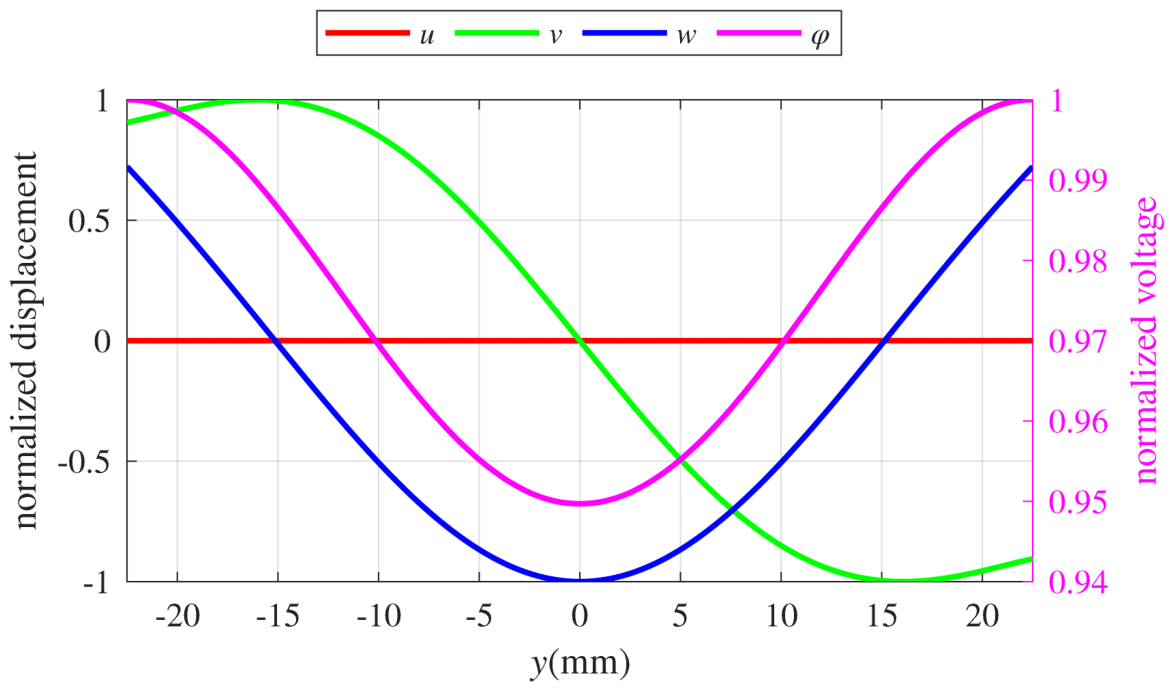
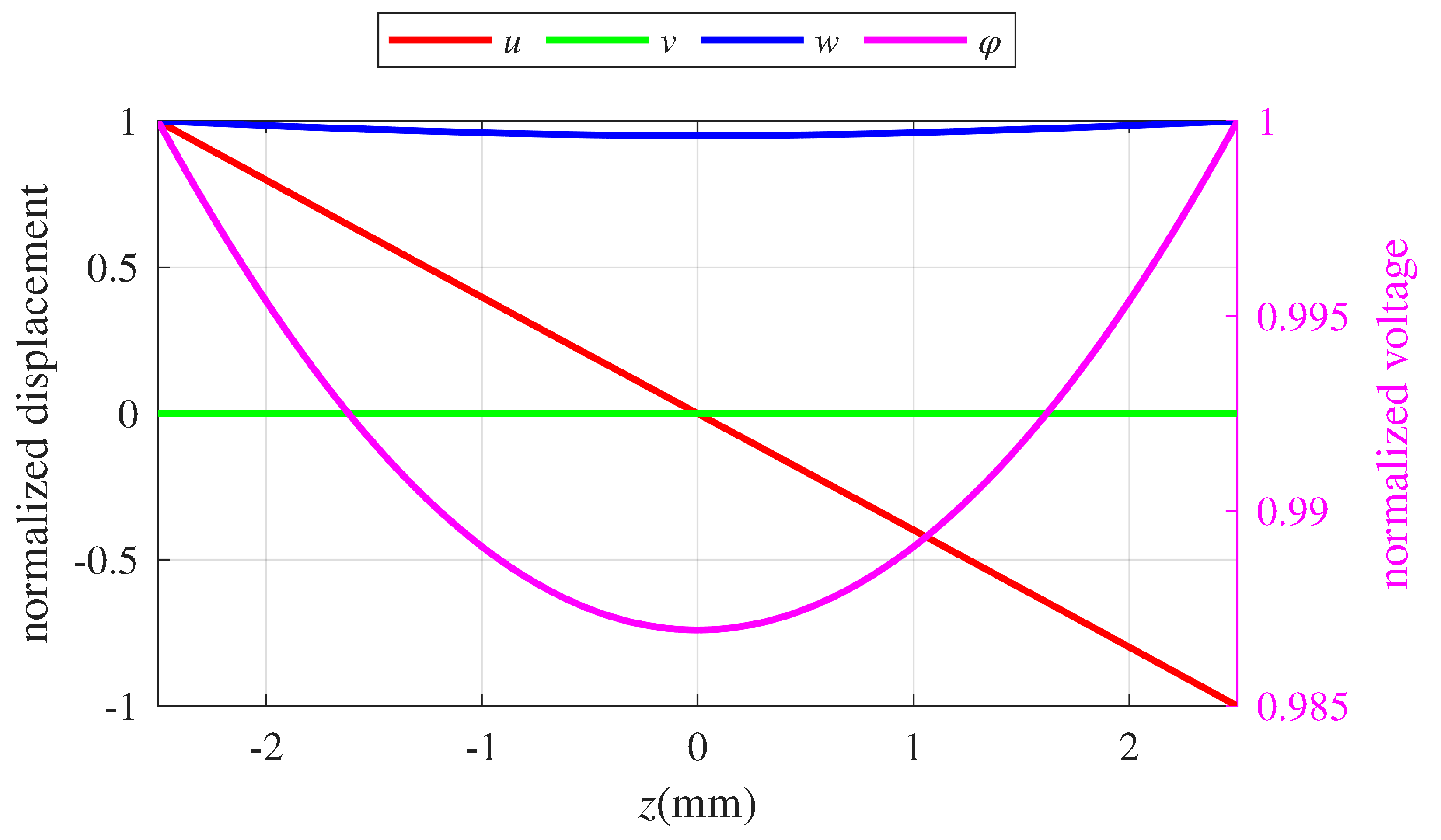
From Table 3, it can be seen that by applying the respective boundary conditions to 1/8th of the model, all the modes of the full model were obtained and classified into their respective symmetries. Also, from Figure 1, it can be seen that the 1/8th model proved to be up to 69 times faster. The time used by the 1/8th model increases a lot slower than that for the full model, which allows for more element density without sacrificing time and accuracy. To further test S 3 symmetry, plots of the Degrees Of Freedom (DOFs) at the first standalone mode (no doublets; doublets are also commonly known as degenerate modes) along lines parallel to the principal axis were made, as shown in Figure 2, Figure 3 and Figure 4. These graphs are taken from the full disk model. It is important to note that they follow S 3 parity conditions from Table 1 even though the S 3 boundary conditions from Table 2 were not applied to this model.
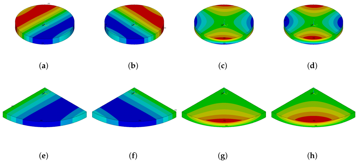
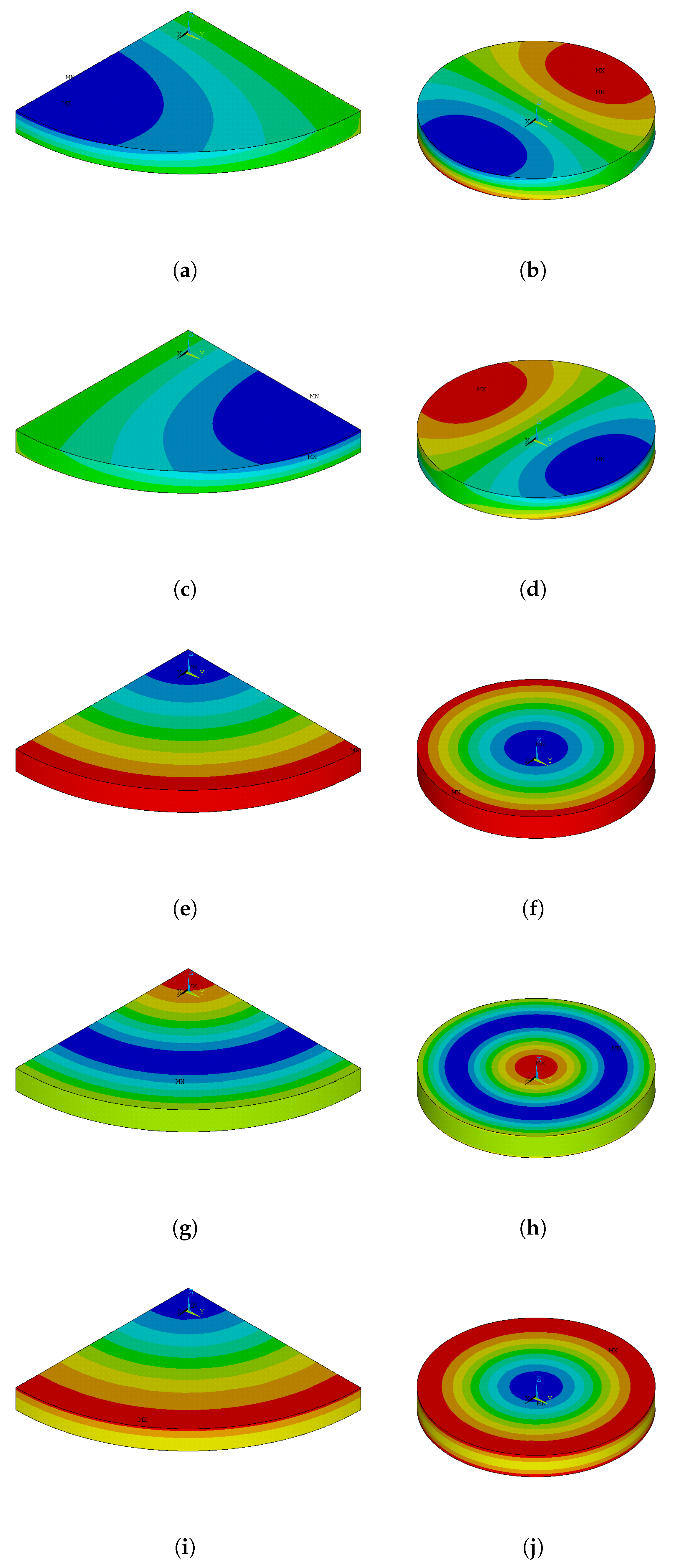
Lastly, to graphically compare the 1/8th model with the full disk model, contour plots of the DOFs were made, as shown in Figure 5. It can be seen that the 1/8th model closely resembles the full model. Similar analyses were made for the other seven symmetries by applying their respective boundary conditions shown in Appendix D, which allowed us to classify the modes of vibration. To further explore these symmetries, in the following section, they were applied to a piezoelectric ring to see how varying the external diameter has an impact on their natural frequencies.

4. Symmetry Applied to Piezoelectric Rings with a Varying External Diameter

The aim of this section, besides testing the symmetries in another common geometry, is to test how varying the external diameter affects natural frequencies. To achieve this first, we performed several modal analyses of a piezoelectric ring of PZT-8 material, with a fixed internal diameter of 15 mm and a thickness of 5 mm (these measures were chosen because they model the real ring discussed in the following sections) at an external diameter varying from 20 mm to 45 mm. Then, we proceeded to do the same for 1/8th of the disk but applied each of the eight symmetry conditions and compared them. Lastly, a comparison between the symmetries, highlighting the most important findings, is presented.
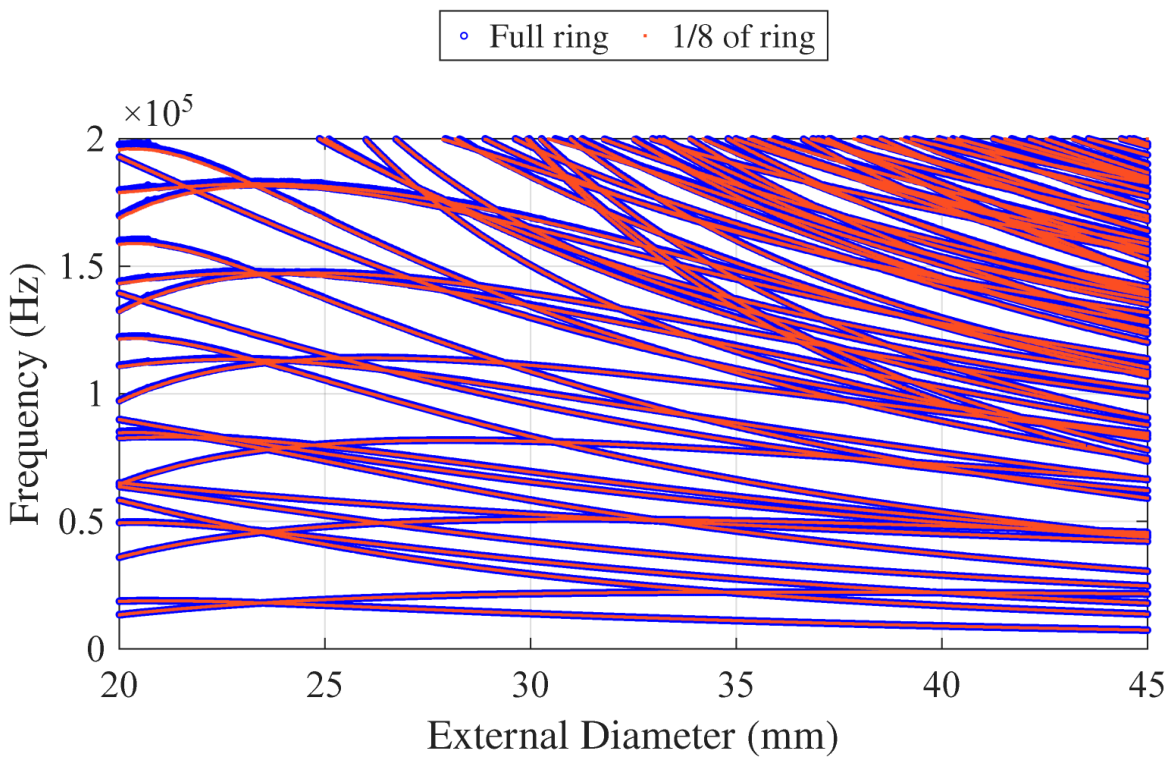
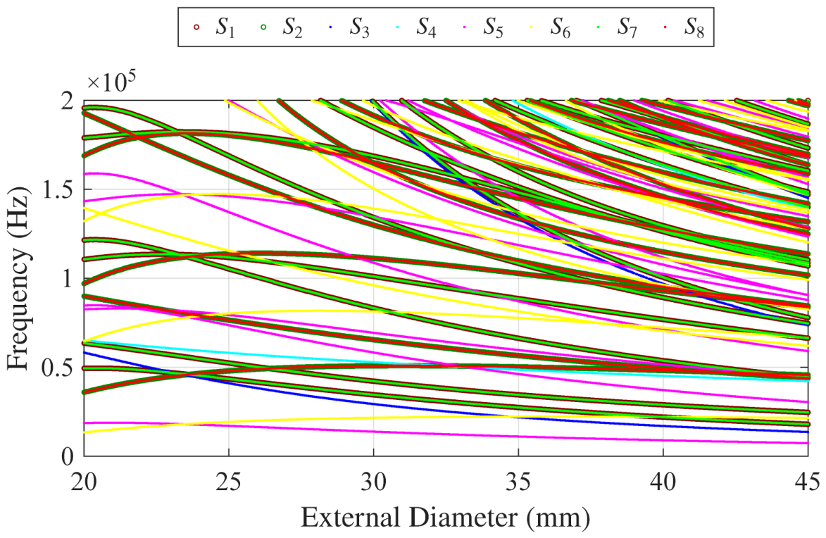
First, we can see a comparison between the full ring and 1/8th of the ring in Figure 6. Here it is important to note that every mode of the full ring is followed by a mode in 1/8th of the model. A plot classifying each of the eight symmetries is presented in Figure 7. These plots were made by performing modal analyses in 1/8th of the whole ring and applying the respective boundary conditions.
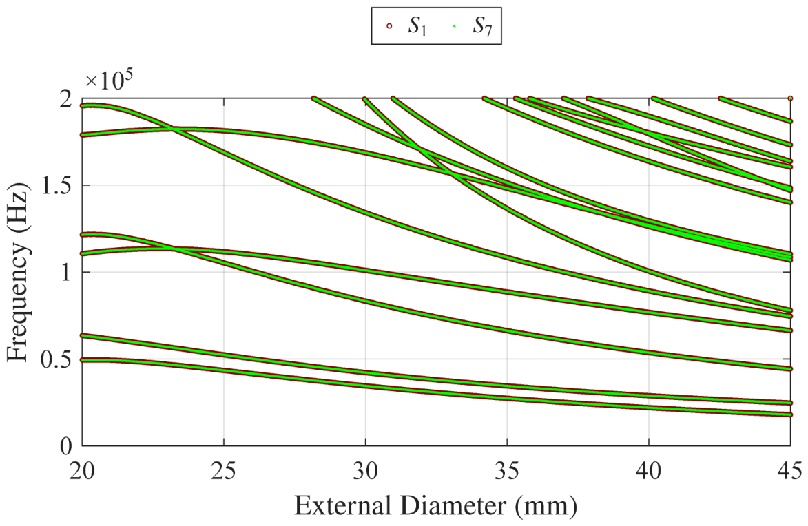
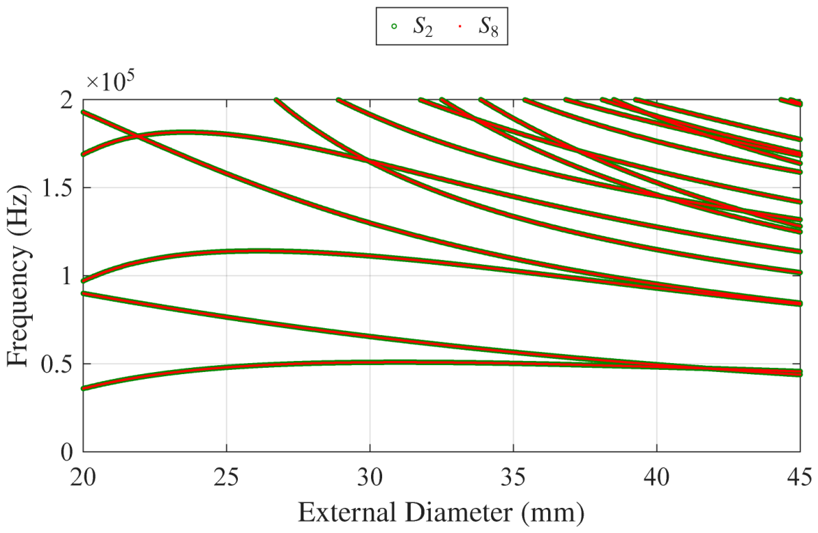
Then, from Figure 7, we isolate S 1 and S 7 and compare them in Figure 8, as well as S 2 and S 8 in Figure 9. From these plots, one can infer that S 1 = S 7 and S 2 = S 8 , and this is indeed true. One can prove this by looking at a crystal of hexagonal symmetry, as it has the same constitutive properties in the x and y directions. So, as long as the geometry is symmetrical in the x and y directions, one can interchange x with y and u with v at the same time, yielding the same system. This explains one of the many reasons why this system has several doublets. Hence, it can be said that the system has eight total symmetries that can be reduced to six. For example, in the case of an ellipsoidal prism, these eight symmetries cannot be reduced, and the doublets due to S 1 and S 7 separate, as well as the doublets due to S 2 and S 8 .
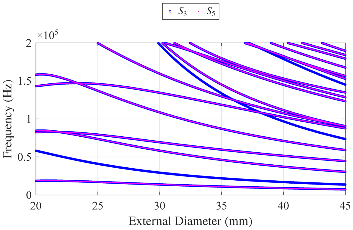
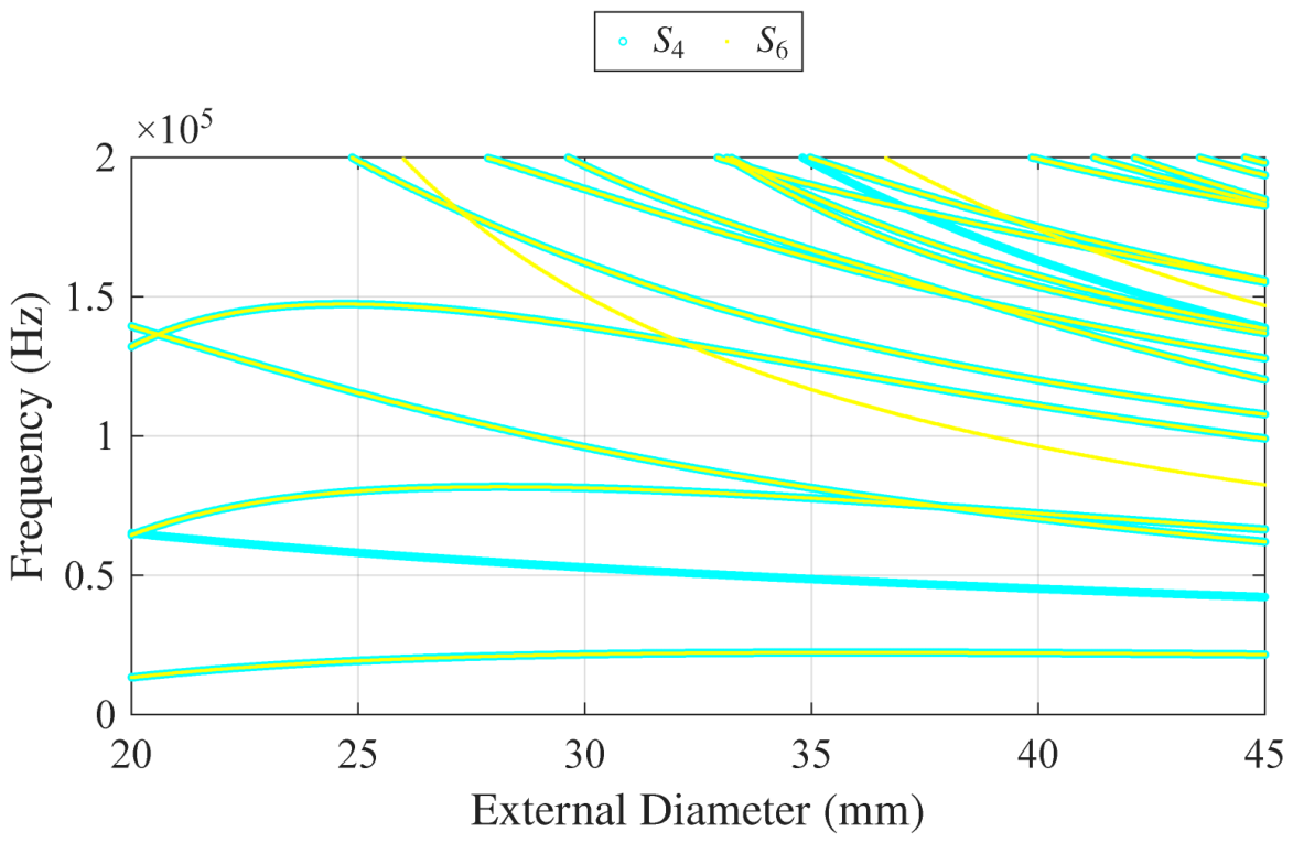
Lastly, from Figure 7, we isolate S 3 and S 5 and compare them in Figure 10, as well as S 4 and S 6 in Figure 11. Here, in both figures, it can be seen that they have several modes in common (doublets), but they also present unique modes corresponding to each symmetry. So, in this symmetry, they cannot be reduced.

5. Experimental Setup

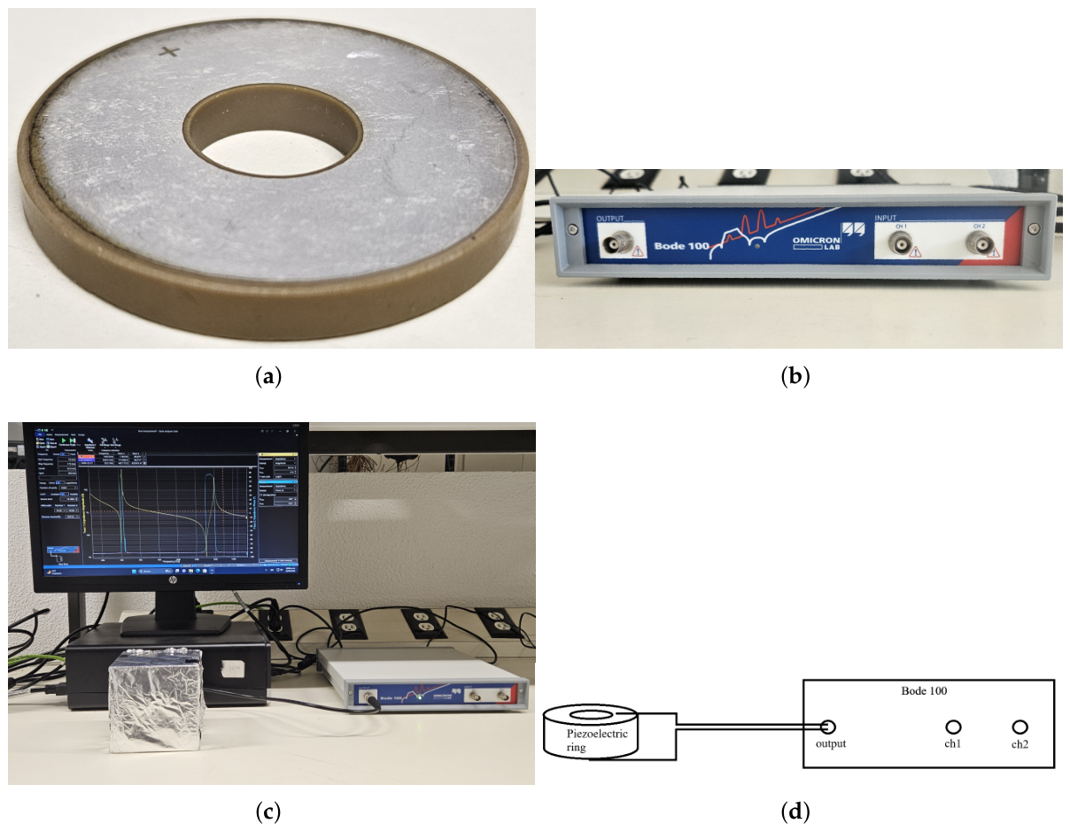
A VNA was used to measure the impedance of the piezoelectric rings while reducing their diameter to see how it affects certain resonance frequencies. We started with a piezoelectric ring of PZT-8 material, as seen in Figure 12a, with an initial outer diameter of 45 mm, an inner diameter of 15 mm and a thickness of 5 mm. Then, we proceeded to reduce its outer diameter by approximately 1 mm each time up to 31 mm and measure its impedance while following resonances.
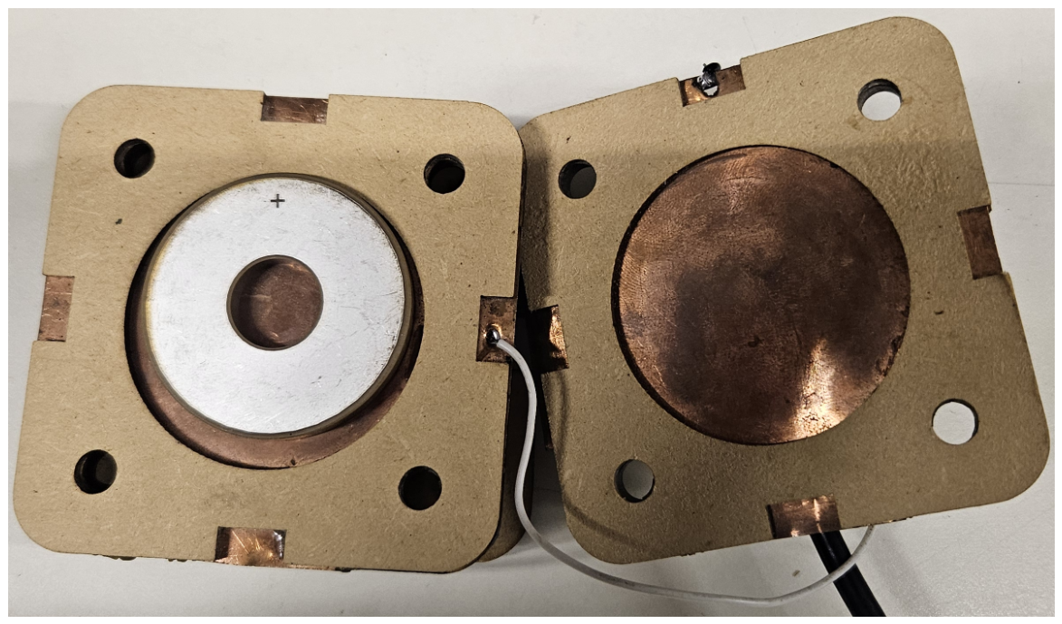
The VNA used was the Bode 100 from OMICRON Lab, shown in Figure 12b. It uses a sinusoidal waveform with a frequency range of 1 Hz to 50 MHz. The output level was set to 13 dB to reduce external noise as much as possible, which translates to 1 Vrms, as was used with the 50 Ω load. Impedance analysis was performed in the range of 10 kHz to 500 kHz with a step of 10 Hz, with a receiver bandwidth of 300 Hz. To get more accurate results, we measured the impedance six times and averaged the measurements; this helped reduce the noise in the measurements. As the aim is to measure the piezoelectric ring free of any external load (mechanical or electrical), we laid the piezoelectric ring between two copper plates, only ensuring contact, Figure 13.
To precisely reduce the outer diameter, a lathe was used by carefully sanding down each piezoelectric ring until the desired dimensions were reached. To ensure it was correctly smoothed down, a digital vernier of a standard precision of 0.02 mm was used, yielding the measurements shown in Table 4.

6. Experimental and Numerical Results

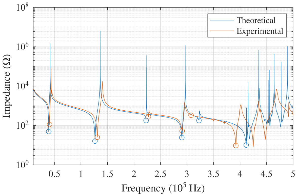
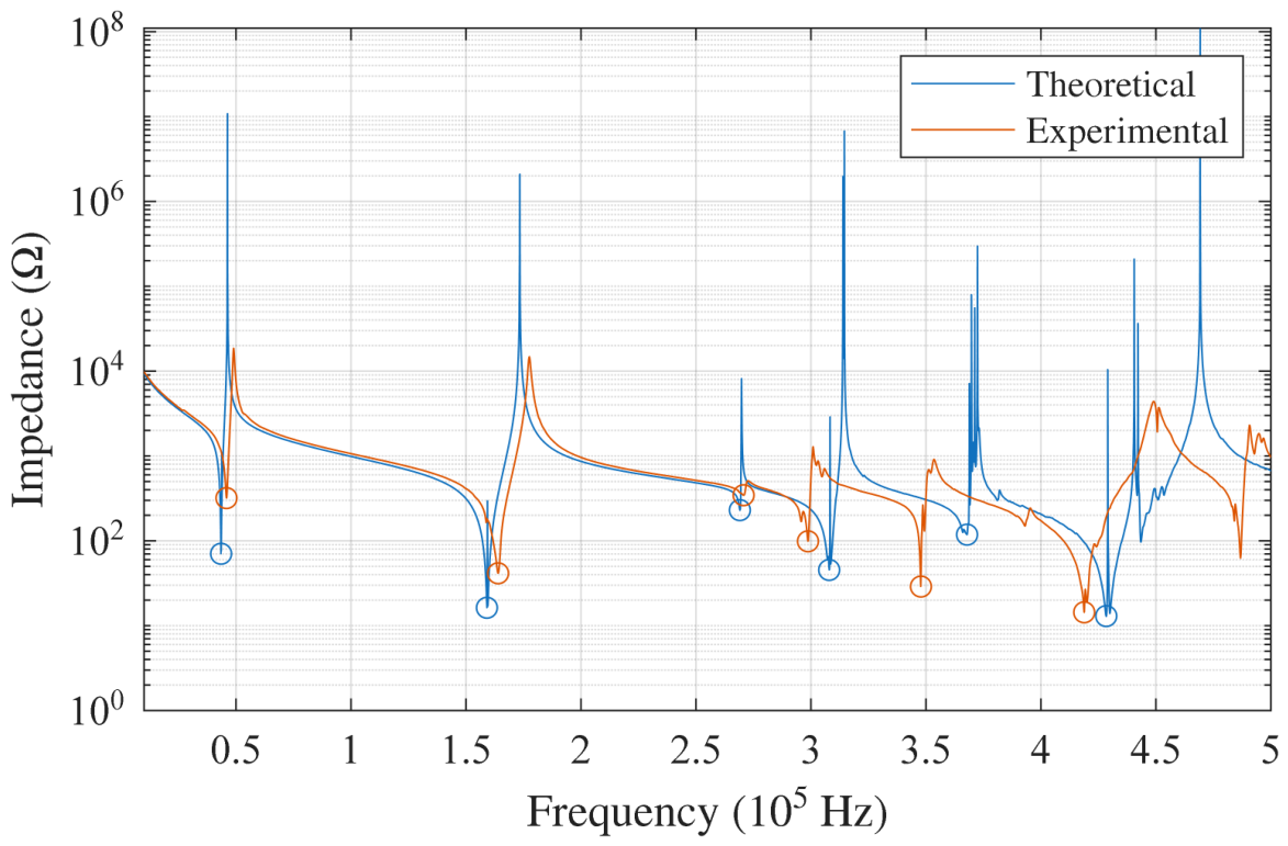
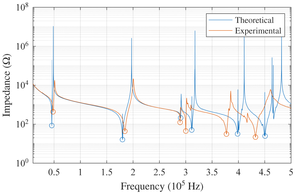
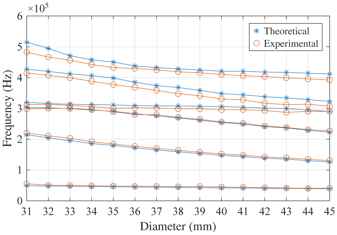
Based on the measured outer diameters in Table 4, we performed a harmonic analysis using the same frequency range of 10 kHz to 500 kHz with a step of 10 Hz. Then, we compared the results, which can be seen in Figure 14, Figure 15 and Figure 16. We tracked highlighted resonances while reducing the diameter, yielding Table 5. Then, we proceeded to plot them vs. the outer diameter, resulting in Figure 17. From Table 5, the relative percentage error was calculated for each resonance, yielding Table 6.
From Figure 17, it can be seen that the theoretical model was able to capture the general trends in the highlighted resonances, but as the frequency gets bigger, so does the error, and this model would prove unreliable after 500 kHz. From Table 5, it can be observed that after f 3 , the model tends to underestimate resonances. Also according to Table 6, f 3 seems to be the resonance at which in general the relative error ε f i tends to be minimal.

7. Conclusions

All in all, this work was able to prove that using symmetry in cylindrical geometries is not only feasible but desirable for computing efficiency. This text was able to provide a simple mathematical approach to symmetry in piezoelectric rings of class 6 mm based on function parities. The symmetries helped us model the behavior of piezoelectric rings with a varying diameter, and similar behavior appeared when performing experiments. When performing modal analysis on the piezoelectric ring with a varying diameter, two important facts stood out, S 1 = S 7 and S 2 = S 8 , which allowed us to further reduce the symmetries. One of the main limitations of this work can be found in symmetries S 3 and S 5 as well as in S 4 and S 6 ; they share natural frequencies but are not exactly the same, which suggests a further reduction in the symmetries or a possibility for a more concise symmetry description that can limit the doublets further and consequently decrease the computational cost. The other main limitation can be found in the experimental vs. numerical results when performing harmonic analysis. The numerical model represents the general behavior in terms of the shift in resonances, but this numerical model can and should be further improved to closely model the experimental data. Even though in our experiments, the temperature was not measured, it is well known that one of the causes of the shifting in frequencies is temperature. Furthermore, the elastic, piezoelectric, and dielectric properties of the PZT-8 material are reported with an error; this can also shift frequency. For this reason, future work should aim to perform optimization to adjust the experimental and numerical results. This will allow us to characterize piezoelectrics and thus further improve the model.

Author Contributions

A.A.N.M.: Conceptualization (equal), data curation, investigation, methodology (equal), resources (equal), software, validation (equal), writing—original draft, writing—review and editing (equal). J.E.C.Q.: Project administration (equal), resources (equal), supervision (equal), writing—review and editing (equal). J.A.O.: Conceptualization (equal), methodology (equal), project administration (equal), resources (equal), supervision (equal), validation (equal), writing—review and editing (equal). All authors have read and agreed to the published version of the manuscript.

Funding

This research received no external funding.

Institutional Review Board Statement

Not applicable.

Informed Consent Statement

Not applicable.

Data Availability Statement

The data that support the findings of this study are available from the corresponding author upon reasonable request.

Acknowledgments

Axayácatl A. N. Montiel acknowledges SECIHTI Mexico for the Ph.D scholarship.

Conflicts of Interest

The authors declare no conflicts of interest.

Appendix A. Symmetry Conditions

In this Appendix, the rest of the eight symmetry conditions are stated. From Table A1, Table A2, Table A3, Table A4, Table A5, Table A6 and Table A7, it can be seen how the displacements and electric potential have parity conditions that complement the stress and electric displacement respectively, each along the three main axes (x, y, and z).
Table A1. S 1 symmetry condition.
PlanesDisplacements and Electric PotentialStresses and Electric Displacement
x = 0 u ( x , y , z ) = u ( x , y , z ) σ x x ( x , y , z ) = σ x x ( x , y , z )
v ( x , y , z ) = v ( x , y , z ) σ x y ( x , y , z ) = σ x y ( x , y , z )
w ( x , y , z ) = w ( x , y , z ) σ x z ( x , y , z ) = σ x z ( x , y , z )
φ ( x , y , z ) = φ ( x , y , z ) D x ( x , y , z ) = D x ( x , y , z )
y = 0 u ( x , y , z ) = u ( x , y , z ) σ y x ( x , y , z ) = σ y x ( x , y , z )
v ( x , y , z ) = v ( x , y , z ) σ y y ( x , y , z ) = σ y y ( x , y , z )
w ( x , y , z ) = w ( x , y , z ) σ y z ( x , y , z ) = σ y z ( x , y , z )
φ ( x , y , z ) = φ ( x , y , z ) D y ( x , y , z ) = D y ( x , y , z )
z = 0 u ( x , y , z ) = u ( x , y , z ) σ z x ( x , y , z ) = σ z x ( x , y , z )
v ( x , y , z ) = v ( x , y , z ) σ z y ( x , y , z ) = σ z y ( x , y , z )
w ( x , y , z ) = w ( x , y , z ) σ z z ( x , y , z ) = σ z z ( x , y , z )
φ ( x , y , z ) = φ ( x , y , z ) D z ( x , y , z ) = D z ( x , y , z )
Table A2. S 2 symmetry condition.
PlanesDisplacements and Electric PotentialStresses and Electric Displacement
x = 0 u ( x , y , z ) = u ( x , y , z ) σ x x ( x , y , z ) = σ x x ( x , y , z )
v ( x , y , z ) = v ( x , y , z ) σ x y ( x , y , z ) = σ x y ( x , y , z )
w ( x , y , z ) = w ( x , y , z ) σ x z ( x , y , z ) = σ x z ( x , y , z )
φ ( x , y , z ) = φ ( x , y , z ) D x ( x , y , z ) = D x ( x , y , z )
y = 0 u ( x , y , z ) = u ( x , y , z ) σ y x ( x , y , z ) = σ y x ( x , y , z )
v ( x , y , z ) = v ( x , y , z ) σ y y ( x , y , z ) = σ y y ( x , y , z )
w ( x , y , z ) = w ( x , y , z ) σ y z ( x , y , z ) = σ y z ( x , y , z )
φ ( x , y , z ) = φ ( x , y , z ) D y ( x , y , z ) = D y ( x , y , z )
z = 0 u ( x , y , z ) = u ( x , y , z ) σ z x ( x , y , z ) = σ z x ( x , y , z )
v ( x , y , z ) = v ( x , y , z ) σ z y ( x , y , z ) = σ z y ( x , y , z )
w ( x , y , z ) = w ( x , y , z ) σ z z ( x , y , z ) = σ z z ( x , y , z )
φ ( x , y , z ) = φ ( x , y , z ) D z ( x , y , z ) = D z ( x , y , z )
Table A3. S 4 symmetry condition.
PlanesDisplacements and Electric PotentialStresses and Electric Displacement
x = 0 u ( x , y , z ) = u ( x , y , z ) σ x x ( x , y , z ) = σ x x ( x , y , z )
v ( x , y , z ) = v ( x , y , z ) σ x y ( x , y , z ) = σ x y ( x , y , z )
w ( x , y , z ) = w ( x , y , z ) σ x z ( x , y , z ) = σ x z ( x , y , z )
φ ( x , y , z ) = φ ( x , y , z ) D x ( x , y , z ) = D x ( x , y , z )
y = 0 u ( x , y , z ) = u ( x , y , z ) σ y x ( x , y , z ) = σ y x ( x , y , z )
v ( x , y , z ) = v ( x , y , z ) σ y y ( x , y , z ) = σ y y ( x , y , z )
w ( x , y , z ) = w ( x , y , z ) σ y z ( x , y , z ) = σ y z ( x , y , z )
φ ( x , y , z ) = φ ( x , y , z ) D y ( x , y , z ) = D y ( x , y , z )
z = 0 u ( x , y , z ) = u ( x , y , z ) σ z x ( x , y , z ) = σ z x ( x , y , z )
v ( x , y , z ) = v ( x , y , z ) σ z y ( x , y , z ) = σ z y ( x , y , z )
w ( x , y , z ) = w ( x , y , z ) σ z z ( x , y , z ) = σ z z ( x , y , z )
φ ( x , y , z ) = φ ( x , y , z ) D z ( x , y , z ) = D z ( x , y , z )
Table A4. S 5 symmetry condition.
PlanesDisplacements and Electric PotentialStresses and Electric Displacement
x = 0 u ( x , y , z ) = u ( x , y , z ) σ x x ( x , y , z ) = σ x x ( x , y , z )
v ( x , y , z ) = v ( x , y , z ) σ x y ( x , y , z ) = σ x y ( x , y , z )
w ( x , y , z ) = w ( x , y , z ) σ x z ( x , y , z ) = σ x z ( x , y , z )
φ ( x , y , z ) = φ ( x , y , z ) D x ( x , y , z ) = D x ( x , y , z )
y = 0 u ( x , y , z ) = u ( x , y , z ) σ y x ( x , y , z ) = σ y x ( x , y , z )
v ( x , y , z ) = v ( x , y , z ) σ y y ( x , y , z ) = σ y y ( x , y , z )
w ( x , y , z ) = w ( x , y , z ) σ y z ( x , y , z ) = σ y z ( x , y , z )
φ ( x , y , z ) = φ ( x , y , z ) D y ( x , y , z ) = D y ( x , y , z )
z = 0 u ( x , y , z ) = u ( x , y , z ) σ z x ( x , y , z ) = σ z x ( x , y , z )
v ( x , y , z ) = v ( x , y , z ) σ z y ( x , y , z ) = σ z y ( x , y , z )
w ( x , y , z ) = w ( x , y , z ) σ z z ( x , y , z ) = σ z z ( x , y , z )
φ ( x , y , z ) = φ ( x , y , z ) D z ( x , y , z ) = D z ( x , y , z )
Table A5. S 6 symmetry condition.
PlanesDisplacements and Electric PotentialStresses and Electric Displacement
x = 0 u ( x , y , z ) = u ( x , y , z ) σ x x ( x , y , z ) = σ x x ( x , y , z )
v ( x , y , z ) = v ( x , y , z ) σ x y ( x , y , z ) = σ x y ( x , y , z )
w ( x , y , z ) = w ( x , y , z ) σ x z ( x , y , z ) = σ x z ( x , y , z )
φ ( x , y , z ) = φ ( x , y , z ) D x ( x , y , z ) = D x ( x , y , z )
y = 0 u ( x , y , z ) = u ( x , y , z ) σ y x ( x , y , z ) = σ y x ( x , y , z )
v ( x , y , z ) = v ( x , y , z ) σ y y ( x , y , z ) = σ y y ( x , y , z )
w ( x , y , z ) = w ( x , y , z ) σ y z ( x , y , z ) = σ y z ( x , y , z )
φ ( x , y , z ) = φ ( x , y , z ) D y ( x , y , z ) = D y ( x , y , z )
z = 0 u ( x , y , z ) = u ( x , y , z ) σ z x ( x , y , z ) = σ z x ( x , y , z )
v ( x , y , z ) = v ( x , y , z ) σ z y ( x , y , z ) = σ z y ( x , y , z )
w ( x , y , z ) = w ( x , y , z ) σ z z ( x , y , z ) = σ z z ( x , y , z )
φ ( x , y , z ) = φ ( x , y , z ) D z ( x , y , z ) = D z ( x , y , z )
Table A6. S 7 symmetry condition.
PlanesDisplacements and Electric PotentialStresses and Electric Displacement
x = 0 u ( x , y , z ) = u ( x , y , z ) σ x x ( x , y , z ) = σ x x ( x , y , z )
v ( x , y , z ) = v ( x , y , z ) σ x y ( x , y , z ) = σ x y ( x , y , z )
w ( x , y , z ) = w ( x , y , z ) σ x z ( x , y , z ) = σ x z ( x , y , z )
φ ( x , y , z ) = φ ( x , y , z ) D x ( x , y , z ) = D x ( x , y , z )
y = 0 u ( x , y , z ) = u ( x , y , z ) σ y x ( x , y , z ) = σ y x ( x , y , z )
v ( x , y , z ) = v ( x , y , z ) σ y y ( x , y , z ) = σ y y ( x , y , z )
w ( x , y , z ) = w ( x , y , z ) σ y z ( x , y , z ) = σ y z ( x , y , z )
φ ( x , y , z ) = φ ( x , y , z ) D y ( x , y , z ) = D y ( x , y , z )
z = 0 u ( x , y , z ) = u ( x , y , z ) σ z x ( x , y , z ) = σ z x ( x , y , z )
v ( x , y , z ) = v ( x , y , z ) σ z y ( x , y , z ) = σ z y ( x , y , z )
w ( x , y , z ) = w ( x , y , z ) σ z z ( x , y , z ) = σ z z ( x , y , z )
φ ( x , y , z ) = φ ( x , y , z ) D z ( x , y , z ) = D z ( x , y , z )
Table A7. S 8 symmetry condition.
PlanesDisplacements and Electric PotentialStresses and Electric Displacement
x = 0 u ( x , y , z ) = u ( x , y , z ) σ x x ( x , y , z ) = σ x x ( x , y , z )
v ( x , y , z ) = v ( x , y , z ) σ x y ( x , y , z ) = σ x y ( x , y , z )
w ( x , y , z ) = w ( x , y , z ) σ x z ( x , y , z ) = σ x z ( x , y , z )
φ ( x , y , z ) = φ ( x , y , z ) D x ( x , y , z ) = D x ( x , y , z )
y = 0 u ( x , y , z ) = u ( x , y , z ) σ y x ( x , y , z ) = σ y x ( x , y , z )
v ( x , y , z ) = v ( x , y , z ) σ y y ( x , y , z ) = σ y y ( x , y , z )
w ( x , y , z ) = w ( x , y , z ) σ y z ( x , y , z ) = σ y z ( x , y , z )
φ ( x , y , z ) = φ ( x , y , z ) D y ( x , y , z ) = D y ( x , y , z )
z = 0 u ( x , y , z ) = u ( x , y , z ) σ z x ( x , y , z ) = σ z x ( x , y , z )
v ( x , y , z ) = v ( x , y , z ) σ z y ( x , y , z ) = σ z y ( x , y , z )
w ( x , y , z ) = w ( x , y , z ) σ z z ( x , y , z ) = σ z z ( x , y , z )
φ ( x , y , z ) = φ ( x , y , z ) D z ( x , y , z ) = D z ( x , y , z )

Appendix B. Boundary Conditions by Symmetry of 1/8th of Disk

In this Appendix, the rest of the eight boundary conditions by symmetry to be applied to 1/8th of the disk are stated through Table A8, Table A9, Table A10, Table A11, Table A12, Table A13 and Table A14. Each table presents the boundary conditions to be applied to 1/8th of the disk at the principal planes ( x = 0 , y = 0 , and z = 0 ) for each symmetry.
Table A8. S 1 boundary conditions of 1/8th of disk.
PlanesBoundary Conditions
x = 0 u = 0 ,   σ x y = 0 ,   σ x z = 0 ,   D x = 0
y = 0 u = 0 ,   σ y y = 0 ,   w = 0 ,   φ = 0
z = 0 u = 0 ,   v = 0 ,   σ z z = 0 ,   D z = 0
Table A9. S 2 boundary conditions of 1/8th of disk.
PlanesBoundary Conditions
x = 0 u = 0 ,   σ x y = 0 ,   σ x z = 0 ,   D x = 0
y = 0 u = 0 ,   σ y y = 0 ,   w = 0 ,   φ = 0
z = 0 σ z x = 0 ,   σ z y = 0 ,   w = 0 ,   φ = 0
Table A10. S 4 boundary conditions of 1/8th of disk.
PlanesBoundary Conditions
x = 0 u = 0 ,   σ x z = 0 ,   σ x y = 0 ,   D x = 0
y = 0 σ y x = 0 ,   v = 0 ,   σ y z = 0 ,   D y = 0
z = 0 σ z x = 0 ,   σ z y = 0 ,   w = 0 ,   φ = 0
Table A11. S 5 boundary conditions of 1/8th of disk.
PlanesBoundary Conditions
x = 0 σ x x = 0 ,   v = 0 ,   w = 0 ,   φ = 0
y = 0 u = 0 ,   σ y y = 0 ,   w = 0 ,   φ = 0
z = 0 u = 0 ,   v = 0 ,   σ z z = 0 ,   D z = 0
Table A12. S 6 boundary conditions of 1/8th of disk.
PlanesBoundary Conditions
x = 0 σ x x = 0 ,   v = 0 ,   w = 0 ,   φ = 0
y = 0 u = 0 ,   σ y y = 0 ,   w = 0 ,   φ = 0
z = 0 σ z x = 0 ,   σ z y = 0 ,   w = 0 ,   φ = 0
Table A13. S 7 boundary conditions of 1/8th of disk.
PlanesBoundary Conditions
x = 0 σ x x = 0 ,   v = 0 ,   w = 0 ,   φ = 0
y = 0 σ y x = 0 ,   v = 0 ,   σ y z = 0 ,   D y = 0
z = 0 u = 0 ,   v = 0 ,   σ z z = 0 ,   D z = 0
Table A14. S 8 boundary conditions of 1/8th of disk.
PlanesBoundary Conditions
x = 0 σ x x = 0 ,   v = 0 ,   w = 0 ,   φ = 0
y = 0 σ y x = 0 ,   v = 0 ,   σ y z = 0 ,   D y = 0
z = 0 σ z x = 0 ,   σ z y = 0 ,   w = 0 ,   φ = 0

Appendix C. Mesh Convergence Study for Whole Disk

In this Appendix, the mesh convergence study for the modal analysis of a piezoelectric disk is presented. The piezoelectric disk was made of PZT-8 material, with a 45 mm outer diameter and a thickness of 5 mm. In Table A15 and Table A16, the number of elements is increased from left to right and from Table A15 to Table A16. It can be seen that the values of the natural frequencies along with their doublets converge as the number of elements increases.
Table A15. Mesh convergence analysis for modal analysis of whole disk.
ModeFrequency (kHz)
with
3381 Elements
Frequency (kHz)
with
26,761 Elements
Frequency (kHz)
with
117,435 Elements
18.2516187298.2449070298.244326435
28.2524899048.2450228738.244335603
315.8000924515.7923258915.7909633
418.3717573418.3366678618.33350837
518.3723928318.3369155318.33351935
630.6641779830.5696302730.56056295
730.6725979130.5698409730.56068952
832.3928954932.3437963932.33590344
932.3952353632.343983332.33590799
1034.5572433734.5570689234.55705326
1134.5572486934.5570701834.55705331
1241.6633322641.6629249741.6628822
1341.6633348841.6629263641.66288224
1444.5359984844.3267975944.30802922
1544.5388043944.3278376144.3080612
Table A16. Mesh convergence analysis for continued modal analysis of whole disk.
ModeFrequency (kHz)
with
241,745 Elements
Frequency (kHz)
with
465,466 Elements
Frequency (kHz)
with
912,068 Elements
18.2442372618.244203398.244195528
28.2442382248.2442060438.244196709
315.7909008315.7908767815.79086726
418.3330772918.3329204818.33287827
518.3330795618.3329216718.33287857
630.5594593330.5590225930.55890865
730.5594635730.5590377230.55891266
832.3354610832.3352988332.33523593
932.3354613432.335299332.33523607
1034.5570518634.5570514434.55705126
1134.5570518734.5570514434.55705128
1241.6628785941.662877541.66287705
1341.6628786141.6628775141.66287706
1444.3055949444.3046765844.30441654
1544.3056106244.3046791144.30441985

Appendix D. Comparison of Contour Plots by Symmetry

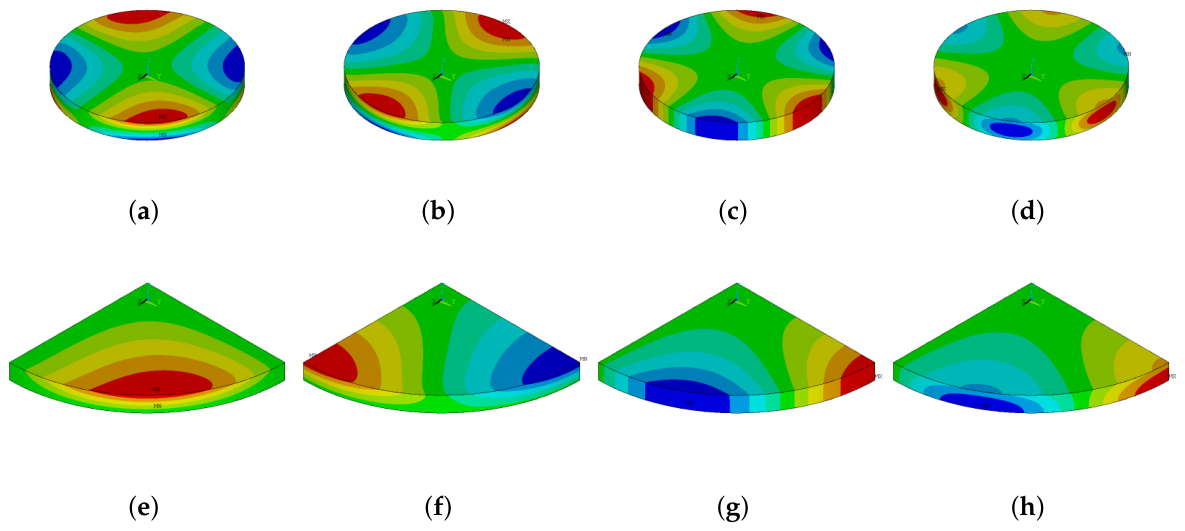
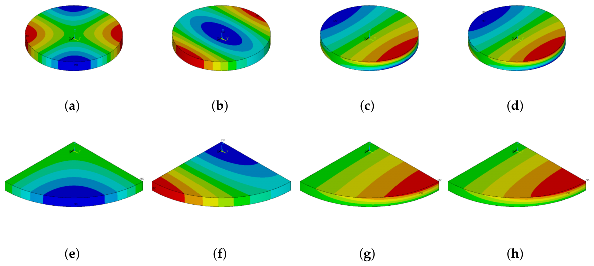
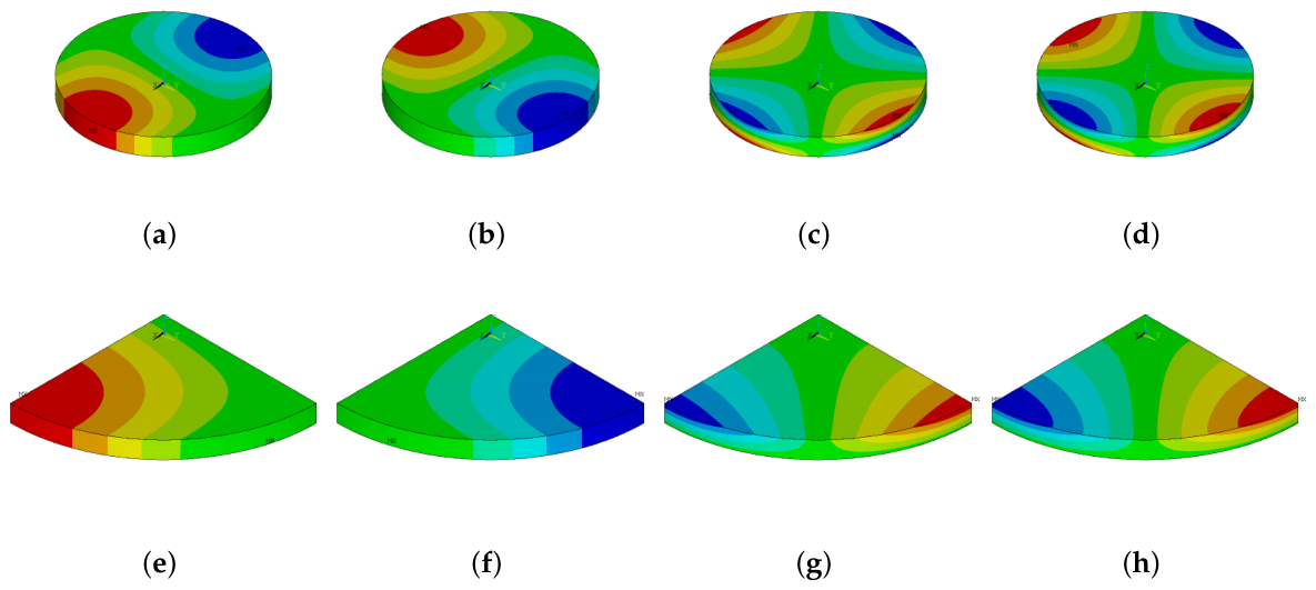
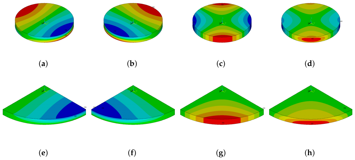
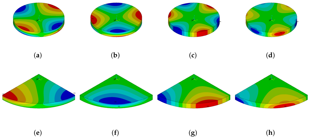
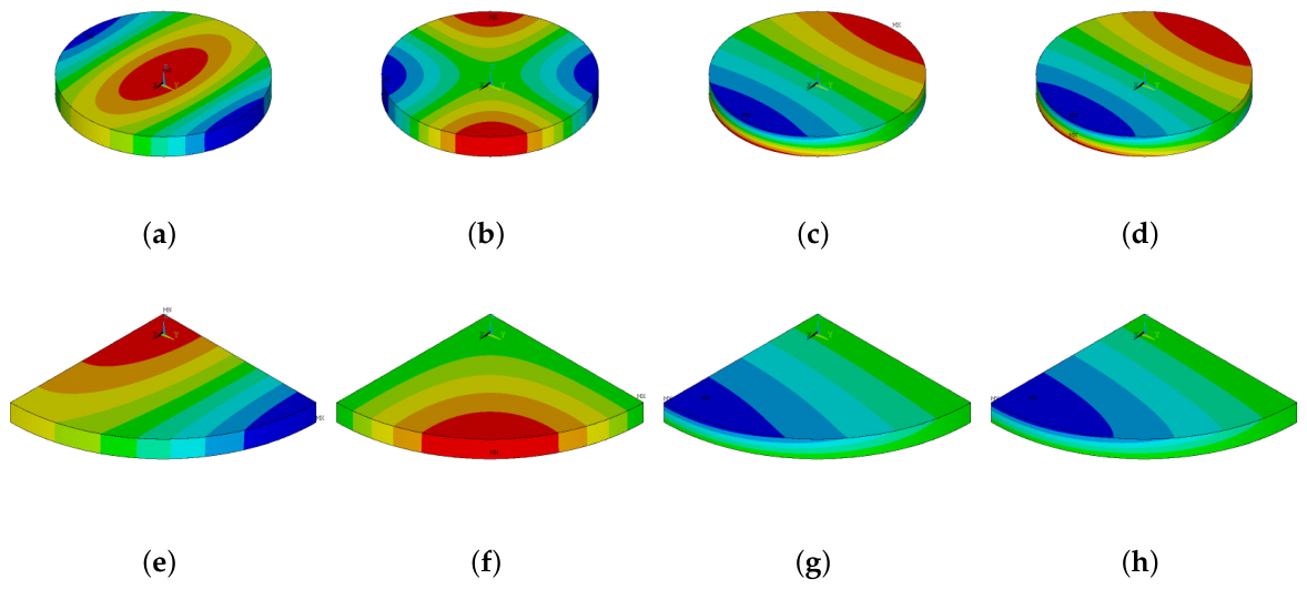
This Appendix shows contour plots for a PZT-8 piezoelectric disk of 45 mm outer diameter and 5 mm thickness. Figure A1, Figure A2, Figure A3, Figure A4, Figure A5, Figure A6 and Figure A7 compare the contour plots of the DOFs obtained with the free full model disk vs. its 1/8th model applying symmetry. Note that the S 3 contour plots are missing because they were previously displayed in this article in Figure 5.
Figure A1. A comparison of the contour plots of the DOFs, full disk vs. 1/8th respectively at 18,336 (Hz) corresponding to S 1 : (a,e) plot the displacement u; (b,f) plot the displacement v; (c,g) plot the displacement w; (d,h) plot the electric potential φ .
Applsci 16 08797 g0a1
Figure A2. A comparison of the contour plots of the DOFs, full disk vs. 1/8th respectively at 41,663 (Hz) corresponding to S 2 : (a,e) plot the displacement u; (b,f) plot the displacement v; (c,g) plot the displacement w; (d,h) plot the electric potential φ .
Applsci 16 08797 g0a2
Figure A3. A comparison of the contour plots of the DOFs, full disk vs. 1/8th respectively at 34,557 (Hz) corresponding to S 4 : (a,e) plot the displacement u; (b,f) plot the displacement v; (c,g) plot the displacement w; (d,h) plot the electric potential φ .
Applsci 16 08797 g0a3
Figure A4. A comparison of the contour plots of the DOFs, full disk vs. 1/8th respectively at 8245 (Hz) corresponding to S 5 : (a,e) plot the displacement u; (b,f) plot the displacement v; (c,g) plot the displacement w; (d,h) plot the electric potential φ .
Applsci 16 08797 g0a4
Figure A5. A comparison of the contour plots of the DOFs, full disk vs. 1/8th respectively at 34,557 (Hz) corresponding to S 6 : (a,e) plot the displacement u; (b,f) plot the displacement v; (c,g) plot the displacement w; (d,h) plot the electric potential φ .
Applsci 16 08797 g0a5
Figure A6. A comparison of the contour plots of the DOFs, full disk vs. 1/8th respectively at 18,337 (Hz) corresponding to S 7 : (a,e) plot the displacement u; (b,f) plot the displacement v; (c,g) plot the displacement w; (d,h) plot the electric potential φ .
Applsci 16 08797 g0a6
Figure A7. A comparison of the contour plots of the DOFs, full disk vs. 1/8th respectively at 41,663 (Hz) corresponding to S 8 : (a,e) plot the displacement u; (b,f) plot the displacement v; (c,g) plot the displacement w; (d,h) plot the electric potential φ .
Applsci 16 08797 g0a7

References

  1. Graff, K.F. (Ed.) Power Ultrasonics; Elsevier Science: Oxford, UK, 2014. [Google Scholar]
  2. Rahaman, A.; Kim, B.; Park, D. Design and characterizations of a multi–sound receiver using fly Ormia ochracea’s ears–inspired MEMS directional microphone array. Appl. Acoust. 2025, 228, 110359. [Google Scholar] [CrossRef] [Scilit]
  3. Joshan, Y.S.; Santapuri, S.; Srinivasa, A. Finite element modeling and analysis of low symmetry piezoelectric shells for design of shear sensors. Int. J. Mech. Sci. 2021, 210, 106726. [Google Scholar] [CrossRef] [Scilit]
  4. Ju, M.; Dou, Z.; Li, J.W.; Qiu, X.; Shen, B.; Zhang, D.; Yao, F.Z.; Gong, W.; Wang, K. Piezoelectric Materials and Sensors for Structural Health Monitoring: Fundamental Aspects, Current Status, and Future Perspectives. Sensors 2023, 23, 543. [Google Scholar] [CrossRef] [Scilit]
  5. Zhang, X.; Liang, B. Piezoelectric ultrasonic transducer for longitudinal-flexural vibrational mode-conversion. Appl. Acoust. 2018, 129, 284–290. [Google Scholar] [CrossRef] [Scilit]
  6. Neary, B.; Butan, D.; MacLoughlin, R.; Griffin, P. Finite Element Analysis of Active Vibrating Mesh Nebulisers and Atomisers for Respiratory Drug Delivery—A Review. Appl. Sci. 2026, 16, 4796. [Google Scholar] [CrossRef] [Scilit]
  7. Delibas, B.; Koc, B. Single crystal piezoelectric motor operating with both inertia and ultrasonic resonance drives. Ultrasonics 2024, 136, 107140. [Google Scholar] [CrossRef] [Scilit]
  8. Dou, Z.; Da, J.; Zhou, G.; Zhang, S.; Chen, W.; Yang, Y.; Yan, H.; Liu, F. Study on the Growth and Desorption of Lubricating Oil Droplets in Space Under Piezoelectric Drive. Appl. Sci. 2026, 16, 2449. [Google Scholar] [CrossRef] [Scilit]
  9. Uchino, K. Piezoelectric ultrasonic motors: Overview. Smart Mater. Struct. 1998, 7, 273. [Google Scholar] [CrossRef] [Scilit]
  10. Wang, Y.; Gong, J.; Gao, T.; Wu, M.; Wu, X.; Lu, C.; He, W. The influence of aspect ratio on coupled mode vibration in rectangular piezoelectric resonators: A finite element and mechanistic analysis. Appl. Acoust. 2026, 253, 111389. [Google Scholar] [CrossRef] [Scilit]
  11. Xu, J.; Zhang, Y.; Negahban, M.; Shao, S.; Wang, W.; Li, Z. A tunable piezoelectric metasurface ring for wave manipulation and vibration isolation in cylindrical shells. Thin-Walled Struct. 2026, 230, 115324. [Google Scholar] [CrossRef] [Scilit]
  12. Liu, L.; Zhang, Y.; Sun, Y.; Wang, J.; Gao, W.; Wu, F.; Chang, Y.; Yang, B.; Chi, Q. Significantly enhanced strain and low hysteresis of synergistic designed textured ceramics for piezoelectric actuators. Ceram. Int. 2026, 52, 34886–34893. [Google Scholar] [CrossRef] [Scilit]
  13. Tang, C.; Yu, L.; Fang, W.; Liu, P.; Wang, S.; Kan, J.; Zhang, Z. A wideband piezoelectric-electromagnetic hybrid rotational energy harvester with excited-magnet-detached piezoelectric transducer and magnet-built-in coil. Sustain. Energy Technol. Assess. 2026, 91, 105067. [Google Scholar] [CrossRef] [Scilit]
  14. Bakhtiar, S.; Masabi, S.N.; Li, T.; Papuga, J.; West, A.; Jiang, J.; Theodossiades, S. Energy Harvesting from Clustered Piezoelectric Beams for Aircraft Health Monitoring Systems. Appl. Sci. 2026, 16, 3115. [Google Scholar] [CrossRef] [Scilit]
  15. Zhang, E.; Li, Z.; Suo, L.; Wang, D.; Zhang, X. High-performance piezoelectric metamaterial design for energy harvesting. Thin-Walled Struct. 2026, 228, 115121. [Google Scholar] [CrossRef] [Scilit]
  16. Liu, Z.; Wang, X.; Yang, D.; Tian, D.; Liu, X.; Li, Y.; Duan, X.; Zhao, X.; Yu, F. Ultrahigh-temperature piezoelectric crystal ErxGd1−xCa40BO33 with near-zero temperature-shift of piezoelectric properties. J. Mater. 2026, 12, 101259. [Google Scholar] [CrossRef] [Scilit]
  17. Huang, Q.; Song, S.; Wang, M.; Wu, Y.; He, Q.; Wei, H.; Sai, H.; Huang, T.Y. 3-1 type piezoelectric composite materials: Design, fabrication and thickness vibration characteristics analysis. Ceram. Int. 2026, 52, 33123–33132. [Google Scholar] [CrossRef] [Scilit]
  18. Heyliger, P.R.; Johnson, W. Continuum-based free vibration of circular trigonal and isotropic plates. J. Acoust. Soc. Am. 2013, 134, 1039–1048. [Google Scholar] [CrossRef] [Scilit]
  19. Ramírez-Ramírez, F.; Morales, A.; Gutiérrez, L.; Monsivais, G.; Otero, J.A. Analysis of how symmetries govern the different out-of-plane vibration modes in elastic, homogeneous, isotropic plates: Experimental, theoretical, and numerical study. AIP Adv. 2026, 16, 045128. [Google Scholar] [CrossRef] [Scilit]
  20. López-González, J.L.; Franco-Villafañe, J.A.; Méndez-Sánchez, R.A.; Zavala-Vivar, G.; Flores-Olmedo, E.; Arreola-Lucas, A.; Báez, G. Deviations from Poisson statistics in the spectra of free rectangular thin plates. Phys. Rev. E 2021, 103, 043004. [Google Scholar] [CrossRef] [Scilit]
  21. Daraji, A.H.; Hale, J.M. The Effects of Symmetry on Optimal Transducer Location for Active Vibration Control. In Volume 1: 24th Conference on Mechanical Vibration and Noise, Parts A and B, International Design Engineering Technical Conferences and Computers and Information in Engineering Conference; American Society of Mechanical Engineers (ASME): New York, NY, USA, 2012. [Google Scholar] [CrossRef] [Scilit]
  22. Lee, P.; Yu, J.D. Governing equations for a piezoelectric plate with graded properties across the thickness. IEEE Trans. Ultrason. Ferroelectr. Freq. Control 1998, 45, 236–250. [Google Scholar] [CrossRef] [Scilit]
  23. Cheng, N.C.; Sun, C.T. Wave propagation in two−layered piezoelectric plates. J. Acoust. Soc. Am. 1975, 57, 632–638. [Google Scholar] [CrossRef] [Scilit]
  24. Nayfeh, A.H.; Chien, H. The influence of piezoelectricity on free and reflected waves from fluid-loaded anisotropic plates. J. Acoust. Soc. Am. 1992, 91, 1250–1261. [Google Scholar] [CrossRef] [Scilit]
  25. Deü, J.F.; Larbi, W.; Ohayon, R. Piezoelectric structural acoustic problems: Symmetric variational formulations and finite element results. Comput. Methods Appl. Mech. Eng. 2008, 197, 1715–1724. [Google Scholar] [CrossRef] [Scilit]
  26. Buroni, J.L.; Buroni, F.C.; Cisilino, A.P.; Melnik, R.; Rodríguez-Tembleque, L.; Sáez, A. Analytical expressions to estimate the effective piezoelectric tensor of a textured polycrystal for any crystal symmetry. Mech. Mater. 2020, 151, 103604. [Google Scholar] [CrossRef] [Scilit]
  27. Guo, Y.; Huang, B.; Wang, J. Thickness-Stretch Vibration of an Infinite Piezoelectric Plate with Flexoelectricity. Appl. Sci. 2022, 12, 2436. [Google Scholar] [CrossRef] [Scilit]
  28. Xue, D.; Wang, X. Free vibration characteristics of piezoelectric conical frustum via an improved double Legendre polynomial series approach. J. Sound Vib. 2026, 639, 119845. [Google Scholar] [CrossRef] [Scilit]
  29. Berlincourt, D.; Curran, D.J.; Jaffe, H. Piezoelectric and Piezomagnetic Materials and Their Function in Transducers; Academic Press: New York, NY, USA, 1964; pp. 169–270. [Google Scholar] [CrossRef] [Scilit]
  30. Bossavit, A. Boundary value problems with symmetry and their approximation by finite elements. SIAM J. Appl. Math. 1993, 53, 1352–1380. [Google Scholar] [CrossRef] [Scilit]
  31. Zingoni, A. Group-theoretic insights on the vibration of symmetric structures in engineering. Phil. Trans. R. Soc. A 2014, 372, 20120037. [Google Scholar] [CrossRef] [Scilit]
  32. Dong, B.; Parker, R.G. Vibration of general symmetric systems using group theory. J. Sound Vib. 2021, 503, 116087. [Google Scholar] [CrossRef] [Scilit]
  33. Balasubramanian, P.; Jagadeesh, J.; Suhas, H.; Ramamurti, V. Modal methods for the analysis of cyclic symmetric structures. Comput. Struct. 1994, 50, 67–77. [Google Scholar] [CrossRef] [Scilit]
  34. Hofer, M.; Finger, N.; Kovacs, G.; Schoberl, J.; Zaglmayr, S.; Langer, U.; Lerch, R. Finite-element simulation of wave propagation in periodic piezoelectric SAW structures. IEEE Trans. Ultrason. Ferroelectr. Freq. Control 2006, 53, 1192–1201. [Google Scholar] [CrossRef] [Scilit]
  35. Parton, V.Z.; Kudriavtsev, B.A.; Kudryavtsev, B.A. Electromagnetoelasticity: Piezoelectrics and Electrically Conductive Solids; Gordon & Breach Science: Amsterdam, The Netherlands, 1988. [Google Scholar]
Figure 1. Computing time per number of elements, full model vs. 1/8th applying symmetry; this figure coincides with the convergence analysis in Appendix C. For the 1/8th model, the reported time is the averaged time of the 8 symmetries.
Applsci 16 08797 g001
Figure 2. Normalized displacements and voltage on a line parallel to the x axis for 15,791 Hz.
Applsci 16 08797 g002
Figure 3. Normalized displacements and voltage on a line parallel to the y axis for 15,791 Hz.
Applsci 16 08797 g003
Figure 4. Normalized displacements and voltage on a line parallel to the z axis for 15,791 Hz.
Applsci 16 08797 g004
Figure 5. A comparison of the contour plots of the DOFs, 1/8th vs. full disk respectively at 15,791 (Hz): (a,b) plot the displacement u; (c,d) plot the displacement v; (e,f) plot the displacement w; (g,h) plot the total displacement u 2 + v 2 + w 2 ; (i,j) plot the electric potential φ .
Applsci 16 08797 g005
Figure 6. Comparison between modal analyses of full ring and 1/8th of ring with symmetry conditions.
Applsci 16 08797 g006
Figure 7. Modal analysis of 1/8th of full ring classified by symmetry.
Applsci 16 08797 g007
Figure 8. Comparison between S 1 and S 7 .
Applsci 16 08797 g008
Figure 9. Comparison between symmetries S 2 and S 8 .
Applsci 16 08797 g009
Figure 10. Comparison between symmetries S 3 and S 5 .
Applsci 16 08797 g010
Figure 11. Comparison between symmetries S 4 and S 6 .
Applsci 16 08797 g011
Figure 12. This figure shows the experimental setup as well as its main components: (a) The 45 mm outer diameter PZT8 piezoelectric ring supplied by Zhejiang Jiakang Electronics. (b) The Bode 100 vector network analyzer. (c) A photo of the experiment being performed; the piezoelectric ring was covered in a Faraday cage to diminish external noise as much as possible. (d) A block diagram of the experiment.
Applsci 16 08797 g012
Figure 13. Piezoelectric ring over copper plate.
Applsci 16 08797 g013
Figure 14. Impedance of D 15 .
Applsci 16 08797 g014
Figure 15. Impedance of D 8 .
Applsci 16 08797 g015
Figure 16. Impedance of D 5 .
Applsci 16 08797 g016
Figure 17. Resonances vs. diameter.
Applsci 16 08797 g017
Table 1. S 3 symmetry condition.
PlanesDisplacements and Electric PotentialStresses and Electric Displacement
x = 0 u ( x , y , z ) = u ( x , y , z ) σ x x ( x , y , z ) = σ x x ( x , y , z )
v ( x , y , z ) = v ( x , y , z ) σ x y ( x , y , z ) = σ x y ( x , y , z )
w ( x , y , z ) = w ( x , y , z ) σ x z ( x , y , z ) = σ x z ( x , y , z )
φ ( x , y , z ) = φ ( x , y , z ) D x ( x , y , z ) = D x ( x , y , z )
y = 0 u ( x , y , z ) = u ( x , y , z ) σ y x ( x , y , z ) = σ y x ( x , y , z )
v ( x , y , z ) = v ( x , y , z ) σ y y ( x , y , z ) = σ y y ( x , y , z )
w ( x , y , z ) = w ( x , y , z ) σ y z ( x , y , z ) = σ y z ( x , y , z )
φ ( x , y , z ) = φ ( x , y , z ) D y ( x , y , z ) = D y ( x , y , z )
z = 0 u ( x , y , z ) = u ( x , y , z ) σ z x ( x , y , z ) = σ z x ( x , y , z )
v ( x , y , z ) = v ( x , y , z ) σ z y ( x , y , z ) = σ z y ( x , y , z )
w ( x , y , z ) = w ( x , y , z ) σ z z ( x , y , z ) = σ z z ( x , y , z )
φ ( x , y , z ) = φ ( x , y , z ) D z ( x , y , z ) = D z ( x , y , z )
Table 2. S 3 boundary conditions of 1/8th of disk.
PlanesBoundary Conditions
x = 0 u = 0 ,   σ x y = 0 ,   σ x z = 0 ,   D x = 0
y = 0 σ y x = 0 ,   v = 0 ,   σ y z = 0 ,   D y = 0
z = 0 u = 0 ,   v = 0 ,   σ z z = 0 ,   D z = 0
Table 3. A modal analysis comparison of the first 15 modes: full disk vs. 1/8th, applying symmetry. The relative percentage error ε r i was calculated as follows: ε r i = f i Full disk f i 1 / 8 th disk f i Full disk × 100 % where i = { 1 , , 15 } .
ModeFull Disk Frequency (kHz)1/8th Disk Frequency (kHz)Symmetry ε r i (%)
18.2449070298.244504183 S 5 0.004885998090495
28.2450228738.244501652 S 3 0.006321644075803
315.7923258915.7914604 S 3 0.005480446680427
418.3366678618.334746 S 7 0.010480966414797
518.3369155318.33478875 S 1 0.011598351950294
630.5696302730.56560189 S 5 0.013177719077468
730.5698409730.56562276 S 3 0.013798599751110
832.3437963932.33860997 S 1 0.016035285213472
932.343983332.33860942 S 7 0.016614774841293
1034.5570689234.55706798 S 4 0.000002720138105
1134.5570701834.55706881 S 6 0.000003964456456
1241.6629249741.66293442 S 2 0.000022682036864
1341.6629263641.66292874 S 8 0.000005712512792
1444.3267975944.32155998 S 7 0.011815899827549
1544.3278376144.32171719 S 1 0.013807170234312
Table 4. Measured outer diameter.
Diameter VariableMeasured Outer Diameter (mm)
D 1 30.92
D 2 31.92
D 3 32.92
D 4 34.04
D 5 34.80
D 6 35.86
D 7 36.92
D 8 37.90
D 9 38.92
D 10 40.02
D 11 40.82
D 12 42.02
D 13 42.70
D 14 43.96
D 15 45.00
Table 5. Experimental and theoretical resonances.
Diameter f 1 (Hz) f 2 (Hz) f 3 (Hz) f 4 (Hz) f 5 (Hz) f 6 (Hz)
Exp.Theor.Exp.Theor.Exp.Theor.Exp.Theor.Exp.Theor.Exp.Theor.
D 1 55,08048,890220,210214,590297,750303,260312,280319,450414,890427,340482,590514,900
D 2 50,68048,010210,690204,430300,220301,970312,930315,900407,150420,050466,670494,500
D 3 49,94047,180203,220195,240299,930299,070309,700313,410399,420412,040456,150471,060
D 4 48,84046,280191,870185,820295,980294,620305,560312,280387,940406,240442,400457,420
D 5 48,08045,680184,430179,830289,300290,430300,110311,340377,340398,480432,410450,520
D 6 47,31044,890177,120172,160279,880283,060301,910308,870368,350384,830429,580437,900
D 7 46,69044,130170,330165,180279,380275,900301,200308,080358,320373,940425,120432,280
D 8 45,90043,450163,980159,160270,760269,110298,740307,990347,760367,890418,800428,380
D 9 46,71042,750157,930153,330264,750261,850298,840306,770340,630358,450415,490424,640
D 10 44,98042,050152,250147,620255,810254,280295,560305,970330,540348,020410,340420,670
D 11 44,14041,530148,300143,660251,790248,800296,070303,850327,760343,930406,000420,420
D 12 42,78040,800142,310138,200243,170241,010292,970301,260316,800337,990403,430417,930
D 13 41,35040,390139,350135,280237,940236,710287,130299,190312,180334,080399,010416,760
D 14 40,50039,670134,670130,260230,950228,970290,270294,830313,300328,540395,740414,350
D 15 40,74039,100130,720126,450227,210222,780290,680290,230307,630322,630392,170411,640
Table 6. Relative error by resonance; the error was calculated as follows: ε f i = f i Theor . f i Exp . f i Theor . × 100 % where i = { 1 , , 6 } . The frequencies were taken from Table 5.
Diameter ε f 1 (%) ε f 2 (%) ε f 3 (%) ε f 4 (%) ε f 5 (%) ε f 6 (%)
D 1 12.662.621.822.242.916.28
D 2 5.563.060.580.943.075.63
D 3 5.854.090.291.183.063.17
D 4 5.533.260.462.154.503.28
D 5 5.252.560.393.615.314.02
D 6 5.392.881.122.254.281.90
D 7 5.803.121.262.234.181.66
D 8 5.643.030.613.005.472.24
D 9 9.263.001.112.584.972.15
D 10 6.973.140.603.405.022.46
D 11 6.283.231.202.564.703.43
D 12 4.852.970.902.756.273.47
D 13 2.383.010.524.036.564.26
D 14 2.093.390.861.554.644.49
D 15 4.193.381.990.164.654.73
Disclaimer/Publisher’s Note: The statements, opinions and data contained in all publications are solely those of the individual author(s) and contributor(s) and not of MDPI and/or the editor(s). MDPI and/or the editor(s) disclaim responsibility for any injury to people or property resulting from any ideas, methods, instructions or products referred to in the content.