Multi-Objective Optimal Capacity Configuration of PV–ESS–Charging Integrated Systems in Highway Service Areas Based on the VIKOR Criterion

Abstract

With the rapid growth of electric vehicles, charging demand at highway service areas has increased sharply, while insufficient charging facilities have intensified the mismatch between supply and demand. Existing studies on photovoltaic–energy storage–charging systems mainly focus on urban scenarios and rarely consider the spatiotemporal characteristics of long-distance highway travel. To address this gap, this study proposes a capacity planning method for photovoltaic–energy storage–charging systems in highway service areas. EV charging load is simulated using a Monte Carlo approach considering travel characteristics and state of charge, while an M/M/c queuing model is used to quantify user waiting time. A multi-objective optimization model considering system costs and waiting-time costs is solved using a multi-objective genetic algorithm, and the Pareto solutions are ranked by VIKOR. Under the normal-load scenario, the optimized configuration yields a weighted average waiting time of 5.06 min and reduces the maximum waiting time from 52 min to 11.83 min, with a construction and maintenance cost of RMB 2.5758 million. Under the high-load scenario, the corresponding values are 5.35 min, 12.12 min, and RMB 3.3078 million, respectively. The results show that the proposed method can adapt system capacity to different traffic demand levels while maintaining charging service quality.

1. Introduction

Against the global backdrop of actively addressing climate change and promoting energy structure transformation, green and low-carbon development in the transportation sector has become an important direction. However, the current transportation energy structure is still dominated by fossil fuels and carbon-based electricity, and there is an urgent need to shift toward a green and low-carbon model. With the rapid growth of electric vehicle ownership, charging demand at highway service areas continues to rise, while charging infrastructure construction remains relatively lagging, and the imbalance between vehicles and charging piles has become increasingly prominent. In some service areas, electricity consumption by electric vehicles has accounted for 40–50% of the total electricity consumption. If the additional load is still mainly supplied by the traditional power grid dominated by fossil energy, it will be difficult for the transportation system to achieve a fundamental low-carbon transition. Therefore, constructing an energy supply system centered on renewable energy has become an important pathway for promoting energy conservation and emission reduction in the highway transportation system.

Against this background, photovoltaic–storage–charging systems integrating photovoltaic power generation, energy storage systems, and charging facilities have attracted widespread attention. Such systems can not only enhance the green electricity supply capacity and energy self-sufficiency of service areas, but also improve operational economics through intelligent dispatch. In the construction of photovoltaic–storage–charging systems, capacity configuration is a key factor determining their technical feasibility and economic benefits: insufficient capacity may fail to meet charging demand, affect user experience, and weaken the substitution effect of green electricity, whereas excessive capacity may significantly increase initial investment and operation and maintenance costs, resulting in resource waste. Therefore, research on the capacity configuration of photovoltaic–storage–charging systems in highway service areas is of important theoretical and practical significance.

Capacity planning for integrated photovoltaic–energy storage–charging (PV–ESS–charging) systems is closely related to the spatiotemporal distribution of electric vehicle (EV) charging demand. Therefore, charging-demand modeling provides an important basis for system sizing. Earlier studies incorporated vehicle travel characteristics into the planning of highway charging infrastructure. Ge et al. [1] considered the distribution of remaining battery energy and driving range in the planning of highway charging stations, while Zheng et al. [2] incorporated traffic equilibrium, route choice, and driving-range constraints into a charging-facility location model. As EV traffic modeling has become more detailed, research has gradually shifted from static demand estimation to the simulation of the spatiotemporal variation in charging loads. Liu and Liu [3] developed a spatiotemporal EV charging-load prediction method based on stochastic user equilibrium and trip-chain modeling, taking into account the effects of traffic states on charging demand. Li et al. [4] incorporated the spatiotemporal characteristics of traffic flow into the capacity configuration of chain-structured highway PV–ESS–charging microgrids. Hammam et al. [5] used Monte Carlo simulation to model EV characteristics, highway operating conditions, and traffic flow, and subsequently determined charging-station locations, the number of chargers, and the capacities of PV and ESS. These studies show that OD travel patterns, vehicle SOC, driving distance, and temporal variations in traffic flow all affect the charging demand at different nodes and therefore need to be considered in highway charging-infrastructure planning.

Once charging demand has been estimated, the required charging capacity also depends on stochastic vehicle arrivals and the charging service process. Queueing theory has therefore been introduced into charging-infrastructure planning to relate charging demand to charger service capacity. Asna et al. [6] considered user waiting time, distribution-network operation, and station utilization, and proposed a utilization-based queueing approach for determining fast-charging-station capacity. Kumar et al. [7] combined spatiotemporal charging-demand estimation, a modified queueing model, and waiting-time constraints within a coupled transportation–distribution network, and jointly planned charging stations, PV generation, and battery energy storage. Meng et al. [8] employed an M/M/s/K finite-capacity queueing model to determine the number of chargers and combined it with energy storage scheduling to reduce peak grid loading and station operating costs. Pourvaziri et al. [9] integrated queueing theory with deep learning for the joint location and capacity planning of charging stations, with station establishment cost and average user waiting time considered as two optimization objectives. For highway extreme-fast-charging applications, Rehman et al. [10] used an M/G/s/k queueing model to determine the minimum number of charging ports required to maintain the desired quality of service and incorporated charging ports, BESS, and PV systems into a multi-period planning framework. These studies establish a quantitative relationship among vehicle arrival rates, charger service rates, user waiting times, and the number of chargers, thereby providing a basis for converting traffic demand into charging-infrastructure capacity requirements.

Building on charging-demand and service-capacity modeling, research has further addressed the coordinated sizing of PV generation, energy storage, and charging facilities. Earlier studies mainly determined system capacity from the perspectives of grid operation or economic performance. From the grid-operation perspective, Yang et al. [11] developed a joint planning method for PV–ESS–charging systems from a power-grid planning perspective, incorporating equipment reconstruction and expansion into the decision variables and using safety-efficiency cost as a major evaluation criterion. Liu et al. [12] coordinated the planning of distributed generation and charging facilities and introduced dynamic charging and discharging pricing to mitigate load fluctuations caused by EV integration. From the economic perspective, Chaudhari et al. [13] investigated the optimal operation of ESS in PV-integrated EV charging stations with the aim of improving the economic performance of the charging system. Chen et al. [14] developed a robust capacity configuration model for PV–ESS–charging systems in highway service areas under supply- and demand-side uncertainties, with the average daily total cost as the principal objective. Pan et al. [15] determined PV and energy storage capacities from historical charging-station operating data with the objective of maximizing economic benefits. These studies provide the basic technical and economic frameworks for PV–ESS–charging system planning, although their capacity decisions are mainly driven by a particular grid-operation or economic criterion.

More recent studies have increasingly adopted multi-objective formulations because the performance of PV–ESS–charging systems involves the distribution network, charging-station operators, and EV users. Pazouki et al. [16] considered investment cost, power-supply reliability, network performance, and environmental impacts in the simultaneous planning of charging stations and distributed generation. Sechilariu et al. [17] developed a multidisciplinary evaluation framework covering technical, economic, and environmental aspects while considering the interactions among charging infrastructure, the distribution network, EV users, and surrounding buildings. Sun [18] formulated a bi-objective optimization model for fast-charging stations integrated with wind power, PV generation, and energy storage, with electricity cost and pollutant emissions as the two objectives; MOPSO was used to obtain the Pareto solutions, followed by TOPSIS for solution selection. Kumar et al. [7] considered annualized infrastructure cost, active power loss, voltage performance, and EV service demand in a coupled transportation–distribution network and solved the multi-objective planning problem using NSGA-II. Ali et al. [19] incorporated dynamic traffic simulation into the planning of PV- and BESS-powered fast-charging stations and considered total annual system cost and average EV waiting time as conflicting objectives, thereby accounting for both system economics and user service quality. Wang and Yuan [20] further incorporated economic performance, user satisfaction, and carbon-emission reduction into a transportation-aware multi-stage planning model for charging infrastructure, PV, and energy storage. Overall, the objectives of PV–ESS–charging capacity planning have expanded from system economics and grid performance to a broader set of economic, technical, environmental, and user-service considerations.

Despite these advances, several issues remain in the capacity planning of PV–ESS–charging systems for highway service areas. First, some capacity-planning models rely on typical load profiles or aggregated charging demand, and the effects of OD travel patterns, SOC evolution during long-distance travel, and differences in charging demand among individual service areas are not always closely linked to equipment sizing. Second, average waiting time is commonly used to evaluate user service quality. Although it reflects the overall service level of a charging system, it may not adequately represent severe congestion at individual high-demand service areas or the capacity margin of charging facilities under heavy traffic. In addition, a number of highway-oriented studies focus on the joint location and sizing of charging stations. For existing highway service areas, however, station locations are generally predetermined, and the planning problem is more concerned with how PV, ESS, and charger capacities should be differentiated among service areas according to their respective charging demands.

Accordingly, this study addresses the capacity configuration of PV–ESS–charging systems at existing highway service areas. OD traffic flows, vehicle travel processes, and SOC variations are considered in a Monte Carlo simulation to estimate the dynamic charging demand at different service areas. An M/M/c queueing model is then introduced to characterize vehicle arrivals and charging services, and user service quality is evaluated using three indicators: weighted average waiting time, the maximum waiting time among service areas, and a charger-overload penalty. Based on these models, a multi-objective capacity configuration model is established with system construction and operation and maintenance costs and comprehensive user time cost as the two objectives. A multi-objective genetic algorithm is used to obtain the Pareto-optimal solution set, and the VIKOR method is subsequently applied to select a compromise configuration.

The main contributions of this paper are as follows:

(1)

A dynamic charging load calculation method considering the spatiotemporal characteristics and state of charge (SOC) of EVs is proposed. Based on the Monte Carlo method, the entire process of vehicle travel and charging is simulated to more accurately characterize the spatiotemporal distribution of charging demand in highway scenarios.

(2)

An M/M/c queuing model is introduced to quantify user waiting time, and a multidimensional time-cost function is constructed, including weighted average waiting time, worst-case waiting time at service areas, and charging-pile overload penalties, thereby effectively balancing service-area load pressure and user experience.

(3)

A multi-objective capacity configuration model is established with system construction and operation and maintenance costs and multidimensional time costs as the optimization objectives. The model is solved and evaluated using a multi-objective genetic algorithm and the VIKOR method, respectively. The effectiveness of the proposed method is further verified under conventional-load and high-load scenarios, providing a reference for the planning of photovoltaic–storage–charging systems in highway service areas.

The remainder of this paper is organized as follows. Section 2 introduces the structure of the PV–storage–charging system and models its core components, including photovoltaics and energy storage. Section 3 presents the dynamic calculation of EV charging load considering spatiotemporal characteristics based on the Monte Carlo method. Section 4 introduces the M/M/c queuing model to analyze EV charging waiting time. Section 5 establishes the multi-objective capacity configuration model and the corresponding solution method. Section 6 validates the effectiveness of the proposed method through case studies. Section 7 concludes the paper.

2. Introduction to PV–Storage–Charging Systems in Highway Service Areas

2.1. Components of PV–Storage–Charging Systems

The photovoltaic–storage–charging (PV–storage–charging) integrated system constructs a novel green energy supply system by integrating solar power generation devices, electrical energy storage devices, and EV charging equipment. The system consists of five functional modules: Photovoltaic Conversion Module, Energy Storage Module, Grid-Connection and Distribution Module, EV Charging Module, and Dispatch and Control Module. Based on this architecture, it can maximize the utilization of solar energy, making the system greener, more stable, reliable, and intelligent.

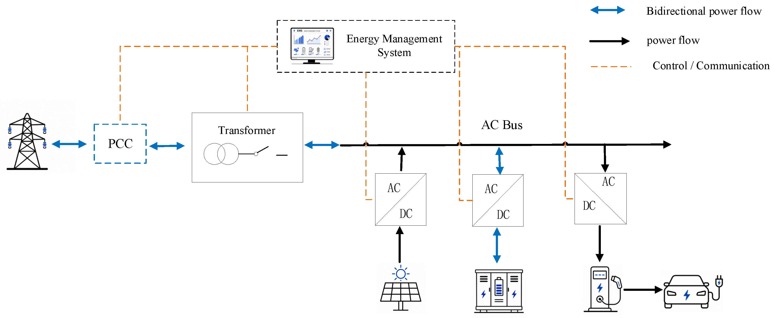
As shown in Figure 1, the photovoltaic–energy storage–charging integrated system investigated in this study for highway service areas adopts an AC-bus-coupled architecture. The system consists of the utility grid, photovoltaic generation units, an energy storage system, DC charging facilities, and an energy management system. Each functional unit is connected to the AC bus through the corresponding power conversion device, while the energy management system is responsible for monitoring the system operating status and coordinating system control.

(1)

Photovoltaic Conversion Module

The photovoltaic conversion module mainly consists of PV arrays, power conditioning equipment such as inverters, grid-connection protection devices, and associated control and protection equipment. Photovoltaic modules are composed of multiple photovoltaic cells connected in series and parallel, and are usually made of silicon materials (such as monocrystalline silicon or polycrystalline silicon). In service areas, photovoltaic modules can be installed on the roofs, open spaces, carports, slopes near service areas, and billboards of the service areas.

(2)

Energy Storage Module

The energy storage module plays an indispensable role in the PV–storage–charging integrated system. The energy storage system can improve the photovoltaic utilization rate of the system. During peak photovoltaic power generation periods (such as noon), surplus electrical energy can be stored in the energy storage system; during periods without photovoltaic power generation such as nights or rainy days, the electrical energy stored in the energy storage system can be dispatched to charge electric vehicles. Meanwhile, the energy storage system can also play the role of peak shaving and valley filling: the system can use stored energy to charge electric vehicles during peak electricity price periods, and purchase electricity from the grid for storage in batteries during off-peak electricity price periods. The energy storage system needs to have characteristics such as high energy density per unit volume, excellent load regulation performance, low system cost, safety, and environmental friendliness.

Currently, energy storage batteries are commonly used as the energy storage components of the system. Common energy storage batteries on the market mainly include lithium ternary batteries, lead–carbon batteries, lithium iron phosphate batteries, lithium titanate batteries, and lead–acid batteries, etc. Each type of battery differs in charging rate, safety, unit cost, and cycle life, and needs to be selected according to the application scenario.

(3)

Grid-Connection and Distribution Module

The grid-connection and distribution module is responsible for realizing power interaction between the on-site power grid and the public power grid. When photovoltaic power generation is excessive, the surplus electrical energy can be fed into the grid through the grid-connection and distribution system to increase system revenue. When photovoltaic power generation is insufficient to meet the electric vehicle charging demand, the power grid can supply electrical energy to the PV–storage–charging system through the grid-connection and distribution system.

(4)

EV Charging Module

The final output terminal of electrical energy in the PV–storage–charging system is the electric vehicle charging pile, which is the ultimate service target of the entire system. Currently, there are four main charging modes for electric vehicle charging stations: slow charging, fast charging, battery swapping, and wireless charging.

The AC slow-charging mode first inputs alternating current (AC) into the on-board charger (OBC) of the EV, and then the OBC converts the AC into direct current (DC) for input into the battery. It has low speed, low power, and long charging time, making it unsuitable for the charging scenario of highway service areas. DC fast-charging piles are equipped with AC-DC converters, which can directly convert AC into DC for input into the EV battery. They have high power and fast charging speed, and can charge the battery to 80% within one hour. Due to the high requirement for charging time of electric vehicles on highways, DC fast-charging piles are the main type of charging piles in highway service areas currently. The battery swapping mode currently accounts for a small proportion of the market, while wireless charging is still in the research stage.

(5)

Dispatch and Control Module

The dispatch and control module is responsible for ensuring the efficient and stable operation of the system. The dispatch and control system performs intelligent dispatch and management by real-time monitoring of photovoltaic power generation output, the state of energy storage batteries, and charging demand. The dispatch and control system can flexibly adjust the system’s operation strategy according to different conditions (such as different weather), thereby improving the utilization rate of photovoltaic electrical energy and increasing system revenue.

2.2. Characteristics of Photovoltaic (PV) Power Generation Units

Photovoltaic (PV) power generation units are an important part of the PV–storage–charging integrated system. Their core function is to convert solar energy into electrical energy using photovoltaic cells, providing clean and renewable energy for the system. The output of photovoltaic power generation depends on various factors. In addition to the performance of photovoltaic modules, factors such as actual solar irradiance and ambient temperature also affect the actual output power of PV systems. Considering the impact of the above factors, the actual PV power generation can be calculated by Equation (1):

$$P_{\mathrm{pv}}=\eta P_{\mathrm{s}}{\displaystyle \frac{A}{A_{\mathrm{st}}}}[1+{\theta }_{\mathrm{T}}(T-T_{\mathrm{ref}})]$$

(1)

Here, $P_{\mathrm{pv}}$ denotes the actual power generated by the PV system, and $P_{\mathrm{s}}$ is the rated power of the PV panel. The symbols $A$ and $A_{\mathrm{st}}$ indicate the actual solar irradiance and the irradiance under standard test conditions, respectively. $T$ represents the actual surface temperature of the PV system, while $T_{\mathrm{ref}}$ refers to the standard reference temperature, generally specified as 25 °C. Furthermore, $\eta$ denotes the efficiency of the PV array, and the power temperature coefficient ${\theta }_{\mathrm{T}}$ is set to $-0.004$ [21].

2.3. Charging and Discharging Characteristics of Energy Storage Systems (ESS)

Battery energy storage technology currently dominates the energy storage market, featuring relatively high efficiency and short response time. In PV–storage–charging integrated charging stations on highways, energy storage devices play a key role, mainly to smooth out the fluctuation and intermittent characteristics of photovoltaic power generation.

The energy stored in the energy storage system at time $t$, denoted by $E(t)$, is determined by its energy level at the preceding time step $E(t-1)$ and the corresponding charging or discharging power. As described in Equation (2), a negative value of $P(t)$ indicates that the system is operating in the charging mode, whereas a positive value represents discharging. The parameters ${\eta }_{\mathrm{c}}$ and ${\eta }_{\mathrm{d}}$ denote the charging and discharging efficiencies of the energy storage system, respectively.

$$\left\{\begin{array}{l}E(t)=E(t-1)-P(t)\Delta t{\eta }_{\mathrm{c}},P(t)<0\hfill \\ E(t)=E(t-1)-{\displaystyle \frac{P(t)\Delta t}{{\eta }_{\mathrm{d}}}},\hspace{1em}P(t)>0\hfill \end{array}\right.$$

(2)

The power and capacity of the energy storage system are also constrained by the upper and lower limits of its rated values:

$$\left\{\begin{array}{l}{P}_{\mathrm{ESS},\min }\le P_{\mathrm{ESS}}\le P_{\mathrm{ESS},\max }\hfill \\ E_{\mathrm{ESS},\min }\le E_{\mathrm{ESS}}\le E_{\mathrm{ESS},\max }\hfill \end{array}\right.$$

(3)

Among them, $P_{\mathrm{ESS}}$ is the rated power of the energy storage system, $P_{\mathrm{ESS},\min }$ and $P_{\mathrm{ESS},\max }$ are its lower and upper limits, respectively; $E_{\mathrm{ESS}}$ is the rated capacity of the energy storage system, and $E_{\mathrm{ESS},\min }$ and $E_{\mathrm{ESS},\max }$ are its lower and upper limits, respectively.

The charging and discharging power constraints of the energy storage system are as follows:

$$\left\{\begin{array}{l}0\le P_{\mathrm{C}}(t)\le P_{\mathrm{C},\max }\hfill \\ 0\le P_{\mathrm{D}}(t)\le P_{\mathrm{D},\max }\hfill \end{array}\right.$$

(4)

Among them, $P_{\mathrm{C}}(t)$ is the charging power of the energy storage system, and $P_{\mathrm{C},\max }$ is its upper limit; $P_{\mathrm{D}}(t)$ is the discharging power of the energy storage system, and $P_{\mathrm{D},\max }$ is its upper limit.

3. Dynamic Calculation of Electric Vehicle Load on Highways Considering Temporal and Spatial Characteristics

During long-distance travel on highways, vehicles enter and exit from service area nodes, and stay at the nodes for charging. Aiming at different traffic volumes and their distinct temporal and spatial distributions, this paper adopts the Monte Carlo algorithm to simulate the actual charging process of vehicles in service areas and calculate the node SOC of each vehicle and the service area load. The specific calculation process is as follows:

(1)

Traffic Flow Allocation

According to the OD matrix information, the initial traffic volume can be allocated to each toll station node, i.e., the number of vehicles that will enter the highway from the toll station in a day. Then, based on the daily traffic flow characteristics, the hourly traffic flow proportion is obtained, thereby calculating the number of vehicles for each “toll station (entry) − toll station (exit)” section per hour.

$$f_0(i)=p_i\cdot N$$

(5)

$$f(h,i)={\displaystyle \frac{f_0(i)\cdot {\mathrm{r}}_{\mathrm{h}}(h)}{\sum {\mathrm{r}}_{\mathrm{h}}}}$$

(6)

$$N_{i,j}(h)={\displaystyle \frac{f(h,i)\cdot {\mathrm{OD}}_{i,j}}{{\displaystyle \sum _k}{\mathrm{OD}}_{i,j}}}$$

(7)

Among them, N is the total daily traffic volume, $f_0(i)$ is the total initial traffic volume at toll station node i within a day, and $p_i$ is the proportion allocated to each toll station from the OD matrix; ${\mathrm{r}}_{\mathrm{h}}(h)$ is the hourly traffic flow proportion within 24 h, and $f(h,i)$ is the initial traffic volume allocated to the toll station each hour; ${\mathrm{OD}}_{i,j}$ is the proportion from toll station node i to toll station node j in the OD matrix, and $N_{i,j}$ is the number of vehicles from service area node i to service area node j per hour.

(2)

Calculation of Vehicle Node SOC

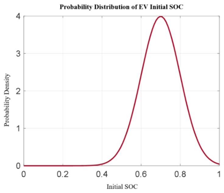
After calculating the number of vehicles in each toll station interval, the charging demand of each vehicle can be calculated. When vehicles enter the highway for long-distance travel, drivers tend to start driving with a high battery level. Therefore, 30% of electric vehicle users are selected to enter the highway with 90% battery charge, and the remaining 70% of vehicles generate the initial SOC based on a normal distribution with parameters (0.7, 0.1) (see Figure 2) [22].

$$S_0=\max (0,\min (\mathcal{N}(0.7,0.1),1))$$

(8)

After assigning an initial SOC to each EV, the arrival SOC at each service area can be calculated. To simulate the impact of factors such as traffic load and weather, a random factor is introduced to represent this fluctuation.

$$S_k=S_0-{\displaystyle \frac{\Delta d\cdot E_{\mathrm{avr}}}{P_{\mathrm{bat}}}}\cdot \xi$$

(9)

Among them, $S_k$ is the state of charge (SOC) when the vehicle arrives at service area i, $S_0$ is the initial SOC when the vehicle enters the highway, $\Delta d$ is the driving distance, $E_{\mathrm{avr}}$ is the energy consumption per kilometer of the EV, and $P_{\mathrm{bat}}$ is the EV battery capacity. $\xi$ is a random variable following a normal distribution N(1, 0.1), and the energy consumption can fluctuate within the range of ±10% of the reference value.

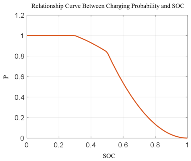
The charging probability varies with the value of arrival SOC, as shown in Figure 3 [23].

$$P=\left\{\begin{array}{c}1,SOC\le 0.3\\ -SO{C}^2+1.09,0.3<SOC\le 0.5\\ 3.36{(SOC-1)}^2,0.5<SOC\le 1\end{array}\right.$$

(10)

Accordingly, when the i-th EV passes through service area node k, its SOC can be updated as follows:

$$S_i=S_0-{\displaystyle \frac{\Delta d\cdot E_{\mathrm{avr}}}{P_{\mathrm{bat}}}}+{\displaystyle \sum _{k=1}^N}{y}_k{z}_{i,k}(S_{\mathrm{up}}-S_{i,k})$$

(11)

Among them, N is the number of the passed location node; $y_k$ is a node discrimination function. If the node is a service area node, $y_k=1$, otherwise $y_k=0$. $z_{i,k}$ is a charging selection function, used to determine whether the i-th EV chooses to charge when passing through the k-th node. If it charges, $z_{i,k}=1$, otherwise $z_{i,k}=0$; $S_{\mathrm{up}}$ is the SOC value when the EV is fully charged; $S_{i,k}$ is the SOC value of the i-th EV when passing through the node numbered k [4].

(3)

EV Charging Time

The arrival SOC of the electric vehicle is calculated from Equation (11), and its charging time can be calculated as follows:

$$T_{\mathrm{c}}={\displaystyle \frac{\left(1-S_k\right)E_{\mathrm{bat}}}{\eta P_{\mathrm{c}}}}$$

(12)

where $T_{\mathrm{c}}$ denotes the time required to charge the EV, $S_k$ represents the vehicle’s state of charge upon arrival, and $E_{\mathrm{bat}}$ is the energy capacity of the EV battery. In addition, $\eta$ and $P_{\mathrm{c}}$ refer to the charging efficiency and charging power of the charging pile, respectively.

(4)

Charging Load Allocation

Within each hourly time interval, the charging time of the EV may exceed 1 h. If $T_{\mathrm{c}}$ is less than or equal to 1 h, charging can be completed within the current time interval. If it exceeds 1 h, the charging load needs to be allocated to subsequent time intervals.

$$P_{\mathrm{EV}}\left(h\right)=\eta P_{\mathrm{c}}\cdot \min (T_{\mathrm{c}},1)$$

(13)

According to the required charging time, the charging load is allocated among multiple hours. If $T_{\mathrm{c}}$ is greater than 1, in the next hour, the charging load of the EV is as follows:

$$P_{\mathrm{EV}}(h+1)=\eta P_{\mathrm{c}}\cdot \min (T_{\mathrm{c}}-1,1)$$

(14)

(5)

Calculating the Average Value by Monte Carlo Method

After performing multiple simulations of the above process, the average charging power of electric vehicles in highway service areas can be calculated by finding the average value using the Monte Carlo method.

$$P_{\mathrm{EV}}(h,n)\approx {\displaystyle \frac{1}{M}}{\displaystyle \sum _{i=1}^M{P}_{\mathrm{EV}}(h,n)}$$

(15)

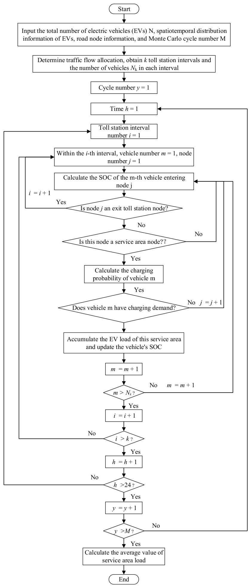
In summary, the load forecasting process of electric vehicles in highway service areas based on the Monte Carlo method is shown in Figure 4:

4. Calculation of Electric Vehicle Waiting Time Based on Queuing Theory

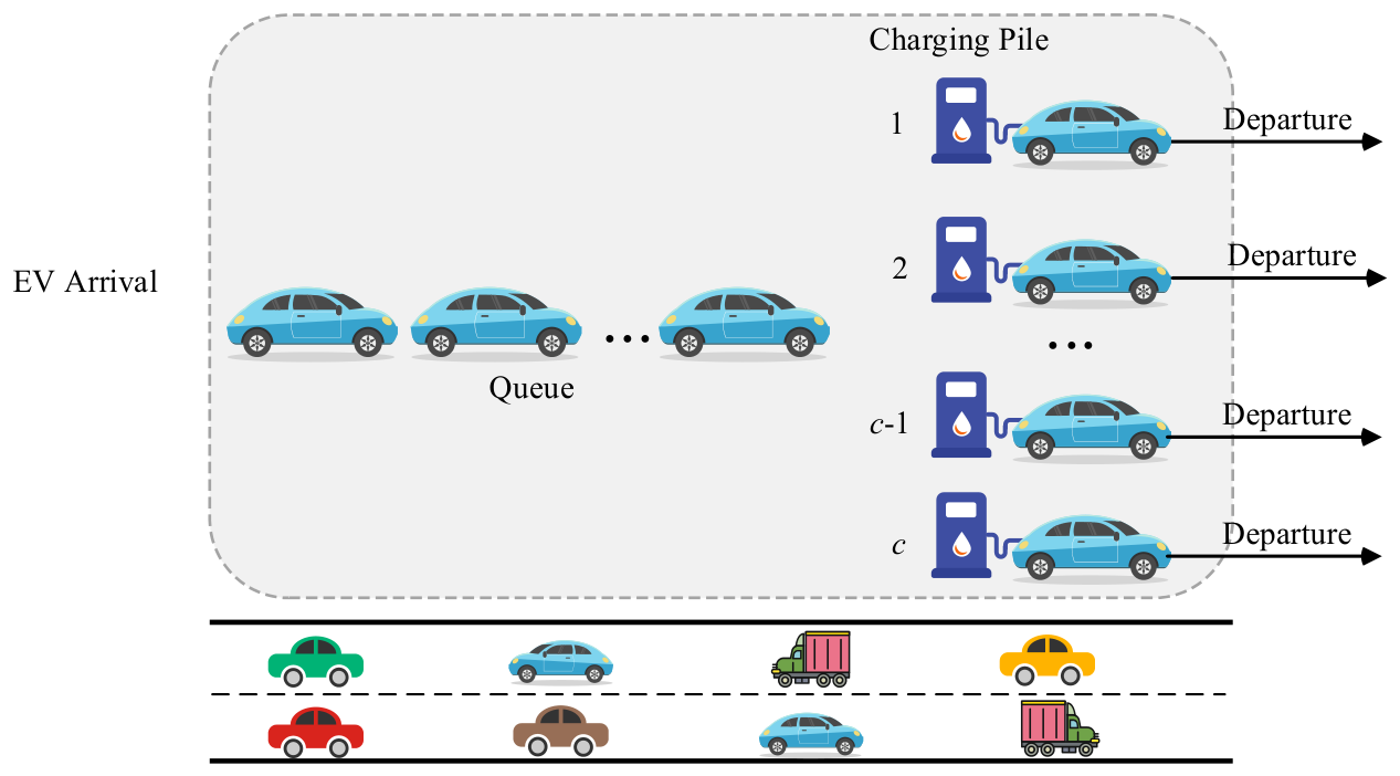
The queuing process of electric vehicles at PV–storage–charging integrated charging stations in highway service areas is shown in Figure 5. The M/M/c multi-server queuing model is adopted to calculate the vehicle waiting time, where the system consists of $c$ independently operated service servers, i.e., $c$ charging piles. Within each hourly interval, the EV arrival process is approximated as a homogeneous Poisson process with the corresponding arrival rate, while the charging service time is assumed to follow an exponential distribution. Vehicles are served according to the First Come First Served (FCFS) principle. When an EV arrives at the service area, the system assigns an available charging pile according to the current operating status. If all charging piles are occupied, the newly arriving EV joins the waiting queue and leaves the system after charging is completed [24].

The M/M/c model is mainly adopted in this study to estimate the vehicle waiting time under different charging-facility configurations and to incorporate it into the subsequent capacity optimization. The Monte Carlo simulation has already considered the randomness of EV arrival SOC and charging demand, while the average service rate in the queuing model is determined according to the average charging energy demand, charging-pile power, and charging efficiency. Since this study focuses on the overall average queuing performance of service areas under different capacity configurations rather than the detailed charging-time distribution of individual EVs, the M/M/c model is considered sufficient for the purpose of this study. However, the actual charging time of EVs may also be affected by arrival SOC, vehicle parameters, and charging behavior, and its distribution may therefore be more complex than an exponential distribution. The M/G/c model can account for a more general service-time distribution, but it also increases the complexity of waiting-time calculation and the subsequent optimization process. Therefore, the M/M/c model is retained in this study for capacity-planning analysis.

In this queuing model, n is the number of arriving vehicles, μ is the average service rate of one service desk, then the average service rate of c homogeneous service desks is cμ (when n ≥ c) or nμ (when n < c). The service intensity $\rho =\lambda /(c\mu )$ reflects the average utilization level of the service facility [24]. Figure 6 shows the state transition process of the M/M/c multi-server queuing system.

The calculation process of the average queuing time based on the above parameters is as follows:

(1)

EV Arrival Rate

Highway traffic flow exhibits pronounced time-of-day variations; therefore, this study does not assume a constant EV arrival rate over the entire day. Based on the hourly traffic flow and charging demand at each service area obtained from the Monte Carlo simulation described in Section 3, the average EV arrival rate at service area $i$ during time interval $t$, denoted by ${\lambda }_{i,t}$, can be determined. Since a 1 h interval is adopted as the basic time resolution for traffic-flow and charging-load calculations, the arrival rate is assumed to remain approximately constant within each hourly interval. Accordingly, the EV arrival process within each interval is approximated as a homogeneous Poisson process with arrival rate ${\lambda }_{i,t}$. Over the entire day, the EV arrival process can therefore be regarded as a time-varying Poisson process with a piecewise-constant arrival rate. This local stationary approximation has been widely adopted in the analysis of time-varying multi-server queueing systems and EV charging systems [25,26,27]. Under this assumption, the time interval between two successive EV arrivals within each hourly interval follows an exponential distribution, which can be expressed as follows:

$$f_{\mathrm{T}}(\Delta t)={\lambda }_{i,t}{\mathrm{e}}^{-{\lambda }_{i,t}\Delta t}\hspace{1em}\Delta t>0$$

(16)

$${\lambda }_{i,t}=q(x_i,t)$$

(17)

where ${\lambda }_{i,t}$ denotes the average EV arrival rate at service area $i$ during hourly interval $t$, and $q\left(x_i,t\right)$ represents the corresponding EV traffic flow obtained from the Monte Carlo-based load calculation process shown in Figure 4. $\Delta t$ denotes the inter-arrival time between two successive EVs within the considered hourly interval, and $f_T\left(\Delta t\right)$ is its probability density function. It should be noted that ${\lambda }_{i,t}$ is assumed to be approximately constant only within each individual hourly interval, while its value is allowed to vary across different service areas and different time intervals.

(2)

Service Rate of Charging Pile System in Service Areas

Parameter μ is the average service rate, referring to the number of vehicles that a single charging pile can serve per hour, and its calculation method is shown in Equation (18):

$$\mu ={\displaystyle \frac{P_{\mathrm{c}}\times \eta }{E_{\mathrm{ave}\text{\_}i}}}$$

(18)

Among them, $P_{\mathrm{c}}$ is the power of the charging pile, $\eta$ is the charging efficiency, and $E_{\mathrm{ave}\text{\_}i}$ is the average charging energy demand of the service area.

(3)

Service Intensity of Charging Pile System in Service Areas

Based on the above parameters, the service intensity ρ of the queuing system can be obtained from Equation (19).

$$\rho ={\displaystyle \frac{\lambda }{c\times \mu }}$$

(19)

When the service intensity $\rho <1$, that is, the number of customers arriving per unit time is lower than the processing capacity of the service desks, the queuing system can enter a stable operation state. Based on statistical knowledge, the following indicators can be calculated:

The probability $P_0$ that no customers arrive in a time period, and the probability $P_n$ that n customers arrive:

$$\left\{\begin{array}{c}{P}_0={\left[{\displaystyle \sum _{k=0}^{c-1}}{\displaystyle \frac{1}{k!}}{({\displaystyle \frac{\lambda }{\mu }})}^k+{\displaystyle \frac{1}{c!}}{\displaystyle \frac{1}{1-\rho }}{({\displaystyle \frac{\lambda }{\mu }})}^c\right]}^{-1}\\ P_n=\left\{\begin{array}{cc}{\displaystyle \frac{1}{n!}}{({\displaystyle \frac{\lambda }{\mu }})}^n{P}_0& n\le c\\ {\displaystyle \frac{1}{c!c^{n-c}}}{({\displaystyle \frac{\lambda }{\mu }})}^n{P}_0& n>c\end{array}\right.\end{array}\right.$$

(20)

The average queue length $L_q$ is:

$$L_{\mathrm{q}}={\displaystyle \frac{{(c\rho )}^c\rho }{c!{(1-\rho )}^2}}{P}_0$$

(21)

Among them, $c\rho ={\displaystyle \frac{\lambda }{\mu }},k=n-c$.

The average system length $L_s$ is as follows:

$$L_{\mathrm{s}}=L_{\mathrm{q}}+{\displaystyle \frac{\lambda }{\mu }}={\displaystyle \frac{{(c\rho )}^c\rho }{c!{\left(1-\rho \right)}^2}}{P}_0+{\displaystyle \frac{\lambda }{\mu }}$$

(22)

The average waiting time $W_{\mathrm{q}}$ of customers is as follows:

$$W_{\mathrm{q}}={\displaystyle \frac{L_{\mathrm{q}}}{\lambda }}={\displaystyle \frac{{\left(c\rho \right)}^c\rho }{c!{\left(1-\rho \right)}^2\lambda }}{P}_0$$

(23)

The average residence time $W_{\mathrm{s}}$ of customers is as follows:

$$W_{\mathrm{s}}={\displaystyle \frac{L_{\mathrm{s}}}{\lambda }}={\displaystyle \frac{{\left(c\rho \right)}^c\rho }{c!{\left(1-\rho \right)}^2\lambda }}{P}_0+{\displaystyle \frac{1}{\mu }}$$

(24)

5. Capacity Configuration and Solution Model of PV–Storage–Charging System in Service Areas

5.1. Optimization Objectives

The optimization objectives include the construction and maintenance costs of the highway PV–storage–charging system, as well as the comprehensive waiting time for vehicle owners, which comprehensively considers the average waiting time, worst-case waiting time, and the carrying capacity of charging piles.

a.

Construction and Maintenance Costs

$$f_1(x)=C_{\mathrm{cstr}}^{\mathrm{sta}}+C_{\mathrm{cstr}}^{\mathrm{stor}}+C_{\mathrm{cstr}}^{\mathrm{pv}}+C_{\mathrm{mitn}}^{\mathrm{sta}}+C_{\mathrm{mitn}}^{\mathrm{stor}}+C_{\mathrm{mitn}}^{\mathrm{pv}}$$

(25)

The calculation of construction costs is shown in Equation (26) [4]:

$$\begin{array}{l}{C}_{\mathrm{cstr}}^{\mathrm{sta}}={\displaystyle \frac{r_0{\left(1+r_0\right)}^z}{{\left(1+r_0\right)}^z-1}}{\displaystyle \sum _{i=1}^N}\left(c_{\mathrm{a}}+N_i^{\mathrm{ap}}{C}_{\mathrm{ap}}\right)\\ C_{\mathrm{cstr}}^{\mathrm{stor}}={\displaystyle \frac{r_1{\left(1+r_1\right)}^z}{{\left(1+r_1\right)}^z-1}}{\displaystyle \sum _{i=1}^N}\left(c_{\mathrm{b}}+N_i^{\mathrm{bp}}{C}_{\mathrm{bp}}\right)\\ C_{\mathrm{cstr}}^{\mathrm{pv}}={\displaystyle \frac{r_2{\left(1+r_2\right)}^z}{{\left(1+r_2\right)}^z-1}}{\displaystyle \sum _{i=1}^N}\left(c_{\mathrm{c}}+N_i^{\mathrm{cp}}{C}_{\mathrm{cp}}\right)\end{array}$$

(26)

Among them, N represents the total number of system nodes; $c_{\mathrm{a}}$, $c_{\mathrm{b}}$, $c_{\mathrm{c}}$ represent the fixed installation costs of charging piles, energy storage, and photovoltaic equipment; $N_i^{\mathrm{ap}}$, $N_i^{\mathrm{cp}}$ are the number of charging stations and photovoltaic units at node i; $N_i^{\mathrm{bp}}$ represents the energy storage capacity at node i; $C_{\mathrm{ap}}$, $C_{\mathrm{cp}}$ are the unit costs of charging piles and photovoltaic equipment, respectively; $C_{\mathrm{bp}}$ is the unit capacity cost of the energy storage system; $r_0$, $r_1$, $r_2$ are the discount rates for charging piles, energy storage, and photovoltaics; z is the project operation period.

The maintenance cost also consists of the maintenance costs of charging piles, energy storage, and photovoltaics, and there is a certain proportional relationship with the construction cost. The calculation of maintenance cost is shown in Equation (27) [28]:

$$\begin{array}{l}{C}_{\mathrm{mitn}}^{\mathrm{sta}}=\delta {\displaystyle \frac{r_0{\left(1+r_0\right)}^z}{{\left(1+r_0\right)}^z-1}}{\displaystyle \sum _{i=1}^N}\left(c_{\mathrm{a}}+N_i^{\mathrm{ap}}{C}_{\mathrm{ap}}\right)\\ C_{\mathrm{mitn}}^{\mathrm{stor}}=\delta {\displaystyle \frac{r_1{\left(1+r_1\right)}^z}{{\left(1+r_1\right)}^z-1}}{\displaystyle \sum _{i=1}^N}\left(c_{\mathrm{b}}+N_i^{\mathrm{bp}}{C}_{\mathrm{bp}}\right)\\ C_{\mathrm{mitn}}^{\mathrm{pv}}=\delta {\displaystyle \frac{r_2{\left(1+r_2\right)}^z}{{\left(1+r_2\right)}^z-1}}{\displaystyle \sum _{i=1}^N}\left(c_{\mathrm{c}}+N_i^{\mathrm{cp}}{C}_{\mathrm{cp}}\right)\end{array}$$

(27)

Among them, $\delta$ is the conversion coefficient, taking 0.04.

b.

Comprehensive Waiting Time Cost of Vehicle Owners under Multidimensions

To improve the charging quality of service areas, when configuring the capacity of PV–storage–charging systems, in addition to optimizing the total queuing time of vehicle owners, the queuing situation of the worst-performing service area and the carrying capacity of charging pile configuration for traffic flow should also be considered. Therefore, this paper proposes the comprehensive waiting time cost of vehicle owners under multidimensions, which comprehensively considers the weighted average waiting time, the waiting time of the worst service area, and the penalty when the number of charging piles has difficulty supporting the current traffic flow. The objective function $f_2(x)$ related to the queuing time of vehicle owners is shown in Equation (28):

$$f_2(x)=\mathrm{a}\cdot W_{\mathrm{q}}^{\mathrm{avr}}+b\cdot W_{\mathrm{q}}^{\max }+c\cdot P$$

(28)

Among them, a, b and c are the weight coefficients of $W_{\mathrm{q}}^{\mathrm{avr}}$, $W_{\mathrm{q}}^{\max }$, and P, taking 0.4, 0.3, and 0.3 respectively. Since the weighted average waiting time reflects the overall service level of the system, it is assigned a slightly higher weight. The maximum waiting time and the overload penalty reflect local congestion and system operating pressure, respectively, and are therefore assigned equal weights. This weighting scheme is intended to balance the overall service level, local congestion, and high-load operation of the system. $\gamma$ is the conversion coefficient of the influence of flow intensity on waiting time, taking 500.

The average queuing time of each service area in each time period can be calculated from Equation (23), and accordingly, the weighted average waiting time of all service areas can be calculated:

$$W_{\mathrm{q}}^{\mathrm{avr}}={\displaystyle \frac{{\displaystyle \sum _{i=1}^M}{\displaystyle \sum _{h=1}^{24}}\lambda (h,i)\cdot W_{\mathrm{q}}(h,i)}{{\displaystyle \sum _{i=1}^M}{\lambda }_i}}$$

(29)

where $W_{\mathrm{q}}^{\mathrm{avr}}$ denotes the weighted mean waiting time across all service areas, and $M$ represents the total number of service areas. The index $h$ refers to the hourly time interval. $\lambda (h,i)$ is the number of vehicles arriving at the $i$-th service area during the $h$-th interval, while $W_{\mathrm{q}}(h,i)$ denotes the corresponding average queueing time. In addition, ${\lambda }_i$ represents the total number of vehicles arriving at the $i$-th service area over the entire day.

The waiting time of the worst-performing service area usually reflects the most congested situation in the system and may have a significant impact on the overall user experience. Its calculation is shown in Equation (30):

$$W_{\mathrm{q}}^{\max }=\max (W_{\mathrm{q}}(h,i))$$

(30)

In order to avoid the situation where the charging pile configuration cannot meet the current vehicles and causes the queuing system to collapse when the traffic flow is too large, the service intensity ρ of the system should be constrained. Therefore, a penalty is imposed on the situation where ρ is large in the objective function to ensure that resource allocation can be dynamically adjusted according to the current state during the optimization process. The penalty function when ρ > 0.90 is shown in Equation (31):

$$P=\gamma {\displaystyle \sum _{i=1}^M}{\displaystyle \sum _{h=1}^{24}}\max {(0,\rho (h,i)-0.9)}^2$$

(31)

5.2. Constraints

a.

Upper and Lower Bound Constraints of Variables

$$\left\{\begin{array}{c}{N}_{\mathrm{pv},\min }\le {N_{\mathrm{pv}}}^i\le N_{\mathrm{pv},\max }\\ P_{\mathrm{ess},\min }\le {P_{\mathrm{ESS}}}^i\le P_{\mathrm{ess},\max }\\ N_{\mathrm{ch},\min }\le {N_{\mathrm{ch}}}^i\le N_{\mathrm{ch},\max }\end{array}\right.$$

(32)

For the $i$-th service area, ${N_{\mathrm{pv}}}^i$ denotes the installed number of PV modules, which is restricted by the lower and upper limits $N_{\mathrm{pv},\min }$ and $N_{\mathrm{pv},\max }$, respectively. Similarly, ${P_{\mathrm{ESS}}}^i$ represents the power of the energy storage system, with $P_{\mathrm{ess},\min }$ and $P_{\mathrm{ess},\max }$ specifying its allowable range. The variable ${N_{\mathrm{ch}}}^i$ indicates the number of charging piles, whose minimum and maximum values are given by $N_{\mathrm{ch},\min }$ and $N_{\mathrm{ch},\max }$, respectively.

b.

Module Quantity Constraints

In highway service areas, due to limited space, the total number of charging piles and photovoltaic power generation modules must also be subject to certain restrictions to ensure the rational use of the site. Since energy storage modules occupy less space, no strict space restrictions are set during configuration, and they can be flexibly arranged according to needs.

$$N_{\mathrm{ch}}^i+N_{\mathrm{pv}}^i\le N_{\max }^i$$

(33)

Among them, $N_{\mathrm{ch}}^i$ and $N_{\mathrm{pv}}^i$ are the number of charging piles and photovoltaic modules at the i-th service area node, respectively, and $N_{\max }^i$ represents the maximum total number of these two types of modules.

c.

Queuing Time Constraint

When vehicle owners enter the service area to receive charging, they are usually unwilling to wait for a long time. Therefore, the queuing time needs to be set with reasonable limits to ensure efficient charging services and enhance user experience.

$$W_{\mathrm{q}}<W_{\mathrm{limit}}$$

(34)

Among them, $W_{\mathrm{limit}}$ represents the maximum customer tolerance time.

d.

Power Balance Constraint

To ensure the reliable power supply of the microgrid in the highway service area, the power supply capacity needs to be greater than or equal to the maximum demand of the charging load, so as to ensure that the system can meet the charging demand at any time and avoid resource waste or insufficient power supply caused by insufficient or excessive equipment.

$$P_{\mathrm{pv}\text{\_}\max }+P_{\mathrm{ess}\text{\_}\max }+P_{\mathrm{grid}\text{\_}\max }\ge P_{\mathrm{load},\max }$$

(35)

Here, $P_{\mathrm{pv}\text{\_}\max }$, $P_{\mathrm{ess}\text{\_}\max }$, and $P_{\mathrm{grid}\text{\_}\max }$ represent the maximum PV generation power, the maximum discharge power of the energy storage system, and the maximum power exchanged through the grid tie-line, respectively. $P_{\mathrm{load},\max }$ denotes the forecast maximum load demand.

e.

Photovoltaic Power Generation Proportion Constraint

To reduce dependence on the power grid and make full use of renewable energy for power supply, the minimum configuration of photovoltaic power generation is required to support a certain proportion of electrical load.

$${\displaystyle \frac{P_{\mathrm{pv}}}{P_{\mathrm{load}}}}\ge R$$

(36)

Among them, R is the minimum photovoltaic power supply proportion.

f.

Grid Peak Regulation Constraint

To improve the system’s self-sufficiency capability and reduce the impact of peak load on the power grid, the peak load is required to be provided by a certain proportion of photovoltaic and energy storage.

$${\displaystyle \frac{P_{\mathrm{pv}\text{\_}\max }+P_{\mathrm{ess}\text{\_}\max }}{P_{\mathrm{load},\max }}}\ge H$$

(37)

Among them, H is the minimum power supply proportion of photovoltaic and energy storage at load peak.

5.3. Model Solution

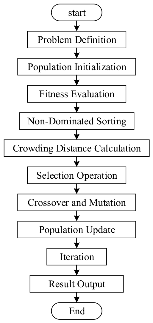
To balance multiple solution objectives, this paper adopts the genetic algorithm for multi-objective optimization solution. The specific steps of the solution are shown in Figure 7.

When using intelligent optimization methods such as genetic algorithms to solve multi-objective problems, the obtained Pareto front is actually a set composed of numerous non-dominated solutions. Due to the trade-off relationship between various optimization objectives, improving the performance of one objective may often lead to a decrease in the performance of other objectives. Therefore, after obtaining the Pareto optimal solution set, further decision-making is required if a unique solution is to be obtained. This study will adopt the VIKOR method to accomplish this decision-making process.

Consider a set of J feasible solutions $a_1,a_2,\dots ,a_J$, where $f_{ij}$ is the i-th objective function value of $a_J$, and n is the number of objective functions to be optimized.

$$L_{p,j}={\left\{{\displaystyle \sum _{i=1}^n}{\left[w_i\left(f_i^{\ast }-f_{ij}\right)/\left(f_i^{\ast }-f_i^{-}\right)\right]}^p\right\}}^{1/p}$$

(38)

Among them, $1\le p\le \infty ;j=1,2,\dots ,J$.

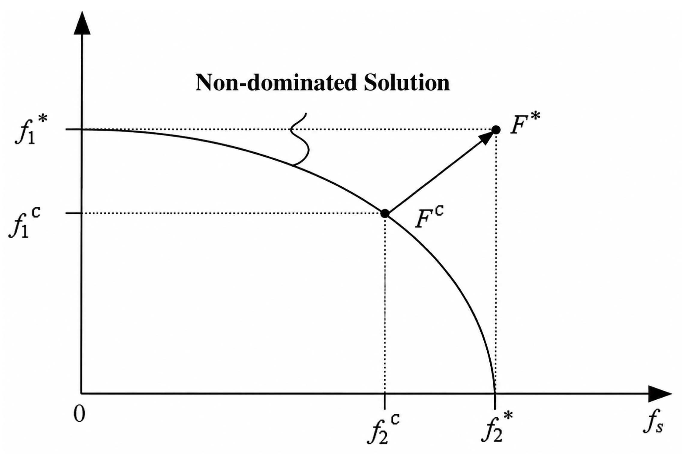
The VIKOR method uses $S_j$ and $R_j$, which correspond to the $L_{1,j}$ and $L_{\infty ,j}$ metrics, respectively, as the ranking criteria. Minimizing $S_j$ maximizes group utility, whereas minimizing $R_j$ minimizes individual regret. Among them, the solution based on ${\min }_j{S}_j$ can maximize group utility, while the solution based on ${\min }_j{R}_j$ can minimize individual regret. As shown in Figure 8, the compromise solution $F^C$ is closest to the ideal solution $F^{*}$, reflecting the mutual compromise among various criteria. Considering the bi-objective optimization scenario, after compromise processing, the deviation between each optimization objective and its ideal value can be expressed as $\Delta f_1=f_1^{\ast }-f_1^c$ and $\Delta f_2=f_2^{\ast }-f_2^c$.

The decision-making ranking process of the VIKOR method includes the following key steps:

a.

The decision-maker assigns weight values to each evaluation criterion

$$\beta ={\left[\begin{array}{c}{\beta }_1,{\beta }_2,\dots ,{\beta }_n\end{array}\right]}^T$$

(39)

Among them, ${\beta }_i$ represents the relative weight coefficient of the i-th criterion.

b.

For each evaluation criterion, the ideal solution and the nadir solution need to be calculated separately. When the i-th objective function is of the benefit type,

$$f_i^{\ast }=\underset{j}{\max }{f}_{ij},f_i^{-}=\underset{j}{\min }{f}_{ij}$$

(40)

If it is a cost-type criterion, then

$$f_i^{\ast }=\underset{j}{\min }{f}_{ij},f_i^{-}=\underset{j}{\max }{f}_{ij}$$

(41)

Among them, $i=1,2,\dots ,n$.

c.

Calculate $S_j$ and $R_j$, $j=1,2,\dots ,J$:

$$\begin{array}{c}{S}_j={\displaystyle \sum _{i=1}^n}{\beta }_i\left(f_i^{\ast }-f_{ij}\right)/\left(f_i^{\ast }-f_i^{-}\right)\\ R_j=\underset{i}{\max }\left[{\beta }_i\left(f_i^{\ast }-f_{ij}\right)/\left(f_i^{\ast }-f_i^{-}\right)\right]\end{array}$$

(42)

d.

Calculate $Q_j$, $j=1,2,\dots ,J$:

$$Q_j=v\left(S_j-S^{\ast }\right)/\left(S^{-}-S^{\ast }\right)+\left(1-v\right)\left(R_j-R^{\ast }\right)/\left(R^{-}-R^{\ast }\right)$$

(43)

Among them, $S^{*}={\min }_j{S}_j$, $S^{-}={\max }_j{S}_j$, $R^{\ast }={\min }_j{R}_j$, $R^{-}={\max }_j{R}_j$. Here, v represents the weight coefficient of group utility (usually set to 0.5), and 1-v corresponds to the weight value of individual regret.

e.

After sorting the candidate solutions in ascending order of $Q_j$ values, let $A_1$ and $A_2$ be the top two ranked alternatives. To determine $A_1$ as the optimal compromise solution, the following two conditions need to be satisfied:

(1)

$Q(A_2)-Q(A_1)\ge 1/\left(J-1\right)$;

(2)

$A_1$ is also ranked first according to at least one of the S and R rankings.

When condition (2) is not satisfied, both $A_1$ and $A_2$ are proposed as compromise solutions.

If condition (1) is not satisfied, a set of compromise solutions is formed, including $A_1,A_2,\dots ,A_m$, where A_m is the alternative with the largest rank index satisfying

Q(A_m) − Q(A₁) < 1/(J − 1).

All alternatives in this set are reported as compromise solutions.

6. Case Study

6.1. Case Parameters

To simplify the calculations, this study assumes that all electric vehicles have identical battery parameters. The specific parameters of the electric vehicles and the highway route are provided in

Table 1. Basic parameters of electric vehicles and the highway route.

Parameter	Value
Battery capacity	55 kW·h
Energy consumption per kilometer	0.15 kW·h/km
Charging pile power	80 kW
Charging efficiency	90%
Total length of the highway route	640 km
Distance between adjacent nodes	40 km

. Following Ref. [4], the EV battery capacity, energy consumption per kilometer, and distance between adjacent nodes are set to 55 kWh, 0.15 kWh/km, and 40 km, respectively. To compare the differences in the capacity configuration schemes of the photovoltaic–energy storage–charging system at highway service areas under different daily electric vehicle traffic volumes, two scenarios with daily electric vehicle traffic volumes of 4000 and 6000 vehicles are analyzed.

The OD distribution and temporal traffic-flow profile used in this case study are adopted from the historical-data-based case study reported in Ref. [4], as shown in

Table 2. Distribution of electric vehicle trips across OD pairs.

Origin Node	Destination Node	Proportion of Trips
Node a	Node e	13%
Node a	Node i	7%
Node a	Node m	5%
Node a	Node q	2%
Node e	Node i	22%
Node e	Node m	8%
Node e	Node q	4%
Node i	Node m	18%
Node i	Node q	9%
Node m	Node q	12%

.

Parameters related to the construction of the PV–energy storage–charging system are shown in

Table 3. PV–storage–charging construction parameters of highway service areas.

Parameter	Value	Parameter	Value
Fixed Cost of PV Modules	40,000 yuan	Operation Life	25
Fixed Cost of Energy Storage System	800,000 yuan/MW·h	Capacity of a Single PV Module	30 kW
Fixed Cost of a Single Charging Pile	60,000 yuan	Discount Rate of PV	0.08
Discount Rate of Energy Storage	0.07	Maintenance Cost Conversion Coefficient	0.04
Upper/Lower Limit of PV Module Quantity	35/10	Upper/Lower Limit of Energy Storage Capacity	6000/ 1000 kW·h
Upper/Lower Limit of Charging Pile Quantity	25/5	Maximum Continuous Energy Storage Duration	2 h
Total Number of Vehicles Under Conventional Load	4000 vehicles	Maximum Queuing Duration Under Conventional Load	15 min
Total Number of Vehicles Under High-Load Scenario	6000 vehicles	Maximum Queuing Duration Under High Load	20 min
Maximum Grid Access Power	1000 kW

[4]. When the VIKOR method is used to rank the obtained Pareto-optimal solutions, the criterion-weight vector is set to $\beta ={\left[\begin{array}{c}0.7,0.3\end{array}\right]}^T$, where the first weight corresponds to the construction and maintenance cost and the second corresponds to the comprehensive waiting-time cost. Considering that user waiting time has already been constrained in the optimization model, a higher weight is assigned to the construction and maintenance cost in the VIKOR ranking stage to further balance the economic performance of the solution while satisfying the service-level requirements. The group-utility coefficient is set to v = 0.5.

The main parameter settings of the genetic algorithm are shown in

Table 4. Main parameters of the multi-objective genetic algorithm.

Parameter	Value
Population size	300
Maximum number of generations	400
Convergence tolerance	${5\times 10}^{-5}$
Crossover probability	0.85
Mutation probability	0.15

.

6.2. Analysis of Simulation Results

To investigate the configuration characteristics of highway service-area photovoltaic–energy storage–charging systems under different traffic demand levels, two scenarios are considered: a normal-load scenario and a high-load scenario. In the normal-load scenario, the total number of electric vehicles traveling on the highway over a full day is set to 4000 to represent typical daily traffic conditions. In the high-load scenario, the daily number of electric vehicles is set to 6000 to represent surges in travel demand during holidays or increases in electric vehicle penetration in the future. These two scenarios represent only typical demand levels, and the model’s robustness under more diverse traffic conditions remains to be further examined.

Table 5. Optimal configuration results of the PV–energy storage–charging system at each service area under two load scenarios.

Service Area ID	Load Scenario	Number of PV Modules	Energy Storage System Capacity (kWh)	Number of Charging Piles
a	Normal Load	12	2654	5
	High Load	16	1824	5
b	Normal Load	13	1026	6
	High Load	29	2946	7
c	Normal Load	10	1620	9
	High Load	17	2956	13
d	Normal Load	11	1792	10
	High Load	25	3352	14
e	Normal Load	16	1294	7
	High Load	23	2712	11
f	Normal Load	17	1554	13
	High Load	30	3348	20
j	Normal Load	15	1030	14
	High Load	25	1154	16
h	Normal Load	19	2812	10
	High Load	32	2516	14
i	Normal Load	11	2096	11
	High Load	31	2732	17
g	Normal Load	15	3006	8
	High Load	26	3496	12
k	Normal Load	12	2346	10
	High Load	25	3038	10
l	Normal Load	14	1374	12
	High Load	29	3442	10

presents the optimal capacities of photovoltaic modules, energy storage systems, and charging piles at each service area under the two load scenarios.

The simulation and optimization results for the two scenarios are analyzed separately below.

(1)

Normal-load scenario

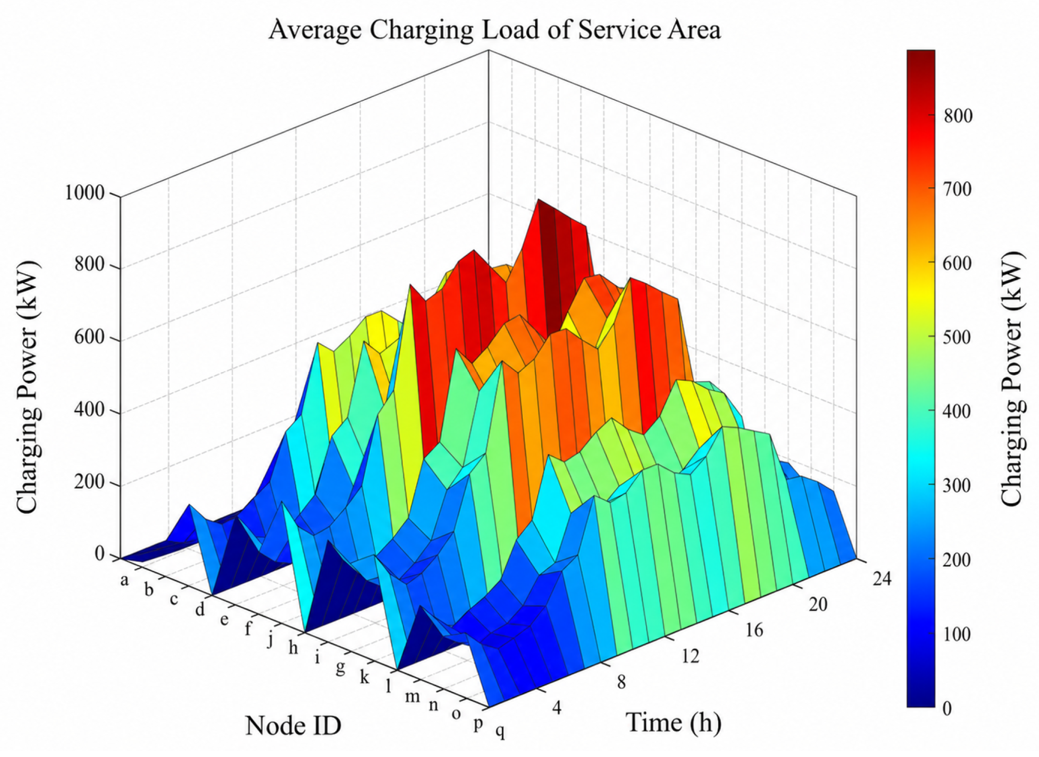
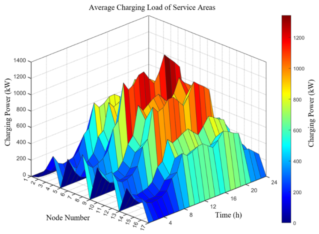
Based on the spatiotemporal distribution characteristics of electric vehicles, the charging loads at the service areas are predicted through simulation, as shown in Figure 9.

From the temporal perspective, the period from 9:00 to 20:00 constitutes the peak-load period, which is consistent with the temporal distribution of traffic flow. In contrast, the predicted charging load decreases significantly at night, indicating that the load forecasting model can accurately capture the characteristics of actual traffic flow. From the spatial perspective, service-area nodes $f$–$h$ and j–$l$ experience relatively high traffic volumes. Significant differences in charging load are observed among the nodes, and the spatial distribution of the load is highly correlated with the OD flow matrix, demonstrating the direct influence of traffic flow on charging demand.

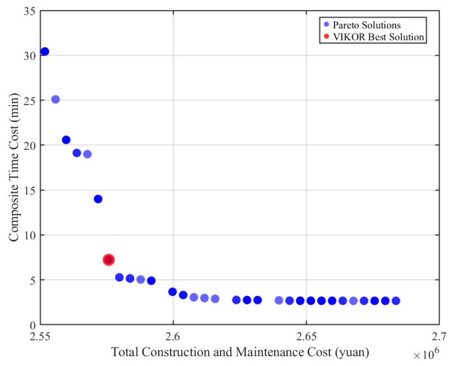
Figure 10 presents the Pareto front for the normal-load scenario, which can be divided into three characteristic regions. The upper-left region corresponds to high waiting times, where construction and maintenance costs are relatively low but the service quality is poor because insufficient equipment capacity results in excessive service pressure. The lower-right region is relatively flat, with the comprehensive waiting time remaining below 5 min. In this region, further investment produces only limited improvements in service quality, indicating diminishing marginal benefits. The middle region exhibits a rapid decline and therefore represents the range in which additional investment yields the most significant benefits.

The red dot in Figure 10 denotes the optimal solution selected from all non-dominated solutions under the specified weighting coefficient. Under this solution, the total construction and maintenance cost is RMB 2.5758 million, and the comprehensive time cost for EV users is 7.23 min, achieving an optimal trade-off between cost and service quality.

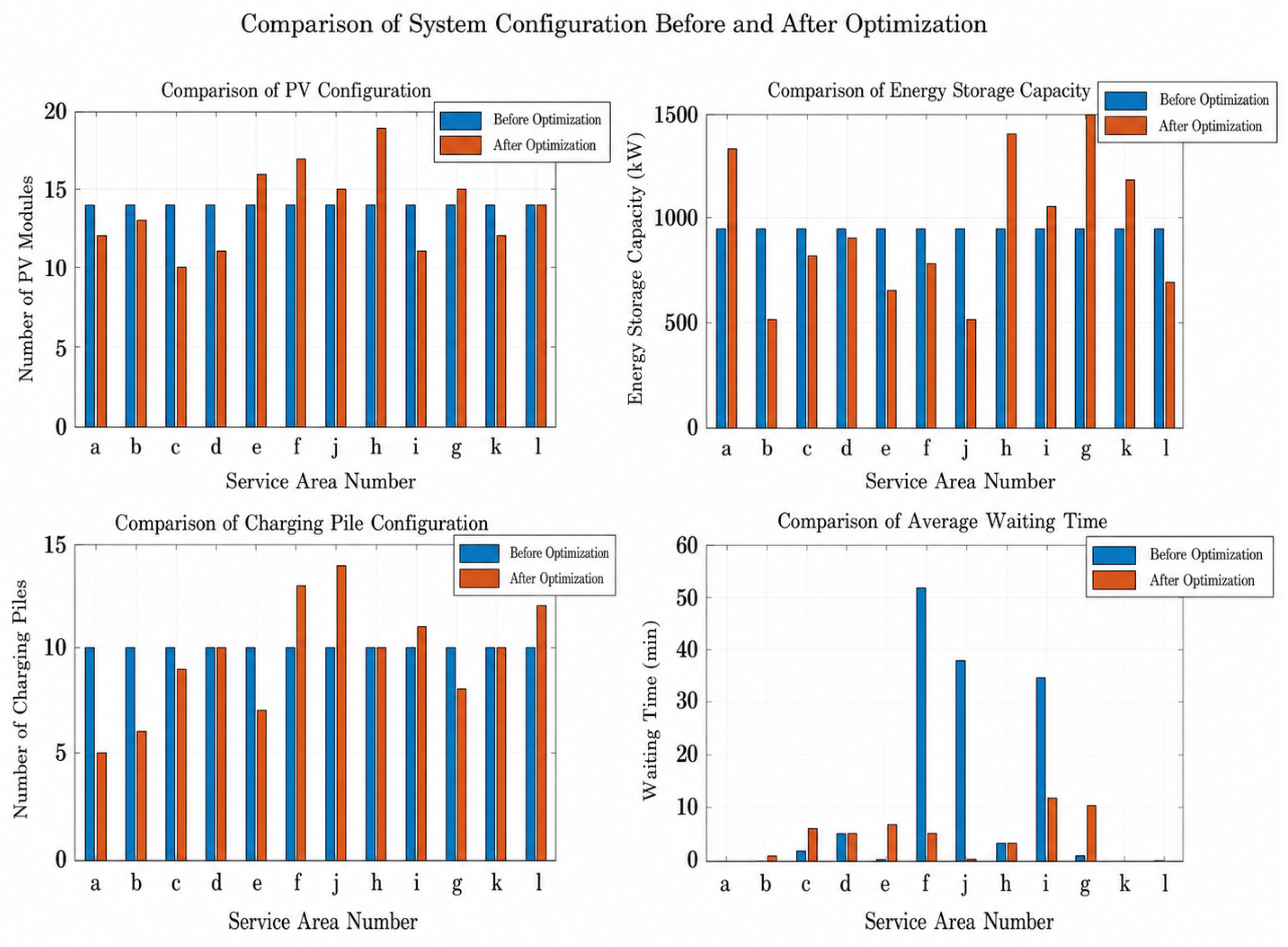
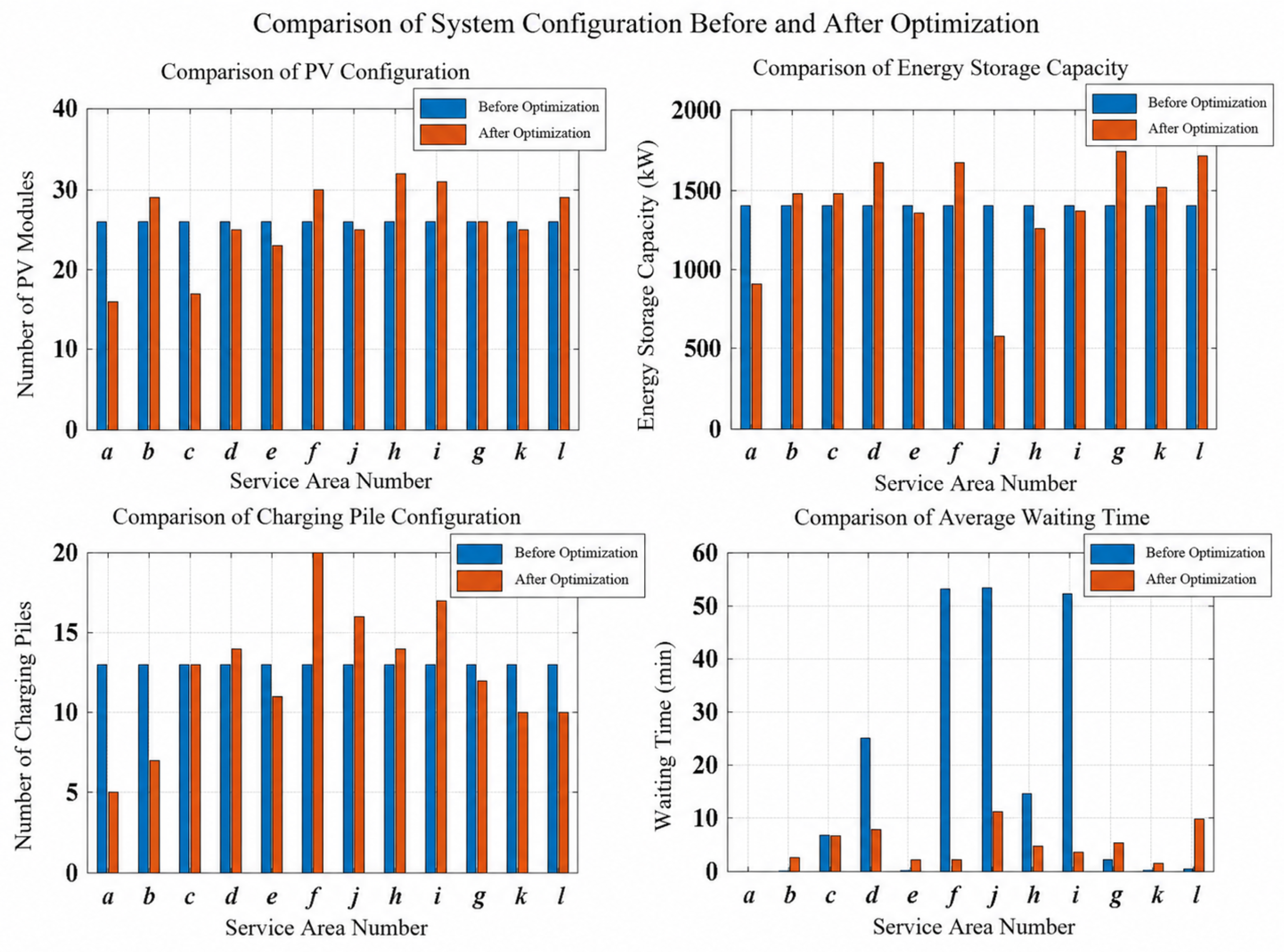
For comparison with the pre-optimization configuration, the average values of the optimized numbers of PV modules and charging piles, as well as the energy storage capacity, are adopted as the benchmark configuration before optimization. A comparison of the relevant variables before and after optimization is presented in Figure 11.

It can be observed that uniformly configuring the equipment at all nodes is unreasonable, as it leads to underutilized resources in low-traffic areas and congestion in high-traffic areas. After optimization, differentiated configurations are adopted according to the variations in traffic flow and charging load at each node, thereby avoiding the resource waste caused by uniform allocation.

The number of PV modules is adjusted according to the local load demand and is significantly increased in the high-load region covering nodes $f$–$h$, thereby reducing the pressure on the power grid. The energy storage capacity is configured in accordance with load fluctuations, with larger capacities assigned to high-load areas to enhance the system’s regulation capability. The optimized allocation of charging piles responds more effectively to charging demand, reducing waiting times in high-traffic areas while avoiding equipment underutilization in low-load areas.

After optimization, the weighted average waiting time of EV users decreases to 5.06 min, while the maximum waiting time among all service areas decreases from 52 min to 11.83 min. Moreover, the penalty value corresponding to $\rho >0.90$ is only 5.52, indicating that the charging-pile configuration is sufficient to accommodate the EV charging demand under the given traffic-flow level.

The optimized configuration reflects a demand-oriented and location-specific allocation strategy. It not only improves equipment utilization efficiency but also significantly enhances the quality of charging services. The economic performance, reliability, and service quality of the system are comprehensively improved, providing a scientific basis for the planning of integrated PV–energy storage–charging systems at highway service areas.

To further validate the effectiveness of the proposed method, following the approach in Ref. [29], EV users’ waiting time is monetized, and a single-objective optimization model is formulated to minimize the sum of the annualized system construction and maintenance costs and the user waiting-time cost. The unit value of users’ waiting time is set to 30% of the average hourly wage. To ensure a fair comparison, except for the objective function, the benchmark model adopts the same traffic demand data, M/M/c queuing model, equipment capacity constraints, and other operational constraints as the proposed model. The results of the single-objective model are compared with those of the proposed VIKOR-M/M/c multi-objective model in

Table 6. Comparison between the proposed multi-objective scheme and the literature-based single-objective scheme under the normal-load scenario.

Indicator	Original Multi-Objective Scheme	Single-Objective Scheme
Global weighted average waiting time	5.0566 min	0.1653 min
Annualized construction cost	2,476,700 RMB/year	3,214,367 RMB/year
Annual maintenance cost	99,068 RMB/year	128,575 RMB/year
Total construction and maintenance cost	2,575,768 RMB/year	3,342,941 RMB/year

.

As shown in Table 6, the single-objective scheme reduces the global weighted average waiting time by deploying more charging piles; however, its total construction and maintenance cost reaches RMB 3,342,941 per year. In contrast, the proposed VIKOR-based multi-objective scheme effectively reduces the total construction and maintenance cost while maintaining the average waiting time within an acceptable range. These results demonstrate that the proposed method can avoid the overdeployment of facilities caused by solely minimizing waiting time and achieve a more reasonable trade-off between system economy and user service quality.

(2)

High-Load Scenario

The high-load scenario is designed to simulate surges in travel demand during holidays or increases in electric vehicle penetration in the future. The predicted charging loads at the service areas under this scenario are shown in Figure 12. Since the two scenarios adopt the same OD traffic-flow distribution and temporal distribution, the spatiotemporal variation patterns of the charging loads under the high-load scenario are generally consistent with those under the normal-load scenario, although the overall load level is substantially higher. Compared with the normal-load scenario, the total system charging load increases by approximately 50%, and the maximum load at an individual node exceeds 1300 kW.

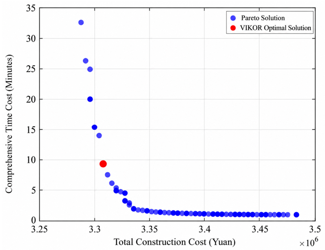
A multi-objective genetic algorithm is employed to optimize the PV–energy storage–charging configuration of the service areas, with the maximum waiting time for EV users constrained to 30 min. The resulting Pareto front is shown in Figure 13. Compared with the normal-load scenario, the increases in investment and waiting time are generally consistent with the growth in charging load.

The Pareto front under the high-load scenario also exhibits a distinct “rapid decline–gradual stabilization” pattern. In the low-cost, high-waiting-time region (upper left), the system investment cost is reduced at the expense of longer waiting times for EV users. The high-cost, low-waiting-time region (lower right) corresponds to relatively sufficient equipment capacity. However, owing to distribution-network power constraints and diminishing marginal benefits, further increases in equipment capacity yield only limited reductions in waiting time. Therefore, the Pareto front gradually stabilizes in this region.

The balanced region near the knee point provides the most favorable investment–benefit trade-off. The optimal solution obtained using the VIKOR method is located near the knee point of the Pareto front, indicating that the corresponding configuration can effectively balance system cost and service quality.

The red dot in Figure 13 represents the optimal solution selected from all non-dominated solutions under the specified weighting coefficient. Under this solution, the construction and maintenance cost is RMB 3.3078 million, and the comprehensive waiting-time cost for EV users is 9.67 min.

Similarly, the average values of the optimized numbers of PV modules and charging piles, as well as the energy storage capacity, are adopted as the direct configuration (i.e., the pre-optimization benchmark). A comparison of the relevant variables before and after optimization is presented in Figure 14. The optimization results show that the weighted average waiting time of EV users decreases to 5.35 min, while the maximum waiting time among all service areas is reduced from 53 min to 12.12 min. In addition, the penalty value corresponding to $\rho >0.90$ is only 12.98, indicating that the charging-pile configuration is appropriate and capable of accommodating the EV charging demand under the given traffic-flow level.

Compared with the configuration under the normal-load scenario, the high-load scenario requires a larger overall system capacity, with notable increases in the numbers of PV modules and charging piles, as well as in energy storage capacity, while maintaining a demand-oriented differentiated configuration strategy.

Based on the optimization results obtained under the two load scenarios, a phased implementation strategy is recommended for engineering construction. During the initial stage, the infrastructure may be configured according to the normal-load scenario, while sufficient distribution-network capacity, equipment interfaces, and construction space should be reserved at high-traffic service areas to accommodate future expansion. For service areas with relatively low charging demand, the initial construction scale may be appropriately limited to avoid long-term equipment underutilization. During operation, the charging and discharging strategy of the energy storage system can be dynamically adjusted according to traffic-flow forecasts. During high-load periods, such as public holidays, mobile charging facilities can be deployed, while vehicle guidance and load-warning measures can be strengthened to alleviate charging pressure at individual service areas. Equipment selection and system design should also account for the operational requirements under both load scenarios to improve the scalability and utilization efficiency of the infrastructure. Overall, the dual-scenario optimization scheme can simultaneously satisfy routine operational requirements and ensure adequate service capacity during peak traffic periods, thereby providing a useful reference for the planning and construction of integrated PV–energy storage–charging systems at highway service areas.

It should be noted that the model developed in this study still involves several simplifications. For modeling convenience, the case study assumes that all EVs have the same battery capacity, energy consumption level, and charging power, and adopts an SOC-based charging probability to describe users’ charging decisions. Therefore, differences arising from vehicle types, driving habits, and user charging preferences are not fully considered. In addition, the charging process is simplified without further considering variations in charging power with SOC or more complex vehicle arrival and charging service processes. Therefore, the results of this study are more applicable to capacity configuration analysis at the planning stage, while there are still limitations in describing detailed real-world operating processes. Future research will further consider the heterogeneity of vehicle parameters and charging behavior and incorporate more comprehensive real-world traffic flow and charging data to improve and validate the model.

7. Conclusions

For the planning of photovoltaic–energy storage–charging integrated systems in highway service areas, this study proposes a capacity configuration model based on multidimensional cost analysis. First, considering the spatiotemporal distribution characteristics of traffic flow, Monte Carlo simulation is employed to dynamically calculate the charging demand of each vehicle according to its state of charge (SOC) at each node, thereby obtaining the spatiotemporal distribution of charging loads at highway service areas. An M/M/c queuing model is further used to calculate the vehicle waiting time. On this basis, a multi-objective optimization model is established by jointly considering the construction and maintenance costs of the highway PV–energy storage–charging system and the comprehensive waiting-time cost of EV users. A multi-objective genetic algorithm is then used to obtain the Pareto front, and the VIKOR decision-making method is introduced to determine the optimal solution.

Under the normal-load scenario, the selected solution has a construction and maintenance cost of RMB 2.5758 million and a comprehensive waiting-time cost of 7.23 min. The weighted average waiting time is 5.06 min, the maximum waiting time is reduced from 52 min to 11.83 min, and the charging-pile overload penalty is 5.52. Under the high-load scenario, the corresponding construction and maintenance cost is RMB 3.3078 million, while the comprehensive waiting-time cost is 9.67 min. The weighted average waiting time is 5.35 min, the maximum waiting time is reduced from 53 min to 12.12 min, and the charging-pile overload penalty is 12.98. Although the daily EV traffic volume increases by 50%, from 4000 to 6000 vehicles, the weighted average waiting time increases by only 0.29 min after capacity reconfiguration, while the maximum waiting time remains at approximately 12 min. These results indicate that the proposed capacity configuration method can accommodate the growth in charging demand through differentiated capacity allocation and expansion without a substantial deterioration in charging service quality.

References

1. Ge, S.Y.; Feng, L.; Liu, H.; Wang, L. Planning of charging stations on highway considering power distribution and driving mileage. Electr. Power Autom. Equip. 2013, 33, 111–116. [Google Scholar] [CrossRef]
2. Zheng, H.; He, X.; Li, Y.; Peeta, S. Traffic equilibrium and charging facility locations for electric vehicles. Netw. Spat. Econ. 2017, 17, 435–457. [Google Scholar] [CrossRef] [Scilit]
3. Liu, K.; Liu, Y. Stochastic user equilibrium based spatial-temporal distribution prediction of electric vehicle charging load. Appl. Energy 2023, 339, 120943. [Google Scholar] [CrossRef] [Scilit]
4. Li, S.B.; Zhu, Y.C.; Tan, J.D.; Kang, Y.Q.; Dong, H.Y. Optimal method for photovoltaic-storage-charging capacity configuration of microgrid-in-chain on expressways considering load spatio-temporal characteristics. Power Syst. Technol. 2025, 49, 2768–2778. [Google Scholar] [CrossRef]
5. Hammam, A.H.; Nayel, M.A.; Mohamed, M.A. Optimal design of sizing and allocations for highway electric vehicle charging stations based on a PV system. Appl. Energy 2024, 376, 124284. [Google Scholar] [CrossRef] [Scilit]
6. Asna, M.; Shareef, H.; Prasanthi, A. Planning of fast charging stations with consideration of EV user, distribution network and station operation. Energy Rep. 2023, 9, 455–462. [Google Scholar] [CrossRef] [Scilit]
7. Kumar, N.; Kumar, T.; Nema, S.; Thakur, T. A comprehensive planning framework for electric vehicles fast charging station assisted by solar and battery based on queueing theory and non-dominated sorting genetic algorithm-II in a co-ordinated transportation and power network. J. Energy Storage 2022, 49, 104180. [Google Scholar] [CrossRef] [Scilit]
8. Meng, F.; Pei, W.; Zhang, Q.; Zhang, Y.; Ma, B.; Li, L. Research on the capacity of charging stations based on queuing theory and energy storage scheduling optimization sharing strategy. J. Energy Storage 2024, 96, 112673. [Google Scholar] [CrossRef] [Scilit]
9. Pourvaziri, H.; Sarhadi, H.; Azad, N.; Afshari, H.; Taghavi, M. Planning of electric vehicle charging stations: An integrated deep learning and queueing theory approach. Transp. Res. Part E Logist. Transp. Rev. 2024, 186, 103568. [Google Scholar] [CrossRef] [Scilit]
10. Rehman, W.U.; Wang, S.; Lv, L.; Kimball, J.W.; Bo, R. Multi-period coordinated planning of XFCS in coupled TN-PDN networks: Integrating demand charge reduction and pre-existing infrastructure. eTransportation 2026, 27, 100521. [Google Scholar] [CrossRef] [Scilit]
11. Yang, N.; Liang, J.Z.; Ding, L.; Zhao, J.H.; Xin, P.Z.; Jiang, J.; Li, Z.H. Integrated optical storage charging considering reconstruction expansion and safety efficiency cost. Power Syst. Technol. 2023, 47, 3557–3569. [Google Scholar] [CrossRef]
12. Liu, J.Y.; Lyu, L.; Gao, H.J.; Liu, J.Y.; Shi, W.C.; Wu, Y. Planning of active distribution network considering characteristics of distributed generator and electric vehicle. Autom. Electr. Power Syst. 2020, 44, 41–48. [Google Scholar]
13. Chaudhari, K.; Ukil, A.; Kumar, K.N.; Manandhar, U.; Kollimalla, S.K. Hybrid optimization for economic deployment of ESS in PV-integrated EV charging stations. IEEE Trans. Ind. Inform. 2018, 14, 106–116. [Google Scholar] [CrossRef] [Scilit]
14. Chen, Y.B.; Tian, H.X.; Liu, Y.X.; Chen, Z.Y.; Li, C.L.; Si, Y.; Bao, Y.T. Robust optimization configuration of photovoltaic-storage-charging integrated system in expressway service area considering demand response of electric vehicles. Proc. CSEE 2025, 45, 1752–1767. [Google Scholar] [CrossRef]
15. Pan, X.; Liu, K.; Wang, J.; Hu, Y.; Zhao, J. Capacity allocation method based on historical data-driven search algorithm for integrated PV and energy storage charging station. Sustainability 2023, 15, 5480. [Google Scholar] [CrossRef] [Scilit]
16. Pazouki, S.; Mohsenzadeh, A.; Ardalan, S.; Haghifam, M.R. Simultaneous planning of PEV charging stations and DGs considering financial, technical, and environmental effects. Can. J. Electr. Comput. Eng. 2015, 38, 238–245. [Google Scholar] [CrossRef] [Scilit]
17. Sechilariu, M.; Molines, N.; Richard, G.; Martell-Flores, H.; Locment, F.; Baert, J. Electromobility framework study: Infrastructure and urban planning for EV charging station empowered by PV-based microgrid. IET Electr. Syst. Transp. 2019, 9, 176–185. [Google Scholar] [CrossRef] [Scilit]
18. Sun, B. A multi-objective optimization model for fast electric vehicle charging stations with wind, PV power and energy storage. J. Clean. Prod. 2021, 288, 125564. [Google Scholar] [CrossRef] [Scilit]
19. Ali, A.; Shaaban, M.F.; Abdelfatah, A. Optimal allocation of autonomous PV-powered fast charging stations for electrified transportation considering traffic dynamics. J. Energy Storage 2024, 99, 113323. [Google Scholar] [CrossRef] [Scilit]
20. Wang, P.; Yuan, J. Adaptive multi-stage planning of electric vehicle charging infrastructure with photovoltaic and energy storage systems: A transportation-aware optimization approach. Appl. Energy 2026, 410, 127517. [Google Scholar] [CrossRef] [Scilit]
21. Chen, D.R. Research and Application of Multi-Time Scale Optimal Scheduling for Highway Isolated Microgrid. Master’s Thesis, Chang’an University, Xi’an, China, 2023. [Google Scholar]
22. Fan, H.; Li, J.H.; Guo, Q. Electric vehicle charging guidance strategy considering user charging decision-making behavior. Electr. Power Eng. Technol. 2023, 42, 23–30. [Google Scholar]
23. Wei, J.Z.; Ma, Z.P. Large-scale electric vehicle charging load forecasting based on Monte Carlo algorithm. Electr. Eng. Technol. 2024, 3, 49–53. [Google Scholar] [CrossRef]
24. Zhu, L.W. Research on Optimal Planning Method of Highway Electric Vehicle Charging Stations Based on Dynamic Traffic Simulation. Master’s Thesis, Tianjin University, Tianjin, China, 2018. [Google Scholar]
25. Zenginis, I.; Vardakas, J.S.; Zorba, N.; Verikoukis, C.V. Analysis and quality of service evaluation of a fast charging station for electric vehicles. Energy 2016, 112, 669–678. [Google Scholar] [CrossRef] [Scilit]
26. Kim, J.; Son, S.-Y.; Lee, J.-M.; Ha, H.-T. Scheduling and performance analysis under a stochastic model for electric vehicle charging stations. Omega 2017, 66, 278–289. [Google Scholar] [CrossRef] [Scilit]
27. Green, L.; Kolesar, P. The pointwise stationary approximation for queues with nonstationary arrivals. Manag. Sci. 1991, 37, 84–97. [Google Scholar] [CrossRef] [Scilit]
28. Huang, J.; Wang, X.L.; Shao, C.C.; Tang, L.; Wang, Y.F. Charging strategy of electric vehicles considering three-phase unbalance mitigation of distribution network with new energy. Power Syst. Technol. 2024, 48, 3663–3672. [Google Scholar] [CrossRef]
29. Nishimwe H., L.F.; Yoon, S.-G. Combined optimal planning and operation of a fast EV-charging station integrated with solar PV and ESS. Energies 2021, 14, 3152. [Google Scholar] [CrossRef] [Scilit]
Figure 1. Architecture of the photovoltaic–energy storage–charging integrated system in a highway service area.
Applsci 16 08672 g001
Figure 2. Probability density distribution of EVs’ initial SOC.
Applsci 16 08672 g002
Figure 3. The relation curve of charging probability with SOC.
Applsci 16 08672 g003
Figure 4. Load calculation process for electric vehicles in the service area based on Monte Carlo.
Applsci 16 08672 g004
Figure 5. The queuing process for electric vehicles.
Applsci 16 08672 g005
Figure 6. System state transition diagram of M/M/c model.
Applsci 16 08672 g006
Figure 7. The main steps of multi-objective optimization based on genetic algorithm.
Applsci 16 08672 g007
Figure 8. Ideal and compromise solutions of the VIKOR method.
Applsci 16 08672 g008
Figure 9. Electric vehicle loads in service areas under conventional load scenarios.
Applsci 16 08672 g009
Figure 10. Pareto frontier for regular-load scenarios.
Applsci 16 08672 g010
Figure 11. Comparison of data before and after optimization for regular-load scenarios.
Applsci 16 08672 g011
Figure 12. Electric vehicle loads in service areas under high-load scenarios.
Applsci 16 08672 g012
Figure 13. Pareto frontier for high-load scenarios.
Applsci 16 08672 g013
Figure 14. Comparison of data before and after optimization for high-load scenarios.
Applsci 16 08672 g014