A Physically Decoupled Deformation Monitoring Framework Incorporating Beta-Distributed Thermal Lag Modeling for Hydraulic Structures

Abstract

Hydraulic structures in navigation–hydropower hubs exhibit complex deformation governed by coupled hydraulic, thermal, and long-term effects, making reliable deformation monitoring challenging. Conventional statistical models are prone to multicollinearity-induced overfitting and elevated false alarm rates, while existing temperature components inadequately characterize delayed thermal responses under large reservoir-level fluctuations. To address these issues, this study proposes an SMT-β deformation monitoring model that integrates separated modeling technology (SMT) with a beta distribution-based temperature formulation. Within a physics-guided sequential modeling framework, long-term deformation trends are first extracted using ICEEMDAN, followed by the development of a beta distribution-based temperature component to characterize lagged thermal effects during stable reservoir-level periods. The hydraulic load component is subsequently identified from the residual deformation, and the total deformation is reconstructed through linear superposition of physically interpretable components. Validation using monitoring data from a 300 m-class super-high arch dam demonstrates that the proposed model achieved the highest prediction accuracy (RMSE = 0.318 mm), reduced the overfitting coefficient to 0.48, and eliminated false alarms. The proposed framework effectively mitigates multicollinearity-induced overfitting while improving the physical interpretability of deformation monitoring, offering a robust and extensible approach for hydraulic structures subjected to complex environmental loads.

1. Introduction

Inland navigation–hydropower hubs are key infrastructures that integrate hydropower generation, flood control, and navigation. During long-term operation, their hydraulic structures are simultaneously subjected to multiple environmental and operational loads, including reservoir water level fluctuations, temperature variations, and navigation-induced disturbances. The coupling of these loads results in highly non-stationary deformation responses with complex temporal characteristics, posing significant challenges to structural health monitoring and safety assessment. Since structural deformation directly reflects the mechanical state and operational safety of hydraulic structures, establishing accurate and physically interpretable deformation monitoring models is of great importance for life-cycle management and the intelligent operation of navigation–hydropower hubs. Nevertheless, existing deformation monitoring models still suffer from multicollinearity-induced overfitting caused by strongly correlated load factors, while their temperature formulations fail to accurately characterize delayed thermal responses under large reservoir-level fluctuations.

Existing deformation monitoring methods can generally be classified into statistical, deterministic, hybrid, and intelligent models. Statistical models remain the most widely adopted approach in engineering practice due to their simplicity and computational efficiency. Since the pioneering hydrostatic–season–time (HST) framework proposed by Tonini [1], numerous extensions have been developed by incorporating state variables, high-water-level effects, and parameter optimization algorithms to improve prediction accuracy under different operating conditions [2,3,4,5,6]. However, these models remain essentially empirical and exhibit limited physical interpretability. Deterministic approaches employ finite element methods (FEM) to simulate structural responses by considering material properties and boundary conditions, providing stronger physical foundations but suffering from high computational costs and difficulties in accurately reconstructing transient temperature fields [7]. Hybrid models attempt to combine the advantages of statistical and deterministic approaches by integrating FEM-derived hydrostatic responses with statistical formulations for other influencing factors [8,9,10]. More recently, intelligent models based on machine learning and deep learning, including LSTM, LSSVM, DenseNet, spatiotemporal learning, clustering techniques, and ensemble learning, have demonstrated remarkable capability in nonlinear prediction [11,12,13,14,15,16,17]. Despite these advances, most existing approaches estimate hydraulic, thermal, and aging effects simultaneously within a unified regression framework. Consequently, strong correlations among explanatory variables inevitably introduce multicollinearity, reduce parameter robustness, and weaken the physical interpretability required for reliable safety evaluation.

Among all influencing factors, temperature becomes the dominant driving force of seasonal deformation after hydration heat has dissipated during the operational stage of hydraulic structures. However, accurately characterizing thermal lag remains challenging because heat conduction causes structural temperatures to respond hysteretically to atmospheric variations. Traditional HST models represent temperature effects using harmonic functions, which cannot capture transient thermal fluctuations or spatially heterogeneous temperature responses [18]. Subsequent studies have improved temperature modeling by incorporating measured temperatures, temperature gradients, thermal lag indicators, and machine-learning-based temperature reconstruction [19,20,21,22,23,24,25,26]. Nevertheless, these methods generally remain embedded within coupled regression frameworks and therefore cannot simultaneously address thermal hysteresis and multicollinearity under fluctuating reservoir conditions, limiting prediction accuracy, model robustness, and the reliability of deformation monitoring [27].

To overcome these limitations, this study proposes an SMT-β deformation monitoring model that integrates separated modeling technology (SMT) with the beta distribution. The proposed framework follows a physically motivated strategy of decoupling deformation mechanisms and independently modeling each component. Specifically, the long-term aging trend is first extracted using Improved Complete Ensemble Empirical Mode Decomposition with Adaptive Noise (ICEEMDAN). Subsequently, the beta distribution is introduced to characterize delayed thermal responses and establish a physically consistent temperature component under quasi-constant hydraulic conditions. Finally, hydraulic deformation is identified from the residual signals after removing the aging and thermal components, thereby avoiding the simultaneous regression of strongly correlated variables. Validation using monitoring data from a 300-m-class ultra-high arch dam demonstrates that the proposed model substantially improves prediction accuracy, enhances parameter stability, and effectively suppresses false alarms. The proposed framework provides a physically interpretable solution for deformation monitoring under multi-load coupling conditions and offers a new strategy for constructing temperature components in hydraulic structure monitoring, thereby supporting the intelligent operation and life-cycle safety management of inland navigation–hydropower hubs.

2. A Deformation Monitoring Model Combining Separable Modeling Technique (Smt) and the Beta Distribution

For deformation monitoring models of hydraulic structures at hydroelectric power stations (such as sluice gates, gravity-type channel protection embankments, etc.), the total deformation is typically composed of three components: hydrostatic pressure, temperature, and time-dependent effects. The expression is as follows [28]:

$$\delta (t)={\delta }_H(t)+{\delta }_{Tem}(t)+{\delta }_{\theta }(t)+a_0$$

(1)

where $\delta (t)$ is the model-estimated deformation response at time t, ${\delta }_H(t)$, ${\delta }_{Tem}(t)$, ${\delta }_{\theta }(t)$ are the hydraulic, thermal, and aging components of the deformation monitoring model, respectively; and $a_0$ is a constant term. Since hydraulic and thermal loads generally exhibit periodic variations, the corresponding hydraulic- and temperature-induced deformations also show cyclic responses and are therefore classified as periodic deformation components. In contrast, aging deformation results from long-term processes such as material creep, consolidation, and foundation compression under the sustained effects of self-weight and material deterioration. It manifests as a gradual and irreversible change over time and is thus regarded as a non-periodic response component.

To eliminate the mutual interference among different deformation components, this study proposes a novel deformation monitoring model for hydraulic structures in navigation–hydropower hubs, termed SMT-β, which integrates separated modeling technology (SMT) with the beta distribution function. The proposed approach first decomposes the measured deformation monitoring data into individual deformation components. Each component is then modeled separately according to its distinct physical characteristics, and the resulting component models are subsequently superimposed to construct the overall deformation monitoring model for hydraulic structures in navigation–hydropower hubs. By decoupling the modeling process of different deformation mechanisms, the SMT-β model aims to fundamentally mitigate the overfitting problem caused by multicollinearity in conventional statistical models, thereby improving both model robustness and interpretability.

2.1. Improved Complete Ensemble Empirical Mode Decomposition with Adaptive Noise (ICEEMDAN)

Dam deformation monitoring data can be viewed as a multi-frequency signal sequence, for which signal-processing techniques provide an effective means of isolating the aging deformation component. Empirical mode decomposition (EMD) is a data-driven approach for analyzing nonlinear and non-stationary signals and has been extensively employed in dam monitoring applications, including signal denoising, seismic signal processing, damage detection, and time-varying feature extraction [29]. By decomposing a time series into a set of intrinsic mode functions (IMFs) and a residual trend component, EMD enables the identification of the aging deformation component. The EMD decomposition process is summarized as follows:

$$\delta \left(t\right)={\displaystyle \sum _{i=1}^{n}IM{F}_i\left(t\right)}+r_n\left(t\right)$$

(2)

where $\delta \left(t\right)$ is the dam deformation monitoring sequence and ${\mathrm{IMF}}_{\mathrm{i}}\left(t\right) (i=1,2,\mathrm{L},n)$ is the ith IMF in the data sequence. $r_n\left(t\right)$ is the lowest-frequency residual sequence, which represents trends in the data—that is, deformation related to the time effect.

As an improved version of EMD, ICEEMDAN employs local mean estimation for mode extraction instead of directly relying on added white noise. This strategy effectively alleviates mode mixing while substantially reducing the interference of white noise during the decomposition process [30]. The implementation procedure of ICEEMDAN is described as follows:

(1) Construct and compute the first residual sequence using EMD:

$$r_1(t)=\langle M{\delta }_i(t)\rangle$$

(3)

(2) Calculate the first intrinsic mode function:

$${IMF}_1^{″}\left(t\right)=\delta \left(t\right)-r_1\left(t\right)$$

(4)

(3) Define the second residual sequence as the mean of $r_1\left(t\right)+{\epsilon }_1{E}_2(W_i(t))$, and obtain the second IMF as:

$${IMF}_2^{″}\left(t\right)=r_1\left(t\right)-r_2\left(t\right)=r_1\left(t\right)-\langle M(r_1\left(t\right)+{\epsilon }_1{E}_2(W_i(t)))\rangle$$

(5)

(4) By repeating steps (2) and (3), the nth residual sequence and the corresponding IMF can be expressed as:

$$r_n(t)=\langle M(r_{n-1}\left(t\right)+{\epsilon }_{n-1}{E}_n(W_i(t)))\rangle$$

(6)

$${IMF}_n^{″}\left(t\right)=r_{n-1}\left(t\right)-r_n\left(t\right)$$

(7)

where $\mathrm{M}(·)$ is the local mean operator, $\langle ·\rangle$ is the ensemble average operator, ${\mathrm{\epsilon }}_{\mathrm{i}}{\mathrm{W}}_{\mathrm{i}}\left(\mathrm{t}\right)$ is a realization of white noise, and ${\mathrm{E}}_{\mathrm{k}}(·)$ is the operator that extracts the kth IMF through EMD.

2.2. Modeling the Temperature Lag Effect Based on the Beta Function

Temperature loading is one of the most significant environmental factors affecting hydraulic structures in navigation–hydropower hubs and can induce substantial structural deformation. Consequently, the characterization of dam temperature fields and the formulation of temperature components in deformation monitoring models have long been important research topics. Existing approaches generally employ approximate representations, such as sinusoidal harmonic functions to describe the periodic variation of temperature fields and moving-average air temperatures to account for the lagged relationship between temperature and deformation. Alternative methods, including Rayleigh distribution functions and Taylor series expansions, have also been proposed to establish temperature–deformation relationships, resulting in improved prediction accuracy to some extent.

Building upon previous studies on the correlation between air temperature and structural deformation, this study proposes a temperature-component modeling approach based on the beta function. The method aims to improve the characterization of temperature-induced deformation when direct temperature measurements within the structure are unavailable. Moreover, it provides a new perspective for investigating the relationship between ambient air temperature and the internal temperature field of hydraulic structures in navigation–hydropower hubs.

2.2.1. Beta Distribution

The beta distribution is a continuous probability distribution defined on the interval [0, 1]. It is characterized by two shape parameters, $\alpha$ and $\beta$, satisfying $\alpha >0$ and $\beta >0$. A random variable x is said to follow a beta distribution if its probability density function is given by:

$$f(x;\alpha ,\beta )={\displaystyle \frac{x^{\alpha -1}{(1-x)}^{\beta -1}}{{\displaystyle {\int }_0^1{x}^{\alpha -1}{(1-x)}^{\beta -1}dx}}} ={\displaystyle \frac{x^{\alpha -1}{(1-x)}^{\beta -1}}{{\displaystyle {\int }_0^1{u}^{\alpha -1}{(1-u)}^{\beta -1}du}}} ={\displaystyle \frac{1}{B(\alpha ,\beta )}}{x}^{\alpha -1}{(1-x)}^{\beta -1}$$

(8)

where $\alpha$ and $\beta$ are the shape parameters, and $B(\alpha ,\beta )$ is the beta function.

The shape of the beta distribution is governed by the values of $\alpha$ and $\beta$:

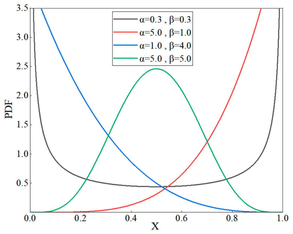
(1) When $0<\alpha <1$ and $0<\beta <1$, the distribution is a trend of first decreasing and then increasing. The curve is concave on the interval (0, 1), and as x approaches 0 or 1, $f(x)\to \infty$.

(2) When $0<\alpha <1$ and $\beta \ge 1$, the distribution is a decreasing trend. The curve continues downward, and as $x\to 0$, then $f(x)\to \infty$, as $x\to 1$, then $f(x)\to 0$.

(3) When $\alpha \ge 1$ and $0<\beta <1$, the distribution is an upward trend. The curve continues to rise, and as $x\to 0$, then $f(x)\to 0$, as $x\to 1$, then $f(x)\to \infty$.

(4) When $\alpha \ge 1$ and $\beta \ge 1$, the distribution is a trend of first increasing and then decreasing. The curve takes the form of a single peak, and as $x\to 0$, then $f(x)\to 0$, as $x\to 1$, then $f(x)\to 0$.

It can be seen that different combinations of the shape parameters $\alpha$ and $\beta$ produce substantially different distribution forms. Figure 1 illustrates four representative beta distributions, highlighting the remarkable flexibility of the beta distribution in representing a wide variety of functional shapes. This versatility makes it particularly suitable for fitting the diverse distribution patterns encountered in engineering applications.

2.2.2. Heat Conduction Process of Hydraulic Structures

The internal concrete temperatures of hydraulic structures in navigation–hydropower hubs result from the cumulative transfer of heat from the ambient environment. Due to the thermal properties of concrete and the finite heat conduction rate, the internal temperature response exhibits a lag effect relative to ambient air temperature. To investigate this temperature-lag mechanism, the heat conduction process within the structure is derived.

According to the principle of energy conservation and the classical theory of heat transfer in mass concrete, the governing heat conduction equation can be written as [31]:

$$c\rho {\displaystyle \frac{\partial T}{\partial t}}=\lambda ({\displaystyle \frac{{\partial }^{2}T}{\partial x^2}}+{\displaystyle \frac{{\partial }^{2}T}{\partial y^2}}+{\displaystyle \frac{{\partial }^{2}T}{\partial z^2}})+Q=\nabla ·(\lambda ·\nabla T)+Q=\lambda ·{\nabla }^{2}T+Q$$

(9)

$$\nabla =({\displaystyle \frac{\partial }{\partial x}},{\displaystyle \frac{\partial }{\partial y}},{\displaystyle \frac{\partial }{\partial z}})$$

(10)

where c is the specific heat capacity, kJ/(kg∙°C); $\rho$ is the density, kg/m³; T is the dam temperature, °C; t is the time, h; $\lambda$ is the thermal conductivity, kJ/(m∙h∙°C); Q is the heat source term; when the heat of hydration is neglected, $Q=0$; $\nabla$ is the differential operator.

Assuming that the thermal conductivity is constant, the one-dimensional problem can be expressed as:

$${\displaystyle \frac{\partial T}{\partial t}}=a{\displaystyle \frac{{\partial }^{2}T}{\partial x^2}}$$

(11)

$$a={\displaystyle \frac{\lambda }{c\rho }}$$

(12)

where a is the thermal conductivity, ${\mathrm{m}}^2/\mathrm{h}$.

Due to the thermal inertia of concrete, the temperature response of a hydraulic structure at time t is governed not only by the instantaneous temperature load, but also by the cumulative effects of past temperature loads. The influence of historical temperature loads can be quantified by an impulse response (weighting) function, which assigns different weights to temperature inputs at different times. Accordingly, the internal temperature response to ambient air temperature can be represented as the convolution of the external temperature signal and the impulse response function:

$$T(t)=P(t)\ast T_a(t)={\displaystyle {\int }_{-\infty }^t{T}_a(t^{\prime })}·P(t-t^{\prime }){dt}^{\prime }$$

(13)

where ∗ is the convolution operator, $P(t)$ is the impulse response function, and $T_a$ is the ambient air temperature, °C.

According to Equation (12), the internal temperature of the structure at a given time $t_0$ can be estimated as the cumulative effect of ambient air temperatures prior to that instant. In practical applications, the convolution between the ambient temperature and the impulse response function generally falls within the range $\left[t_0-m·T_0, t_0\right]$:

$$T(t_0)={\displaystyle {\int }_{t^{\prime }=t_0-m·T_0}^{t^{\prime }=t_0}{T}_a(t^{\prime })}·P(t_0-t^{\prime }){dt}^{\prime }$$

(14)

where $T\left(t_0\right)$ is the internal temperature of the structure at time $t_0$, $t_0-m·T_0$ is the earliest time at which the ambient temperature still exerts a lagged influence on the structural temperature at time $t_0$, $T_0$ is the length of the time intervals within the influence period, and the coefficient m is determined by $T_0$.

The integral in Equation (13) can be approximated as:

$$T(t_0)={\displaystyle \frac{{\displaystyle {\sum }_{i=t_0-m·T_0}^{i=t_0-1}P(t_0-i)·}{T}_a(i)·\Delta t}{{\displaystyle {\sum }_{i=t_0-m·T_0}^{i=t_0-1}P(t_0-i)}·\Delta t}}$$

(15)

where $\Delta t$ is the length of the summation interval corresponding to the time interval $T_0$.

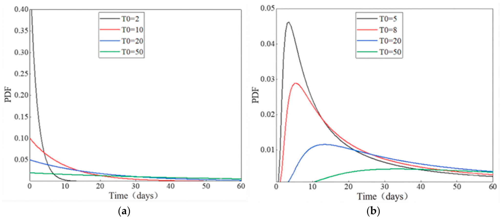
The impulse response function [32] typically takes the following two forms, as shown in Figure 2:

(1) The temperature measurement point is located close to the dam surface:

$$P(t)={\displaystyle \frac{1}{T_0}}·e^{{\displaystyle \frac{-t}{T_0}}}$$

(16)

(2) The temperature measurement point is located deep within the dam, at a considerable distance from the dam surface:

$$P(t)=\sqrt{{\displaystyle \frac{T_0}{\pi }}}·{\displaystyle \frac{e^{-T_0/t}}{t^{3/2}}}$$

(17)

where $T_0$ is the number of days of lag in the effect of the ambient temperature on the measurement points inside the dam.

It can be seen that $\mathrm{P}\left(\mathrm{t}\right)$ generally exhibits two typical forms. In principle, $\mathrm{P}\left(\mathrm{t}\right)$ can be determined once the lag duration ${\mathrm{T}}_0$ is known. However, because different monitoring points are subject to varying influences from environmental factors such as ambient temperature and reservoir water level, their lag characteristics and lag durations differ significantly. Moreover, the distance of a monitoring point from the structural surface is often difficult to quantify precisely. Consequently, determining an appropriate lag duration ${\mathrm{T}}_0$ for each monitoring point is challenging, limiting the practical applicability of conventional impulse response functions.

As discussed in the previous section, the beta distribution is highly flexible and can represent a wide variety of functional forms over the interval [0, 1] through appropriate adjustment of its shape parameters. Notably, it is capable of reproducing both typical forms of the impulse response function $\mathrm{P}\left(\mathrm{t}\right)$. Therefore, the beta probability density function is adopted herein as a substitute for $\mathrm{P}\left(\mathrm{t}\right)$ to characterize the lagged influence of ambient air temperature on the internal temperature response of the structure. To this end, the lag period is first normalized to the interval [0, 1], and the corresponding parameters $\alpha$ and $\beta$ are then identified through optimization.

2.2.3. Development of a Dam Body Temperature Model Based on the Beta Function

To fully capture the influence of ambient air temperature on the internal temperature field, a sufficiently long temperature history (150 days) was considered in this study to model the temperatures at different locations within the dam. Physically, massive concrete has a low thermal diffusivity, resulting in a significant time lag in the response of its internal temperature to changes in boundary air temperature. Therefore, a period of 150 days (approximately 5 months) was selected to provide a sufficiently long window for capturing the dominant delayed thermal response. By combining the beta distribution with ambient air temperature, the internal temperature can be expressed as follows:

$$T\left(t_1\right)={\displaystyle {\int }_{t^{\prime }=t_1-t^{\ast }}^{t^{\prime }=t_1}{T}_i^{\prime }(t\prime )}·Beta(t^{\prime })$$

(18)

where $\mathrm{T}\left(t_1\right)$ is the estimated value of the dam body temperature at time t₁; $t^{\ast }$ is the duration of the effect of ambient temperature on the dam body thermometer; in this paper, we used data from the 150 days preceding time t₁, i.e., we set $t^{\ast }=150$; ${\mathrm{T}}_i^{\prime }\left(t^{\prime }\right)$ is the ambient temperature at time $t^{\prime }$; $\mathrm{Beta}\left(t^{\prime }\right)$ is the beta impact function at time $t^{\prime }$.

The above equation can be approximated as the sum of the product of the average temperature and its corresponding weight:

$$T\left(t_1\right)={\displaystyle \frac{{\displaystyle {\sum }_{i=t_1-t^{\ast }}^{i=t_1}{T}_i^{\prime }(i)Beta(i)}\ast \Delta t}{{\displaystyle {\sum }_{i=t_1-t^{\ast }}^{i=t_1}Beta(i)}\ast \Delta t}}$$

(19)

where $\Delta t$ is the number of days in a unit of time, $\Delta t=1$.

The determination of the optimal shape parameters is cast as an optimization problem. Owing to their strong global search capability, intelligent optimization methods, including neural networks, particle swarm optimization, the Levenberg–Marquardt algorithm, genetic algorithms, and general global optimization techniques, have been widely employed for parameter calibration in monitoring models. Here, the objective function is defined as the sum of squared relative errors between the measured and predicted temperatures:

$$E=\min \left\{{{\displaystyle {\sum }_{i=1}^m\left(\frac{T_i^{\ast }(t)-T_i\left(t_1,t_2,\cdots ,t_m\right)}{T_i^{\ast }(t)}\right)}}^2\right\}$$

(20)

where ${\mathrm{T}}_i^{\ast }(t\left)\right(i=1,2,\cdots ,m)$ is the reading from the dam body thermometer at time t; ${\mathrm{T}}_{\mathrm{i}}\left(t_1,t_2,\cdots ,t_{\mathrm{m}}\right)$ is the estimated value of the dam’s temperature at time t; m is the length of the temperature monitoring data series to be fitted.

A genetic algorithm is employed to determine the optimal solution of the objective function, yielding the optimal parameter set ($\alpha$, $\beta$), which characterizes the lagged influence of ambient temperature on different monitoring locations.

2.2.4. Constructing the Temperature Component Model Based on the Beta Function

The relationship between ambient air temperature and the internal dam temperature is modeled using a beta distribution, whose parameters are optimized to characterize the heat-transfer process. Considering the strong correlation between dam deformation and temperature, an equivalent dam temperature was derived from the 150-day air-temperature history using the beta-distribution-based model and subsequently adopted as the governing variable for the temperature component, expressed as follows:

$${\delta }_{Tem}=mT\left(t\right)={\displaystyle \frac{m · {\displaystyle {\sum }_{i=t-t^{\ast }}^{i=t}{T}_i^{\prime }(i)Beta(i)}\ast \Delta t}{{\displaystyle {\sum }_{i=t-t^{\ast }}^{i=t}Beta(i)}\ast \Delta t}}$$

(21)

where ${\mathsf{\delta }}_{\mathrm{Tem}}$ is the temperature component of the deformation at the monitoring point at time t; n is the duration, set $n=150$; $\mathrm{Beta}(i)$ is the beta weight corresponding to the atmospheric temperature i days before time t; ${\mathrm{T}}_{\mathrm{i}}^{\prime }(\mathrm{i}=1,2,\cdots ,n)$ is the ambient temperature two days prior to time t; ${\mathrm{t}}^{\ast }$ is the duration of the effect of ambient temperature on the dam body thermometer. This study used data from the 150 days prior to time t, ${\mathrm{t}}^{\ast }=150$.

Following the principle of incremental inversion, an objective function is constructed as the sum of squared relative errors between the observed temperature-induced deformation increments and the corresponding increments simulated by the beta distribution, expressed by:

$$E=\min \left\{{{\displaystyle {\sum }_{i=1}^n\left(\frac{\Delta {\delta }_i^{\ast }-\Delta {\delta }_i}{\Delta {\delta }_i^{\ast }}\right)}}^2\right\}$$

(22)

where $\Delta {\mathrm{\delta }}_{\mathrm{i}}^{\ast }(\mathrm{i}=1,2,\cdots ,\mathrm{n})$ is the temperature-induced deformation increment at equal water levels, obtained by applying the condition of equal water levels; $\Delta {\mathsf{\delta }}_i (\mathrm{i}=1,2,\cdots ,\mathrm{n})$ is the temperature deformation increment obtained by fitting the beta distribution corresponding to $\Delta {\mathsf{\delta }}_{\mathrm{i}}$; n is the number of temperature deformation groups obtained under constant water level conditions. It should be noted that if the denominator Δδ_i* is close to zero, using relative error may lead to numerical instability. Although this situation did not arise in this case study, for broader applications, if the observed deformation increments Δδ_i* tend toward zero, the objective function will dynamically switch from the sum of squares of relative errors to the sum of squares of errors to ensure the robustness of parameter optimization.

It should be emphasized that the parameters of the beta impact function B(t), including α, β, and m, and the resulting curve shapes are not subjectively pre-defined. Instead, they are determined through a data-driven fitting process. By taking the actual temperature-induced deformation extracted using the ICEEMDAN algorithm under constant-water-level conditions as the fitting target, an optimization algorithm is employed to minimize the objective function in Equation (22). Through this process, the optimal parameter set that best represents the actual thermal lag characteristics of the dam is iteratively calculated.

2.3. Hydraulic Component Modeling

Structural deformation is generally considered to be power-law dependent on the upstream reservoir water level. Accordingly, the hydraulic component of the deformation monitoring model is typically expressed as a polynomial function of water depth. Since the influence of the downstream water level is often negligible when the downstream depth is small, only the upstream reservoir water level was considered in the present study [33]:

$${\delta }_H(t)={\displaystyle \sum _{i=1}^m{a}_{ui}{H}_u^i}(t)$$

(23)

where ${\delta }_H(t)$ is the estimated value of the water pressure; $a_{ui}(i=1,2,\cdots ,m)$ is the regression coefficient for the upstream water level factor; $H_u^i(t)(i=1,2,\cdots ,m)$ is the ith power of the upstream water level; m is the highest power of the upstream water level factor. For concrete gravity dams and concrete arch dams, m is taken to be 3 and 4, respectively.

The water depth downstream of the dam remains at a relatively high level throughout the year, so the effects of both upstream and downstream water depths must be taken into account:

$${\delta }_H(t)={\displaystyle {\displaystyle \sum _{i=1}^m}{a}_{ui}{H}_u^i(t)}+{\displaystyle {\displaystyle \sum _{j=1}^n}{a}_{dj}{H}_d^j}(t)$$

(24)

where $a_{dj}(j=1,2,\cdots ,n)$ is the regression coefficient for the downstream water level factor; $H_d^j(t)(j=1,2,\cdots ,n)$ is the jth power of the water depth downstream; n is the highest power of the downstream water level factor. For gravity dams and arch dams, n is taken to be 3 and 4, respectively.

For cases with relatively high downstream water levels, where the deformation response exhibits a significant lag effect with respect to reservoir water-level fluctuations, the hydraulic component can be further expressed as a function of the average downstream water level during the k days preceding the observation time:

$${\delta }_H(t)={\displaystyle {\displaystyle \sum _{i=1}^m}{a}_{ui}{H}_u^i}(t)+{\displaystyle {\displaystyle \sum _{j=1}^n}{a}_{dj}{H}_d^j}(t)+{\displaystyle {\sum }_k{a}_k^{\prime }{\overline{H}}_{dk}}(t)$$

(25)

where $a_k^{\prime }$ is the regression coefficient for the average downstream water level factor; ${\overline{H}}_{dk}(t)(k=5,10,15,60)$ is the average downstream water level for the 5, 10, 15, and 60 days preceding the monitoring date.

In deterministic or hybrid models, the design values of the physical and mechanical properties of dam and foundation materials are adopted in finite element analyses to simulate deformation responses under various reservoir water levels. A polynomial power function is first used to characterize the relationship between hydraulic load and deformation response, after which its coefficients are calibrated using field-monitored deformation data:

$${\delta }_H(t)=\alpha {\displaystyle \sum _{i=1}^m{a}_i{H}^i(t)}$$

(26)

where ${\delta }_H(t)$ is the estimated value of the water pressure component; α is the polynomial correction coefficient for the water level factor.

In conventional hybrid models, a correction coefficient is introduced into the hydraulic component to compensate for discrepancies between the assumed and actual material parameters, thereby minimizing the overall fitting error. However, the physical significance remains unclear. To overcome this limitation, some researchers have employed polynomial response surfaces of material parameters to approximate the hydraulic deformation responses obtained from finite element analyses. Combined with parameter inversion techniques, this approach enables the estimation of actual material properties and provides a more realistic representation of the relationship among hydraulic deformation, material parameters, and reservoir water level:

$${\delta }_H(t)=\left({\displaystyle {\displaystyle \sum }_{i=1}^m}{b}_i{x}_i+{\displaystyle {\displaystyle \sum }_{i=1}^m}{c}_i{x}_i^2+{\displaystyle {\displaystyle \sum }_{i=1}^m}{d}_i{x}_i^3\right)\ast {\displaystyle {\displaystyle \sum }_{j=1}^n}{e}_j{H}^j(t)$$

(27)

where $a_i,b_i,c_i(i=1,2,\cdots ,m)$ are the regression coefficients of the material parameters multiplied by the power factors, respectively; $x_i(i=1,2,\cdots ,m)$ is the physical and mechanical properties of different materials; $H^j(t)(j=1,2,\cdots ,n)$ is the jth power of the water depth; m is the number of material parameters selected; n is the highest power of the water level factor, with n = 3 for gravity dams and n = 4 for arch dams.

To mitigate the scaling disparity among model coefficients arising from large water-depth values, the water level is commonly normalized as follows:

$$h(t)={\displaystyle \frac{H(t)-H_{\min }}{H_{\max }-H_{\min }}}$$

(28)

where h(t) is the normalized water level at time t; H(t) is the water level at time t; H_max and H_min are typically the historical maximum water level and the historical minimum water level, respectively.

2.4. Separated Modeling Technique (SMT)

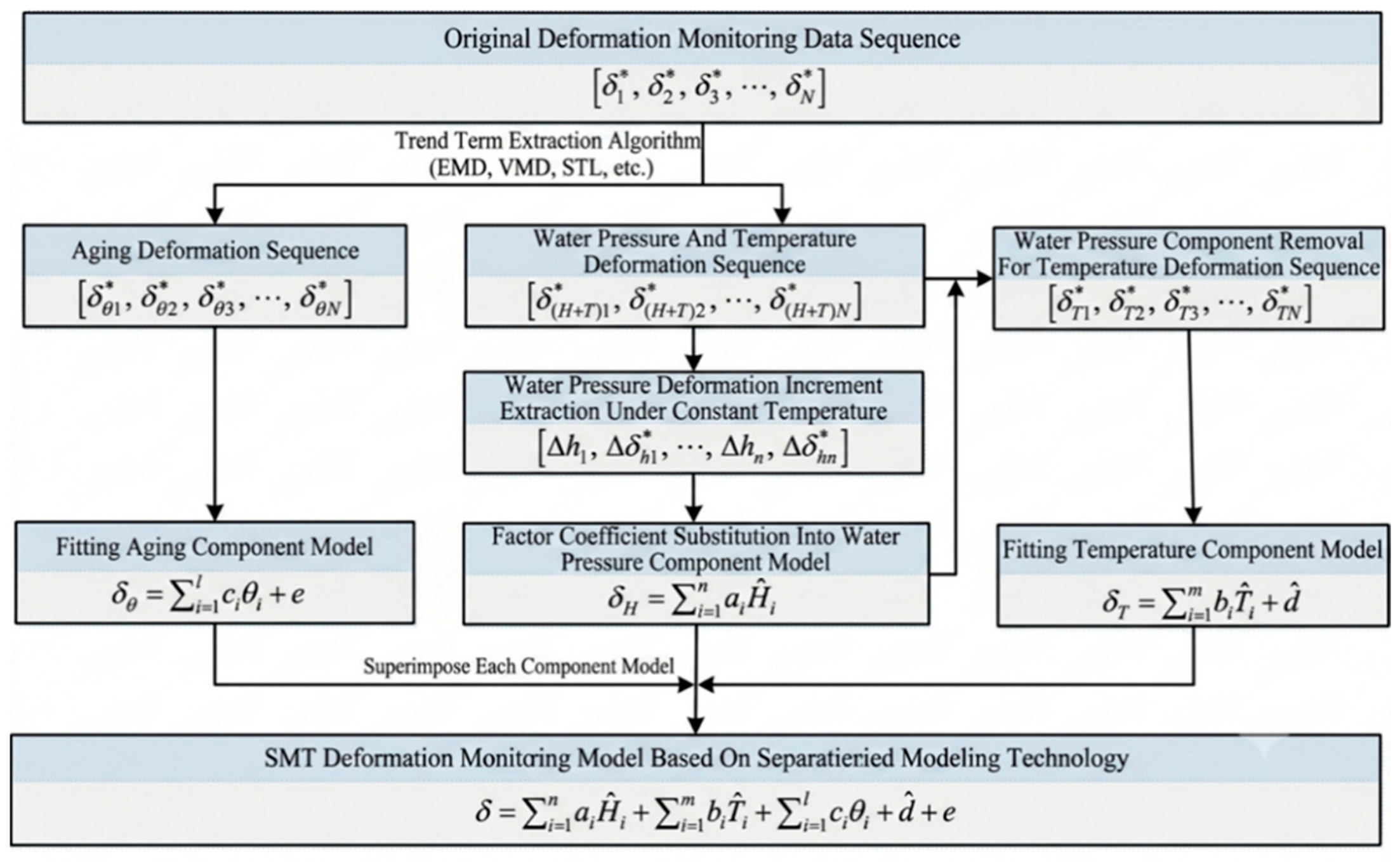
The separated modeling technique (SMT) extends the semi-separated modeling framework by further decoupling hydraulic- and temperature-induced deformations, thereby enabling the independent construction of mathematical models for each deformation component. The key advantage of SMT lies in its decomposition and separate modeling of individual deformation effects, which eliminates mutual interference and compensation among load-related factors. As a result, the risk of overfitting in deformation monitoring models can be effectively reduced.

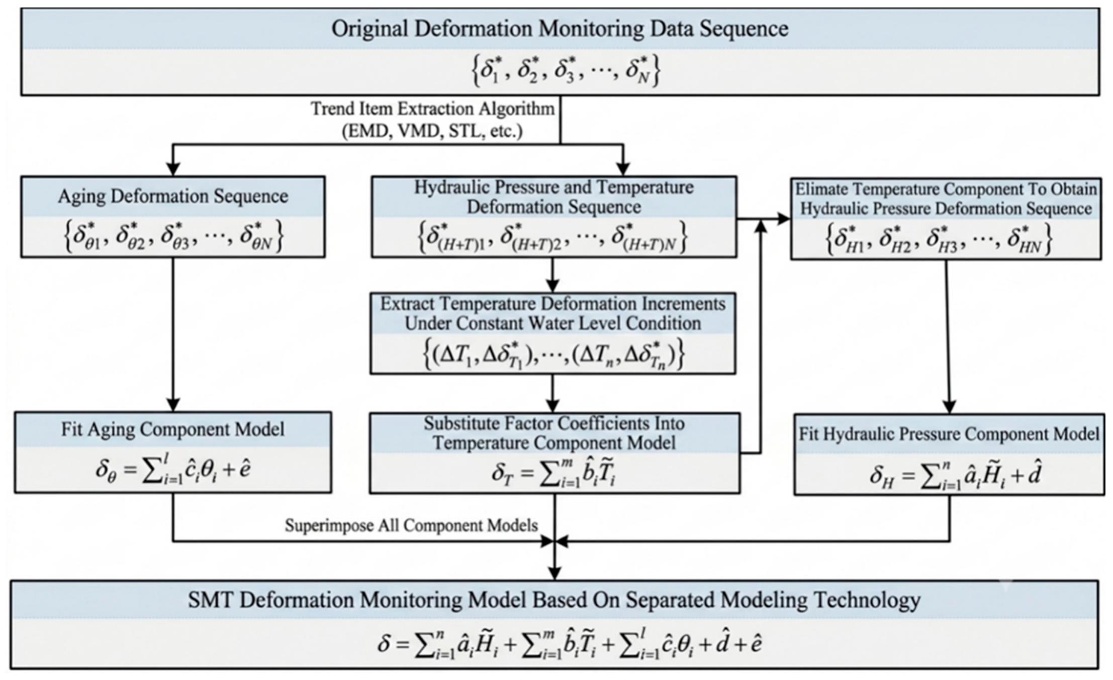
The main procedure of SMT is summarized as follows:

(1) An aging-component separation algorithm is applied to the original deformation monitoring series to extract the long-term deformation trend, from which the aging component model is established.

(2) Under the equal-water-level condition, multiple data groups with identical hydraulic components but different temperature components are extracted from the residual deformation series. The coefficients of the temperature model are then determined by fitting deformation increments induced by temperature variations. Typical temperature factors include moving-average temperature factors, seasonal harmonic factors, and temperature principal components. Alternatively, when sufficient internal temperature measurements are available, data groups with identical temperature components but different hydraulic components can be selected under the equal-temperature condition, and the coefficients of the hydraulic model (e.g., water-level polynomial factors or response surfaces) can be identified by fitting hydraulic deformation increments.

(3) If the equal-water-level condition is adopted in step (2), the remaining deformation series is fitted using the predefined hydraulic-component formulation. Conversely, if the equal-temperature condition is employed, the remaining deformation series is fitted using the temperature-component formulation.

(4) Finally, all independently established deformation components are superimposed to construct the SMT-based deformation monitoring model for the concrete dam.

The workflows of SMT based on the equal-water-level condition and the equal-temperature condition are illustrated in Figure 3 and Figure 4, respectively.

The conventional global-fitting strategy in deformation monitoring models often results in mutual compensation among the hydraulic, thermal, and aging factors. The proposed separated modeling technique (SMT) follows the principle of physical-mechanism decoupling and stepwise independent modeling: aging-effect decoupling—first, the long-term aging trend is extracted from the original deformation time series using the ICEEMDAN algorithm and independently fitted with an exponential function; temperature-effect decoupling—after removing the aging component, deformation increments driven purely by temperature are selected under the equal-water-level condition (ΔH < 0.02 m), and the coefficients of the temperature component are independently calibrated using the computed beta-distribution influence weights; hydraulic-effect decoupling—after further removing the temperature component, a power-polynomial response model is established for water depth using the residual series. Finally, the three physically interpretable, independently modeled components are linearly superimposed to construct the complete SMT-β deformation monitoring model.

3. Case Study

To evaluate the applicability of the model to complex concrete structures, this study used the JP double-curvature arch dam as a case example, applying the separated modeling technique (SMT) to develop deformation monitoring models for vertical-section measurement points. An innovative approach is introduced for the temperature component by employing a beta-distribution-based modeling method, which is then compared with traditional modeling approaches.

3.1. Overview of the JP Arch Dam Project

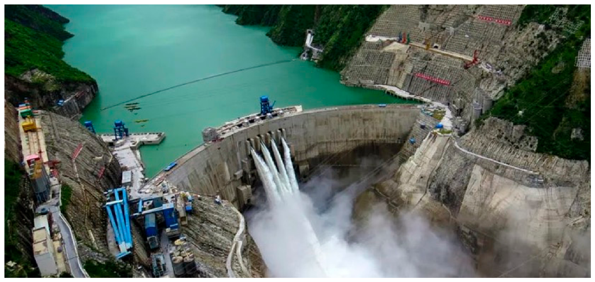
The JP Hydropower Station is a 300 m-class, ultra-high double-curvature arch dam with a normal reservoir water level of EL 1880 m, a dead water level of EL 1800 m, a total storage capacity of 7.76 billion m³, and a regulation capacity of 4.91 billion m³, providing annual flow regulation. The dam consists of 26 segments, with a crest centerline arc length of 552.23 m and a maximum central angle of 93.12°. The dam crest elevation is EL 1885 m, the maximum dam height is 305 m, the crest width is 16 m, the base width is 63 m, and the thickness-to-height ratio is 0.207. An aerial view of the JP hydroelectric power station is shown in Figure 5.

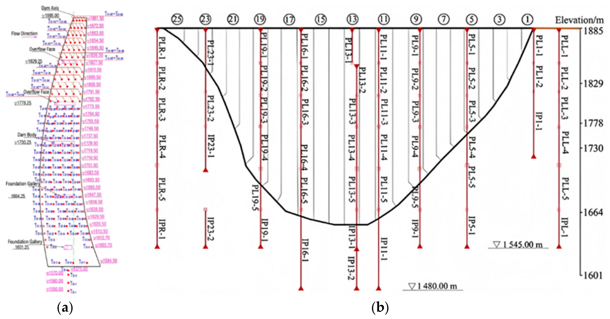
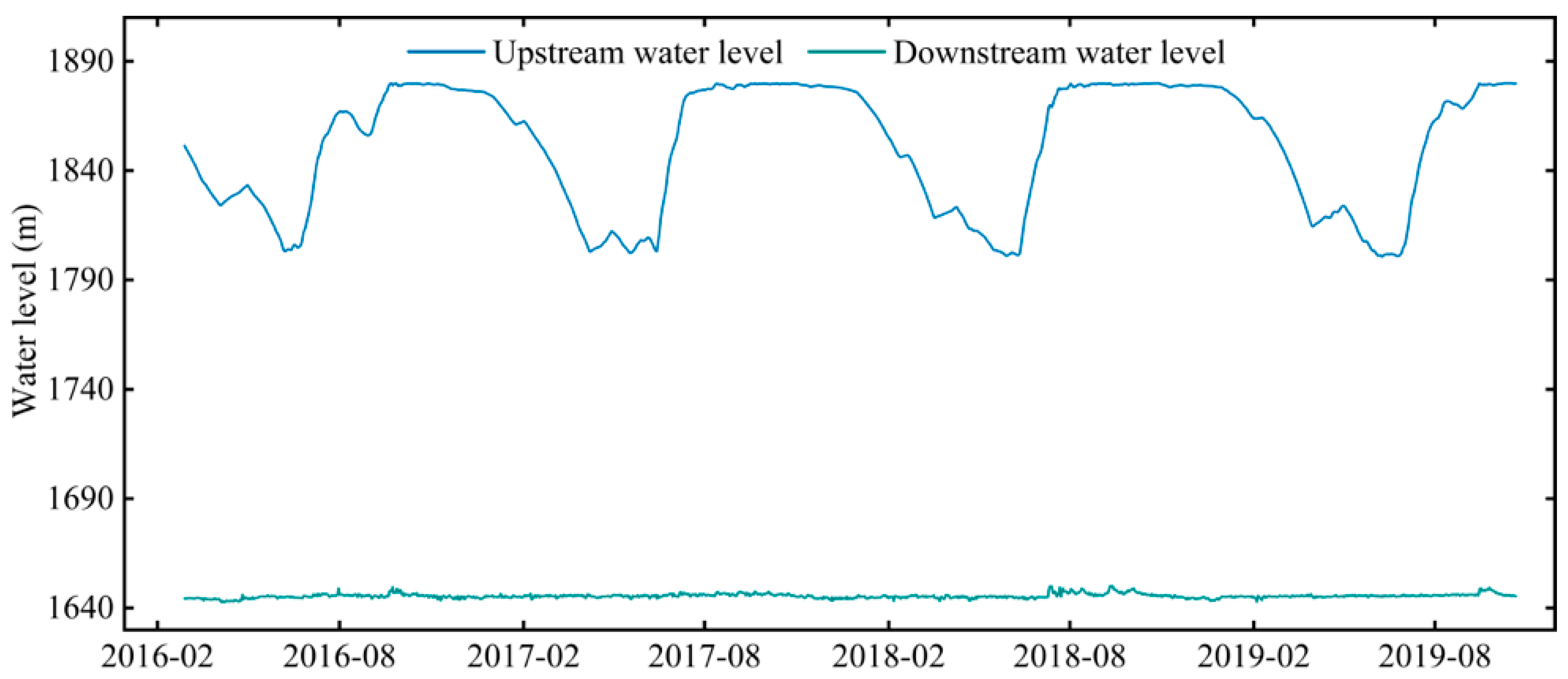
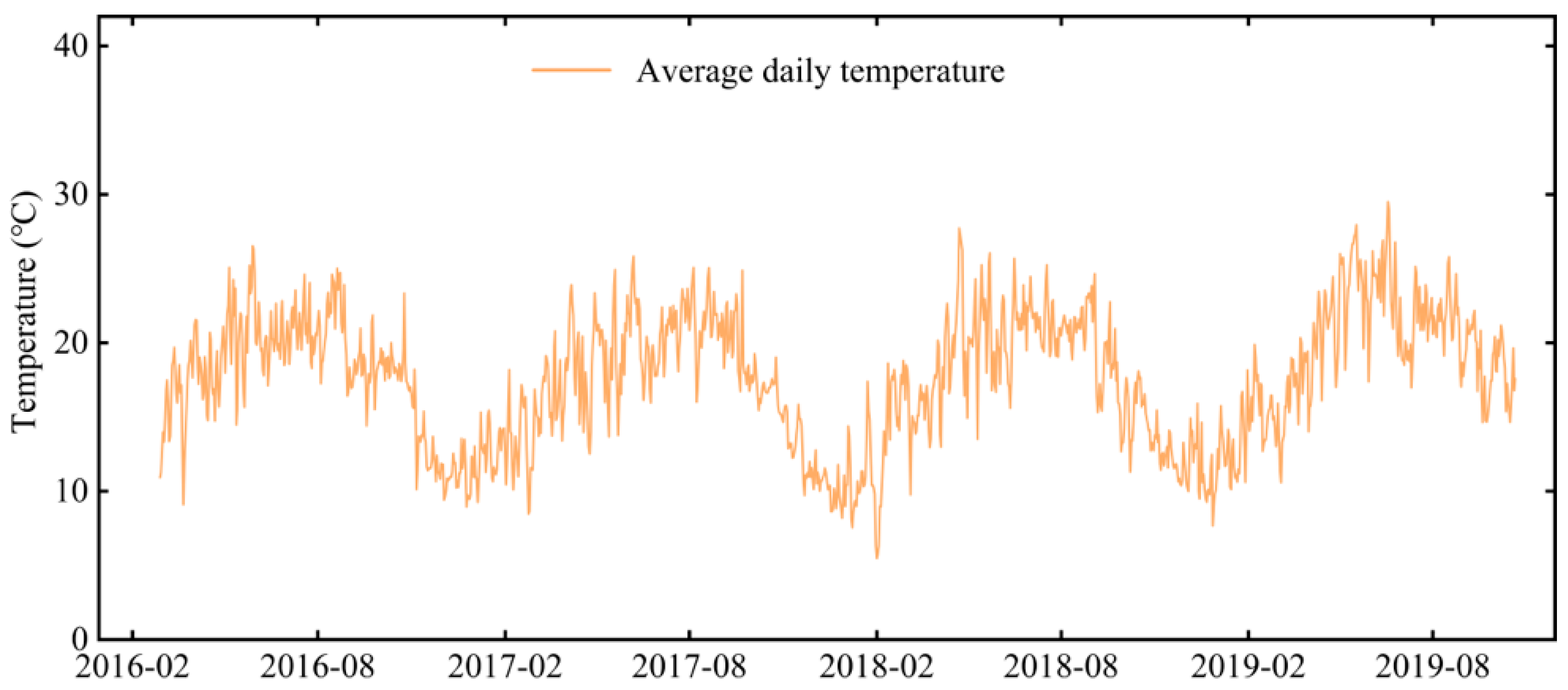
This study focused on the radial displacement of the crest verticals in the left #13 dam segment, where internal temperature measurements are available. Two temperature sensors are installed at elevations 1603.70 m and 1612.70 m: one located 10 cm from the upstream concrete surface and one 10 cm from the downstream surface. Between elevations 1620.50 m and 1881.50 m, five sensors are installed every 9 m: one 10 cm from the upstream surface, one 10 cm from the downstream surface, and three within the dam body, as shown in Figure 6a. Horizontal dam displacements are monitored using forward and reverse verticals, with measurement points arranged as shown in Figure 6b; a total of seven points are installed in the #13 segment. Complete displacement monitoring data for each vertical were collected from 2 September 2016, to 23 October 2019, at a measurement frequency of once per day. The time histories of the upstream and downstream water levels and daily average air temperatures for the dam site are presented in Figure 7 and Figure 8, respectively.

Water levels upstream fluctuate significantly throughout the year, while those downstream remain largely stable. Between 2 September 2016, and 23 October 2019, the highest and lowest water levels upstream were 1879.98 m and 1800.65 m, respectively, with a maximum daily variation of 4.69 m. Downstream water depths remained around 1645 m, with minimal variation.

Air temperatures in the dam area of the JP Hydropower Station exhibit distinct, regular annual cycles, with a certain time lag between temperature changes and vertical displacement. From 2016 to 2020, the daily average temperature ranged from 4.52 °C to 29.50 °C; the time-series curve of daily average temperature changes in the dam area is shown in Figure 8.

3.2. Deformation Monitoring Model for Arch Dams Based on Decomposition Modeling Techniques

3.2.1. Separation and Construction of the Time-Dependent Component

The displacements of vertical measurement points at three different elevations in the #13 dam segment were decomposed, and the aging-related deformation was extracted using the improved Complete Ensemble Empirical Mode Decomposition with Adaptive Noise (ICEEMDAN), as shown in Figure 9.

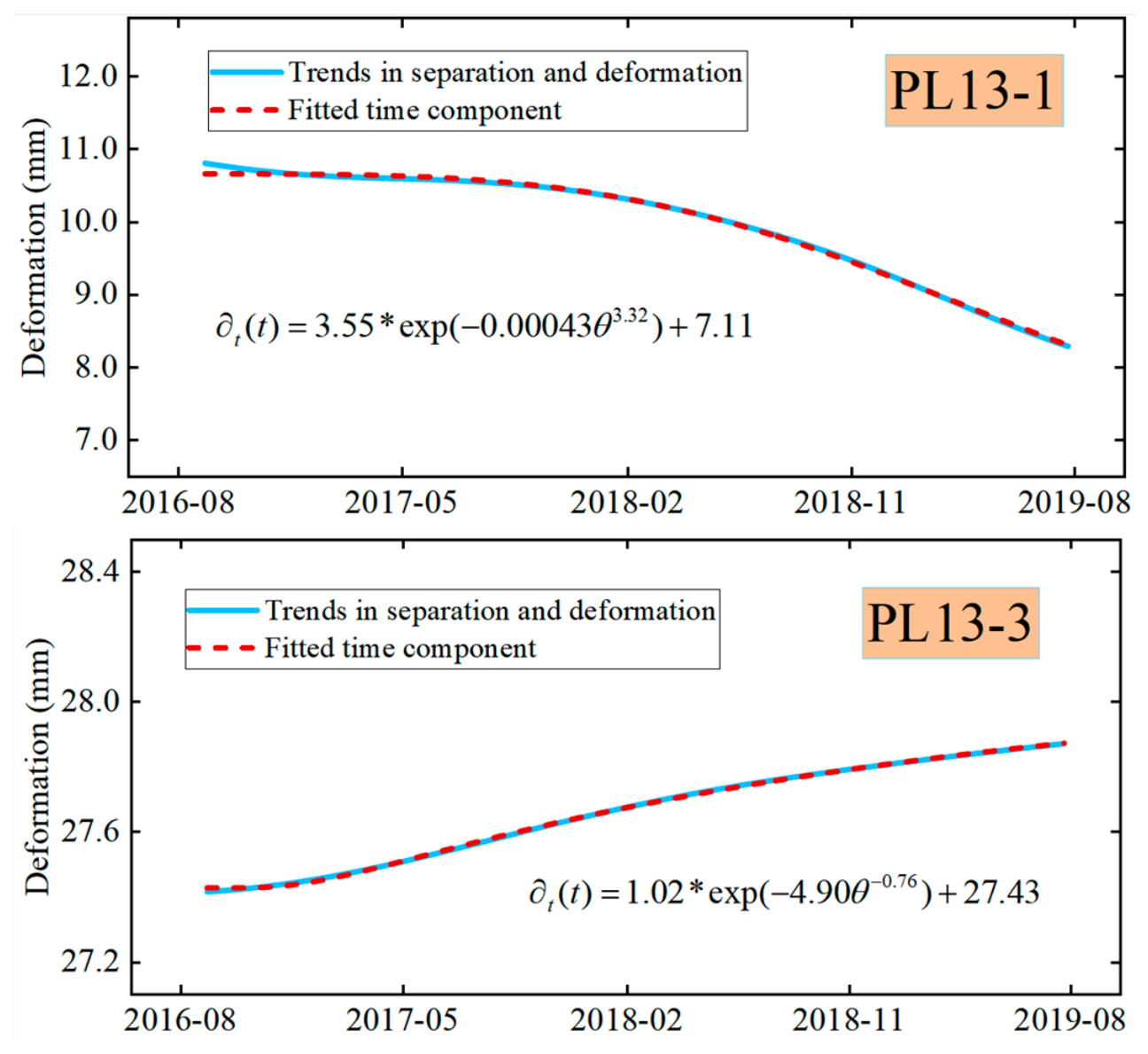
The extracted aging trend was then fitted using a composite exponential function to establish the aging component model. The fitted aging components of the radial displacements for PL13-1 and PL13-3 are presented in Figure 10, showing close agreement with the separated trend deformations and demonstrating good fitting performance.

3.2.2. Temperature Component Construction

In the present case, the reservoir water level exhibits substantial fluctuations, making it possible to isolate the temperature-induced deformation (i.e., the relative displacement caused solely by variations in dam temperature) from the periodic deformation component under the equal-water-level condition. Two observations are considered to satisfy this condition when the difference between their measured water levels is less than 0.02 m. Temperature-induced deformation is then obtained from pairs of observations with identical water levels extracted from the periodic deformation series. To reduce the influence of measurement errors, only displacement pairs associated with relatively large temperature differences under the same water-level condition are retained. The extracted temperature-induced deformation is subsequently fitted using conventional formulations, including linear combinations of moving-average air temperatures and seasonal harmonic functions, as well as the beta-distribution-based weighting scheme proposed in this study, thereby establishing the mathematical expression of the temperature component.

Instead of being purely empirical, the shape parameters (α, β) of the beta distribution mathematically map to the physical properties of the thermal impulse response P(t): α predominantly dictates the initial delay and the time required to reach the peak thermal response, which physically reflects the heat-transfer path length, such as the depth of the measurement point from the concrete surface. β governs the long-tail attenuation rate of the curve, which is related to the thermal inertia and thermal diffusivity of the concrete material. The parameter m acts as an amplitude scaling/shifting factor to convert the normalized probability density output into the actual physical magnitude of temperature or deformation. Therefore, the beta-distribution parameters provide a physically interpretable representation of the varied heat conduction processes at different spatial locations, as shown in Figure 2 and Figure 11.

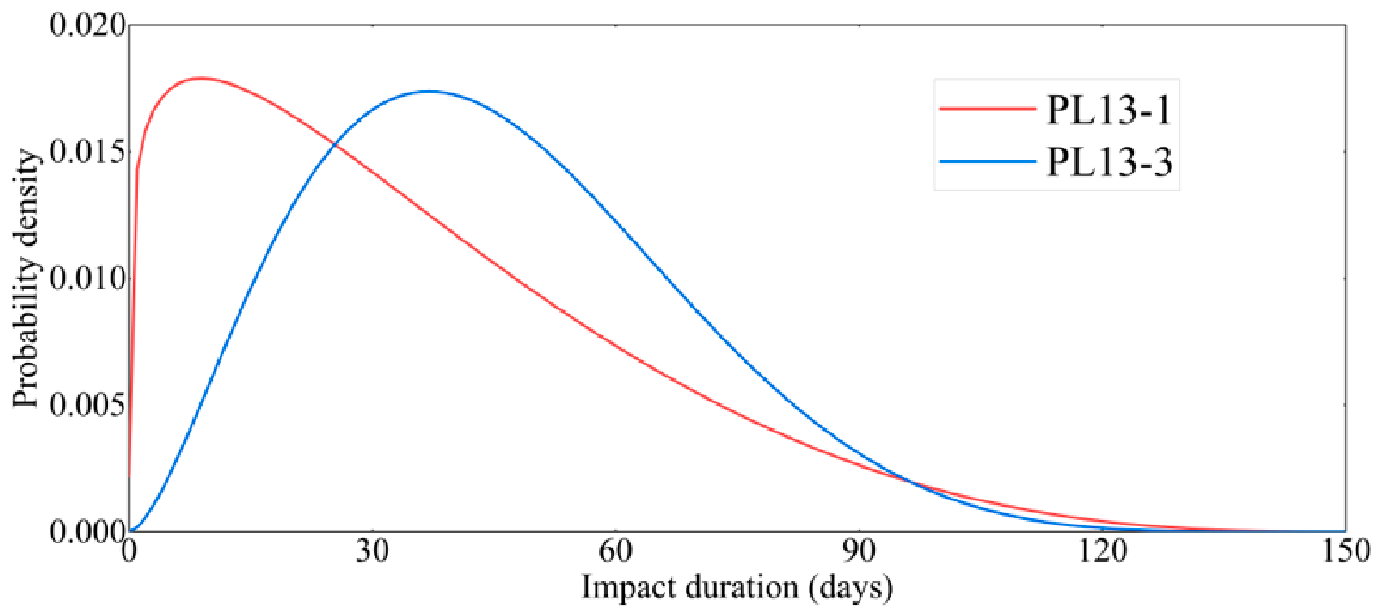
The extracted temperature-induced deformation was modeled using Equation (19), where the beta impact function B(t) was introduced to characterize the thermal lag effect. The optimal parameter set (α, β, and m) was derived by minimizing the objective function defined in Equation (20). Substituting these optimized parameters into the mathematical framework yields the specific beta impact functions B(t). The resulting parameters for each monitoring point are detailed in

Table 1. Beta parameters of monitoring points.

	Monitoring Points	PL13-1	PL13-3
Parameters
α		1.170	2.651
β		3.699	6.043
m		−1.010	−0.575

, and the corresponding beta impact function curves are illustrated in Figure 11.

The results (listed in

Table 2. Number of days in the affected period corresponding to the cumulative weight of each monitoring point.

	Monitoring Points	PL13-1	PL13-3
Cumulative Weight
30%		18	32
50%		30	43
70%		47	56
90%		75	76
100%		131	126

and

Table 3. Cumulative weight of deformation corresponding to early-stage temperatures.

	Monitoring Points	PL13-1	PL13-3
Time (Days)
3		0.044	0.001
6		0.095	0.007
10		0.167	0.025
15		0.255	0.064
30		0.493	0.270
60		0.813	0.746
120		0.997	0.999

) indicate that the duration of the ambient-temperature influence on deformation ranges from 126 to 131 days for all vertical monitoring points. This provides direct data validation for the predefined 150-day window. The cumulative weight already reached 0.997 at 120 days, as shown in Table 3, and approached 1.0 within 126–131 days. Therefore, selecting 150 days as the upper limit sufficiently covers the significant temperature influence while avoiding unnecessary extension of the historical window with negligible weighting. This choice represents a reasonable balance between theoretical completeness and computational efficiency. Along the arch direction, the lag effect showed no significant variation among different monitoring locations. For example, the number of days corresponding to a cumulative weight of 50% at the crest point PL13-1 ranged from 30 to 33 days, with differences not exceeding 3 days. Similar cumulative weights were observed for comparable influence durations; for instance, the cumulative weight associated with a 30-day period was approximately 0.493, indicating nearly identical lag characteristics.

In contrast, along the elevation direction, the lag effect at the crest was noticeably weaker than that at mid-height locations. For the mid-height point PL13-3 on the crown cantilever, the days corresponding to cumulative weights of 30%, 50%, and 70% were 32, 43, and 56 days, respectively, all exceeding those of the crest point. Moreover, for an influence duration of 30 days, the cumulative weight at PL13-3 was 0.270, substantially lower than that at the crest, further confirming the stronger lag effect in the central region of the dam. Comparison of the days corresponding to cumulative weights of 90% and 100% revealed only minor differences between the two monitoring points, suggesting that once the cumulative weight exceeds 70%, the contribution of ambient temperature to temperature-induced deformation becomes relatively small, and the influence of temperature fluctuations differs little among monitoring locations.

3.2.3. Water Pressure Component Construction

At the JP Hydropower Station, the upstream reservoir water level exhibits substantial fluctuations, whereas the downstream water level remains relatively stable with both small depth and limited variation. Therefore, only the influence of the upstream water level on deformation was considered when constructing the hydraulic component model. Given the considerable upstream water depth, the water-level variable was normalized to avoid coefficient scaling imbalance. The minimum and maximum water levels were taken as 1800.00 m and 1882.60 m, respectively, and the normalization scheme was defined by Equation (26). The coefficients of the water-level factors in the SMT-based monitoring models for each monitoring point are listed in

Table 4. Water level factor coefficients of monitoring models at each point based on decoupled modeling.

Model	Monitoring Points	h	h2	h3	h4	a0
SMT-S	PL13-1	15.762	8.197	18.998	−1.622	−21.234
	PL13-3	−19.149	19.346	14.672	0.783	−1.890
SMT-T	PL13-1	17.825	−4.103	25.699	−1.615	−2.938
	PL13-3	−8.618	22.294	11.435	−12.243	9.273
SMT-β	PL13-1	15.099	3.655	19.072	0.370	−1.845
	PL13-3	−7.743	21.605	9.874	−4.915	4.447

Note: SMT-S, SMT-T, and SMT-β are SMT-based models constructed using seasonal harmonic functions, moving-average air temperatures, and the proposed beta-distribution scheme as their respective temperature components.

.

3.3. Comparative Analysis

The study used radial displacement data from 2 September 2016 to 23 July 2019 to establish the monitoring models, and data from 24 July to 23 October 2019 to validate their predictive performance. This paper used the coefficient of determination (R²), root mean square error (RMSE), mean absolute error (MAE), mean absolute percentage error (MAPE), and overfitting coefficient (OC) as evaluation metrics for each model. The formula for calculating the overfitting coefficient (OC) and its significance is as follows:

$$OC={\displaystyle \frac{1}{3}}({\displaystyle \frac{RMS{E}_P}{RMS{E}_F}}+{\displaystyle \frac{MA{E}_P}{MA{E}_F}}+{\displaystyle \frac{MAP{E}_P}{MAP{E}_F}})$$

(29)

where OC is the overfitting coefficient of the monitoring model; the subscripts P and F are the model prediction segment and model fitting segment, respectively.

OC quantitatively reflects the degree of overfitting by comparing the model performance in the prediction segment with that in the fitting segment. When OC > 1, the prediction error is higher than the fitting error, indicating that the model exhibits overfitting; a larger OC indicates a greater degree of overfitting. Conversely, when OC < 1, the prediction error is lower than the fitting error, indicating no apparent overfitting and better model performance.

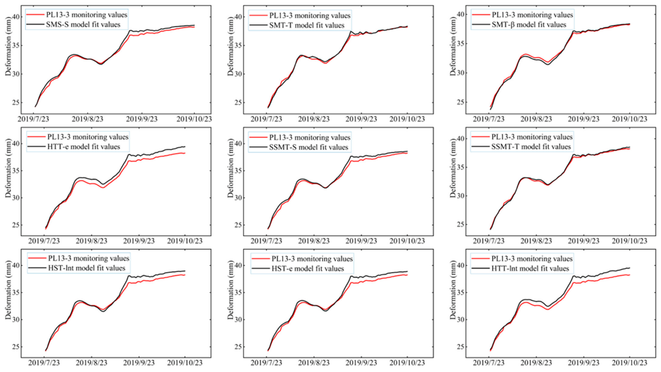
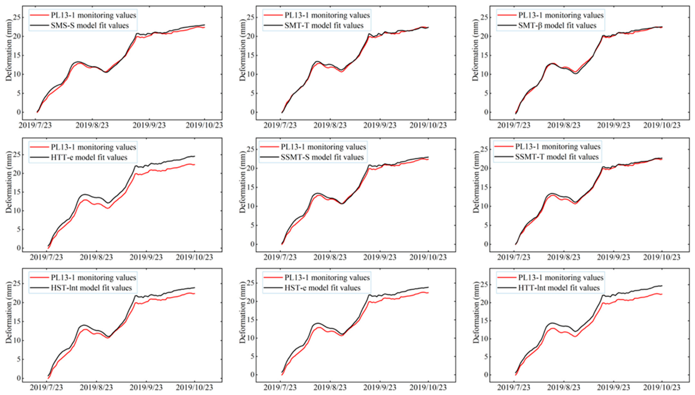
The prediction results of each model are shown in

Table 5. Evaluation metrics of the PL13-1 radial displacement monitoring model.

Monitoring Model	Fitting Segment Indicators				Prediction Segment Indicators			Overfitting Coefficient	False Alarm Rate
	R2	RMSE	MAE	MAPE	RMSE	MAE	MAPE	OC	FAR
		(mm)	(mm)	(%)	(mm)	(mm)	(%)
SMT-S	0.998	0.668	0.537	6.31	0.560	0.487	7.40	1.02	0%
SMT-T	0.996	0.963	0.777	14.79	0.379	0.297	6.34	0.36	0%
SMT-β	0.996	0.896	0.755	13.03	0.318	0.266	4.53	0.48	0%
HST-lnt	0.998	0.594	0.476	5.10	1.258	1.175	24.24	3.11	60%
HST-e	0.998	0.596	0.477	5.15	1.256	1.183	24.90	3.14	60%
HTT-lnt	0.998	0.608	0.505	8.44	1.694	1.631	24.65	2.98	77%
HTT-e	0.998	0.594	0.494	8.53	1.664	1.611	25.09	3.00	83%
SSMT-S	0.998	0.655	0.527	6.66	0.611	0.538	10.41	1.17	0%
SSMT-T	0.996	0.927	0.761	13.69	0.425	0.369	4.79	0.43	0%

and

Table 6. Evaluation metrics of the PL13-3 radial displacement monitoring model.

Monitoring Model	Fitting Segment Indicators				Prediction Segment Indicators			Overfitting Coefficient	False Alarm Rate
	R2	RMSE	MAE	MAPE	RMSE	MAE	MAPE	OC	FAR
		(mm)	(mm)	(%)	(mm)	(mm)	(%)
SMT-S	0.999	0.425	0.354	1.42	0.407	0.348	1.02	0.89	0%
SMT-T	0.996	0.726	0.548	2.53	0.230	0.174	0.54	0.28	0%
SMT-β	0.997	0.653	0.506	2.38	0.262	0.227	0.70	0.38	0%
HST-lnt	0.999	0.330	0.266	1.17	0.631	0.537	1.53	1.75	43%
HST-e	0.999	0.330	0.268	1.17	0.601	0.517	1.48	1.67	44%
HTT-lnt	0.997	0.591	0.459	1.94	0.817	0.751	2.14	1.37	4%
HTT-e	0.997	0.574	0.453	1.92	0.788	0.740	2.13	1.37	2%
SSMT-S	0.999	0.419	0.343	1.38	0.456	0.397	1.17	1.03	1%
SSMT-T	0.996	0.710	0.535	2.48	0.180	0.147	0.44	0.23	0%

, and the comparison between the observed values at the monitoring points with the predicted values is shown in Figure 12 and Figure 13. The comparative analysis is as follows:

(1) Model accuracy: the traditional statistical models (HTT and HST) exhibit higher fitting accuracy than the separated modeling approach (SMT). Taking the PL13-1 monitoring point as an example, the HST-lnt model achieved the best fitting metrics (RMSE = 0.594 mm, R² = 0.998), whereas the SMT-T model showed relatively poorer fit (RMSE = 0.963 mm). However, in terms of predictive accuracy, the SMT models outperformed the traditional models significantly. The SMT-β model exhibited minimal predictive deviation (RMSE = 0.318 mm), whereas the HST-lnt model showed considerably larger prediction errors (RMSE = 1.631 mm). These results indicate that while traditional statistical models can closely fit the radial displacement monitoring data with small fitting bias, their predictive performance is substantially lower than that of SMT-based monitoring models. The SMT models, although slightly less accurate in fitting during model construction, achieved much higher predictive accuracy, resulting in significantly smaller prediction deviations compared to traditional models.

It is noteworthy that the accuracy improvement of the proposed model over traditional models was larger at PL13-1 (Table 5) than at PL13-3 (Table 6). This difference is primarily attributed to the depth-dependent attenuation of thermal variations within the concrete. PL13-1, located near the crest, is more strongly affected by high-frequency transient temperature fluctuations (e.g., daily weather variations), which are difficult to fully capture using traditional harmonic models. Conversely, at the deeper PL13-3 point, the thermal inertia of the massive concrete effectively attenuates high-frequency variations, leaving predominantly smooth low-frequency seasonal changes. Since traditional harmonic models can reasonably represent these low-frequency seasonal effects, the relative improvement provided by the proposed framework naturally decreases at greater depths.

Furthermore, although the SMT-β framework incorporates signal decomposition and parameter optimization, these additional computations are mainly required during model establishment or updating. Once the model parameters are determined, the computational cost of routine prediction is very low and is not significantly different from that of traditional models. Given that the monitoring data are collected once per day, the proposed framework is computationally feasible for routine structural health monitoring of the dam.

(2) Overfitting and false alarm rate (FAR): traditional statistical models suffer from serious overfitting (overfitting coefficient (OC > 1.2)), leading to high false alarm rates. In contrast, the separated modeling technique effectively mitigates overfitting, keeping most models within the no-overfitting (OC < 1.0) or low-overfitting (1.0 < OC < 1.2) range. For instance, the HST and HTT series models exhibited (OC) values mostly between 2.98 and 3.14, with false alarm rates reaching 60–83%. Conversely, the SMT models significantly reduced overfitting (OC < 1.2); specifically, the (OC) values for SMT-T, SMT-S, and SMT-β were 0.36, 1.02, and 0.48, respectively, with all corresponding false alarm rates at 0%.

Although traditional statistical models achieve higher fitting accuracy, they do so through mathematical compensation among highly correlated variables, leading to severe overfitting. Because the SMT framework physically decouples these mechanisms prior to modeling, it prevents this mutual compensation. Consequently, while SMT yields slightly lower fitting metrics during the training phase, its components remain physically interpretable, resulting in significantly superior predictive accuracy and generalization on unseen data.

4. Conclusions

(1) This study overcomes the limitations of traditional models that rely on direct multi-factor regression by combining signal decomposition algorithms with controlled environmental conditions (constant water level or temperature), enabling independent decoupling and the modeling of time-dependent, hydraulic, and thermal components. To address large water-level fluctuations and complex heat exchange boundaries, the transient heat conduction equation was used to derive the lagged influence weights of air temperature on the dam body, and a beta distribution was innovatively introduced to construct the temperature component model. This model accurately quantifies the asymmetric attenuation of thermal deformation and effectively addresses the limitations of traditional harmonic functions under extreme climate and water-level fluctuations.

(2) Comparative analysis indicates that traditional models suffer from severe multicollinearity among factors, leading to pronounced overfitting and high false alarm rates. The proposed SMT-β model, through its separated modeling strategy, eliminates the mathematical compensation effects between components, significantly reducing overfitting and demonstrating superior generalization ability and stability in deformation prediction.

(3) Due to limitations in monitoring point density and the study period, the current modeling of the JP double-curvature arch dam does not fully capture the spatiotemporal evolution of the dam and foundation temperature fields. Future research will expand the spatial modeling scope, investigate the coupled effects of dynamic reservoir water-level variations on dam temperature boundary conditions, and explore the application of this model to other hydraulic structures such as gated dams and protective levees, aiming to develop an intelligent deformation monitoring system encompassing the entire hydropower hub.

References

1. Tonini, D. Observed behavior of several Italian arch dams. J. Power Div. 1956, 82, 1134-1. [Google Scholar] [CrossRef] [Scilit]
2. Li, F.; Wang, Z.; Liu, G.; Fu, C.; Wang, J. Hydrostatic seasonal state model for monitoring data analysis of concrete dams. Struct. Infrastruct. Eng. 2015, 11, 1616–1631. [Google Scholar] [CrossRef] [Scilit]
3. Shen, D.B.; Huang, H.B.; Wang, D.; Hu, M.X. Research on new statistical model of horizontal displacement monitoring in gravity dam. Water Resour. Power 2012, 30, 81–84. [Google Scholar]
4. Wei, B.; Xiong, W.; Li, H.; Peng, S.; Xu, Z. Dam deformation forecasting of leapfrog combined model merging residual errors of chaos. Geomat. Inf. Sci. Wuhan Univ. 2016, 41, 1272–1278. [Google Scholar]
5. Zhang, Y.J.; Zheng, D.J.; Zheng, Z.T. Deformation prediction model and application of concrete dams based on optimized fruit fly optimization algorithm and statistical model. Water Resour. Power 2019, 37, 91–94. (In Chinese) [Google Scholar]
6. Gu, X.; Shen, Z. A deformation monitoring model for concrete dams based on PSO-ASIN. In Proceedings of the 2010 3rd International Conference on Biomedical Engineering and Informatics, Yantai, China, 16–18 October 2010; IEEE: Piscataway, NJ, USA, 2010; Volume 7, pp. 3012–3015. [Google Scholar]
7. Xiong, F.; Wei, B.; Xu, F.; Zhou, L. Deterministic combination prediction model of concrete arch dam displacement based on residual correction. Structures 2022, 44, 1011–1024. [Google Scholar] [CrossRef] [Scilit]
8. Gu, C.; Fu, X.; Shao, C.; Shi, Z.; Su, H. Application of spatiotemporal hybrid model of deformation in safety monitoring of high arch dams: A case study. Int. J. Environ. Res. Public Health 2020, 17, 319. [Google Scholar] [CrossRef] [Scilit] [PubMed]
9. Yang, G.; Gu, H.; Chen, X.; Zhao, K.; Qiao, D.; Chen, X. Hybrid hydraulic-seasonal-time model for predicting the deformation behaviour of high concrete dams during the operational period. Struct. Control Health Monit. 2021, 28, e2685. [Google Scholar] [CrossRef] [Scilit]
10. Song, L.; Hu, Y. Data–Physics-Driven Multi-Point Hybrid Deformation Monitoring Model Based on Bayesian Optimization Algorithm–Light Gradient-Boosting Machine. Water 2025, 17, 2926. [Google Scholar] [CrossRef] [Scilit]
11. Qi, Y.; Su, H.; Yao, K. Dam deformation analysis model based on characteristic decomposition screening of coupling timeseries. Hydroelectr. Eng. 2023, 42, 56–68. [Google Scholar]
12. Wu, M.; Su, H.-Z.; Yang, L. Combined modeling method of PCA-WOA-LSSVM for deformation prediction model of concrete dam. Hydro Energy Sci. 2022, 40, 111–114. [Google Scholar]
13. Li, S.P.; Zhang, B.; Liu, Z.Q. A new prediction model of dam deformation and successful application. Buildings 2025, 15, 818. [Google Scholar] [CrossRef] [Scilit]
14. Zhang, Y.; Zhong, W.; Li, Y.; Wen, L. A deep learning prediction model of DenseNet-LSTM for concrete gravity dam deformation based on feature selection. Eng. Struct. 2023, 295, 116827. [Google Scholar] [CrossRef] [Scilit]
15. Madiniyeti, J.; Chao, Y.; Li, T.; Qi, H.; Wang, F. Concrete Dam Deformation Prediction Model Research Based on SSA–LSTM. Appl. Sci. 2023, 13, 7375. [Google Scholar] [CrossRef] [Scilit]
16. Liu, Y.; Zheng, D.; Georgakis, C.; Kabel, T.; Cao, E.; Wu, X.; Ma, J. Deformation Analysis of an Ultra-High Arch Dam under Different Water Level Conditions Based on Optimized Dynamic Panel Clustering. Appl. Sci. 2022, 12, 481. [Google Scholar] [CrossRef] [Scilit]
17. Wang, R.J.; Bao, T.F.; Li, Y.T.; Song, B.G.; Xiang, Z.Y. Combined prediction model of dam deformation based on multi-factor fusion and stacking ensemble learning. J. Hydrostatic Eng. 2023, 54, 497–506. [Google Scholar]
18. Mata, J.; Tavares De Castro, A.; Sá Da Costa, J. Constructing statistical models for arch dam deformation. Struct. Control Health Monit. 2014, 21, 423–437. [Google Scholar] [CrossRef] [Scilit]
19. Penot, I.; Daumas, B.; Fabre, J.P. Monitoring behavior [dam behavior monitoring]. Int. Water Power Dam Constr. 2005, 57, 24–27. [Google Scholar]
20. Tatin, M.; Briffaut, M.; Dufour, F.; Simon, A.; Fabre, J.P. Thermal displacements of concrete dams: Accounting for water temperature in statistical models. Eng. Struct. 2015, 91, 26–39. [Google Scholar] [CrossRef] [Scilit]
21. Tatin, M.; Briffaut, M.; Dufour, F.; Simon, A.; Fabre, J.P. Statistical modelling of thermal displacements for concrete dams: Influence of water temperature profile and dam thickness profile. Eng. Struct. 2018, 165, 63–75. [Google Scholar] [CrossRef] [Scilit]
22. Li, B.; Yang, J.; Hu, D. Dam monitoring data analysis methods: A literature review. Struct. Control Health Monit. 2019, 27, e2501. [Google Scholar] [CrossRef] [Scilit]
23. Ren, Q.B.; Li, M.C.; Song, L.G.; Liu, H. An optimized combination prediction model for concrete dam deformation considering quantitative evaluation and hysteresis correction. Adv. Eng. Inform. 2020, 46, 101154. [Google Scholar] [CrossRef] [Scilit]
24. Kang, F.; Li, J. Displacement Model for Concrete Dam Safety Monitoring via Gaussian Process Regression Considering Extreme Air Temperature. Struct. Eng. 2020, 146, 05019001. [Google Scholar] [CrossRef] [Scilit]
25. Lu, T.; Gu, C.; Yuan, D.; Zhang, K.; Shao, C. Deep learning model for displacement monitoring of super high arch dams based on measured temperature data. Measurement 2023, 222, 113579. [Google Scholar] [CrossRef] [Scilit]
26. Pan, J.; Liu, W.; Wang, J.; Jin, F.; Chi, F. A novel reconstruction method of temperature field for thermomechanical stress analysis of arch dams. Measurement 2022, 188, 110585. [Google Scholar] [CrossRef] [Scilit]
27. Xu, B.; Yao, Y.; Wang, X.; Sun, L.; Ou, B.; Zhang, Y. A Multi-Input Multi-Output Considering Correlation and Hysteresis Prediction Method for Gravity Dam Displacement with Interpretative Functions. Appl. Sci. 2025, 15, 7096. [Google Scholar] [CrossRef] [Scilit]
28. Léger, P.; Leclerc, M. Hydrostatic, temperature, time-displacement model for concrete dams. J. Eng. Mech. 2007, 133, 267–277. [Google Scholar] [CrossRef] [Scilit]
29. Lin, C.; Zou, Y.; Lai, X.; Wang, X.; Su, Y. Variation Trend Prediction of Dam Displacement in the Short-Term Using a Hybrid Model Based on Clustering Methods. Appl. Sci. 2023, 13, 10827. [Google Scholar] [CrossRef] [Scilit]
30. Xiong, C.; Shang, Z.; Wang, M.; Lian, S. Dynamic Monitoring of a Bridge from GNSS-RTK Sensor Using an Improved Hybrid Denoising Method. Sensors 2025, 25, 3723. [Google Scholar] [CrossRef] [Scilit] [PubMed]
31. Bofang, Z. Thermal Stresses and Temperature Control of Mass Concrete; Butterworth-Heinemann: Oxford, UK, 2013. [Google Scholar]
32. Guo, X.; Baroth, J.; Dias, D.; Simon, A. An analytical model for the monitoring of pore water pressure inside embankment dams. Eng. Struct. 2018, 160, 356–365. [Google Scholar] [CrossRef] [Scilit]
33. Wang, L. Deformation Monitoring Model of Xin’anjiang Gravity Dam Based on Support Vector Machine. Master’s Thesis, Kunming University of Science and Technology, Kunming, China, 2016. (In Chinese) [Google Scholar]
34. China Power Construction Group Co., Ltd. A Documentary Account of the Construction of the Jinping I Hydropower Station, Winner of the Zhan Tianyou Award. 2018. Available online: http://www.sasac.gov.cn/n2588025/n2588159/c9125452/content.html (accessed on 26 August 2026).
Figure 1. Typical beta distribution curve.
Applsci 16 08670 g001
Figure 2. Common forms of the P(t) function: (a) monitoring points close to the dam face; (b) monitoring points far from the dam face.
Applsci 16 08670 g002
Figure 3. Flowchart of the separate modeling technique based on equal water level conditions.
Applsci 16 08670 g003
Figure 4. Flowchart of the separate modeling technique based on isothermal conditions.
Applsci 16 08670 g004
Figure 5. Aerial view of the JP hydropower project [34].
Applsci 16 08670 g005
Figure 6. (a) Monitoring layout of thermometers on the dam body at dam section 13. (b) Monitoring layout along the plumb line of the JP arch dam.
Applsci 16 08670 g006
Figure 7. Time-series curves of the upstream and downstream water levels at the JP arch dam.
Applsci 16 08670 g007
Figure 8. Time-series plot of the daily average temperature in the JP hydropower station dam area.
Applsci 16 08670 g008
Figure 9. Time-dependent deformation extracted by the ICEEMDAN.
Applsci 16 08670 g009
Figure 10. Time-dependent component curve fitting.
Applsci 16 08670 g010
Figure 11. Probability density curves of the beta distribution of monitoring points.
Applsci 16 08670 g011
Figure 12. Comparison of the observed and predicted values of PL13-1.
Applsci 16 08670 g012
Figure 13. Comparison of the observed and predicted values of PL13-3.
Applsci 16 08670 g013