A Population-Calibrated MAP-Type Estimator for Induction Motor Equivalent-Circuit Parameters from Nameplate Data

Featured Application

A population-calibrated, MAP-type estimator of induction motor equivalent-circuit parameters from manufacturer catalog data alone, with measured accuracy and a measured validity range. It supplies the steady-state layer of a digital twin, energy auditing and model-based engineering where IEEE Std 112 testing is impractical.

Abstract

Identifying induction-motor equivalent-circuit parameters from nameplate data is challenging without the IEEE Std 112 no-load and locked-rotor tests. This study reformulates the task from constraint-based curve fitting to population-calibrated maximum-a-posteriori (MAP)-type estimation of seven steady-state parameters. Under an identical protocol, the best of fifteen metaheuristics reached 14.71% global error against 23.40% for the best analytical method; its residual structure motivates the central step: closed-form nameplate predictors, calibrated on a five-motor reference population, become Gaussian prior means whose cross-validated dispersions set the prior widths and the $\pm 3\sigma$ search bounds. Re-anchoring the loss priors to a per-machine constant-loss decomposition (MAP+) lowers the apparent error to 3.48%, and nested leave-one-out cross-validation, re-calibrating all statistical quantities per fold, gives a validated 4.27%. With algorithm, budget and seeds fixed, formulation outweighs optimizer choice. Withholding catalog quantities and predicting them back gives forty out-of-fit checks on ten machines: rated current within 0.96% and partial-load power factor within 2.65%, but the breakdown-torque ratio only within 9.04%, proving it an input rather than an output; locked-rotor errors confine the single-cage model to running operation. It offers a calibrated, validity-bounded basis for the steady-state layer of digital twins and energy auditing, not a general-purpose estimator.

1. Introduction

Three-phase induction motors (IMs) are the dominant electromechanical energy conversion devices in modern industry because of their robustness, reliability, low maintenance requirements, and cost-effectiveness. They account for the majority of industrial electricity consumption and play a fundamental role in manufacturing, transportation, mining, and energy production. Consequently, accurate mathematical models of induction motors are essential for performance prediction, vector control, fault diagnosis, condition monitoring, energy-efficiency assessment, and the development of digital twins [1].

Among the available modeling approaches, the steady-state equivalent circuit remains the most widely adopted because it provides an appropriate balance between physical interpretability and computational efficiency. The predictive capability of this model, however, depends directly on the accurate identification of its electrical parameters. Traditionally, these parameters are obtained through no-load and locked-rotor tests standardized in IEEE Std 112 [2]. Although these procedures provide reliable parameter estimates, they require specialized laboratory equipment, controlled operating conditions, and temporary removal of the machine from service. Consequently, they are often impractical for motors already installed in industrial facilities, motivating the search for non-intrusive identification techniques based exclusively on manufacturer-provided information [3].

Over the last two decades, considerable research has focused on estimating equivalent-circuit parameters from manufacturer catalog or nameplate data. Analytical methods have attracted particular attention because they provide fast and deterministic solutions without requiring iterative optimization. Several studies have demonstrated that properly formulated analytical approaches can achieve high statistical robustness across large populations of industrial motors while avoiding some of the convergence difficulties associated with recursive estimation procedures [4,5,6]. Other investigations have shown that incorporating variable rotor parameters or improved loss segregation significantly enhances the prediction of efficiency under steady-state operating conditions [7,8]. Sensitivity analyses have further revealed that certain parameters, particularly stator resistance, exert limited influence on the electrical performance variables, making the identification problem poorly conditioned unless additional physical constraints are introduced [9]. Review studies accordingly conclude that combining complementary estimation strategies provides greater robustness than relying on a single analytical formulation [10], a conclusion reinforced by the most recent assessment of nine such methods for nonintrusive loss estimation [11].

The highly nonlinear nature of the induction motor equivalent circuit has also motivated the adoption of metaheuristic optimization algorithms. Unlike deterministic analytical methods, metaheuristics can simultaneously optimize multiple strongly coupled parameters without requiring explicit gradient information. Evolutionary algorithms, swarm intelligence, differential evolution, and physics-inspired optimization techniques have all demonstrated promising performance for induction motor parameter identification. Representative examples include bacterial foraging optimization, Improved Moth Flame Optimization (IMFO), Sparse Grid Optimization, and Mean-Variance Optimization [12,13,14,15], and the stream of algorithmic variants remains active, as illustrated by a recent enhanced grey wolf optimizer applied to commercial machines [16]. Across this literature, however, reported gains are pursued almost exclusively through new search mechanisms operating on essentially unchanged problem formulations, and the performance of every such algorithm remains highly dependent on the definition of search-space boundaries, objective functions, and engineering constraints.

More recently, advances in Industry 4.0 have stimulated the development of data-driven approaches for induction motor modeling. Machine learning techniques, adaptive neuro-fuzzy inference systems, and surrogate models have been proposed to support real-time monitoring, predictive maintenance, and digital twin applications [17]. Likewise, recent reviews emphasize that while finite-element analysis continues to represent the reference standard for electromagnetic accuracy, data-driven surrogate models are becoming increasingly important for reducing computational cost in large-scale optimization and multiphysics simulations [1,18]. These developments demonstrate the growing importance of computational methodologies capable of extracting reliable machine models from limited experimental information.

A common trait runs through all three families of methods: the estimation is treated as deterministic curve fitting, and whatever engineering knowledge enters the problem does so as hard information—fixed per-unit bounds, prescribed reactance ratios, or heuristic relationships imposed as exact constraints [19]. This treatment has two consequences. First, the placement of bounds and relationships is rarely justified beyond expert experience, yet the final estimates can depend on it strongly, which limits reproducibility across motor ratings and manufacturers. Second, hard constraints offer no mechanism for weighing prior knowledge against the observed data: a bound either binds, or it does not. The theory of inverse problems has long offered the appropriate middle ground—casting prior knowledge as a probability distribution and the estimate as a maximum a posteriori (MAP) solution [20]. Furthermore, the empirical Bayes paradigm supplies the calibration route when the prior moments can be measured on a reference population rather than postulated [21]. To the best of the authors’ knowledge, this formulation has not been applied to nameplate-based induction motor parameter identification.

The absence of a statistical treatment matters because the nameplate identification problem is only partially identifiable. The catalog data constrain some parameters tightly, but they are nearly silent along specific directions of the parameter space: the stator resistance exerts little influence on the steady-state variables [9], and the core-loss resistance and the rotational losses act as almost interchangeable constant-loss mechanisms. Along these directions, many parameter combinations reproduce the nameplate equally well, and an unregularized optimizer selects among them arbitrarily. In addition, because relatively few studies evaluate multiple optimization strategies under identical physical assumptions, objective functions, and search spaces, it is generally impossible to distinguish improvements produced by the optimization algorithm from those produced by the engineering constraints embedded in the formulation.

This work addresses these gaps through a two-stage methodology. First, it establishes a physically constrained optimization framework in which fifteen representative metaheuristic optimizers operate under identical modeling assumptions, impedance-scaled search spaces, IEEE Std 112 leakage-reactance constraints, and independent treatment of core and rotational losses. This controlled benchmark is not intended to rank optimization algorithms, but to isolate the influence of the estimation formulation under identical optimization conditions. The residual error structure observed in this benchmark then motivates the second stage: a MAP-type estimator, calibrated in the empirical-Bayes sense, in which closed-form nameplate predictors become Gaussian prior means, their cross-validated dispersions define prior uncertainties, and both the search bounds and the regularization strength are derived from measured quantities rather than expert tuning. The methodology is finally validated on benchmark motors, commercial machines, and extended-range catalog datasets spanning 7.5 to 115 kW. The scope of the claim is deliberately bounded: calibrated on five reference machines, this work does not establish a general-purpose estimator, but demonstrates that nameplate-based identification can be placed on a measured statistical footing whose accuracy and validity range are both quantified—which is the prerequisite for the larger, multi-manufacturer calibration that genuine generalization would require.

The primary contributions of this paper are as follows.

• Unified Physically Constrained Identification Framework. A reproducible optimization environment—the Polymorphic Optimization Engine—in which fifteen metaheuristic algorithms spanning the principal families of modern stochastic optimization are benchmarked under identical objective functions, constraints, and search spaces, allowing the influence of the algorithm to be separated from that of the formulation.
• Closed-Form Nameplate Predictors. Six parameter predictors (plus one imposed design-class ratio, $X_1/X_2=0.68$) derived from approximate circuit arguments, each governed by a single dimensionless coefficient calibrated on the reference motor population, providing a measured, parameter-by-parameter map of how much information the nameplate actually contains.
• Population-Calibrated MAP-Type Estimator.A maximum a posteriori formulation in which the predictors become Gaussian prior means, their leave-one-out cross-validated relative root-mean-square error (RMSE) becomes the prior standard deviation ($\sigma$), and the search box becomes the $\pm 3\sigma$ interval of the prior. Its accuracy is certified by nested cross-validation rather than by resubstitution. This construction directly resolves the stator-resistance insensitivity and the core/rotational loss collinearity. A refinement of this estimator, denoted MAP+ hereafter, re-anchors the two loss priors to a per-machine constant-loss decomposition of the catalog efficiency points; it is the configuration adopted for the validation experiments of Section 4.5, Section 4.6, Section 4.7 and Section 4.8.
• Evidence that Formulation Outweighs Algorithm Selection. Demonstration that upgrading the physical formulation to MAP+ produces substantially larger accuracy gains than changing the optimization algorithm under the experimental conditions considered, indicating that improvements in the information structure have a greater impact on estimation accuracy than further refinement of the search strategy. Over thirty independent runs per motor–algorithm pair, a Friedman test detects significant differences among six representative algorithms on all five reference motors under the constraint-based formulation, and none under MAP+ (pooled $p=0.730$). The formulation, therefore, does not merely outweigh the choice of optimizer: it removes that choice as a source of variation.

The remainder of this paper is organized as follows. Section 2 reviews related work on analytical, metaheuristic, and statistical estimation. Section 3 presents the physically constrained optimization framework, the nameplate predictors and their cross-validation, and the empirical-Bayes MAP formulation. Section 4 reports the benchmark results, the ablation isolating the contribution of each ingredient of the MAP estimator, and the validation on commercial and simulated machines. Section 5 discusses the findings, Section 6 the limitations and future work, and Section 7 concludes.

2. Related Work

2.1. Analytical Estimation from Manufacturer Data

Analytical formulations dominate the early literature because they resolve the equivalent circuit in closed form from a handful of catalog quantities. Representative methods differ mainly in which data they consume and which simplifications they accept: fixed loss distributions, prescribed reactance ratios, or iterative refinements of an initial algebraic solution [4,5,6,8]. Variable rotor parameters and improved loss segregation extend their validity toward partial-load efficiency prediction [7]. The comparative assessment of Wengerkievicz et al. [10], whose five laboratory-characterized machines serve as the reference benchmark of the present work, found no analytical method uniformly superior: global parameter errors remained above 23% for even the best formulation, and the authors recommended combining complementary strategies. Their recent follow-up, which evaluates nine methods from the perspective of nonintrusive loss estimation, reaches a consistent conclusion [11]. Double-cage and multi-cage extensions estimate richer rotor models from the same data type, at the cost of more unknowns per observation [22,23].

2.2. Metaheuristic and Hybrid Estimation

Metaheuristics entered the field to escape the algebraic simplifications of analytical methods, and the catalog of applied algorithms now spans essentially every family of stochastic optimization: genetic algorithms with heuristic support relations [19], moth-flame and gravitational variants [12,13], sparse-grid and mean-variance formulations [14,15], two-stage particle swarm schemes applied to commercial machine populations [24], in-situ estimation from field measurements [25], and, most recently, an adaptively weighted grey wolf optimizer evaluated on eight commercial motors [16]. Three features recur across this literature. First, improvements are sought almost exclusively in the search mechanism, while the problem formulation—objective residuals, bounds, constraint treatment—changes little from study to study and is rarely justified beyond expert experience. Second, formulations frequently include auxiliary free variables, the operating slip among them, that improve the reported fit at the expense of physical consistency: a circuit that reproduces the torque triplet at a fictitious slip misplaces the entire torque–speed characteristic. Third, reported fitness values are not comparable across studies because they depend on the residual definition and on the ratio of unknowns to observations; near-zero fitness in exactly determined formulations signals interpolation, not accuracy.

Beyond parameter identification, surrogate-assisted and robust multi-objective formulations are well established in electrical-machine design, where radial-basis-function models stand in for expensive finite-element evaluations and manufacturing tolerances are carried explicitly through the optimization [26]. The cubic scaling of the surrogate fit that constrains the evaluation budget in those studies is the same effect that governs the two surrogate-assisted methods of the present benchmark, and it is quantified in Section 4.4. These observations motivate the controlled, single-formulation multi-algorithm benchmark of Section 3.3.

Although a broad spectrum of methodologies has been proposed to identify the equivalent-circuit parameters of the induction machine, a large fraction of them optimize almost exclusively against the torque behavior [27]—rated torque and the breakdown-torque ratio—while efficiency and power factor (PF) are relegated to secondary residuals or omitted altogether. This torque-centric formulation is problematic because the nameplate identification problem is only partially identifiable: multiple parameter sets can reproduce the prescribed torque triplet with near-zero residual and still be physically wrong when the same circuit is asked to predict efficiency, power factor, or the partial-load loss split [9]. In other words, an excellent torque fit is a necessary but by no means sufficient condition for a correct model. This over-fitting to torque—well illustrated by formulations that admit the operating slip as a free variable, thereby displacing the entire torque–speed characteristic—motivates the present work’s emphasis on jointly weighting mechanical and electrical indicators and on regularizing the weakly-observable directions through population-calibrated priors.

2.3. Statistical Treatment, Uncertainty, and Machine Learning

A separate line of work quantifies uncertainty in motor characterization, though almost exclusively on the measurement side: the tolerance and uncertainty structure of efficiency determination under IEC 60034-2-1 has been examined in detail [28,29], establishing that catalog quantities carry heterogeneous, known uncertainty levels. That knowledge, however, has not propagated into the estimation problem itself: parameter identification studies continue to treat catalog values as exact and prior knowledge as hard constraints. In the broader system-identification literature, the standard remedy for partially identifiable inverse problems is Bayesian regularization—casting prior knowledge as probability distributions and estimating by maximum a posteriori, which reduces to Tikhonov-type penalties under Gaussian assumptions [20]—with empirical Bayes supplying calibrated prior moments when a reference population is available [21]. Applications of this machinery to electrical machines exist for dynamic model learning, notably physics-informed neural networks that embed machine equations into data-driven models [30], and machine learning has been applied to online parameter tracking and condition monitoring [17]. To the best of the authors’ knowledge, no previous study formulates nameplate-based equivalent-circuit identification as a MAP problem with population-calibrated priors.

2.4. Benchmarks, Data, and Reproducibility

The field lacks a standardized benchmark. The five-motor dataset of Wengerkievicz et al. [10] is the closest to a common reference for single-cage identification, and commercial machine collections have begun to circulate: eight motors spanning 3 to 37 kW introduced with a two-stage particle swarm optimization (PSO) scheme [24] and reused in subsequent algorithm studies [16], and a two-hundred-motor population (22–90 kW) employed for multi-cage validation [23]. Open datasets oriented to efficiency monitoring and to design-parameter learning have also been published [31]. Reuse of these collections, however, requires some caution. Their documentation is primarily torque-oriented (partial-load efficiency and power-factor points are frequently not published), so they cannot exercise the loss-segregation capability that distinguishes full seven-parameter identification, which is why the present work validates on machines with complete catalog documentation instead. The data-consistency screening of Section 3.1 is a direct response to these observations.

3. Materials and Methods

3.1. Framework Overview and Experimental Datasets

This research develops a parameter identification methodology in two stages. The first stage is a physically constrained optimization framework in which heterogeneous metaheuristic algorithms estimate the seven steady-state equivalent-circuit parameters of an induction motor from manufacturer catalog data, under common engineering constraints. The second stage, motivated by the residual error structure observed in the first, replaces the deterministic constraint set with a statistical one: closed-form parameter predictors calibrated on a reference motor population become the means of Gaussian priors, and the estimation is reformulated as a maximum a posteriori problem. The first stage reproduces the constraint-based practice that dominates the literature [27] and serves as its controlled representative; the second quantifies exactly what the statistical treatment adds.

Nameplate-based estimation admits many mathematically valid solutions that do not correspond to physically realistic machines. The framework confronts this at two levels: impedance-scaled search spaces that exclude electromagnetically implausible regions and IEEE Std 112 leakage-reactance constraints, and in the second stage, priors that penalize departures from population-typical values in proportion to how well each parameter can be predicted from the nameplate alone.

Three complementary datasets support the evaluation. The first consists of five benchmark induction motors rated between 7.5 and 75 kW, taken from the study of Wengerkievicz et al. [10], whose laboratory-tested reference parameters permit direct error quantification and comparison with six analytical methods from the literature. The second comprises three commercial WEG W22 machines (15, 30, and 55 kW) for which there are no reference parameters [32]; their role is to verify that the framework reconstructs realistic operating characteristics from catalog information alone. The third consists of two catalog-style datasets published in [11] for machines rated 11 kW and 115 kW, whose performance values are computed from motor models rather than measured in a laboratory and which include the partial-load points; they extend the evaluation beyond the power range, voltage class, and line frequency of the calibration population, and no predictor coefficient was adjusted to accommodate them.

For all machines, the optimization is driven by the manufacturer catalog vector

$${\mathrm{D}}_{cat}=[P_{rated},V_{rated},f,p,n_{rated},I_{rated},T_{max}/T_{rated},{\eta }_{vec},{PF}_{vec}]$$

(1)

where $P_{rated}$, $V_{rated}$, f, p, $n_{rated}$, $I_{rated}$, and $T_{rated}$ denote rated power, voltage, supply frequency, pole number, speed, current, and torque (the frequency and pole number set the synchronous speed and slip), and ${\eta }_{vec}$ and ${PF}_{vec}$ collect the efficiency and power-factor values at 50%, 75%, and 100% load. The partial-load points carry the only information in the catalog capable of separating constant from load-dependent losses, and their inclusion proves essential for the identification of the loss parameters.

Before estimation, every dataset is screened for internal consistency using two identities that catalog data must satisfy: the rated torque must equal $P_{rated}/{\omega }_{rated}$, and the rated current must equal $P_{rated}/\left(\sqrt{3}{V}_{rated}PF\eta \right)$. The screening is inexpensive and consequential: a residual that cannot be driven below the catalog rounding level usually indicates an error in the source data rather than in the model. All machines used in this study satisfy both identities to three significant figures.

The software infrastructure was developed using a Human-in-the-Loop (HITL) workflow assisted by Large Language Models (LLMs). Domain experts defined the equivalent-circuit topology, the constraints, the admissible parameter ranges, the objective function, and the validation procedures; the language models served as implementation tools for code generation, algorithm integration, and debugging. Engineering expertise, therefore, remained responsible for every physical assumption and validation decision, artificial intelligence (AI) assistance compressed the implementation effort.

3.2. Steady-State Equivalent-Circuit Model

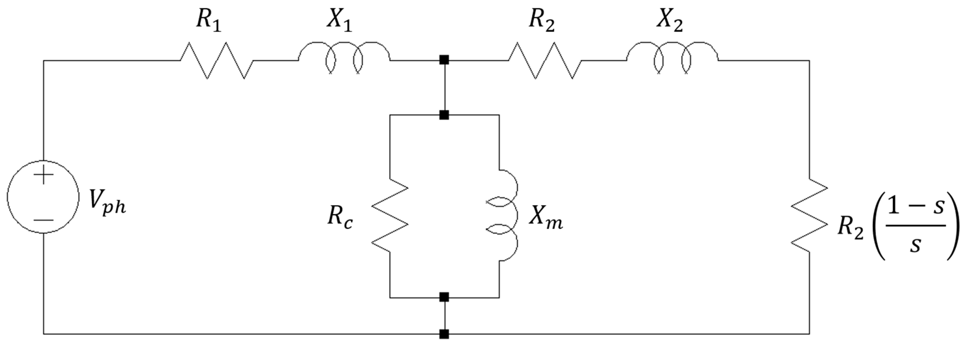
The machine is represented by the exact single-cage equivalent circuit shown in Figure 1 with the magnetizing reactance $X_m$ in parallel with a core-loss resistance $R_c$, and with the rotational losses $P_{rot}$ treated as a separate mechanical term rather than lumped into the magnetic branch. $R_1$ and $R_2$ are the stator and rotor resistances, while $X_1$ and $X_2$ represent the stator and rotor reactances.

At slip s, the branch impedances per phase are as follows:

$$Z_g={\displaystyle \frac{j{X}_m{R}_c}{R_c+j{X}_m}},Z_r={\displaystyle \frac{R_2}{s}}+j{X}_2,Z_{eq}=R_1+j{X}_1+{\displaystyle \frac{Z_g{Z}_r}{Z_g+Z_r}}$$

(2)

From which the stator current, power factor, and input power follow Equations (3)–(6)

$$I_1=V_{ph}/\left|Z_{eq}\right|$$

(3)

$$PF=\cos (\angle Z_{eq})$$

(4)

$$P_{in}=3V_{ph}{I}_{1}PF$$

(5)

$$V_{ph}=V_{rated}/\sqrt{3}$$

(6)

The electromagnetic torque ($T_{em}$) is evaluated through the Thevenin equivalent seen by the rotor branch when a phase voltage ($V_{ph}$) is applied, as shown in Equation (7).

$$T_{em}\left(s\right)={\displaystyle \frac{3V_{th}^2(R_2/s)}{{\omega }_s\left[{(R_{th}+R_2/s)}^2+{(X_{th}+X_2)}^2\right]}},V_{th}=V_{ph}\left|{\displaystyle \frac{Z_g}{Z_g+R_1+j{X}_1}}\right|$$

(7)

where $R_{th}+j{X}_{th}=Z_g(R_1+j{X}_1)/(Z_g+R_1+j{X}_1)$ and ${\omega }_s$ is the synchronous speed. Note that $Z_g$ includes $R_c$, so the Thevenin quantities account for the core-loss branch; the breakdown slip follows ($s_{bd}$) exactly as follows:

$$s_{bd}={\displaystyle \frac{R_2}{\sqrt{R_{th}^2+{(X_{th}+X_2)}^2}}}$$

(8)

The shaft quantities close the loss balance:

$$T_{shaft}=T_{em}-P_{rot}/{\omega }_m$$

(9)

$$P_{out}=T_{em}{\omega }_m-P_{rot}$$

(10)

The motor’s efficiency is calculated as in Equation (11)

$$\eta ={\displaystyle \frac{P_{out}}{P_{in}}}={\displaystyle \frac{T_{em}{\omega }_m-P_{rot}}{P_{in}}}$$

(11)

Evaluating the partial-load residuals of Equation (1) requires the slip at which the machine delivers a prescribed fraction of rated power. Since $P_{out}\left(s\right)$ is monotonic between zero and the breakdown region, this slip is obtained by bisection on $[0,0.9s_{bd}]$, which converges to machine precision in a fixed number of iterations and adds negligible cost to each objective evaluation.

3.3. Polymorphic Optimization Engine

A central component of the framework is the Polymorphic Optimization Engine (POE), a unified environment that executes multiple metaheuristic algorithms against a common problem definition. Its purpose is not to introduce a new optimizer but to make optimizers exchangeable: the objective function, the constraints, the initialization, and the motor model are independent of the solver, so any algorithm can be added or removed without altering the estimation problem. This separation is what later allows the influence of the algorithm to be measured independently of the influence of the formulation.

The engine was implemented in MATLAB R2026a (MathWorks, Natick, MA, USA). Fifteen algorithms were integrated, spanning the principal families of stochastic optimization;

Table 1. Metaheuristic algorithms integrated in the Polymorphic Optimization Engine and their reference formulations.

Algorithm	Family	Reference Formulation
CMA-ES	Evolution strategy	Hansen [36]
JADE	Adaptive differential evolution	Zhang and Sanderson [37]
L-SHADE	Adaptive differential evolution	Tanabe and Fukunaga [38]
HYBRID	DE + local simplex refinement	JADE [37] with Nelder–Mead [33]
CLPSO	Swarm intelligence	Liang et al. [39]
QPSO	Swarm intelligence	Sun et al. [40]
NSGA-II	Multi-objective evolutionary	Deb et al. [41]
NSGA-III	Multi-objective evolutionary	Deb and Jain [42]
GWO	Swarm intelligence	Mirjalili et al. [43]
HHO	Swarm intelligence	Heidari et al. [44]
MPA	Nature-inspired	Faramarzi et al. [45]
SO	Nature-inspired	Hashim and Hussien [46]
EKI	Ensemble Kalman methods	Iglesias et al. [47]
BAYES	Surrogate-assisted (RBF)	Regis and Shoemaker [34]
SMAC	Surrogate-assisted (RBF)	Regis and Shoemaker [34]; Hutter et al. [35]

CMA-ES: covariance matrix adaptation evolution strategy; JADE: adaptive differential evolution with optional external archive; L-SHADE: success-history based adaptive differential evolution with linear population size reduction; DE: differential evolution; CLPSO: comprehensive learning particle swarm optimization; QPSO: quantum-behaved particle swarm optimization; NSGA-II, NSGA-III: non-dominated sorting genetic algorithm, second and third versions; GWO: grey wolf optimizer; HHO: Harris hawks optimization; MPA: marine predators algorithm; SO: snake optimizer; EKI: ensemble Kalman inversion; SMAC: sequential model-based algorithm configuration; RBF: radial basis function.

lists each one with its reference formulation. Every implementation follows its reference publication, including the adaptation mechanisms that define it (success-history memory and linear population size reduction in L-SHADE, covariance and step-size adaptation in CMA-ES, the per-dimension exemplar learning of CLPSO), and all execute with the same population size, iteration budget, random seeding scheme, and termination criteria. What the protocol equalizes is the iteration budget; the resulting number of objective calls follows from each search mechanism and is measured, not assumed, in Section 4.4. Three entries deserve clarification. The hybrid method runs JADE for 70% of the budget and refines the incumbent with the Nelder–Mead simplex [33] for the remainder. The ensemble Kalman inversion, formulated for vector-valued observations, is adapted here to the scalar objective through the parameter–cost covariance. The two surrogate-assisted variants follow the stochastic radial-basis-function (RBF) framework [34], one with global candidate sampling in the spirit of Bayesian optimization and one with incumbent-biased sampling in the spirit of sequential model-based configuration [35]; both operate on a reduced evaluation budget because surrogate fitting scales cubically with the number of evaluated points, a difference quantified in Section 4.4, where the measured wall-clock cost shows that the reduced evaluation count corresponds to a larger, not smaller, computational effort. NSGA-II and NSGA-III, which require at least two objectives, operate on a bi-objective decomposition of the residuals (mechanical versus electrical); the scalar objective of Equation (24) then selects the reported point from the final Pareto front.

The optimization problem is the identification of the seven-parameter vector

$$\mathbf{x}=[R_1,R_2,X_1,X_2,X_m,R_c,P_{rot}]$$

(12)

where $R_1$ and $R_2$ are the stator and rotor resistances, $X_1$ and $X_2$ the leakage reactances, $X_m$ the magnetizing reactance, $R_c$ the core-loss resistance, and $P_{rot}$ the rotational losses. Treating $R_c$ and $P_{rot}$ as independent decision variables allows the optimizer to segregate friction and windage from the magnetic branch, avoiding the fixed loss-ratio assumptions that degrade the partial-load efficiency estimates of traditional analytical methods [4].

3.4. Physics-Based Initialization: From Fixed Coefficients to Nameplate Predictors

Metaheuristics stagnate or diverge when their initial populations span physically impossible values, so all seed values and search boundaries are expressed in per-unit of the motor base impedance calculated by Equation (13).

$$Z_b={\displaystyle \frac{V_{rated}^2}{P_{rated}}}$$

(13)

Rotational losses are referred to the rated power. Two initialization strategies of increasing refinement were implemented and compared. The first, referred to hereafter as the fixed-coefficient configuration, assigns the same per-unit coefficients to every motor. The seed vector and bounds (LB: lower bound, UB: upper bound) were tuned by the human expert from values typical of industrial squirrel-cage machines:

$${\mathbf{x}}_{seed}=[0.025Z_b,0.017Z_b,0.075Z_b,0.145Z_b,2.2Z_b,60Z_b,0.025P_{rated}]$$

(14)

$$\mathrm{LB}=[0.010Z_b,0.010Z_b,0.05Z_b,0.05Z_b,1.5Z_b,20Z_b,0.005P_{rated}]$$

(15)

$$\mathrm{UB}=[0.040Z_b,0.050Z_b,0.15Z_b,0.20Z_b,6.0Z_b,100Z_b,0.040P_{rated}]$$

(16)

Confining the stator resistance to a narrow percentage of $Z_b$ proved critical under this configuration: without it, numerical solvers inflate $R_1$ to absorb torque-calculation error, the overestimation bias repeatedly reported for unconstrained procedures. This approach is similar to those applied in the literature [25,27].

The second strategy extracts more from the nameplate itself. Each parameter receives a closed-form predictor derived from an approximate circuit argument, with a single dimensionless coefficient calibrated on the five reference machines. The rotor resistance illustrates the construction. In the stable region of the torque–slip characteristic, $R_2/s$ dominates the rotor branch and the torque reduces to $T\approx 3V_{th}^{2}s/\left({\omega }_s{R}_2\right)$; the nameplate supplies one exact point of this line (rated torque at rated slip $s_{fl}$) so solving for $R_2$ gives a predictor proportional to $s_{fl}{Z}_b$. The rated slip is, in effect, a direct measurement of the rotor resistance. Analogous arguments tie the total leakage reactance to the breakdown torque ratio through the Thevenin maximum-torque expression, the magnetizing reactance to the rated reactive power, and the two loss parameters to fractions of the rated loss budget $P_{rated}(1/\eta -1)$. The full set is:

$${\mu }_{R_2}=0.82s_{fl}{Z}_b$$

(17)

$${\mu }_{R_1}=1.6{\mu }_{R_2}$$

(18)

$${\mu }_{X_1+X_2}={\displaystyle \frac{0.83Z_b}{2(T_{max}/T_{rated})}}$$

(19)

$${\mu }_{X_1}/{\mu }_{X_2}=0.68$$

(20)

$${\mu }_{X_m}={\displaystyle \frac{\eta Z_b}{0.7\tan \left(\arccos PF\right)}}$$

(21)

$${\mu }_{R_c}={\displaystyle \frac{5Z_b\eta }{1-\eta }}$$

(22)

$${\mu }_{P_{rot}}=0.30P_{rated}\left(\frac{1}{\eta }-1\right)$$

(23)

where $\eta$ and $PF$ denote the rated efficiency and power factor. The predictive quality of each expression was quantified by leave-one-out (LOO) cross-validation over the five reference machines: each coefficient was re-estimated from four motors and its prediction error evaluated on the fifth.

Table 2. Nameplate-based parameter predictors and their dispersion over the five reference motors. CV is the coefficient of variation of the implied per-motor coefficients; ${\sigma }_{\mathrm{LOO}}$ is the relative leave-one-out predictive RMSE of each parameter (Equation (26)), used as the prior standard deviation in Section 3.6; the last column is the largest single LOO error, reported for reference only.

Predictor	Coefficient c (Mean)	CV [%]	${\mathit{\sigma }}_{\mathbf{LOO}}$ [%]	LOO Max. Error [%]
$R_2=c{s}_{fl}{Z}_b$	0.822	1.56	2.00	3.80
$R_1=c{R}_2$	1.607	4.30	4.57	7.10
$X_1+X_2=c{Z}_b/(2T_{max}/T_{rated})$	0.836	4.44	5.80	10.71
$X_1/X_2=c$ (imposed design-class ratio)	0.680	0.01	–	0.00
$X_m=\eta Z_b/\left(c\tan \phi \right)$	0.706	7.74	9.82	17.05
$R_c=c{Z}_b\eta /(1-\eta )$	5.135	15.81	23.05	44.65
$P_{rot}=c{P}_{rated}(1/\eta -1)$	0.301	25.71	29.08	41.77

reports the outcome. The electromagnetic predictors are strikingly stable—the implied rotor-resistance coefficient ranges only from 0.798 to 0.834 across a tenfold power range—whereas the loss predictors carry dispersions above 20%, which reflects genuine motor-to-motor variability in the constant-loss split rather than a failure of the functional form. The leakage ratio $X_1/X_2=0.680$ is not an independently identified quantity: the reference parameters of [10] split the total leakage using the normative design-class ratio, so its near-zero dispersion reflects that convention rather than an empirical measurement. Accordingly, only the total leakage $X_1+X_2$ is treated as observable, and $X_1/X_2$ is imposed as a physical constraint (Section 3.6). This table is, in effect, a measured map of how much information the nameplate contains about each parameter, and it becomes the quantitative backbone of the estimator developed in Section 3.6. Heuristic relationships have supported nameplate estimation before, notably as fixed constraints in the genetic-algorithm scheme of Lima et al. [19]; the present treatment differs in that the relationships enter as statistical quantities with measured uncertainty rather than as exact identities.

3.5. Objective Function and Constraint Enforcement

The fitness function minimizes the weighted root mean square of the relative errors between the catalog data and the values reproduced by the candidate circuit:

$$F\left(\mathbf{x}\right)=100·\sqrt{\sum _k{w}_k·{\epsilon }_k^2}+{\delta }_{IEEE}$$

(24)

where ${\epsilon }_k$ is the relative error of the k-th performance variable, $w_k$ its weight, and ${\delta }_{IEEE}$ a penalty enforcing the leakage-reactance constraint described below. Nine scalar residuals are evaluated—rated shaft torque, rated efficiency, rated power factor, rated stator current, efficiency and power factor at 50% load, efficiency and power factor at 75% load, and the breakdown-torque ratio—grouped into seven weighted terms, since each partial-load efficiency–power-factor pair shares a single weight. Because the weights are not normalized to sum to one, F is a weighted root-sum-of-squares (not a normalized RMS) of the relative errors, scaled by 100 so that results across machines and configurations can be compared on one dimensionless axis. Because the problem is overdetermined (seven parameters against nine scalar observations, plus priors in the MAP configuration), the optimum residual is not expected to vanish; its floor measures the rounding and tolerance content of the catalog data together with the structural error of the single-cage model.

The baseline weighting vector is

$$w=[10.0,2.0,1.0,1.0,0.5,0.5,8.0]$$

(25)

ordered as the residual list above. The distribution prioritizes mechanical fidelity: the largest weights go to the rated torque ($w_T=10$) and the breakdown torque ($w_{Tm}=8$) to secure the load-bearing capacity and stability limit of the model, efficiency receives moderate priority to aid loss segregation, and the partial-load pairs receive the smallest weights. Since the residuals enter quadratically, a weight ratio $w_a/w_b$ means the fit tolerates relative errors in proportion $\sqrt{w_b/w_a}$. Section 3.6 revisits this allocation: the partial-load points turn out to deserve considerably more weight than this mechanically oriented baseline grants them.

To resolve the structural indeterminacy between the stator and rotor leakage reactances—only their Thevenin combination is strongly observable from terminal quantities—the ratio $r_{leak}=X_1/X_2$ is monitored and a soft quadratic penalty activates when it leaves an admissible interval derived from IEEE Std 112 design-class guidance. The baseline configuration uses the deliberately broad interval $[0.4,1.1]$, which accommodates all standard design classes without prescribing any of them.

3.6. Maximum a Posteriori Estimation with Population-Calibrated Priors

The residual analysis of the fixed-coefficient benchmark (Section 4) identifies two directions of the search space along which the catalog data are nearly uninformative (the stator resistance, and the core-loss/rotational-loss split), and shows that an unregularized optimizer resolves them arbitrarily, producing the systematic underestimation of $P_{rot}$ common to all fifteen algorithms.

Tightening the hard bounds would merely relocate the arbitrariness. Instead, the estimation is recast as a maximum a posteriori problem [20]. Each parameter receives an independent Gaussian prior whose mean ${\mu }_i$ is the corresponding nameplate predictor of Equations (17)–(23) and whose relative standard deviation ${\sigma }_i$ is the leave-one-out predictive RMSE of that parameter over the five reference motors,

$${\sigma }_i=\sqrt{{\displaystyle \frac{1}{5}}\sum _{j=1}^5{\left({\displaystyle \frac{{\widehat{x}}_i^{(-j)}-x_{i,j}^{ref}}{x_{i,j}^{ref}}}\right)}^2},$$

(26)

where ${\widehat{x}}_i^{(-j)}$ is the predictor evaluated on motor j from the coefficient calibrated on the other four (Table 2, column ${\sigma }_{\mathrm{LOO}}$). We acknowledge that the priors are not strictly independent—$R_1$ is predicted from $R_2$, the leakage split from the imposed ratio, and $R_c$/$P_{rot}$ from a common loss budget—so Equation (27) is a MAP estimate under a diagonal-Gaussian approximation of the prior; a full covariance treatment is left to future work. Because the prior moments are estimated from a reference population rather than postulated, the construction follows the empirical Bayes paradigm [21]. The objective of Equation (24) extends to

$$F_{MAP}\left(\mathbf{x}\right)=100·\sqrt{\sum _k{w}_k{\epsilon }_k^2+\lambda \sum _{i=1}^7{\left({\displaystyle \frac{x_i-{\mu }_i}{{\sigma }_i{\mu }_i}}\right)}^2}+{\delta }_{IEEE}$$

(27)

whose two terms under the radical are a weighted data-misfit and a Gaussian penalty on the parameters; the estimator is thus a Tikhonov-type, MAP-motivated regularization whose minimizer coincides with the posterior mode. Because the un-normalized weights and the penalty are not placed on a common probabilistic scale, the trade-off is governed by a tuned scalar $\lambda$ rather than fixed at unity as in a fully calibrated posterior; a variance-calibrated formulation is left to future work. Three properties follow directly. The regularization is selective by construction: a tightly predicted parameter such as $R_2$ ($\sigma =2\%$) receives a strong anchor that the data already agree with, while weakly identifiable parameters such as $R_c$ and $P_{rot}$ ($\sigma =23\%$ and $29\%$) receive loose anchors that act only along the flat directions of the objective. The search bounds stop being independent tuning quantities: the box is the $\pm 3\sigma$ interval of the prior, $[{\mu }_i(1-3{\sigma }_i),{\mu }_i(1+3{\sigma }_i)]$, floored at $0.30{\mu }_i$ to preserve positivity. And the balance between data fidelity and prior adherence reduces to a single hyperparameter $\lambda$, selected by scanning on the benchmark set: the response follows the shallow U-shape typical of regularized estimators, $\lambda =0.003$ was adopted; in the nested cross-validation of Section 4.5 the inner loop re-selects $\lambda$ on the training folds, settling on $\lambda =0.001$ in all five of them. The relative prior standard deviations used in all MAP experiments, ordered as in Equation (12), are

$$\sigma =[0.046,0.020,0.058,0.058,0.098,0.231,0.291]$$

(28)

Two adjustments complete the configuration. The leakage-ratio interval of ${\delta }_{IEEE}$ narrows from $[0.4,1.1]$ to $[0.62,0.75]$, consistent with the design-class distribution shared by all five reference machines; this suppresses a compensation mechanism in which $X_1$ and $X_2$ drift in opposite directions while their Thevenin combination stays constant. The weighting vector is recalibrated to $w=[10,6,1,1,4,4,8]$, raising the rated-efficiency and partial-load weights relative to Equation (25). The increase strengthens the only signal in the catalog capable of segregating constant from load-dependent losses (the curvature of the efficiency–load characteristic) and agrees with the likelihood reading of the weights as inverse squared data uncertainties: under IEC 60034-1 tolerances [28], the guaranteed efficiency values carry considerably less uncertainty than the breakdown-torque ratio and merit proportionally larger weights. A sweep over intermediate vectors confirmed monotone improvement of the loss-parameter errors as these weights grow, with diminishing returns beyond the adopted values.

A refinement of the loss-related priors completes the formulation. The anchors of $R_c$ and $P_{rot}$ defined above are fractions of the total rated losses, and their cross-validated dispersions are the largest in the model (23% and 29%; Table 2)—the loss split varies genuinely from machine to machine. The partial-load points, however, contain a per-machine measurement of part of that information. Following standard testing practices [2,28] that treat load-dependent losses as proportional to the square of the load, fitting the loss decomposition

$$P_{loss}\left(L\right)=a+b{L}^2$$

(29)

to the three catalog efficiency points yields a fitted constant-loss intercept a from the load-dependent term. Re-anchoring the priors to this measured budget, ${\mu }_{P_{rot}}=0.677a$ and ${\mu }_{P_{core}}=0.459a$ with the split fractions calibrated on the reference population, tightens the $P_{rot}$ and core-loss dispersions to 10% and 16%, respectively, a further reduction obtained from data the catalog already publishes. Here ${\mu }_{P_{core}}$ maps to the core-loss resistance through $R_c=3V_{ph}^2/{\mu }_{P_{core}}=V_{rated}^2/\left(0.459a\right)$. The core fraction is expressed on the terminal-voltage basis on which it is applied; referring it instead to the air-gap voltage, where the core loss is physically developed, yields 0.397, and using that value in the terminal-voltage expression inflates the $R_c$ anchor by about 16%. The two split fractions are regressed independently against the reference machines and need not sum to one, since the constant term a also absorbs load-independent losses not captured by the core/friction split. The decomposition requires curvature in the efficiency–load characteristic; for a machine whose three catalog efficiencies differ by less than the rounding step of the datasheet (e.g., the 15 kW WEG unit, ${\eta }_{50}={\eta }_{75}={\eta }_{100}=0.902$), the curvature that identifies the constant-loss intercept is not resolvable and the estimator falls back on the total-loss anchor of the MAP configuration.

Because the partial-load efficiencies enter both the likelihood residuals and the loss-prior means, MAP+ is, strictly speaking, a data-informed regularization rather than a pure empirical-Bayes prior. To confirm that this reuse does not inflate the result,

Table 3. Efficiency-usage ablation for MAP+: global mean absolute percentage error (MAPE) and mean $P_{rot}$ error over the fifteen algorithms and five reference motors, according to where the partial-load efficiencies are used. All three rows are roster means.

Partial-Load Efficiencies Used in	Global [%]	${\mathit{P}}_{\mathit{rot}}$ MAPE [%]
Fit only (loss anchor disabled)	4.57	8.76
Loss anchor only (dropped from fit)	3.59	6.56
Both (MAP+)	3.54	6.33

isolates the two roles. Assigning the efficiencies to the fit only, which disables the measured loss anchor, collapses the accuracy back to the MAP level (4.57% global, $P_{rot}$ error 8.76%); assigning them to the loss anchor only, removing the partial-load points from the fit, preserves essentially the full MAP+ accuracy (3.59% versus 3.54%, both roster means; cf. the best individual value being 3.48%). The gain, therefore, originates in the loss-decomposition anchor, not in counting the same data twice.

4. Results

4.1. Fixed-Coefficient Benchmark Against Analytical Methods

The first experiment quantifies what physically constrained metaheuristic optimization achieves before any statistical treatment is introduced. All fifteen algorithms of Table 1 were executed on the five reference motors under the fixed-coefficient configuration of Section 3.4 (Equations (14)–(16)) with the baseline weighting vector of Equation (25), a population of 50 individuals and 300 iterations per run. The product $50\times 300=\mathrm{15,000}$ is the resulting number of objective evaluations only for an algorithm that evaluates each individual exactly once per generation. Most of the roster does, but the count is a property of the search mechanism rather than a quantity imposed by the protocol, and it differs by construction: algorithms that evaluate an initial population before entering the main loop add 50 calls, the multi-objective variants add a final scalarization of the Pareto front, Harris Hawks optimization evaluates two additional candidates per individual whenever its exploitation branch is taken, the hybrid method stops early when its simplex refinement converges, and CLPSO repairs out-of-bounds particles without evaluating them. Excluding the surrogate-assisted methods, the counts measured by instrumenting the objective range from 10,945 to 27,720 against that nominal 15,000, and are reported in Section 4.4. The two surrogate-assisted variants (BAYES, SMAC) are deliberately given a reduced budget of 800 evaluations because surrogate fitting scales cubically with the number of evaluated points; as Section 4.4 shows, those 800 evaluations still cost them more wall-clock time than the 15,000-evaluation methods consume. Each motor–algorithm pair in this benchmark was evaluated using a single seeded and fully reproducible run, with the same initialization protocol, iteration budget, stopping criteria and random seed policy for every algorithm, so that differences between rows reflect the formulation rather than uncontrolled stochastic variability. A single run cannot, however, separate a formulation effect from the run-to-run scatter of a stochastic optimizer, and the tables of this subsection should be read with that reservation. Section 4.4 supplies the missing characterization: thirty independent runs of six representative algorithms under all three configurations, with dispersion, computational cost and a non-parametric comparison.

Estimation quality is reported through two complementary metrics. For motor j and parameter i, the signed relative error is ${\epsilon }_{ij}=100({\widehat{x}}_{ij}-x_{ij}^{ref})/x_{ij}^{ref}$, where $x^{ref}$ denotes the laboratory-tested reference value. Averaging ${\epsilon }_{ij}$ over the five motors yields the per-parameter bias of an algorithm, which preserves the sign and, therefore, reveals systematic tendencies; averaging $|{\epsilon }_{ij}|$ instead yields the per-parameter mean absolute percentage error (MAPE), which measures accuracy regardless of direction. The global error of an algorithm is the MAPE taken over all parameters and motors. Bias and MAPE answer different questions—where an estimator errs, and by how much—and both are needed in what follows.

Table 4. Fixed-coefficient configuration: mean signed estimation bias per parameter, and global error (MAPE over all parameters and motors), for the fifteen algorithms on the five reference motors.

Algorithm	${\mathit{R}}_1$	${\mathit{R}}_2$	${\mathit{X}}_1$	${\mathit{X}}_2$	${\mathit{X}}_{\mathit{m}}$	${\mathit{R}}_{\mathit{c}}$	${\mathit{P}}_{\mathit{rot}}$	Avg Bias %	Global %
CMAES	−8.77	+2.35	−9.49	+7.92	+1.76	−24.60	−51.59	15.21	19.84
L_SHADE	−8.77	+2.34	−9.45	+7.89	+1.76	−24.60	−51.58	15.20	19.84
JADE	−8.75	+2.31	−8.97	+7.53	+1.75	−24.61	−51.59	15.07	19.72
BAYES	+13.69	+0.33	−10.97	+3.32	−4.17	−16.05	+31.26	11.40	21.87
NSGAII	−9.10	+1.63	−6.34	+5.77	+2.20	−2.41	−33.38	8.69	16.60
NSGAIII	−12.22	+1.97	−7.35	+6.90	+1.50	−23.43	−40.84	13.46	16.71
HYBRID	−8.79	+2.36	−9.76	+8.12	+1.76	−24.60	−51.58	15.28	19.91
CLPSO	−7.42	+1.98	−11.23	+9.02	+3.11	+4.48	−38.22	10.78	22.42
QPSO	−15.59	+2.01	−7.91	+8.43	+3.37	−14.52	−34.99	12.40	14.71
EKI	+4.75	+2.15	−4.69	+2.60	+10.16	+15.14	−14.85	7.76	16.43
HHO	−10.71	+2.02	+3.90	+0.19	+22.51	+4.69	−30.09	10.59	19.87
GWO	+3.67	+1.69	−9.68	+5.38	+2.43	+4.61	−39.77	9.60	18.78
MPA	−9.99	+1.38	−1.37	+2.69	+2.32	+10.81	−27.03	7.94	18.18
SMAC	+17.87	+1.13	−12.96	+4.08	+9.20	−26.07	−9.92	11.60	23.33
SO	−23.51	+2.11	+11.21	−1.70	+10.64	−13.76	−28.49	13.06	21.61

reports the per-parameter bias and global error of the fifteen algorithms.

Table 5. Per-parameter MAPE over the five reference motors: analytical methods reported by Wengerkievicz et al. [10] versus representative results of the physically constrained framework (fixed-coefficient configuration). Analytical values are reproduced at the precision published in [10].

Method	${\mathit{R}}_1$	${\mathit{R}}_2$	${\mathit{X}}_1$	${\mathit{X}}_2$	${\mathit{X}}_{\mathit{m}}$	${\mathit{R}}_{\mathit{c}}$	${\mathit{P}}_{\mathit{rot}}$	Global
Analytical methods [10]
NM	5.7	5.2	86.2	86.2	85.2	18.6	22.1	43.7
Haque	12.7	52.8	74.6	74.6	22.2	26.5	48.2	43.1
NEQ	206.1	-	-	-	-	-	50.4	128.3
Sabharwal	13.0	145.9	1520.1	1520.1	65.6	50.4	-	553.2
Lee	28.9	64.7	40.0	40.0	2894.8	52.4	17.2	448.3
Guimarães	1.6	12.4	97.6	68.9	32.2	51.5	32.7	42.4
Combined	1.6	5.2	41.8	41.8	4.7	51.3	17.2	23.4
Proposed framework, three best-performing algorithms (this work)
QPSO	15.59	2.18	10.10	9.31	3.37	27.37	35.04	14.71
EKI	18.93	3.06	11.85	10.67	10.62	30.47	29.39	16.43
NSGAII	12.57	2.30	17.07	13.59	2.23	35.07	33.38	16.60

places the outcome against the six analytical methods evaluated by Wengerkievicz et al. [10] on the same machines, using the per-parameter MAPE as the common metric; the analytical values are taken directly from that study.

Three observations organize the reading of both tables. The first concerns the overall gap: the combined analytical method proposed in [10] reaches a global error of 23.40%, whereas the best-observed (QPSO) configuration attains 14.71%, and even the mean over all fifteen algorithms remains below the best analytical result. The repeated-run analysis of Section 4.4 confirms that this ranking is not an artifact of single-run variability: the six representative algorithms differ significantly on all five reference motors, and in the pooled test over the 150 (motor, seed) blocks, a Holm post-hoc rejects each of the other five against the best-ranked QPSO. The gap is not produced by any single parameter but by the failure modes that analytical formulations exhibit on specific components of the circuit: reactance estimates degrade dramatically when closed-form expressions push the leakage distribution outside physical ranges and the magnetizing branch is the least reliable output of several formulations, with errors ten times larger. The bounded, impedance-scaled search space prevents these excursions precisely: no metaheuristic entry in Table 5 exceeds 23% on any reactance, and all but two remain below 12%.

The second observation concerns the rotor resistance. The rated slip pins $R_2$ tightly—its column is the most accurate of Table 4 for nearly every algorithm—which anticipates the predictive strength of the slip-based relationship formalized in Section 3.4. Analytical methods do not share this stability: the same column spans errors from 5.2% to 145.9% across the six formulations, depending on how each treats the rotor branch.

The third observation is the one that motivates the remainder of this section. The improvement over analytical methods, substantial as it is, saturates well above zero, and the residual error does not distribute uniformly: it concentrates in $R_1$, $X_1$, $R_c$, and $P_{rot}$. The structure of that concentration is not an algorithmic artifact, as the next subsection establishes.

4.2. Structure of the Residual Error

Beyond the ranking it provides, Table 4 carries a second layer of information in the structure of its columns, and that structure proved more consequential for this work than the ranking itself. Three patterns stand out. The $P_{rot}$ column is negative for all algorithms excluding Bayes, with a mean bias of $-31.51\%$ across the roster and individual entries reaching $-51.59\%$: almost every optimizer, regardless of family, underestimates the rotational losses. The $R_c$ column shows deviations of comparable magnitude but alternating sign, scattered without relation to the global performance of the algorithm. The $R_1$ column spans from −23.51% to +17.87% even among algorithms whose global errors differ by less than one percentage point.

That an error persists across fifteen unrelated search strategies—adaptive differential evolution, covariance adaptation, swarm methods, and surrogate models, which explore the parameter space through entirely different mechanisms—strongly indicates that it originates in the problem formulation rather than in any particular solver, although we treat this as an empirical indication consistent with the known conditioning of the problem rather than as a formal identifiability proof. The three patterns correspond, in fact, to the two directions of the parameter space along which the catalog data provide little or no discrimination. The stator resistance influences the steady-state performance variables weakly—a known conditioning problem of nameplate-based estimation [9]—so its column scatters freely within the admissible interval. The core-loss resistance and the rotational losses both subtract approximately constant power across the load range, so the efficiency characteristic determines their sum far more sharply than their split; the optimizer can trade one for the other at nearly constant fitness, and the observed pattern—$P_{rot}$ systematically low, $R_c$ compensating in either direction—is precisely what arbitrary tie-breaking along a flat valley produces.

The reference machines themselves expose a second, quieter failure mode of the constraint-based treatment. The rotational-loss ceiling illustrates the difficulty: originally set at 3% of rated power from expert experience, it had to be widened to 4% during development because the true value of one benchmark motor is 3.4%. Even after that adjustment, the true core-loss resistance of Motor 5 exceeds its per-unit ceiling of $100Z_b$ by 7%, so for that machine the correct value is not merely hard to find but excluded from the search, and the $R_c$ estimate saturates against the bound. Hard bounds admit no graceful intermediate: set tight, they clip legitimate machines; set loose, they inform nothing. This dilemma, together with the flat directions, delimits what any further algorithmic refinement could achieve under the fixed-coefficient formulation.

Two remedies are conceivable: more data, or external information. The catalog offers no further data (every published quantity already enters the objective), which leaves the second route. The following subsection quantifies what happens when the expert-tuned constraints are replaced by the population-calibrated priors of Section 3.6, which supply exactly the missing information, in proportion to how much each parameter needs it, and dissolve the bounds dilemma by deriving the search box from the prior itself.

4.3. Impact of the MAP Formulation

Three estimator configurations are compared throughout the results, and it is worth stating precisely how they differ before reading the tables. The fixed-coefficient configuration is the constraint-based baseline: the seven parameters are bounded by the expert-tuned per-unit box of Equations (14)–(16), with no statistical prior. The MAP configuration replaces those hard bounds with independent Gaussian priors whose means are the nameplate predictors and whose relative dispersions are the leave-one-out cross-validation values of Table 2; the search box becomes the $\pm 3\sigma$ interval of each prior. In this configuration, the two loss parameters ($R_c$ and $P_{rot}$) are anchored only to fractions of the total rated losses, so their prior dispersions are the largest in the model (23% and 29%). The MAP+ configuration is identical to MAP for the five electromagnetic parameters but re-anchors the two loss priors to a per-machine measurement: fitting the constant-plus-quadratic loss model (Equation (29)) to the three catalog efficiency points separates the constant losses, tightening the $R_c$ and $P_{rot}$ prior dispersions to 16% and 10%, respectively. MAP+, therefore, exploits strictly more of the information the catalog already contains; for machines whose datasheets omit the partial-load efficiency points, MAP+ reduces to MAP by retaining the total-loss anchors. The per-algorithm bias and global error under these two statistical configurations are reported for the MAP configuration in

Table 6. MAP configuration: mean signed estimation bias per parameter, and global error (MAPE over all parameters and motors), for the fifteen algorithms on the five reference motors.

Algorithm	${\mathit{R}}_1$	${\mathit{R}}_2$	${\mathit{X}}_1$	${\mathit{X}}_2$	${\mathit{X}}_{\mathit{m}}$	${\mathit{R}}_{\mathit{c}}$	${\mathit{P}}_{\mathit{rot}}$	Avg Bias %	Global %
CMAES	−0.17	−0.20	+0.05	+0.21	+0.02	+4.96	−5.42	1.57	4.38
L_SHADE	−0.17	−0.20	+0.05	+0.21	+0.02	+4.96	−5.41	1.57	4.38
JADE	−0.17	−0.20	+0.05	+0.21	+0.02	+4.96	−5.42	1.58	4.38
BAYES	−0.68	−0.20	−0.02	+0.65	−0.54	+14.36	−0.28	2.39	5.48
NSGAII	+0.11	−0.20	+0.07	+0.14	+0.09	+5.21	−4.54	1.48	4.42
NSGAIII	−0.11	−0.25	−0.20	+0.36	−0.10	+4.92	−5.15	1.58	4.38
HYBRID	−0.17	−0.20	+0.05	+0.21	+0.02	+4.96	−5.42	1.58	4.38
CLPSO	−0.16	−0.18	−0.15	+0.34	+0.04	+4.43	−5.42	1.53	4.39
QPSO	−0.17	−0.20	+0.05	+0.21	+0.02	+4.96	−5.42	1.58	4.38
EKI	−1.74	−0.06	+2.43	−0.06	+0.68	+1.15	−9.08	2.17	5.70
HHO	−0.23	−0.19	+0.05	+0.21	+0.02	+4.59	−4.93	1.46	4.39
GWO	−0.20	−0.17	+0.05	+0.18	+0.07	+4.66	−5.92	1.61	4.94
MPA	−0.16	−0.20	+0.06	+0.20	+0.02	+5.30	−5.30	1.61	4.42
SMAC	−0.18	−0.21	−0.07	+0.26	−0.14	+4.82	−4.56	1.46	4.26
SO	−0.18	−0.18	+0.08	+0.18	+0.02	+4.86	−5.50	1.57	4.34

and

Table 7. Per-parameter MAPE over the five reference motors: analytical methods reported by Wengerkievicz et al. [10] versus representative results of the physically constrained framework (MAP configuration).

Method	${\mathit{R}}_1$	${\mathit{R}}_2$	${\mathit{X}}_1$	${\mathit{X}}_2$	${\mathit{X}}_{\mathit{m}}$	${\mathit{R}}_{\mathit{c}}$	${\mathit{P}}_{\mathit{rot}}$	Global %
Analytical methods [10]
NM	5.7	5.2	86.2	86.2	85.2	18.6	22.1	43.7
Haque	12.7	52.8	74.6	74.6	22.2	26.5	48.2	43.1
NEQ	206.1	-	-	-	-	-	50.4	128.3
Sabharwal	13.0	145.9	1520.1	1520.1	65.6	50.4	-	553.2
Lee	28.9	64.7	40.0	40.0	2894.8	52.4	17.2	448.3
Guimarães	1.6	12.4	97.6	68.9	32.2	51.5	32.7	42.4
Combined	1.6	5.2	41.8	41.8	4.7	51.3	17.2	23.4
Proposed framework, three best-performing algorithms (this work)
SMAC	3.65	0.70	1.89	0.68	1.41	12.96	8.49	4.26
SO	3.62	0.75	1.63	0.86	1.56	14.11	7.87	4.34
CMAES	3.61	0.76	1.60	0.89	1.57	14.24	7.97	4.38

, the latter placing them against the analytical methods of [10], and for the MAP+ configuration in

Table 8. MAP+ configuration: mean signed estimation bias per parameter, and global error (MAPE over all parameters and motors), for the fifteen algorithms on the five reference motors.

Algorithm	${\mathit{R}}_1$	${\mathit{R}}_2$	${\mathit{X}}_1$	${\mathit{X}}_2$	${\mathit{X}}_{\mathit{m}}$	${\mathit{R}}_{\mathit{c}}$	${\mathit{P}}_{\mathit{rot}}$	Avg Bias %	Global %
CMAES	−0.26	−0.29	+0.02	+0.22	−0.12	+1.17	−0.29	0.34	3.51
L_SHADE	−0.26	−0.29	+0.02	+0.22	−0.12	+1.17	−0.29	0.34	3.51
JADE	−0.26	−0.29	+0.02	+0.22	−0.12	+1.17	−0.29	0.34	3.51
BAYES	−0.02	−0.36	+0.30	+0.26	+0.10	+3.41	+0.68	0.73	3.79
NSGAII	−0.22	−0.30	−0.05	+0.29	−0.14	+1.38	−0.27	0.38	3.58
NSGAIII	−0.17	−0.31	−0.17	+0.20	−0.10	+1.19	−0.16	0.33	3.54
HYBRID	−0.26	−0.29	+0.02	+0.22	−0.12	+1.17	−0.29	0.34	3.51
CLPSO	−0.33	−0.29	+0.06	+0.20	−0.09	+1.28	−0.42	0.38	3.48
QPSO	−0.26	−0.29	+0.02	+0.22	−0.12	+1.17	−0.29	0.34	3.51
EKI	+0.71	−0.30	+0.04	−0.40	−0.40	−0.84	+0.21	0.41	3.62
HHO	−0.23	−0.29	−0.06	+0.28	−0.11	+1.08	−0.20	0.32	3.50
GWO	−0.28	−0.27	+0.03	+0.18	−0.08	+1.22	−0.35	0.35	3.52
MPA	−0.25	−0.29	+0.02	+0.22	−0.11	+1.19	−0.28	0.34	3.52
SMAC	−0.22	−0.27	+0.04	+0.15	−0.05	+1.32	−0.37	0.34	3.57
SO	−0.19	−0.32	+0.18	+0.11	−0.14	+1.18	−0.27	0.34	3.49

and

Table 9. Per-parameter MAPE over the five reference motors: analytical methods reported by Wengerkievicz et al. [10] versus representative results of the proposed framework (MAP+ configuration). Analytical values are reproduced at the precision published in [10].

Method	${\mathit{R}}_1$	${\mathit{R}}_2$	${\mathit{X}}_1$	${\mathit{X}}_2$	${\mathit{X}}_{\mathit{m}}$	${\mathit{R}}_{\mathit{c}}$	${\mathit{P}}_{\mathit{rot}}$	Global %
Analytical methods [10]
NM	5.7	5.2	86.2	86.2	85.2	18.6	22.1	43.7
Haque	12.7	52.8	74.6	74.6	22.2	26.5	48.2	43.1
NEQ	206.1	-	-	-	-	-	50.4	128.3
Sabharwal	13.0	145.9	1520.1	1520.1	65.6	50.4	-	553.2
Lee	28.9	64.7	40.0	40.0	2894.8	52.4	17.2	448.3
Guimarães	1.6	12.4	97.6	68.9	32.2	51.5	32.7	42.4
Combined	1.6	5.2	41.8	41.8	4.7	51.3	17.2	23.4
Proposed framework, three best-performing algorithms (this work)
CLPSO	3.62	0.86	1.49	0.86	1.64	9.73	6.16	3.48
SO	3.54	0.87	1.46	0.86	1.70	9.72	6.26	3.49
HHO	3.57	0.87	1.51	0.87	1.69	9.70	6.25	3.50

.

Table 10. The three estimator configurations on the five reference motors, fifteen algorithms at an identical evaluation budget. Global values are the MAPE over all parameters and motors.

Configuration	Prior Treatment	Best Global	Mean Global (15 alg.)
Fixed-coefficient	hard bounds only	14.71%	19.32%
MAP	Gaussian, total-loss anchors	4.26%	4.57%
MAP+	Gaussian, measured-loss anchors	3.48%	3.54%

summarizes the outcome at the level of the full algorithm roster, and

Table 11. Mean signed estimation bias per parameter across the five reference motors, averaged over the fifteen algorithms, for the three configurations. The analytical “Combined” row reports MAPE from [10], not signed bias, and is reproduced at the precision published there.

Method	${\mathit{R}}_1$	${\mathit{R}}_2$	${\mathit{X}}_1$	${\mathit{X}}_2$	${\mathit{X}}_{\mathit{m}}$	${\mathit{R}}_{\mathit{c}}$	${\mathit{P}}_{\mathit{rot}}$
Analytical methods [10]
Combined	1.6	5.2	41.8	41.8	4.7	51.3	17.2
Proposed framework, mean over the fifteen algorithms (this work)
Fixed-coefficient	−5.58	+1.85	−6.34	+5.21	+4.69	−10.33	−31.51
MAP	−0.29	−0.19	+0.17	+0.23	+0.02	+5.27	−5.18
MAP+	−0.17	−0.29	+0.03	+0.17	−0.11	+1.22	−0.19

reports the mean signed bias per parameter, averaged over the fifteen algorithms.

The progression reads directly against the diagnosis of Section 4.2. The step from the fixed-coefficient configuration to MAP replaces expert-tuned constants with measured quantities at every level—predictors as prior means, cross-validated dispersions as prior widths, the $\pm 3\sigma$ interval as search box—and produces the dominant accuracy gain; during development, matched-budget experiments with a single algorithm attributed most of this step to the nameplate predictors themselves, with the weight recalibration contributing a minor refinement. The step from MAP to MAP+ changes only the two loss anchors, and its effect concentrates exactly where the flat direction was located. Both loss parameters are corrected at once: the mean $P_{rot}$ bias falls from $-5.18\%$ to $-0.19\%$ and the mean $R_c$ bias from $+5.27\%$ to $+1.22\%$, while the five electromagnetic parameters are essentially unchanged. The mean absolute bias over the seven parameters drops from 1.62% to 0.31%, so under MAP+ the estimator is unbiased on the reference population to within a few tenths of a percent. Under all three configurations, the same algorithms, the same iteration budget, and the same seeds were used, so every difference between the rows of Table 10 is attributable to the formulation alone. Each algorithm consumes the same number of objective evaluations in all three configurations, since that number follows from its own structure and not from the estimator, so the comparison across rows is unaffected by the count differences documented in Section 4.4.

4.4. Repeated Runs, Computational Cost, and Statistical Comparison

The single-run protocol of Section 4.1 isolates the formulation but cannot separate it from stochastic variability. Six algorithms spanning the principal families of Table 1 were, therefore, re-run over thirty independent seeds on each of the five reference motors, under all three configurations at an identical iteration budget.

Table 12. Thirty independent runs per motor–algorithm pair, six representative algorithms, three configurations at an identical iteration budget. Mean, standard deviation, minimum and maximum of the global error (MAPE over the seven parameters, averaged over the five reference motors), and mean wall-clock time per run.

Configuration	Algorithm	Mean %	SD %	Min %	Max %	Time/Run (s)
Fixed-coefficient	CMAES	19.82	0.038	19.71	19.92	6.0
	L-SHADE	19.83	0.107	19.47	20.03	6.7
	JADE	19.87	0.088	19.73	20.10	6.2
	QPSO	15.98	1.252	13.65	18.47	6.4
	NSGA-II	17.09	1.478	14.16	20.59	6.2
	SO	21.57	3.099	15.41	30.50	6.6
MAP	CMAES	4.38	0.0002	4.38	4.38	6.3
	L-SHADE	4.38	0.0002	4.38	4.38	6.7
	JADE	4.38	0.0003	4.38	4.38	6.7
	QPSO	4.38	0.0003	4.38	4.38	6.5
	NSGA-II	4.43	0.104	4.22	4.69	6.7
	SO	4.40	0.054	4.36	4.64	6.7
MAP+	CMAES	3.51	0.0001	3.51	3.51	6.1
	L-SHADE	3.51	0.0001	3.51	3.51	6.6
	JADE	3.51	0.0002	3.51	3.51	6.8
	QPSO	3.51	0.0001	3.51	3.51	6.2
	NSGA-II	3.52	0.040	3.45	3.60	7.2
	SO	3.51	0.012	3.47	3.54	6.6

reports the outcome and

Table 13. Between-seed dispersion and non-parametric comparison of the six representative algorithms, by configuration. The Friedman test uses the thirty seeds as blocks within each motor; the pooled test uses the 150 (motor, seed) pairs. “Max–min” is the mean, over the thirty (algorithm, motor) pairs, of the range spanned by the thirty seeds.

Configuration	Mean %	SD Across Seeds	Max–Min %	Motors with $\mathit{p}<0.05$	Pooled p
Fixed-coefficient	19.03	2.110	8.766	5 of 5	<${10}^{-6}$
MAP	4.39	0.054	0.242	0 of 5	0.063
MAP+	3.51	0.020	0.091	0 of 5	0.730

summarizes it.

Two quantities collapse together as the formulation improves. The first is the seed-to-seed variability of the individual algorithms: under the fixed-coefficient box the exploratory optimizers scatter widely (SO, $\pm 3.10$; NSGA-II, $\pm 1.48$; QPSO, $\pm 1.25$ percentage points), whereas under MAP+ every algorithm reproduces its result to within $0.04$ points and four of the six to within $0.0002$. The second is the disagreement between algorithms: their mean global errors span 15.98–21.57% under the fixed-coefficient configuration and 3.51–3.52% under MAP+. Pooled over algorithms and motors, the between-seed standard deviation falls by two orders of magnitude, from 2.110 to 0.020. The dispersion reported here is that of repeated runs of a stochastic optimizer on a fixed estimation problem. It should not be confused with the cross-fold dispersion of Section 4.5, which measures how much the estimator itself moves when its statistical quantities are recalibrated on a different subset of reference machines; the two quantify unrelated sources of uncertainty and are of very different magnitude.

The Friedman test makes this quantitative. Within each motor, using the thirty seeds as blocks, the six algorithms differ significantly on all five machines under the fixed-coefficient configuration ($p<{10}^{-6}$ in every case; a Holm post-hoc rejects every algorithm against the best-ranked QPSO). Under MAP+, no motor shows a significant difference and the pooled test over the 150 (motor, seed) blocks returns $p=0.730$. The formulation, therefore, does more than improve accuracy: it removes the algorithm-selection problem altogether, since under MAP+ the six optimizers are statistically indistinguishable.

This also accounts for the near-zero dispersion of the MAP+ estimates. Once the search box is the $\pm 3\sigma$ interval of a calibrated prior, the regularized objective is effectively unimodal within it, and independent runs of unrelated search families converge to the same minimizer; the vanishing variance is a symptom of a well-posed problem rather than an artifact of the seeding scheme.

Table 14. Measured evaluation count, wall-clock time and accuracy of the fifteen algorithms under the MAP+ configuration (three seeds × five motors). Evaluation counts are measured by instrumenting the objective, not assumed from the nominal budget. The global error is a three-seed mean and, therefore, differs slightly from the single-run values of Table 8, most visibly for EKI, the most seed-sensitive method of the roster. Wall-clock times were measured in a separate execution from Table 12; only ratios within a single table should be compared.

Algorithm	Evaluations	Time (s)	ms Per 1000 Eval.	Global %
CMAES	15,000	5.45	364	3.51
L-SHADE	15,000	4.06	271	3.51
JADE	15,050	5.26	349	3.51
BAYES	800	12.85	16,059	3.68
NSGA-II	15,100	4.69	310	3.52
NSGA-III	15,100	4.22	280	3.55
HYBRID	10,945	1.99	181	3.51
CLPSO	14,773	2.66	180	3.54
QPSO	15,050	3.84	255	3.51
EKI	15,050	6.13	407	4.36
HHO	27,720	8.08	291	3.52
GWO	15,000	2.69	179	3.54
MPA	15,000	5.01	334	3.52
SMAC	800	12.28	15,351	3.54
SO	15,050	5.19	345	3.51

addresses the unequal evaluation budget of the two surrogate-assisted methods. Measured rather than assumed, their cost per evaluation is about 55 times that of the population-based algorithms, so their 800 evaluations consume 12.9 s and 12.3 s of wall-clock time against a 4.6 s average for the methods granted 15,000 evaluations. The reduced evaluation budget, therefore, corresponds to more computational resources, not less. The same measurement shows that the nominal budget is not exact for three algorithms: HHO performs 27,720 evaluations because its exploitation branch evaluates two additional candidates per individual, the hybrid method stops at 10,945 when the simplex refinement converges, and CLPSO reaches 14,773 because out-of-bounds particles are repaired without being evaluated. The dispersion of these counts is itself informative: Harris Hawks optimization performs 85% more objective evaluations than CMA-ES and attains 3.52% against 3.51%. Under the MAP+ formulation, additional search effort buys nothing, which is the conclusion the statistical comparison reaches independently from the choice of algorithm.

Convergence behavior completes the characterization.

Table 15. Median number of objective evaluations required to reach within 1% of the final best value of the same run (Motor 1, ten seeds per algorithm and configuration). Mean wall-clock time per run was 2.6 s in all fifteen cells, so the differences reflect search effort, not cost.

Algorithm	Fixed-Coefficient	MAP	MAP+
CMA-ES	4490	754	790
L-SHADE	4778	1334	1194
JADE	8224	1170	1270
QPSO	14,534	726	844
SO	6051	5203	5144

reports, for five of the six representative algorithms over ten seeds on the 7.5 kW machine, the median number of objective evaluations needed to come within 1% of the final best value of the same run. NSGA-II is omitted because it searches on the bi-objective decomposition, so its best-so-far trace is not commensurable with the scalar objective.

The pattern matches the dispersion analysis. Under the fixed-coefficient box, the four adaptive algorithms need between 4490 and 14,534 evaluations to settle, and QPSO—the best performer of Table 4—needs almost the entire budget. Under MAP+, the same four settle within 790 to 1270 evaluations, a reduction of five- to seventeen-fold, and the remaining budget produces no further improvement. The regularized objective is not merely better posed at its optimum; it is reached an order of magnitude sooner. SO is the exception in both analyses, requiring some 5100 evaluations and retaining a small residual dispersion, consistent with its slightly higher mean error in Table 12. Final fitness values are not comparable across configurations—$F_{MAP}$ of Equation (27) includes the prior penalty under the radical and uses a different weighting vector—so only the parameter errors of Section 4.3 measure accuracy across configurations.

4.5. Nested Cross-Validation: Validated Accuracy

The ablation of Section 4.3 calibrates the predictor coefficients, the prior dispersions, the loss fractions, and $\lambda$ on the same five motors used to report the error, so the 3.48% MAP+ figure is an apparent (resubstitution) error. To certify the gain, we ran a nested leave-one-out cross-validation. For each held-out motor, every statistical quantity of the estimator was recalibrated on the other four—the predictor coefficients, their dispersions, the two loss-split fractions of Equation (29), and the regularization strength—an inner loop selected $\lambda$ without ever seeing the held-out machine, and the estimate—the consensus of JADE and CMA-ES, the two algorithms used throughout the cross-validation experiments—was then evaluated against its laboratory parameters.

Table 16. Nested leave-one-out cross-validation of the full MAP+ estimator (all statistical quantities except the weighting vector re-calibrated on the four training motors—predictor coefficients, dispersions and loss-split fractions—with $\lambda$ selected on an inner loop). Values are per-parameter MAPE and its cross-fold standard deviation; the last column is the global error.

	${\mathit{R}}_1$	${\mathit{R}}_2$	${\mathit{X}}_1$	${\mathit{X}}_2$	${\mathit{X}}_{\mathit{m}}$	${\mathit{R}}_{\mathit{c}}$	${\mathit{P}}_{\mathit{rot}}$	Global
MAPE [%]	5.18	0.73	1.94	1.46	1.51	11.89	7.18	4.27
Cross-fold SD [%]	6.61	0.76	2.93	1.97	2.04	17.36	9.39	5.86

reports the outcome. Only the weighting vector was held at its population value; its influence is quantified separately in

Table 17. Sensitivity of the MAP+ estimator to the weighting vector: apparent global error (MAPE over the seven parameters and five reference motors, JADE, identical budget). Weights are ordered as in Equation (25). The vector adopted throughout the paper is marked.

Weighting Vector	Global [%]	Remark
$[10,2,1,1,0.5,0.5,8]$	4.04	baseline of Equation (25)
$[10,4,1,1,2,2,8]$	3.69	intermediate
$[10,6,1,1,4,4,8]$	3.51	adopted
$[10,8,1,1,6,6,8]$	3.43	best of the five
$[1,1,1,1,1,1,1]$	4.35	uniform

. The validated global error is 4.27% —about 0.8 percentage points above the apparent figure—and remains far below the 14.71% of the best unregularized metaheuristic and the 23.40% of the best analytical method. The inner loop selected $\lambda =0.001$ in all five folds, and the per-fold global error ranged from 2.13% to 9.18%, the largest value corresponding to the 7.5 kW machine at the lower edge of the calibration range. The optimism gap is modest because the electromagnetic coefficients are population-invariant; the cross-fold variability concentrates, as expected, in $R_c$ and $P_{rot}$. The seed-independence of this formulation is characterised in Section 4.4 over thirty independent runs of six algorithms.

The weighting vector is the one quantity that remains outside the cross-validation loop, because it multiplies the residuals rather than parameterizing a prior, and including it would require an inner search over a seven-dimensional continuum. Its influence is, therefore, quantified directly. Table 17 reports the apparent global error of the MAP+ estimator under five weighting vectors spanning the range from the mechanically-oriented baseline of Equation (25) to a uniform allocation.

Three readings follow. The estimator is flat with respect to this choice: the five vectors span 0.92 percentage points, against the 11.2-point gap between the fixed-coefficient and MAP+ formulations, so the weighting allocation is a second-order effect relative to the object of study. The trend is monotone in the direction argued in Section 3.6—raising the efficiency and partial-load weights improves the loss parameters—and it has not saturated at the adopted vector. And the adopted vector is not the minimum of the five: a further increase would lower the apparent error by 0.08 points. The weights were, therefore, not tuned to the reported result, which is the principal concern that leaving them outside the cross-validation loop would otherwise raise.

4.6. Held-out-Variable Validation

Section 4.5 validates the estimator against laboratory parameters, which exist for only five of the ten machines considered. A complementary test, applicable to every machine with a complete datasheet, withholds a published catalog quantity from the estimation and then predicts it from the remaining data.

Two conditions must hold for such a test to be genuine. The quantity must be removed from the residual sum of Equation (27), and it must also be removed from any prior mean it feeds: a datum deleted from the likelihood while still defining ${\mu }_i$ has not been withheld at all. Equations (17)–(23) and the loss decomposition of Equation (29) identify which catalog entries satisfy the second condition. The rated current appears in no predictor, and the partial-load power factors appear neither in a predictor nor in the loss decomposition, which consumes the efficiencies only; both can, therefore, be withheld by zeroing their weight alone. The breakdown-torque ratio cannot, since it defines ${\mu }_{X_1+X_2}$: for that test the leakage priors were additionally flattened to unit relative dispersion, so that the anchor is removed together with the residual.

Three estimations were run per machine—one per withheld quantity—over the ten motors of the three datasets, under the MAP+ configuration and the two-algorithm consensus of Section 4.5, yielding forty out-of-fit predictions.

Table 18. Held-out-variable validation under MAP+. Each quantity is removed from the estimation—from the residual and, where applicable, from the prior mean it feeds—and then predicted from the remaining catalog data. Errors are relative to the published catalog value. Motors 1–5 are the reference benchmark machines, 6–8 the WEG W22 units, and 9–10 the simulated machines.

	${\mathit{T}}_{\mathit{max}}/{\mathit{T}}_{\mathit{rated}}$			${\mathit{I}}_{\mathit{rated}}$	${\mathit{PF}}_{50}$	${\mathit{PF}}_{75}$
Motor	Catalog	Predicted	Err [%]	Err [%]	Err [%]	Err [%]
1 (7.5 kW)	2.520	2.526	$+0.23$	$-0.08$	$+5.54$	$+3.75$
2 (18.5 kW)	2.550	2.383	$-6.56$	$+0.91$	$+1.94$	$+1.80$
3 (37 kW)	2.230	2.294	$+2.85$	$+0.98$	$-2.26$	$-1.74$
4 (55 kW)	2.130	2.196	$+3.10$	$+0.90$	$-2.62$	$-0.63$
5 (75 kW)	1.890	2.110	$+11.64$	$-1.05$	$-1.51$	$-0.39$
6 (WEG 15 kW)	2.500	2.539	$+1.58$	$-0.22$	$+1.22$	$+1.23$
7 (WEG 30 kW)	2.400	2.282	$-4.91$	$-0.38$	$-4.85$	$-3.19$
8 (WEG 55 kW)	2.900	2.177	$-24.95$	$+3.21$	$-2.39$	$-0.85$
9 (11 kW, ext.)	3.010	2.612	$-13.23$	$+0.09$	$+8.37$	$+5.23$
10 (115 kW, ext.)	2.760	2.169	$-21.43$	$+1.80$	$+2.20$	$+1.35$

reports them and

Table 19. Summary of the held-out-variable validation. The last column states whether the quantity also enters a prior mean, and therefore, requires the prior to be flattened for the hold-out to be genuine.

Held-Out Quantity	n	MAE [%]	Mean Bias [%]	Max [%]	Enters a Prior Mean
$I_{rated}$	10	0.96	$+0.62$	3.21	no
$PF$ at 50% and 75%	20	2.65	$+0.60$	8.37	no
$T_{max}/T_{rated}$	10	9.04	$-5.16$	24.95	yes (${\mu }_{X_1+X_2}$; flattened)

summarises the outcome.

The two cleanly withheld quantities are recovered accurately. The rated current is predicted within 0.96% on average and within 3.21% in the worst case, and the partial-load power factors within 2.65% (3.27% at 50% load, 2.02% at 75%). In absolute terms, the power-factor deviation averages 0.020, twice the rounding step at which manufacturers publish the quantity. These twenty power-factor points are the strictest test available in the catalog: they enter neither the residual sum nor any prior mean once withheld, so no pathway remains by which the withheld value could influence the estimate, and they lie inside the running regime that the single-cage model claims to represent.

The breakdown-torque ratio behaves differently and instructively. Withheld, it is recovered only within 9.04%, and the recovered values compress into the interval 2.11–2.61 while the catalog values span 1.89–3.01; the error correlates at $r=-0.88$ with the catalog value itself, so that the seven machines with ratios up to 2.55 are predicted within 4.41% on average while the three above that value are all underestimated, by 13.23% to 24.95%. The remaining nameplate data do not determine the breakdown torque: deprived of it, the estimator returns the population-typical value. This does not contradict the extrapolation results of Section 4.8, where the same ratio is reproduced within 1.78%; there it is a fitted quantity. The contrast between the two is precisely the measurement of interest. The breakdown-torque ratio is an input to the estimator, not one of its outputs, and a datasheet that omits it places the machine outside the scope of the method as calibrated here.

4.7. Validation Against Industrial Motor Datasheets

Table 20. WEG W22 industrial motor technical data.

Parameter	Motor 6	Motor 7	Motor 8
$P_{rated}$ [kW]	15	30	55
$V_{rated}$ [V]	460	480	380
$n_{rated}$ [rpm]	3515	3555	2960
$I_{rated}$ [A]	23.7	44.8	97.4
$T_{max}/T_{rated}$	2.5	2.4	2.9
${\eta }_{50}$	0.902	0.910	0.936
${\eta }_{75}$	0.902	0.917	0.941
${\eta }_{100}$	0.902	0.917	0.943
$P{F}_{50}$	0.78	0.81	0.84
$P{F}_{75}$	0.85	0.87	0.89
$P{F}_{100}$	0.88	0.88	0.91
f [Hz]	60	60	50

shows three different commercial induction motors that were selected as test cases [32]. These machines were chosen to represent a diverse range of power ratings (15 kW, 30 kW, and 55 kW), voltage levels, and line frequencies (50 Hz and 60 Hz), as detailed in the manufacturer specifications provided. This selection allows for an assessment of the algorithm’s robustness across different machine sizes and design classes.

Table 21. WEG W22 industrial motor estimated equivalent-circuit parameters: median consensus over the fifteen algorithms, with the interquartile range of the roster as a measure of algorithmic disagreement. Resistances and reactances in Ohms per phase, power in Watts.

	Motor 6 (15 kW)		Motor 7 (30 kW)		Motor 8 (55 kW)
Parameter	Consensus	IQR	Consensus	IQR	Consensus	IQR
$R_1$	0.4307	0.0003	0.1278	0.0001	0.0466	0.0000
$R_2$	0.2721	0.0000	0.0799	0.0000	0.0298	0.0000
$X_1$	0.9059	0.0042	0.5559	0.0007	0.1563	0.0000
$X_2$	1.3115	0.0011	0.8182	0.0001	0.2279	0.0002
$X_m$	33.169	0.032	19.948	0.019	7.875	0.007
$R_c$	710.20	1.86	455.83	2.12	219.35	0.50
$P_{rot}$	373.3	1.5	747.1	0.8	982.0	1.7

reports the equivalent-circuit parameters as the median consensus over the fifteen algorithms rather than as the output of the best-fitting one, so that no post hoc selection enters the result. The interquartile range of the roster stays below 0.5% of the consensus value for every parameter, confirming per machine the statistical equivalence established in Section 4.4.

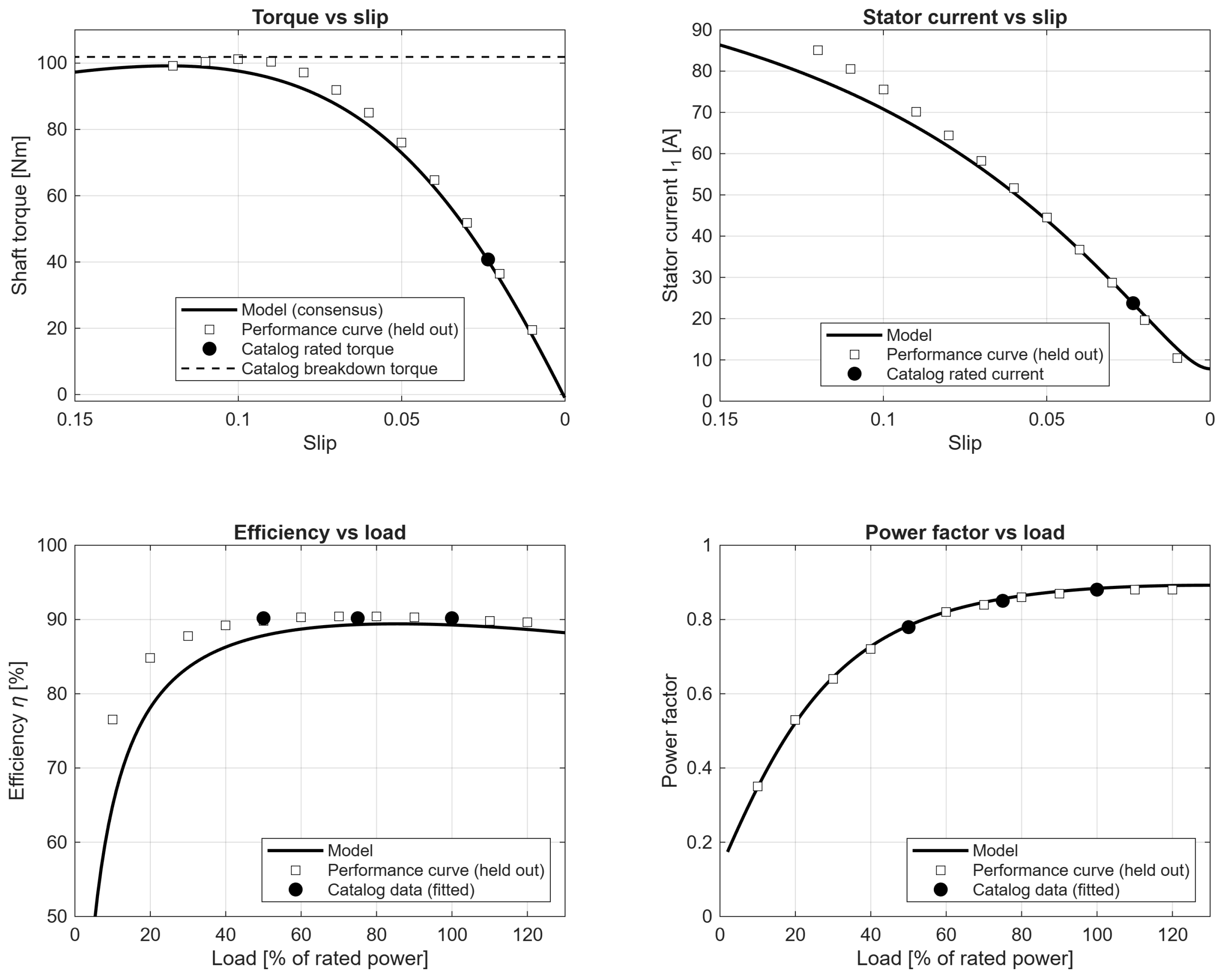
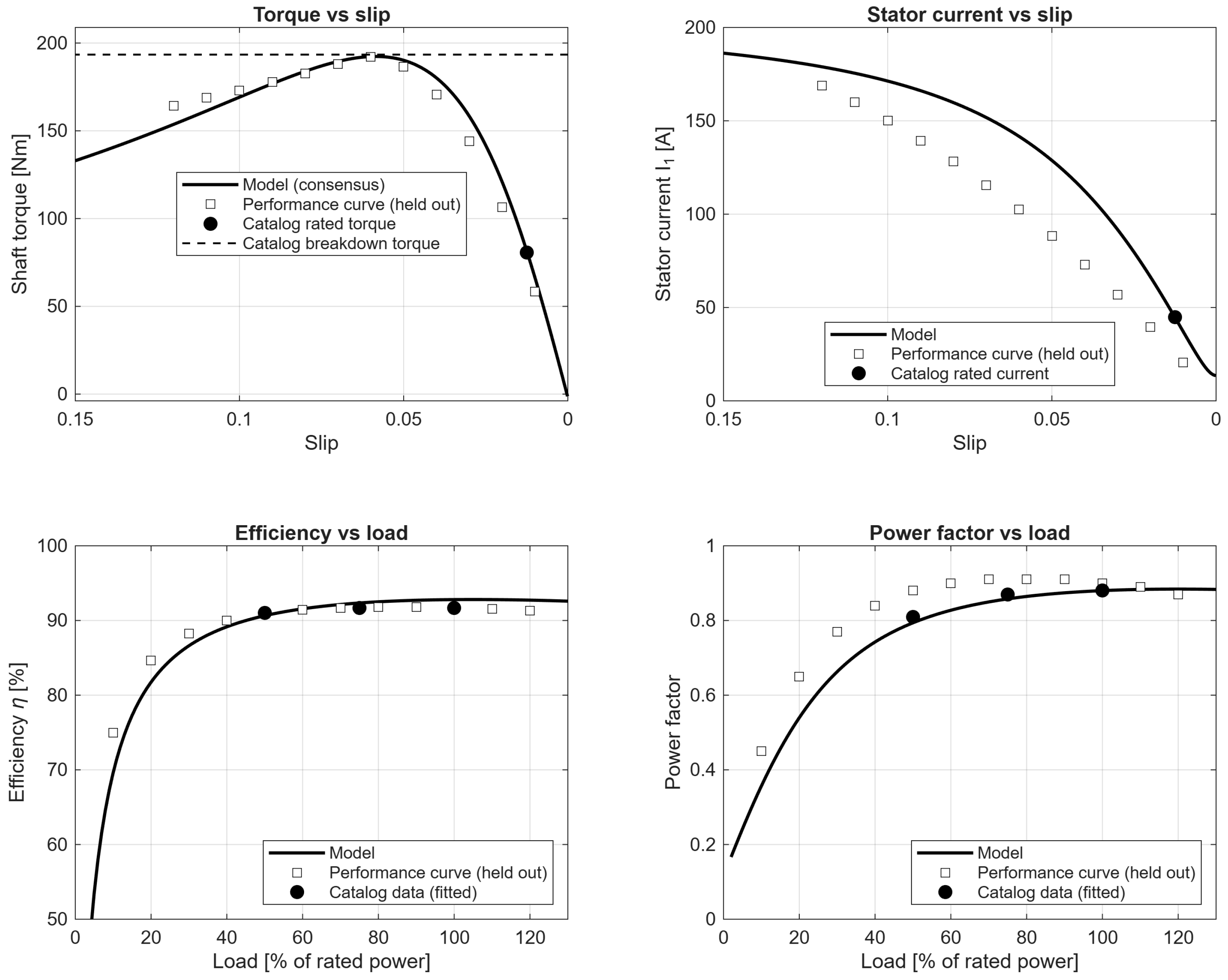
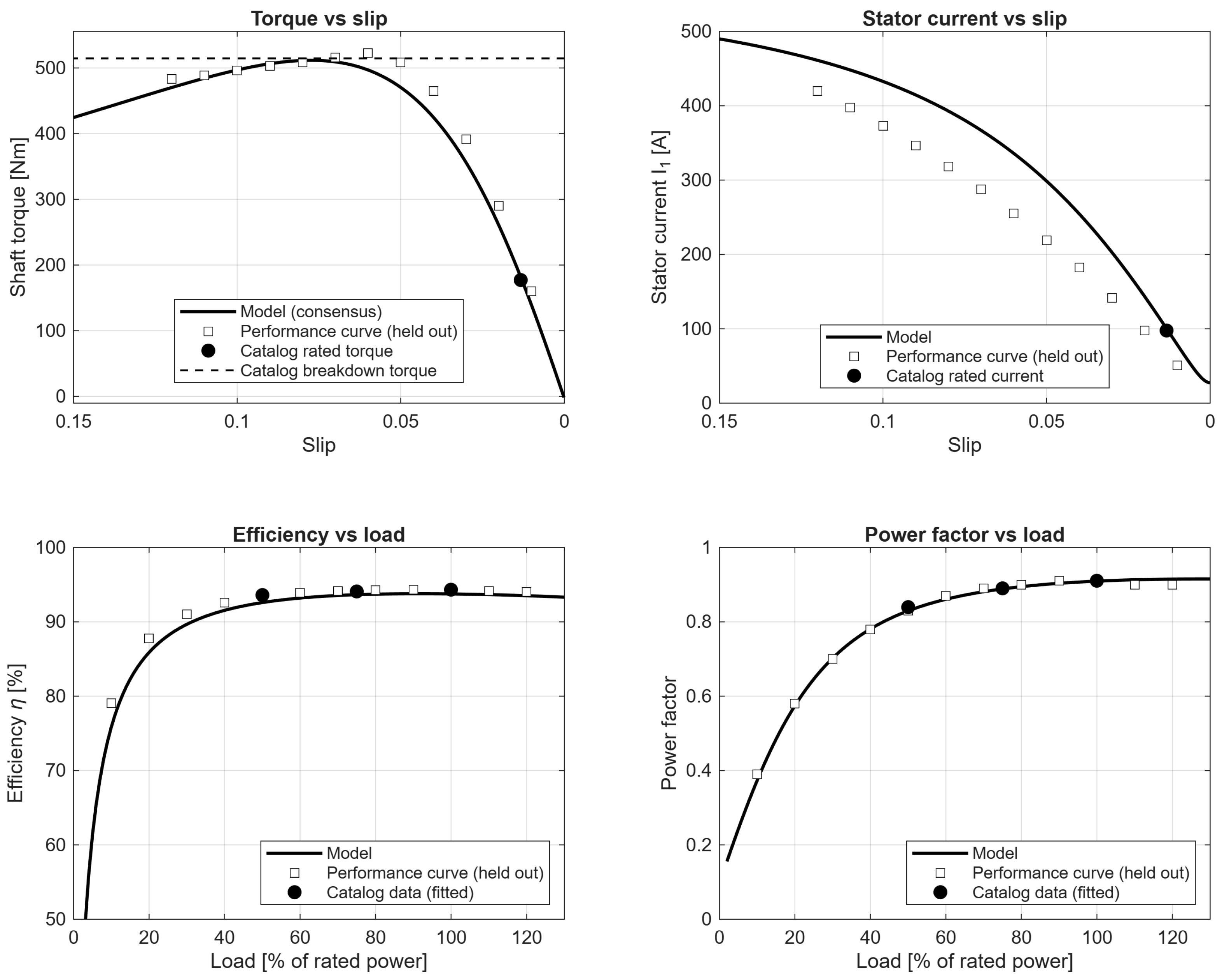
The consistency of the estimation is demonstrated by superimposing the discrete manufacturer data points onto the curves generated by the estimated equivalent circuit as shown in Figure 2, Figure 3 and Figure 4. A high degree of correlation between the reconstructed trajectories and the reported operational points indicates that the proposed framework reconstructs the catalog operating points and the manufacturer performance curves consistently. Because no laboratory parameters exist for these machines, this is a catalog-reconstruction check rather than a direct verification of parameter accuracy.

The electromechanical response under varying slip conditions in the range $s=0.15$ to $s=0.01$ allows a critical assessment of the identified reactances and resistances. In the stable low-slip region (s < 0.08), the predicted stator current aligns closely with the catalog points for all three machines. At high slip, the single-cage model systematically overestimates the current: the deviation is slight for Motor 6 (Figure 2) but becomes noticeable for Motors 7 and 8 (Figure 3 and Figure 4). This overestimation is the expected signature of neglecting deep-bar and skin effects, which raise the effective rotor resistance and reduce the actual current at high slip. A further observation concerns the curves themselves: for two of the three machines, the slip at which the manufacturer’s current curve reaches the nameplate rated current does not coincide with the nameplate rated slip. The curves and the nameplate are, therefore, published on bases that are not mutually consistent, which is precisely the situation the screening of Section 3.1 is designed to detect. The curves are consequently used here only as a qualitative consistency check and take no part in the objective at any point.

The torque-slip characteristic shows the highest level of correlation among all the measured parameters and models. For each machine, the model reproduces the catalog breakdown-torque ratio (2.4–2.9 pu) at its corresponding breakdown slip. The slope of the stable region and the location of the breakdown point are governed by the rotor resistance and the total leakage reactance, so their agreement with the catalog is consistent with those parameters having been identified correctly. It is not proof of it: no laboratory values exist for these machines, and the quantities being matched entered the objective.

The alignment between the model and the experimental data across the power spectrum is essential to validate the utility of the model in energy management and efficiency optimization studies. The reconstruction follows the catalog points closely across the load range. It successfully captures the rapid non-linear transition from a low power factor at light loads to a stabilized value of approximately $0.9$ at rated power. The agreement is close at and above rated load, while at partial load the model overestimates the power factor, as quantified in

Table 22. Catalog data (Cat.) versus the median-consensus model (Mod.) for three WEG induction motors. The no-load current takes no part in the objective and is, therefore, a blind prediction; every other row is a fitted quantity.

Variable	Motor 6 (15 kW)			Motor 7 (30 kW)			Motor 8 (55 kW)
	Cat.	Mod.	Err. %	Cat.	Mod.	Err. %	Cat.	Mod.	Err. %
Rated torque [Nm]	40.75	40.56	$-0.48$	80.59	81.45	$+1.07$	177.44	181.87	$+2.50$
Rated current [A]	23.70	23.65	$-0.21$	44.80	44.64	$-0.36$	97.40	100.34	$+3.02$
PF @100%	0.880	0.884	$+0.42$	0.880	0.880	$+0.05$	0.910	0.911	$+0.06$
$\eta$ @100%	0.902	0.896	$-0.61$	0.917	0.928	$+1.20$	0.943	0.937	$-0.59$
$T_{max}/T_{rated}$	2.500	2.465	$-1.41$	2.400	2.413	$+0.54$	2.900	2.903	$+0.09$
PF @75%	0.850	0.856	$+0.69$	0.870	0.858	$-1.40$	0.890	0.888	$-0.17$
$\eta$ @75%	0.902	0.898	$-0.45$	0.917	0.923	$+0.70$	0.941	0.937	$-0.46$
PF @50%	0.780	0.782	$+0.32$	0.810	0.794	$-2.00$	0.840	0.830	$-1.25$
$\eta$ @50%	0.902	0.885	$-1.87$	0.910	0.906	$-0.40$	0.936	0.926	$-1.06$
$I_0$ [A], blind	5.70	7.83	$+37.37$	11.50	13.59	$+18.20$	22.00	27.42	$+24.64$

and discussed below. The experimental efficiency values are closely mirrored by the model’s predictions. In particular, the model accurately identifies the peak efficiency region of the rated power. A marginal discrepancy is observed at very low loads (<$10\%$ power), where the models slightly underestimate the losses. However, for the primary operating range ($20\%$ to $120\%$ load), the models serve as a robust predictor of machine energy performance, maintaining an efficiency error margin below 1.87% and a power-factor error below 2.00%, both worst cases occurring at 50% load, as Table 22 shows.

Table 22 summarizes the reconstruction of the catalog operating point. Every fitted quantity is reproduced within 3.02%: the rated torque within 2.50%, the rated current within 3.02%, the breakdown-torque ratio within 1.41%, the power factor within 2.00% and the efficiency within 1.87%, the last two at 50% load, where the catalog resolution is coarsest relative to the quantity being matched. The no-load current is the exception, and it is not a fitted quantity: excluded from the objective, it is overestimated by 18% to 37% on the three machines. That deviation is the expected signature of a linear magnetizing branch evaluated at rated voltage, and

Table 23. No-load current as a blind prediction and as a fitted residual, and the effect of the difference on the two loss parameters. Blind: $I_0$ absent from the objective. Fitted: $I_0$ included with weight 2.

	${\mathit{I}}_0$ [A]			Change, Blind → Fitted
Motor	Catalog	Blind (Err %)	Fitted (Err %)	${\mathit{R}}_{\mathit{c}}$ [%]	${\mathit{P}}_{\mathit{rot}}$ [%]
6 (WEG 15 kW)	5.70	7.83 (+37.37)	6.26 (+9.82)	+3.39	−6.32
7 (WEG 30 kW)	11.50	13.59 (+18.20)	12.14 (+5.55)	+0.84	−0.39
8 (WEG 55 kW)	22.00	27.42 (+24.64)	23.32 (+6.02)	+0.57	−0.28

quantifies what including it as a residual would and would not buy. For the primary operating range, the identified circuits, therefore, support energy-efficiency auditing and steady-state control design; for transients, starting, or operation deep into saturation, a saturation-dependent reactance and a multiple-cage rotor remain necessary.

The no-load current deserves separate treatment, because it is the one catalog quantity that is sometimes published and that bears directly on the core-loss/rotational-loss ambiguity of Section 4.2. Table 22 reports it as a blind prediction, since it takes no part in the objective anywhere in this work. Table 23 reports what its inclusion as a residual would buy.

Two facts emerge. Blind, the no-load current is overestimated by 18% to 37%, systematically and on all three machines, which is the expected signature of a linear magnetizing branch evaluated at rated voltage. Including it as a residual reduces its own error by roughly a factor of four. But the loss parameters barely move: the core-loss resistance changes by 3.39% at most and by less than 1% on two of the three machines, and the rotational losses by 6.32% at most. The no-load current is, therefore, predominantly an observation of the magnetizing branch, not of the constant-loss split. It sharpens $X_m$; it does not resolve the $R_c$–$P_{rot}$ ambiguity, which in this framework is resolved instead by the constant-loss decomposition of Equation (29). All figures reported elsewhere in this paper are obtained with $I_0$ excluded from the objective, so the values of Table 23 are a genuine blind prediction.

4.8. Extrapolation Beyond the Calibration Range

To probe the generalization of the framework outside the power range of the calibration population, the two extended-range datasets of Section 3.1—rated at 11 kW and 115 kW (Motors 9 and 10)—were characterized from their catalog-style data with the MAP+ estimator, without re-tuning any predictor coefficient, prior dispersion, or regularization strength.

Table 24. Extrapolation beyond the calibration range: catalog reference (Cat.) versus the median-consensus model (Mod.) for the two extended-range datasets. The locked-rotor ratios take no part in the objective.

	11 kW			115 kW
Variable	Cat.	Mod.	Err. %	Cat.	Mod.	Err. %
Rated torque [Nm]	59.58	59.81	$+0.38$	1109.15	1131.82	$+2.04$
Rated current [A]	22.00	22.02	$+0.08$	120.80	122.85	$+1.69$
PF @100%	0.832	0.838	$+0.75$	0.834	0.839	$+0.58$
$\eta$ @100%	0.914	0.909	$-0.55$	0.956	0.953	$-0.33$
$T_{max}/T_{rated}$	3.010	2.956	$-1.78$	2.760	2.771	$+0.40$
PF @75%	0.776	0.784	$+1.02$	0.789	0.791	$+0.26$
$\eta$ @75%	0.919	0.910	$-1.00$	0.958	0.953	$-0.56$
PF @50%	0.662	0.673	$+1.71$	0.686	0.689	$+0.50$
$\eta$ @50%	0.914	0.898	$-1.77$	0.953	0.945	$-0.84$
$T_{st}/T_{rated}$	2.450	0.859	$-64.93$	2.440	0.319	$-86.91$
$I_{st}/I_{rated}$	8.280	5.716	$-30.97$	8.880	5.196	$-41.49$

compares the reconstructed operating quantities against the reference nameplate values, again as the median consensus over the fifteen algorithms.

The steady-state characterization extrapolates cleanly. Every running-point quantity—rated torque, rated current, power factor and efficiency at 50%, 75% and 100% load, and the breakdown-torque ratio—is reproduced within 2.04% for both machines, and thirteen of the eighteen residuals stay below 1.50%. The breakdown-torque ratio is reproduced here as a fitted quantity; Section 4.6 reports what the estimator does when the same ratio is withheld. That this accuracy is preserved at 115 kW, well above the 75 kW ceiling of the reference population and with no recalibration, indicates that the nameplate predictors and their population-calibrated dispersions capture power-invariant structure rather than dataset-specific tuning.

The starting-condition quantities, by contrast, expose the boundary of the single-cage model. The locked-rotor ratios $T_{st}/T_{rated}$ and $I_{st}/I_{rated}$ are underestimated by up to 86.91% and 41.49%, respectively. These quantities are governed by the rotor impedance at unit slip, where deep-bar and skin effects redistribute the rotor current toward the bar surface and raise the effective rotor resistance—physics that the constant-parameter single-cage circuit does not represent. Crucially, the starting ratios take no part in the objective function, which is built exclusively from running-point residuals (Section 3.5); their deviation is, therefore, a genuine out-of-model extrapolation rather than a fitting error, and it quantifies precisely the regime in which the double-cage extension identified in Section 6 becomes necessary. The framework thus reconstructs steady-state behavior accurately across a wide power range, while its predictions near standstill should be regarded as indicative only and delimit the single-cage model to running operation.

4.9. Comparison with State-of-the-Art Metaheuristics

A notable achievement of the current literature is the estimation of the rated torque ($T_{rated}$), which reached a marginal error of 0.17% for the WEG W22 15 kW machine (Table 22). In [13], the researchers found a 4.01% error in the nominal torque for a 1 kW motor, the minimum error after implementing IMFO among the six algorithms studied. It is critical to clarify that a direct numerical comparison between these two studies is subject to the difference in machine scale. The IMFO study focuses on a 1 kW laboratory-scale motor, whereas the present work analyses industrial-grade machines. However, these results provide evidence that physically constrained metaheuristic optimization can achieve estimation accuracy comparable to current state-of-the-art approaches, provided that the optimization process is guided by physically meaningful engineering constraints.

The comparison should also be read against the most recent revisions of the field. The group responsible for the baseline dataset has extended its assessment to nine estimation methods oriented toward nonintrusive loss estimation [11], and new metaheuristic variants continue to appear, including an enhanced grey wolf optimizer applied to commercial machines [16]. Both lines share a common pattern: accuracy gains are pursued mainly through new search mechanisms operating on essentially unchanged problem formulations. The ablation of Section 4.3 points to the complementary route. Upgrading the information content of the formulation itself produced a larger improvement than any algorithmic substitution, as quantified in Section 5.1.

5. Discussion

5.1. Physical Constraints as the Primary Driver of Accuracy

The present results indicate that the improved performance of the proposed framework is primarily attributable to the incorporation of physically informed constraints rather than to the choice of optimization algorithm alone. Across all tested metaheuristics, solutions obtained within the impedance-scaled search space consistently outperformed the analytical benchmark methods reported in the literature. This observation suggests that the definition of physically realistic parameter boundaries plays a more critical role than the specific search mechanism used by the optimizer.

The enforcement of IEEE Std 112 leakage reactance ratios and the impedance-based initialization strategy proved particularly effective in mitigating the well-known tendency of parameter estimation procedures to overestimate stator resistance. By restricting the search to electromagnetically plausible regions, the optimization process avoided many of the unrealistic solutions commonly observed in unconstrained formulations. These findings reinforce the importance of embedding domain knowledge directly into optimization frameworks rather than relying exclusively on algorithmic sophistication.

The ablation experiment of Section 4.3 makes this claim quantitative and constitutes, in our assessment, the central finding of this work. Exchanging the best-performing for the worst-performing algorithm in Table 4 moves the global error between 14.71% and 23.33%—a factor of about 1.6 governed by the search strategy. Exchanging the fixed-coefficient formulation for the MAP+ estimator moves the error from 14.71% to a validated 4.27% with the algorithm, the budget, and the random seeds held fixed: a larger improvement than any algorithmic substitution provides, obtained without a single additional catalog datum. The repeated-run analysis sharpens this reading. Under the fixed-coefficient formulation, the six representative algorithms differ significantly on all five reference motors; under MAP+, the same test returns $p=0.730$ and the six agree to within 0.01 percentage points. The formulation, therefore, does not merely outweigh the choice of optimizer; it removes that choice as a source of variation.

The core quantities of the MAP formulation are measured rather than hand-set—the prior means follow from circuit arguments, the prior dispersions from cross-validation, the bounds from the prior itself—while the weights, $\lambda$, and loss fractions are selected on the reference set; the gain is, therefore, attributable chiefly to information structure rather than to additional degrees of freedom. The practical reading for nameplate-based estimation is direct: effort invested in the information structure of the problem returns more than effort invested in the sophistication of the optimizer.

5.2. Practical Identifiability and the Role of the Priors

The persistent error structure diagnosed in Section 4.2 admits an interpretation in terms of practical identifiability. The catalog vector of Equation (1) supplies only nine scalar observations at fixed voltage and frequency, and is nearly degenerate along the stator-resistance and constant-loss-split directions. Any estimator confined to that data must, therefore, import external knowledge to resolve them.

The Gaussian priors of Section 3.6 supply this knowledge in proportion to how much each parameter needs it. Because the prior strength scales with $1/{\sigma }_i^2$, the estimator defers to the catalog data wherever the data are informative (on the benchmark machines, the magnetizing reactance predictor is biased by up to $+17\%$, yet the final $X_m$ estimates track the current and power-factor residuals to within 2%) and defers to the population statistics where the data are silent, as with the constant-loss split. Nothing in this mechanism is specific to induction machines; it is the standard behavior of a MAP estimator with heteroscedastic priors [20]. Its value here lies in replacing two practices the parameter-estimation literature has normalized, hand-tuned box constraints and post hoc rejection of implausible solutions, with a single construction whose prior means, dispersions and bounds are measured and reportable, and whose few remaining hyperparameters ($\lambda$ and the weights) are selected transparently on the reference set.

The held-out validation of Section 4.6 measures this mechanism from the outside. Quantities that the catalog determines are recovered when withheld: the rated current to 0.96% and the partial-load power factors to 2.65%, the latter entering no prior mean and, therefore, leaving no pathway by which the withheld value could re-enter the estimate. The breakdown-torque ratio is not recovered: withheld, it compresses toward the population-typical value, with the error correlating at $r=-0.88$ with the catalog value itself. This is the expected behavior of a MAP estimator along an unobserved coordinate, and it is also the price of the prior—accuracy on population-typical machines is bought with shrinkage of atypical ones. The three machines whose ratio is underestimated by more than 13% are precisely the three with the highest catalog values, between 2.76 and 3.01. Two mechanisms are consistent with this pattern and the present data cannot separate them: shrinkage toward the population, and the ceiling that a single-cage circuit constrained to reproduce the rated point imposes on the attainable breakdown torque. The second mechanism is the same one that governs the locked-rotor ratios of Table 24, and both point to the same conclusion for practice. Two practical consequences follow. The breakdown-torque ratio must be treated as an input rather than an output, and a calibration population broader than five machines is a precondition for applying the estimator to designs far from those sampled here.

The no-load current is the observation most often proposed as the resolution of the $R_c$–$P_{rot}$ ambiguity, on the grounds that it isolates the shunt branch. Table 23 tests that expectation and does not support it. Adding the no-load current as a residual reduces its own prediction error by about a factor of four, but displaces the core-loss resistance by no more than 3.39% and the rotational losses by no more than 6.32%, in both cases well inside the prior dispersions of Table 2. The reason is that the no-load current is governed by the magnetizing reactance far more strongly than by the loss split: it constrains where the shunt branch sits, not how the constant losses divide between its two mechanisms. What does separate them is the curvature of the efficiency–load characteristic, which is why the constant-loss decomposition of Equation (29) produces the collapse of the $P_{rot}$ bias reported in Table 11 while the no-load residual does not. The practical implication is favorable: the information needed to segregate the losses is already present in datasheets that publish partial-load efficiencies, and does not require the less commonly published no-load current.

5.3. Lessons Learned from Human–AI Collaborative Engineering

The software infrastructure was built with a Human-in-the-Loop workflow assisted by a Large Language Model, which accelerated code generation, algorithm integration, and debugging. The engineering content (circuit topology, constraints, admissible ranges, objective function, and validation) was defined and verified by the authors, who take full responsibility for it. The most consequential lesson was practical: the quality of the outcome depended far more on the completeness of the engineering constraints supplied than on prompt wording, with under-constrained early iterations producing physically inconsistent code that stabilized only as constraints were made explicit.

5.4. Implications for Engineering Practice

From an engineering perspective, the proposed methodology offers a practical alternative to conventional parameter identification procedures that require dedicated laboratory testing.

An important aspect of the validation strategy is the use of three complementary datasets. The benchmark dataset of five industrial motors was employed to quantify estimation accuracy against reference parameters reported in the literature, whereas the three WEG W22 machines served as an independent prediction dataset for which the internal equivalent-circuit parameters were unavailable, and two extended-range catalog datasets probed extrapolation beyond the power, voltage and frequency range of the calibration population (Section 4.8). Consequently, the objective of these prediction datasets was not statistical generalization across a large motor population but rather the verification that the proposed framework could reconstruct realistic operational characteristics using only manufacturer catalog information. The accurate reproduction of torque, current, power factor, and efficiency curves across these independent machines provides additional evidence of the practical applicability of the methodology.

Finally, although the validation includes benchmark motors and independent industrial machines from the WEG W22 series, the dataset remains limited in size. Future studies should extend the evaluation to larger collections of motors from multiple manufacturers and design classes to further assess the generalizability of the proposed framework.

Reconstructing an equivalent circuit from manufacturer catalog data alone supplies the steady-state layer of a digital twin—the component that converts a nameplate into a model able to predict torque, current, power factor and efficiency across the load range—in environments where IEEE Std 112 testing is unavailable, and likewise supports energy auditing, predictive maintenance planning and teaching. The held-out validation of Section 4.6 delimits that use: within the running regime, the model predicts quantities it never saw to within about 1–3%, while standstill behavior and the breakdown-torque ratio fall outside what the single-cage circuit and the present calibration can supply. A dynamic twin would require the double-cage and saturation extensions of Section 6. What this work contributes is, therefore, not a finished general-purpose tool but a demonstration, with its accuracy and its boundary both measured, that such a tool can be built on nameplate data.

6. Limitations and Future Work

6.1. Limitations

First, the methodology depends on the quality and completeness of the manufacturer catalog data, which may contain tolerances, rounded values, or incomplete operating information that introduce uncertainty into the estimation process. Second, the adopted single-cage equivalent circuit is well suited for steady-state performance analysis but may not fully capture transient phenomena, deep-bar effects, or magnetic saturation under high-slip conditions, as the large errors on the locked-rotor ratios $T_{st}/T_{rated}$ and $I_{st}/I_{rated}$ in Table 24 confirm. Third, although the physically constrained search-space formulation improves robustness, the fixed-coefficient configuration relies on expert-defined initialization heuristics and admissible ranges, whereas the MAP configurations derive both the seed and the $\pm 3\sigma$ search box from the population-calibrated priors; extending the priors to substantially different designs may still require recalibration. Consequently, the generalization of the methodology to motors with substantially different designs may require additional calibration and validation.

Fourth, the predictor coefficients, the prior dispersions, and the regularization strength of the MAP configuration were calibrated on the same five reference machines used to quantify the accuracy gains, so the ablation figures of Section 4.3 contain an optimistic component. Five machines suffice to pin down the electromagnetic coefficients, whose implied per-motor values vary by less than 5%, but they determine a standard deviation only loosely: the 95% confidence interval of a standard deviation estimated from five samples spans roughly 0.6 to 2.9 times its point value, so the loss-predictor dispersions in Table 2 should be regarded as provisional. Three mitigations apply. The $\lambda$ response is shallow, so moderate misestimation of the dispersions has limited effect on the estimates; the priors on the well-identified parameters are corroborated by the data themselves and the three WEG machines, which took no part in any calibration, reproduce catalog behavior with errors consistent with the benchmark results. A nested cross-validation over the five reference motors (Section 4.5) already removes the resubstitution optimism, re-calibrating the predictor coefficients, the dispersions, the loss-split fractions and $\lambda$ on each training fold and yielding a validated 4.27% global error; the weighting vector remains outside that loop, and Table 17 bounds its influence at under one percentage point. Extending it to a larger reference population stratified by power rating and design class remains priority future work. Fifth, the narrowed leakage-ratio interval adopted in the MAP configuration reflects the design-class distribution of the reference machines; motors of NEMA (National Electrical Manufacturers Association) design classes C and D require a different interval and, plausibly, recalibrated predictors.

Sixth, the held-out validation of Section 4.6 shows that the breakdown-torque ratio is not recoverable from the remaining nameplate data: it must be published for the estimator to be applied as described, and machines whose ratio departs markedly from the reference population are shrunk toward it. The method, therefore, presumes a reasonably complete datasheet—partial-load efficiency and power factor together with the breakdown-torque ratio—and is not applicable to a bare nameplate.

The benchmark of Section 4.1 uses a single seeded run per motor–algorithm pair, a design chosen to isolate the influence of the estimation formulation. Section 4.4 complements it with thirty independent runs of six representative algorithms under all three configurations, reporting dispersion, computational cost and a non-parametric comparison. That analysis is restricted to six of the fifteen algorithms, and the convergence traces of Table 15 to five of those six over ten seeds; extending it to the full roster, and to a reference population large enough for the classical across-problem form of the Friedman test to carry adequate power, remains open.

6.2. Future Research Directions

A fully probabilistic treatment—per-residual noise variances so that likelihood and prior share a common scale, an off-diagonal prior covariance, and calibration on a larger population—is the natural next step toward a strict empirical-Bayes estimator.

Future research should focus on the development of adaptive or meta-optimized seeding mechanisms to further reduce the reliance on manual heuristic tuning. Additionally, expanding the Polymorphic Optimization Engine to identify parameters for Double-Cage Models would enhance its utility for transient and high-starting-torque simulations. Subsequent studies should also investigate the model’s performance under non-sinusoidal supply conditions—such as those encountered in variable frequency drives (VFD)—where saturation and skin effects become more pronounced.

Regarding the framework, several refinements are proposed to further reduce the validated error and to extend the model beyond running operation:

• Initial Point Optimization: Utilizing simplified analytical estimates to provide a “warm-start” for the initial population of the metaheuristic search.
• Penalty Vector Refinement: Revision of penalty functions to enforce standard NEMA design constraints, thereby improving the consistency of the estimation.
• Double Squirrel-Cage Modeling: Expand the objective function to incorporate double-cage models, which better represent starting conditions in high-power industrial motors (cf. the starting-ratio errors in Table 24).
• Mathematical Formalization: A systematic review of hyperparameters, including the number of seeds, populations, and iterations, is planned from a formal mathematical perspective.

Finally, validation of the framework across a more diverse dataset, including multiple manufacturers and specialized motor designs, will be essential to establish the generalizability of the proposed physically constrained parameter-identification framework in industrial environments.

7. Conclusions

This study demonstrates that physically constrained metaheuristic optimization provides an effective methodology for identifying induction motor equivalent-circuit parameters from manufacturer nameplate data. The combination of impedance-based search-space initialization, IEEE Std 112 leakage-reactance constraints, and population-calibrated priors enabled significant improvements over analytical benchmark methods. The population-calibrated MAP+ estimator achieved an apparent global error of 3.48% on the calibration motors and a nested-cross-validated (validated) global error of 4.27%, against 23.40% for the best analytical method and 14.71% for the best unregularized metaheuristic.

The results confirm that the main source of accuracy improvement is the incorporation of physically informed engineering constraints into the optimization process. By scaling the search space according to the motor base impedance and enforcing admissible leakage-reactance ratios, the proposed framework reduces the risk of convergence toward mathematically valid but electromagnetically unrealistic solutions. This behavior is particularly relevant in induction motor parameter identification, where unconstrained optimization may produce inaccurate distributions of stator resistance, rotor resistance, leakage reactance, and loss components.

The assessment carried out using benchmark motors and independent WEG W22 industrial machines shows that the proposed methodology can reconstruct steady-state performance characteristics using only manufacturer catalog data. The estimated models reproduced rated torque, current, efficiency, and torque-slip behavior under rated and partial-load conditions to within 3.02%, the largest single deviation being the rated current of the 55 kW machine. Withholding catalog quantities from the estimation and predicting them back provided forty out-of-fit checks on ten machines, recovering the rated current within 0.96% and the partial-load power factors within 2.65%, while the breakdown-torque ratio proved not to be recoverable from the remaining data. These results support the framework wherever IEEE Std 112 laboratory testing is impractical—energy auditing, model-based engineering, and the steady-state layer of digital twins—within the running regime and for machines documented to the level assumed here. What the study establishes is not a general-purpose estimator but a demonstration, with its accuracy and its boundary both measured, that nameplate-based identification can be given a calibrated statistical basis; extending the calibration population across manufacturers and design classes is the step that would turn that demonstration into a general method.

Three boundaries delimit the present formulation, and each defines the work that follows from it. The single-cage circuit represents running operation accurately but not standstill, where deep-bar and skin effects redistribute the rotor current and raise its effective resistance; a double-cage extension is required before the locked-rotor quantities can be predicted rather than merely reported. The priors are diagonal Gaussians whose dispersions are estimated from five machines, so a fully probabilistic treatment—per-residual noise variances that place likelihood and prior on a common scale, an off-diagonal prior covariance, and calibration on a larger population stratified by rating and design class—would replace the single tuned regularization strength with a calibrated one. And the estimator assumes sinusoidal supply at rated voltage and frequency, so operation from a variable-frequency drive, where saturation and harmonic losses become significant, lies outside the model as constructed. Each of these is a defined extension of the framework rather than a redesign of it, which is the practical benefit of having measured where the present formulation stops.