AdaNMD: Nested Diffusion with Adaptive Resolution Decision for Efficient Industrial Anomaly Localization

Abstract

Accurate anomalous localization is a core challenge in industrial visual quality inspection. Current diffusion-based methods typically rely on single-scale reconstruction at a fixed resolution, often exhibiting limited performance on subtle or low-contrast anomalies due to the lack of hierarchical feature collaboration. We propose AdaNMD, a nested adaptive multi-resolution diffusion model that jointly optimizes accuracy and efficiency. AdaNMD constructs a three-branch nested decoding architecture. It utilizes Adaptive Group Normalization (AdaGN) to embed diffusion time steps and a top-down feature fusion module to generate semantically rich pyramid representations. Crucially, a resolution decision module dynamically evaluates image complexity, activating only the most suitable branch during inference to reduce redundant computation. To bridge the capability gap between branches, we introduce a cross-scale self-distillation mechanism where the high-resolution branch acts as a teacher for lighter branches. A unified multi-task loss function further guides the model toward robust inference policies. Experiments on the VisA and MVTec AD benchmarks demonstrate that AdaNMD achieves Area Under the Per-Region Overlap Curve (AUPRO) scores of 95.0% and 94.4%, respectively. Furthermore, compared to a baseline always using the high-resolution branch, our method improves inference speed by approximately 21%, confirming the architecture’s advantage in achieving high-precision anomaly localization and efficient inference simultaneously.

1. Introduction

In recent years, diffusion models have emerged as one of the most promising technical paradigms in industrial anomaly detection due to their strong generative capability and progressive denoising mechanism [1,2,3]. By learning the inverse process of gradually restoring clean images from noise, they can effectively model normal patterns under complex textural backgrounds, thereby enabling high-precision anomalous region localization without requiring any anomalous samples during training. Nevertheless, despite significant advances in reconstruction quality, existing methods still face a critical bottleneck in practical applications. They generally lack the ability to effectively model multi-scale contextual information and perform hierarchical feature fusion. Specifically, mainstream architectures predominantly adopt a single-scale encoder-decoder design [4,5], which struggles to jointly capture global semantic structures and local fine-grained details during feature extraction and image reconstruction. This limitation often leads to incomplete anomaly responses when dealing with anomalous regions that exhibit complex morphology, large spatial extent, or ambiguous boundaries. The problem is particularly pronounced in industrial scenarios involving multiple coexisting components or highly irregular textures, where false positives or missed detections frequently occur, severely hindering deployment in high-reliability visual inspection systems.

In addition to limited representational capacity, diffusion models also suffer from shortcomings in inference efficiency and adaptability. Although current efficient diffusion techniques have significantly accelerated the generation process, their design principles are primarily tailored for general-purpose image synthesis tasks and exhibit clear limitations when directly transferred to industrial anomaly detection scenarios. Existing acceleration strategies, such as knowledge distillation, reduced sampling steps, or static model compression, fundamentally follow a static optimization paradigm. They employ a fixed computational path and model architecture regardless of the input image complexity [6,7]. This rigid approach is particularly disadvantageous when processing industrial visual data. Simple samples are forced to undergo redundant high-cost computation, while complex samples may lose critical details due to excessive compression, making it difficult to achieve an optimal trade-off between efficiency and accuracy [8,9].

To systematically address the aforementioned challenges, this work proposes AdaNMD, an efficient nested diffusion model tailored for industrial anomaly detection. Specifically, AdaNMD first constructs a three-level nested diffusion architecture. The encoder follows a standard downsampling pathway to extract multi-scale features. These features are then processed by a feature fusion module through top-down upsampling and lateral connections to produce semantically enhanced and spatially aligned multi-scale representations. These fused features are fed into three parallel decoders that simultaneously perform reverse denoising at low, medium, and high resolutions, forming a coarse-to-fine progressive reconstruction stream. To bridge the performance gap across resolution branches, we design a multi-task self-distillation mechanism. In this mechanism, the high-resolution branch serves as the teacher, transferring fine-grained reconstruction knowledge to the medium- and low-resolution student branches via three sub-losses, namely noise distribution distillation, feature mean alignment, and anomalous mask transfer. This significantly enhances the sensitivity of the student model to subtle anomalies and complex boundaries. Building upon this, we introduce a resolution decision module to enable input-adaptive efficient inference. This lightweight subnetwork dynamically evaluates the reconstruction difficulty of the current sample based on the fused features. It then outputs routing probabilities to select the optimal decoding path. All decoder branches replace conventional convolutions with depth-wise separable convolutions, substantially reducing Floating Point Operations (FLOPs) while preserving representational capacity, thereby providing computationally efficient primitives for dynamic switching. Moreover, we propose a dynamic routing auxiliary loss that explicitly constrains the learning objective of the routing policy for the first time in industrial anomaly detection. This loss comprises three novel sub-losses, namely efficiency loss, confidence loss, and load-balancing loss. The efficiency loss encourages the model to balance accuracy against computational cost. The confidence loss suppresses erroneous path assignments in low-confidence regions. The load-balancing loss prevents branch activation collapse. Together, these components ensure consistency and robustness of the dynamic mechanism during both training and inference. Through this multi-level design, AdaNMD achieves an organic integration of global semantic understanding, local detail recovery, and on-demand computation scheduling within a unified framework.

In summary, the main contributions of this work are as follows:

• AdaNMD is proposed as a novel nested diffusion architecture that achieves coarse-to-fine progressive reconstruction through a three-branch decoding pathway. In this framework, all branches are fully activated during training, while only one branch is dynamically selected at inference time. The encoder incorporates Adaptive Group Normalization to embed diffusion time-step information into feature modulation, and the feature fusion module leverages an enhanced top-down Feature Pyramid Network (FPN) structure to effectively aggregate multi-scale semantics and spatial details.
• A cross-scale self-distillation mechanism is introduced within AdaNMD, with the high-resolution branch serving as the teacher and the medium- and low-resolution branches acting as students. Furthermore, a unified multi-task loss function is designed to integrate multi-scale supervision, multi-task self-distillation, and dynamic routing, explicitly guiding the model toward learning an efficient and robust inference strategy.
• AdaNMD integrates a lightweight resolution decision module that combines depth-wise separable convolutions with dynamic routing to enable input-adaptive efficient inference. This design significantly reduces redundant computation while preserving high-precision anomaly localization performance.

We conducted extensive experiments on two standard and challenging industrial anomaly detection benchmarks, VisA [10] and MVTec AD [11]. The results show that the proposed method achieves state-of-the-art performance in pixel-level anomaly localization, attaining Area Under the Per-Region Overlap Curve (AUPRO) of 95.0% and 94.4%, respectively. Moreover, compared with a baseline that always uses the high-resolution branch, AdaNMD improves inference speed by approximately 21%, clearly demonstrating the significant advantage of the proposed nested adaptive multi-resolution architecture in simultaneously achieving high-precision anomaly localization and efficient inference.

2. Related Work

Currently, a large body of work has been devoted to applying diffusion models to industrial anomaly detection tasks. These approaches primarily fall into two categories, including reconstruction-based methods and density-based methods.

Reconstruction-based methods constitute the dominant paradigm for applying diffusion models to industrial anomaly detection [1,12]. They can be further categorized into three types, namely basic reconstruction, latent-space reconstruction, and conditional reconstruction. The core idea of basic reconstruction is to train the model exclusively on normal samples so that it learns a strong prior over the normal data distribution. During testing, anomalous regions, which deviate from this normal manifold, cannot be accurately reconstructed, leading to significant discrepancies between the input image and its reconstruction. This discrepancy is then used as the basis for anomalous region localization [13]. To enhance the sensitivity of reconstruction errors to anomalies, subsequent studies have introduced semantic-level modeling mechanisms. For instance, ODD [14] designs a semantic similarity network combined with an anomaly exposure strategy to quantify the distributional shift between the input and the denoised output, thereby achieving high-precision unsupervised anomaly detection. Latent-space reconstruction first maps the input image into a compact latent space using a pre-trained encoder, performs the diffusion denoising process in this low-dimensional space, and finally reconstructs the denoised latent representation back to pixel space via a decoder [15]. This strategy not only reduces computational complexity but also enables the model to focus on more discriminative feature representations. Building upon this, NGLS-Diff [2] constructs a latent space specifically designed to capture the distribution of normal temporal patterns, overcoming the limitation of existing diffusion models that struggle to accurately reconstruct normal sequences in the raw numerical space, thus significantly improving performance in time-series anomaly detection. Similarly, DiffRec [16] proposes a cluster-aware latent-space diffusion model based on item clustering, which preserves personalized user interaction signals during denoising and effectively addresses challenges in recommendation scenarios such as high prediction overhead at scale and dynamically evolving user preferences. Conditional reconstruction improves reconstruction fidelity by incorporating additional guidance signals to constrain the diffusion process, ensuring that the output strictly conforms to a known normal prior and thereby more precisely exposing anomalies [17,18,19]. The key challenge in this line of work lies in designing effective conditioning signals that strengthen the modeling of normal patterns. For example, FDAE [4] proposes a flow-guided diffusion autoencoder that fuses foreground object appearance and optical flow motion cues to construct a condition-guided diffusion autoencoder. Within an unsupervised framework, it jointly models appearance and motion characteristics for video anomaly detection and further enhances learning of prototypical normal features through a sample refinement strategy and a Gaussian mixture clustering network.

Density-based methods characterize anomalies through probabilistic modeling, typically assuming that anomalous samples reside in low-density regions of the normal data distribution [3]. This category includes score-based methods and diffusion-time-estimation methods. Score-based methods leverage the score function, defined as the gradient of the log probability density. During the reverse denoising process, the model produces more accurate score estimates for normal regions, whereas estimates for anomalous regions exhibit larger deviations [20]. By accumulating score prediction errors or uncertainties along the denoising trajectory, one can quantify the local degree of anomaly [21]. To improve the reliability of score estimation and gain deeper insight into the generative dynamics, recent studies have begun conducting theoretical analyses of the diffusion process. For example, Deveney et al. [22] systematically investigated the discrepancy between the dynamics of ordinary differential equations (ODEs) and stochastic differential equations (SDEs) in score-based diffusion models through the Fokker–Planck equation. They proposed using the Fokker–Planck residual as a training regularizer, which effectively narrows the gap between the distributions generated by ODEs and SDEs solvers. This approach not only enhances ODEs sampling quality but also reveals an inherent trade-off between ODEs and SDEs sample fidelity. Diffusion-time-estimation methods are grounded in the observation that noisy versions of normal samples allow more accurate inference of their corresponding noise level, or time step t, whereas anomalous samples due to structural or textural inconsistencies lead to greater difficulty in time-step prediction [5]. Consequently, by training a time-step predictor and using its prediction error as an anomaly score, one can effectively identify subtle yet structurally anomalous regions. This perspective reframes anomaly detection as a measure of internal consistency within the diffusion process, offering a novel discriminative signal under unsupervised settings. Following this direction, DTE [23] estimates the time distribution of an input sample across the diffusion trajectory and uses its mean or mode as the anomaly score. This strategy significantly improves inference efficiency while surpassing the detection performance of conventional DDPM.

Diffusion-based methods have achieved significant progress in anomaly detection in recent years. To comprehensively evaluate the model’s performance, this paper selects this line of research, along with other mainstream works in the field, for comparative analysis. To overcome the identity mapping problem inherent in traditional reconstruction methods, DiffAD [24] introduces Latent Diffusion Models combined with noisy condition embedding to enhance the utilization of global information. Building upon this, VLMDiff [25] further leverages detailed textual descriptions extracted from Vision-Language Models as additional conditions, guiding the model to learn more robust representations of normal features. In terms of inference efficiency and paradigm innovation, InvAD [26] proposes an inversion-based, reconstruction-free detection paradigm that directly computes anomaly scores via few-step backward diffusion in the latent space, significantly boosting inference speed. Meanwhile, TransFusion [27] designs a transparency-driven diffusion process, simultaneously achieving anomaly restoration and localization by iteratively increasing the transparency of anomalous regions. Furthermore, addressing the challenges of detail preservation and adaptability during reconstruction, LASB [28] utilizes a Latent Schrödinger Bridge to achieve smooth anomaly-to-normal translation while maintaining structural integrity. GLAD [29] introduces global and local adaptive strategies, predicting optimal denoising steps and employing spatial-adaptive feature fusion to retain normal texture details and achieve high-quality anomaly restoration.

3. Method

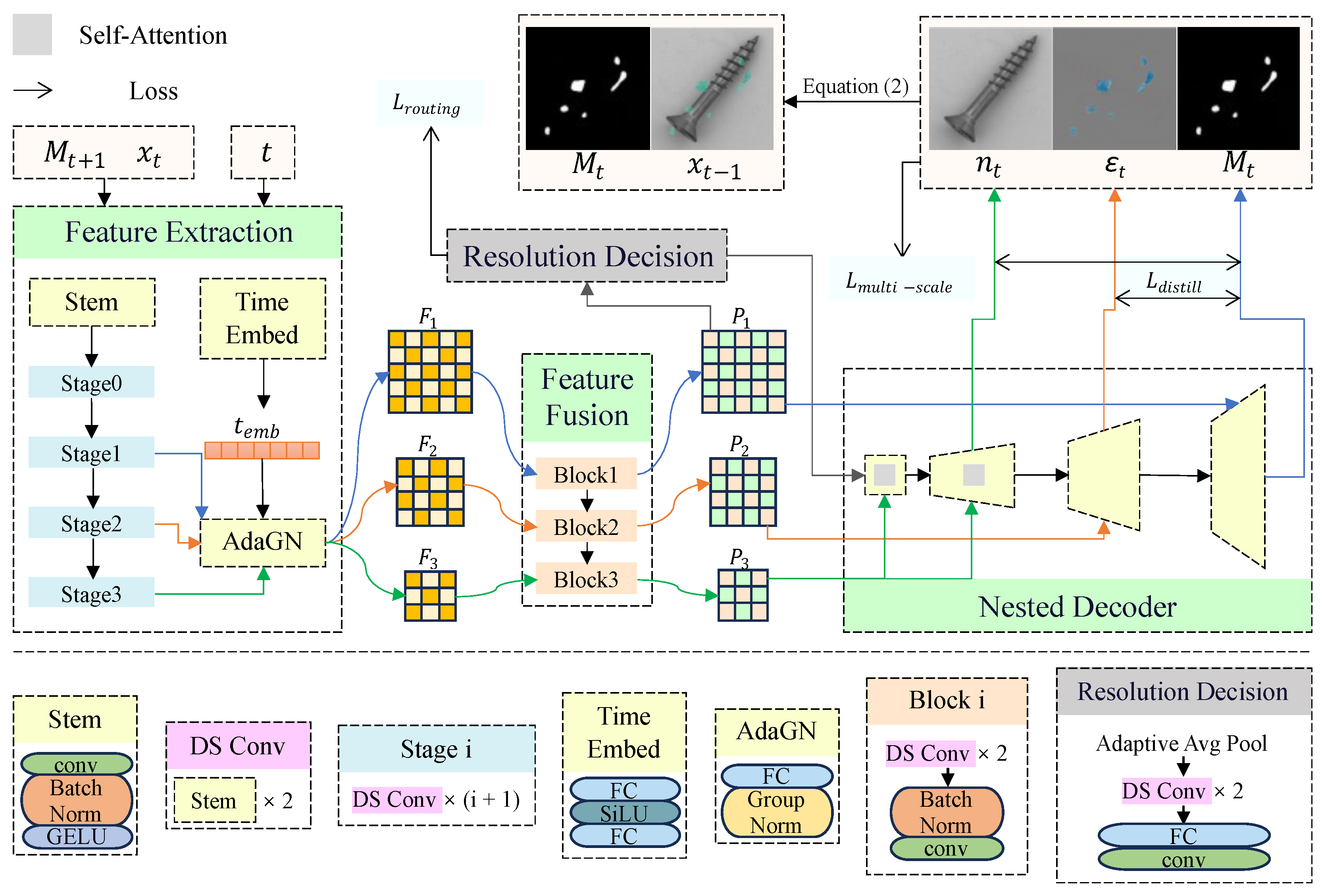
As illustrated in Figure 1, the proposed AdaNMD model comprises a feature extraction module, a feature fusion module, a resolution decision module, and a nested decoder module. These modules interact seamlessly to ensure both efficient processing and accurate detection of industrial anomalies. In brief, the diffusion time step t, the anomaly mask from the previous denoising step $M_{t+1}$, and the current noisy image $x_t$ are first processed by the feature extraction module to produce multi-scale feature representations. These features are then enhanced by the feature fusion module to enrich semantic content. Based on this enriched representation, the resolution decision module evaluates local complexity and selects the optimal decoding path. Finally, the selected decoder branch outputs the prediction for the next denoising step.

To jointly optimize anomaly localization accuracy and inference efficiency, we propose a staged multi-task unified loss function consisting of three components. The first component is the multi-scale supervision loss ${\mathcal{L}}_{multi-scale}$, which serves as the base training signal. It is applied simultaneously across the low-, medium-, and high-resolution branches, imposing four constraints: noise prediction, anomaly mask generation, image reconstruction, and temporal consistency. The second component is the multi-task self-distillation loss ${\mathcal{L}}_{distill}$. Here, the high-resolution branch acts as the teacher, providing triple soft supervision via noise distribution, feature statistics, and anomaly masks to guide the medium- and low-resolution student branches. This enhances their sensitivity to fine details and improves cross-scale semantic consistency. The third component is the dynamic routing auxiliary loss ${\mathcal{L}}_{routing}$, which explicitly optimizes the computational allocation strategy during inference. It comprises three sub-objectives: efficiency loss, confidence loss, and load-balancing loss. Together, they encourage the model to learn an intelligent single-path decision mechanism that processes simple samples rapidly while performing refined analysis on complex ones.

3.1. Nested Diffusion Model

The input to the feature extraction module is the triplet $(t,M_{t+1},x_t)$. This module first encodes the time step t into a time embedding vector $t_{emb}$, which is then injected into each stage of the encoder via Adaptive Group Normalization (AdaGN). The module consists of an initial feature extraction layer (Stem) followed by three hierarchical stages (Stage1, Stage2, Stage3). The Stem layer performs preliminary downsampling and channel expansion on the input $x_t$. Stage1 extracts high-resolution shallow features to preserve fine spatial details, and its AdaGN-modulated output is denoted as $F_1$. Stage2 integrates local structural cues with mid-level semantic information to produce an intermediate representation, yielding $F_2$ after AdaGN. Stage3 further abstracts high-level features to capture global contextual dependencies, and its AdaGN-enhanced output is denoted as $F_3$. All convolutional operations employ depth-wise separable convolutions to reduce computational cost [30]. Notably, the scaling factor $\gamma$ and shift term $\delta$ in AdaGN are dynamically generated from $t_{emb}$, enabling adaptive modulation of feature distributions across different denoising stages. The transformation is formulated as follows:

$$\mathrm{AdaGN}(x,t_{emb})=\gamma \left(t_{emb}\right)\odot \mathrm{GN}\left(x\right)+\delta \left(t_{emb}\right)$$

(1)

Here, ⊙ denotes element-wise multiplication, and GN refers to Group Normalization [31]. The input x corresponds to the shallow, intermediate, and high-level features extracted by Stage1 through Stage3, respectively. Since the diffusion process exhibits strong time dependence, with early time steps dominated by high noise levels and later steps converging toward stable reconstructions, the injection of time-conditioned signals via AdaGN enables the model to dynamically adjust feature response magnitudes according to the characteristics of each denoising stage. This significantly enhances the robustness and controllability of the entire encoding process. In the early diffusion stages, $\gamma$ may be small to suppress noise propagation, whereas in later stages, $\gamma$ increases to strengthen fine-detail reconstruction capability.

The resulting three sets of features $\{F_1,F_2,F_3\}$ are then fed into the feature fusion module, which outputs a fused feature pyramid $\{P_1,P_2,P_3\}$ that jointly preserves high spatial precision and rich semantic content. Subsequently, the resolution decision module takes the high-resolution fused feature $P_1$ as input and computes a scalar complexity score $s\in [0,1]$.

Finally, the decoder module takes the complexity score s (see Section 3.3 for details) and the deep fused feature $P_3$ as input to perform dynamic decoding. The module contains a shared intermediate processing layer followed by three dedicated decoder branches, corresponding to low-, medium-, and high-resolution output scales, respectively. Based on the value of s, the model dynamically selects exactly one decoding path for inference. If s is low, the low-resolution decoder is activated. If s is medium, the medium-resolution decoder is activated. If s is high, the high-resolution decoder is activated. The selected decoder produces three outputs, namely the anomaly mask $M_t$, the predicted anomalous noise ${\epsilon }_t$, and the denoised image $n_t$ at the current time step. These three outputs are then fused to form the final output of the model, which serves as the anomaly mask $M_t$ and the noisy image $x_{t-1}$ for the next denoising iteration. Notably, inspired by TransFusion [27], we introduce a transparency coefficient ${\beta }_t\in [0,1]$ to control the blending ratio between the normal appearance $n_t$ and the anomalous appearance ${\epsilon }_t$. The coefficient ${\beta }_t$ is defined as a monotonically increasing time scheduling function. The fusion formula is as follows:

$$x_{t-1}=x_t-({\beta }_t-{\beta }_{t-1})(M_t\odot ({\epsilon }_t-n_t))$$

(2)

During decoding, the primary input to each higher-resolution decoder does not come directly from the encoder but rather from the upsampled output of the preceding lower-resolution decoder, thereby establishing a closed-loop feedback mechanism in which lower levels guide higher ones. For example, the medium-resolution decoder takes the upsampled output of the low-resolution decoder as input, while the high-resolution decoder refines its prediction based on the output of the medium-resolution decoder. In addition, the decoder incorporates skip connections that feed the corresponding fused features $\{P_1,P_2,P_3\}$ from the encoder into their respective decoder stages. This recovers spatial details lost during downsampling and significantly improves reconstruction fidelity. Regardless of which branch is activated, its final output is upsampled to the original input resolution of $256\times 256$ via bilinear interpolation or sub-pixel convolution to ensure interface consistency. For unselected branches, computation is entirely skipped, and only the output of the currently optimal path is retained, enabling true on-demand inference.

3.2. Feature Fusion Module

To effectively integrate semantic information and spatial details from different encoder levels, the proposed model adopts an enhanced top-down FPN [32] as the feature fusion module. This module takes the three sets of multi-scale features $\{F_1,F_2,F_3\}$ produced by the feature extraction module as input, where $F_1$, $F_2$, and $F_3$ correspond respectively to shallow, intermediate, and high-level feature maps at high, medium, and low resolutions. Their spatial dimensions progressively decrease while their semantic abstraction level gradually increases. The fusion process begins with the deepest feature. Specifically, $F_3$ is directly used as the top-level fused feature $P_3$.

$$P_3=F_3$$

(3)

Next, $P_3$ is upsampled via bilinear interpolation to match the spatial resolution of $F_2$, and the result is added element-wise to $F_2$. The resulting sum is processed by a depth-wise separable convolution block to produce the second fused feature $P_2$.

$$P_2=\mathrm{DSConv}(\mathrm{Upsample}\left(P_3\right)+F_2)$$

(4)

where $\mathrm{DSConv}(·)$ denotes a depth-wise separable convolution operation. Its structure consists of a channel-wise spatial convolution followed by a point-wise channel transformation convolution, and then batch normalization and GELU activation are applied sequentially. This design significantly reduces both parameter count and computational cost while maintaining strong feature representation capability [33].

Similarly, $P_2$ is upsampled to the spatial resolution of $F_1$, added element-wise to $F_1$, and then processed once more by $\mathrm{DSConv}(·)$ to yield the first fused feature $P_1$.

$$P_1=\mathrm{DSConv}(\mathrm{Upsample}\left(P_2\right)+F_1)$$

(5)

This top-down fusion mechanism enables high-level semantics to progressively guide low-level details. As a result, $P_1$ retains original high-frequency structures such as edges, corners, and fine textures while incorporating reliable global semantic priors, making it a critical discriminative basis for the subsequent resolution decision module. All upsampling operations employ bilinear interpolation to avoid introducing additional learnable parameters. The extensive use of depth-wise separable convolutions significantly improves computational efficiency without compromising model performance, aligning well with the real-time demands of industrial deployment. The module ultimately outputs a fused feature pyramid $\{P_1,P_2,P_3\}$, with each level serving a distinct role. $P_1$ is used for complexity evaluation and as a skip connection input to the high-resolution decoder. $P_2$ is supplied to the medium-resolution decoder. $P_3$ serves not only as the initial input to the low-resolution decoder but also participates in the lowest-level skip connection. Throughout the entire fusion process, strict spatial alignment is maintained across all scales. This ensures geometric accuracy in anomaly localization and effectively prevents boundary blurring or missed detections caused by feature misalignment, thereby providing a robust and consistent feature foundation for multi-scale supervision and dynamic decoding.

3.3. Resolution Decision Module

To enable intelligent allocation of computational resources during inference, the proposed model incorporates a lightweight resolution-adaptive decision module. Its primary objective is to dynamically select the optimal decoding path based on the local complexity of the input image, thereby significantly reducing average computational cost while preserving detection accuracy. This module takes the high-resolution fused feature $P_1$ from the feature fusion module as input, as $P_1$ offers both rich spatial detail and strong semantic discriminability. It first compresses $P_1$ into a channel-wise global statistics vector via Global Average Pooling. This vector is then passed through a compact subnetwork [34] composed of two depth-wise separable convolution layers followed by a fully connected layer. The subnetwork outputs a scalar value $s\in [0,1]$, referred to as the complexity score. This score reflects the textural complexity, structural regularity, and potential difficulty of detecting anomalies in the current image region. A lower score indicates simple structure and easily identifiable anomalies, whereas a higher score suggests the presence of dense textures, ambiguous boundaries, or mixed-type anomalous patterns, which pose greater detection challenges. Based on this complexity score s, the system performs hard-routing dynamic decision making. Specifically, two fixed thresholds ${\tau }_1=0.2$ and ${\tau }_2=0.5$ are predefined to partition input samples into three categories.

$$\mathrm{Resolution}\mathrm{Path}=\left\{\begin{array}{cc}\mathrm{Low},\hfill & \mathrm{if}s<{\tau }_1,\hfill \\ \mathrm{Medium},\hfill & \mathrm{if}{\tau }_1\le s\le {\tau }_2,\hfill \\ \mathrm{High},\hfill & \mathrm{if}s\ge {\tau }_2.\hfill \end{array}\right.$$

(6)

For samples with a complexity score below ${\tau }_1$, only the low-resolution decoder is activated to enable fast reconstruction. For samples with a score between ${\tau }_1$ and ${\tau }_2$, the medium-resolution decoder is engaged to balance accuracy and speed. For samples with a score greater than or equal to ${\tau }_2$, the full high-resolution decoder is launched to perform refined anomaly restoration and precise localization. This decision process is entirely driven by internal feature representations, requiring no additional annotations or handcrafted rules, thereby realizing an efficient on-demand computation strategy. Notably, despite employing a hard-routing strategy in which only a single decoding path is active during inference, the module remains end-to-end trainable during the training phase. Specifically, the generation of the complexity score is continuous and differentiable, while the discrete routing operation is approximated using the Gumbel-Softmax trick [35] to enable gradient flow, ensuring the entire system retains full trainability.

3.4. Unified Multi-Task Loss Function

To jointly optimize high-precision anomaly localization and efficient inference, the proposed model employs a staged multi-task unified loss function. The total loss is composed of three components, namely the multi-scale supervision loss ${\mathcal{L}}_{multi-scale}$, the multi-task self-distillation loss ${\mathcal{L}}_{distill}$, and the dynamic routing auxiliary loss ${\mathcal{L}}_{routing}$. Their weighted sum is defined as follows:

$${\mathcal{L}}_{total}={\mathcal{L}}_{multi-scale}+{\mathcal{L}}_{distill}+{\mathcal{L}}_{routing}$$

(7)

Notably, ${\mathcal{L}}_{distill}$ is activated only after epoch 100, and ${\mathcal{L}}_{routing}$ is introduced after epoch 200, implementing a progressive learning strategy. During training, all encoder branches are active, meaning the low-, medium-, and high-resolution decoding paths are simultaneously enabled.

3.4.1. Multi-Scale Supervision Loss

This loss serves as the foundational supervision signal during training and is computed independently at each activated resolution level $i\in R$, where $R=\{l,m,h\}$ represents the low, medium, and high resolutions, respectively. It comprises four carefully designed sub-losses that jointly encourage the model to develop anomaly-aware perception, accurate noise modeling, and high-fidelity content reconstruction capabilities.

At the heart of diffusion models lies the ability to accurately predict the noise injected during the forward noising process. To this end, the mean squared error (MSE) between the predicted noise ${\widehat{\epsilon }}_t^i$ and the ground truth noise label ${\epsilon }_t^{true}$ of the model is minimized, as formalized by the following noise prediction loss function:

$${\mathcal{L}}_{\epsilon }^i={∥{\widehat{\epsilon }}_t^i-{\epsilon }_t^{true}∥}_2^2$$

(8)

This loss enables the model to learn anomaly-specific perturbation patterns and serves as the foundation for subsequent mask generation and image reconstruction.

To enhance localization accuracy and boundary continuity for small-scale anomalies, we combine Focal Loss [36] with Smooth L1 Loss [37]. Focal Loss alleviates the class imbalance between foreground and background pixels, which commonly arises because anomalous regions are typically sparse, while Smooth L1 provides greater robustness to gradient variations near object boundaries, as formalized by the following combined mask loss function:

$${\mathcal{L}}_M^i=\mathrm{FocalLoss}({\widehat{M}}_t^i,M_t^{gt})+\mathrm{SmoothL}1({\widehat{M}}_t^i,M_t^{gt})$$

(9)

Here, $M_t^{gt}$ denotes the binary mask ground truth generated by synthesizing pseudo-anomalies using CutPaste [38], and ${\widehat{M}}_t^i$ represents the mask predicted by the model.

To preserve the integrity of non-anomalous regions, the denoised image ${\widehat{n}}_t^i$ is required to be highly consistent with the original normal image $x_0$ in both structure and pixel-level appearance. This is achieved by jointly optimizing Structural Similarity (SSIM) [39] and L1 loss, as formalized by the following reconstruction fidelity loss:

$${\mathcal{L}}_r^i=1-\mathrm{SSIM}({\widehat{n}}_t^i,x_0)+{∥{\widehat{n}}_t^i-x_0∥}_1$$

(10)

SSIM ensures global structural fidelity, while L1 loss constrains local pixel accuracy.

Based on the inverse dynamics of the diffusion process, the model should accurately infer the image at the previous time step ${\widehat{x}}_{t-1}^i$ from the current state $x_t$ and the predicted noise ${\widehat{\epsilon }}_t^i$. This inferred image should be aligned with the actual forward process-generated image $x_{t-1}$ using MSE, which is mathematically defined as the following consistency loss:

$${\mathcal{L}}_c^i={∥{\widehat{x}}_{t-1}^i-x_{t-1}∥}_2^2$$

(11)

This loss enhances training stability and ensures the model follows a physics-informed denoising trajectory.

The four sub-losses are combined via weighted summation to form the final multi-scale supervision loss:

$${\mathcal{L}}_{\mathrm{multi}\text{-}\mathrm{scale}}=\sum _{i\in R}\left({\mathcal{L}}_{\epsilon }^i+{\mathcal{L}}_M^i+{\mathcal{L}}_r^i+{\mathcal{L}}_c^i\right)$$

(12)

Following the established paradigms in seminal works such as DRAEM [40] and TransFusion [27], we uniformly set the weighting coefficients for all sub-loss terms in Equation (12) to 1. This configuration is justified by the fact that these loss components naturally reside within the same order of magnitude under normalized inputs, thereby eliminating the need for additional scaling factors to balance their gradient contributions.

3.4.2. Multi-Task Self-Distillation Loss

The high-resolution branch, owing to its superior detail perception capability, provides high-quality soft labels and structural priors. The medium- and low-resolution branches act as students that, under a lightweight design constraint, absorb knowledge from the teacher to enhance their performance in challenging scenarios such as small-scale anomalies and edge-blurred regions.

A noise distillation loss is designed to transfer the ability of the teacher to model uncertainty in the noise distribution through these soft labels, as formulated in Equation (13).

$${\mathcal{L}}_{ϵ}^{distill}=\sum _{i\in \{l,m\}}{D}_{KL}\left(\mathrm{softmax}\left({\displaystyle \frac{{\widehat{\epsilon }}_t^h}{T_{\epsilon }}}\right)\parallel \mathrm{softmax}\left({\displaystyle \frac{\mathrm{Upsample}\left({\widehat{\epsilon }}_t^i\right)}{T_{\epsilon }}}\right)\right)$$

(13)

Here, $D_{KL}$ denotes the Kullback-Leibler Divergence [41]. ${\widehat{\epsilon }}_t^h$ is the noise predicted by the teacher (high-resolution) branch, and $\mathrm{Upsample}\left({\widehat{\epsilon }}_t^i\right)$ is the result of bilinearly upsampling the low-resolution prediction ${\widehat{\epsilon }}_t^i$ of the student branch to the high-resolution scale. The temperature parameter $T_{\epsilon }=max(4·0.{98}^E,3)$ decays with training epoch E, encouraging smooth distribution matching in early stages and sharp predictions in later phases. To align high-level semantic distributions, this work further introduces a feature mean distillation loss, which is defined as follows:

$${\mathcal{L}}_{\mu }^{distill}=\sum _{i\in \{l,m\}}{D}_{KL}\left(\mathrm{softmax}\left({\displaystyle \frac{{\mu }^h}{T_{\mu }}}\right)\parallel \mathrm{softmax}\left({\displaystyle \frac{{\mu }^i}{T_{\mu }}}\right)\right)$$

(14)

Here, ${\mu }^h$ and ${\mu }^i$ represent the channel-wise mean vectors of the teacher and student feature maps, respectively, with a fixed temperature $T_{\mu }=3$. To enhance spatial localization consistency, this study employs a mask distillation loss, as follows:

$${\mathcal{L}}_M^{distill}=\sum _{i\in \{l,m\}}\mathrm{BCE}\left(\sigma ({\widehat{M}}_t^h),{\widehat{M}}_t^i\right)$$

(15)

Here, $\sigma (·)$ converts the teacher mask ${\widehat{M}}_t^h$ into a probability map used as a soft label, and ${\widehat{M}}_t^i$ denotes the student mask. Binary cross-entropy (BCE) [42] directly supervises their localization alignment. The three distillation losses are combined using empirical weights, as follows:

$${\mathcal{L}}_{distill}=w_{\epsilon }{\mathcal{L}}_{\epsilon }^{distill}+w_{\mu }{\mathcal{L}}_{\mu }^{distill}+w_M{\mathcal{L}}_M^{distill}$$

(16)

The default settings are $w_{\epsilon }=5000$, $w_{\mu }=8000$, and $w_M$ = 10,000, emphasizing the priority of localization accuracy and semantic transfer. Following the widely adopted practice in multi-task optimization [43], these coefficients are calibrated to maintain the auxiliary routing losses within 10–20% of the primary task’s loss scale. This balance allows the model to achieve intelligent scheduling during inference while ensuring that the additional constraints do not destabilize the training process or degrade the primary detection accuracy.

3.4.3. Dynamic Routing Loss

To optimize computational efficiency and routing robustness during inference, this study introduces a dynamic-routing auxiliary loss after epoch 200 of training. This loss acts on the complexity score s produced by the resolution decision module and aims to guide the model toward learning a practical and efficient single-path selection mechanism suitable for real-world deployment.

First, to control average computational cost, an efficiency loss is introduced:

$${\mathcal{L}}_{eff}={\mathbb{E}}_x\left[\sum _{i\in R}{p}_i\left(x\right)F_i\right]$$

(17)

Here, $p_i\left(x\right)$ denotes the probability that sample x is routed to the i-th branch, and $F_i$ represents the estimated FLOPs of the i-th branch.

Second, to reduce the risk of misrouting in ambiguous decision regions, this study designs a confidence loss:

$${\mathcal{L}}_{conf}={\mathbb{E}}_x\left[\underset{k\in \{1,2\}}{min}|s\left(x\right)-{\tau }_k|\right]$$

(18)

Here, ${\tau }_1=0.2$ and ${\tau }_2=0.5$ are predefined thresholds, and this loss encourages the complexity score to stay away from decision boundaries. Finally, to prevent imbalanced resource allocation such as prolonged inactivity of a particular branch, this study introduces a load-balancing loss:

$${\mathcal{L}}_{bal}=D_{KL}\left(q\parallel \overline{p}\right)$$

(19)

Here, $q=[0.2,0.3,0.5]$ denotes the target activation frequency distribution, and $\overline{p}={\mathbb{E}}_x\left[p_i\left(x\right)\right]$ represents the actual average activation probability of the i-th branch. The three auxiliary losses are combined via weighted summation:

$${\mathcal{L}}_{routing}={\lambda }_{eff}{\mathcal{L}}_{eff}+{\lambda }_{conf}{\mathcal{L}}_{conf}+{\lambda }_{bal}{\mathcal{L}}_{bal}$$

(20)

The default settings are ${\lambda }_{eff}=0.04$, ${\lambda }_{conf}=0.05$, and ${\lambda }_{bal}=0.1$. These values are determined based on the multi-task learning principles established by Kendall et al. [43], which suggest that auxiliary losses should be scaled to approximately 10–20% of the primary loss magnitude to prevent gradient dominance. Although all branches are active in parallel during training, this loss framework effectively guides the model to achieve intelligent scheduling at inference time, enabling fast processing for simple samples and refined analysis for complex ones. This strategy balances high-precision anomaly detection and low-latency execution in industrial edge scenarios.

4. Experiments

4.1. Datasets

To systematically evaluate the proposed method on industrial anomaly detection tasks, experiments are conducted on two widely used public benchmarks, including MVTec AD [11] and VisA [10]. Experiments strictly adhere to the official standard splitting protocols of the VisA and MVTec AD datasets, without employing any custom data splits. MVTec AD is a standard dataset extensively adopted in this field, comprising 15 categories of industrial products with a total of 5354 high-resolution images. It covers various typical anomalous patterns such as scratches, stains, and structural missing regions, accompanied by precise pixel-level anomaly annotations. VisA is a larger-scale and more challenging dataset, containing 12 categories and 10,821 images in total. Its distinguishing characteristic is the overwhelming dominance of normal samples. Anomalous instances are not only scarce but also frequently exhibit small scale, low contrast, or irregular morphology. The resulting extreme imbalance in anomaly distribution makes VisA more representative of complex real-world production line scenarios.

4.2. Evaluation Metrics

To comprehensively evaluate model performance in industrial anomaly detection, this work adopts two complementary metrics, namely image-level Area Under the Receiver Operating Characteristic curve (AUROC) [44] and AUPRO [45]. AUROC focuses on assessing the binary classification capability of the model for determining whether an entire image contains anomalies, reflecting its overall sensitivity at the sample level. In contrast, AUPRO specifically quantifies the spatial localization accuracy of anomalous regions, with particular emphasis on the reasonableness of predicted masks in terms of local connectivity and region coverage. All metrics are averaged over the full test set to jointly capture the ability of the model in both anomaly existence judgment and precise anomaly localization.

4.3. Implementation Details

During both training and inference, the diffusion process is set to $T=20$ steps to balance generation fidelity and computational cost. To improve generalization across heterogeneous anomalous patterns, synthetic anomalies are continuously injected as supervision signals throughout training. Specifically, pseudo-anomalous instances are dynamically constructed from normal images in every iteration. On one hand, real texture samples from the Describable Textures Dataset [46] are used to simulate surface-level anomalies such as scratches, stains, or textural irregularities via overlay or blending operations. On the other hand, the input image is divided into regular non-overlapping grid blocks, whose spatial positions are randomly permuted and reassembled to generate structurally disordered anomalies. The entire model is trained end-to-end using the AdamW optimizer with an initial learning rate of ${10}^{-4}$, for a total of 1500 epochs. The learning rate is decayed to half its original value after epoch 1000, and the batch size is fixed at 16. All input images are first resized uniformly to $256\times 256$ resolution and then center-cropped to $224\times 224$ to match the input specification of the backbone network. Following recent practices in the diffusion model literature [47,48], the pixel values are linearly scaled to the range $[-1,1]$. To further enhance geometric invariance, random rotation is applied as a data augmentation strategy during training. Given the significant differences among industrial categories in appearance, texture, scale, and anomaly morphology, a dedicated class-specific model is trained for each category to accurately capture its normal distribution. All models share identical hyperparameter settings to ensure fairness and comparability across experimental evaluations.

4.4. Experimental Results

Table 1. AdaNMD anomaly detection performance (AUROC) compared to state-of-the-art methods on VisA.

Method	DiffAD [24]	GLAD [29]	TransFusion [27]	LASB [28]	InvAD [26]	VLMDiff [25]	AdaNMD
Candle	90.4	98.9	98.3	99.3	97.1	98.8	98.1
Capsules	87.6	99.1	99.6	99.2	96.0	99.5	99.2
Cashew	81.4	98.4	93.7	94.5	94.2	97.2	97.3
Chewinggum	94.0	99.6	99.6	98.1	98.2	98.1	99.4
Fryum	87.1	99.4	98.3	99.0	98.1	97.9	97.9
Macaroni1	87.6	99.9	99.4	99.2	94.8	99.7	99.3
Macaroni2	90.7	98.9	96.5	98.6	93.4	98.1	95.6
PCB1	75.0	99.0	98.9	99.1	97.1	98.9	99.5
PCB2	94.6	100.0	99.7	99.7	98.7	98.2	98.2
PCB3	94.7	99.3	99.2	97.2	98.2	98.8	99.0
PCB4	97.7	99.9	99.6	99.2	99.4	99.7	99.5
Pipefryum	92.7	98.9	99.6	99.1	97.9	99.5	99.6
Average	89.5	99.3	98.5	98.5	96.9	98.7	98.6

Note: Bold indicates the best performance, and underlined text indicates the second-best performance.

summarizes the image-level AUROC performance of various methods on the VisA dataset. The best results are highlighted in bold, and the second-best are underlined. Overall, the proposed AdaNMD model demonstrates strong competitiveness: it achieves the highest scores in 2 out of 12 categories and attains an average AUROC of 98.6%, ranking third among all compared methods. As shown in

Table 2. AdaNMD anomaly detection performance (AUROC) compared to state-of-the-art methods on MVTec AD.

Method	DiffAD [24]	GLAD [29]	TransFusion [27]	LASB [28]	InvAD [26]	VLMDiff [25]	AdaNMD
Carpet	98.3	98.1	99.2	99.3	98.5	98.4	97.2
Grid	100.0	100.0	100.0	100.0	100.0	100.0	100.0
Leather	100.0	100.0	100.0	100.0	100.0	100.0	100.0
Tile	100.0	100.0	99.8	100.0	100.0	99.9	100.0
Wood	100.0	99.1	99.4	99.6	99.1	99.2	100.0
Bottle	100.0	100.0	100.0	100.0	99.9	99.8	99.5
Cable	94.6	98.1	97.9	99.4	98.2	97.6	96.6
Capsule	97.5	98.5	98.5	99.4	98.6	98.1	97.9
Hazelnut	100.0	100.0	100.0	100.0	100.0	100.0	100.0
Metalnut	99.5	100.0	100.0	100.0	99.8	100.0	100.0
Pill	97.7	98.1	98.3	99.8	97.9	98.2	99.2
Screw	97.2	96.9	97.2	98.3	96.7	96.9	98.8
Toothbrush	100.0	100.0	100.0	100.0	100.0	100.0	100.0
Transistor	96.1	98.3	98.3	99.7	97.7	97.1	97.1
Zipper	100.0	98.5	100.0	99.5	98.6	98.4	100.0
Average	98.7	99.0	99.2	99.7	99.0	98.9	99.1

Note: Bold indicates the best performance, and underlined text indicates the second-best performance.

, the image-level results on the MVTec AD dataset further confirm the effectiveness of the proposed model. AdaNMD achieves the best performance in 9 out of 15 categories, with an average AUROC of 99.1%, placing it third among all the methods. Moreover,

Table 3. Detailed AUPRO results for AdaNMD on MVTec AD and VisA datasets.

MVTec AD		VisA
Category	AdaNMD	Category	AdaNMD
Carpet	91.7	Candle	94.1
Grid	97.9	Capsules	95.9
Leather	98.9	Cashew	96.6
Tile	97.9	Chewing gum	90.9
Wood	92.7	Fryum	95.2
Bottle	95.9	Macaroni1	97.8
Cable	88.3	Macaroni2	97.7
Capsule	95.0	PCB1	94.1
Hazelnut	97.8	PCB2	91.0
Metal nut	96.1	PCB3	94.9
Pill	96.1	PCB4	96.0
Screw	93.4	Pipe fryum	95.6
Toothbrush	94.3	Average	95.0
Transistor	85.0
Zipper	95.2
Average	94.4

reports the pixel-level anomaly localization capability of AdaNMD on MVTec AD and VisA respectively, evaluated using AUPRO as the metric. The results remain highly competitive.

It is worth noting that VisA and MVTec AD differ significantly in anomaly type distribution, anomaly scale range, and background complexity, making it challenging for most existing methods to achieve top performance on both benchmarks simultaneously. To comprehensively evaluate cross-scenario generalization,

Table 4. Performance in anomaly detection (AUROC) and anomaly localization (AUPRO) across both the VisA and MVTec AD datasets.

Method	Venue	VisA Det.	VisA Loc.	MVTec AD Det.	MVTec AD Loc.	Avg. Det.	Avg. Loc.
DiffAD [24]	ICCV’23	89.5	71.2	98.7	84.8	94.1	78.0
GLAD [29]	ECCV’24	99.3	94.1	99.0	95.2	99.2	94.7
TransFusion [27]	ECCV’24	98.5	88.8	99.2	94.3	98.9	91.6
LASB [28]	CVPR’25	98.5	92.7	99.7	92.3	99.1	92.5
InvAD [26]	CVPR’26	96.9	92.7	99.0	92.9	97.8	92.8
VLMDiff [25]	WACV’26	98.7	93.1	98.9	94.1	98.8	93.6
AdaNMD	-	98.3	95.0	99.1	94.4	98.7	94.7

Note: Bold indicates the best performance, and underlined text indicates the second-best performance.

presents a unified comparison of all methods across two tasks: image-level detection and pixel-level localization, and reports their average metrics across both datasets. Under this consistent evaluation protocol, AdaNMD demonstrates outstanding overall performance. It achieves an average AUROC of 98.9% across both datasets, ranking third, and attains the highest average AUPRO of 94.7%. Specifically, on the VisA dataset, the model ranks first in AUPRO and third in AUROC, highlighting its superior localization precision. On the MVTec AD dataset, it also delivers exceptional pixel-level results, securing second place in AUPRO. These findings clearly indicate that AdaNMD not only excels at the fine-grained localization of anomalous regions but also maintains robust and reliable detection performance under diverse industrial imaging conditions, demonstrating strong cross-domain adaptability and practical deployment potential.

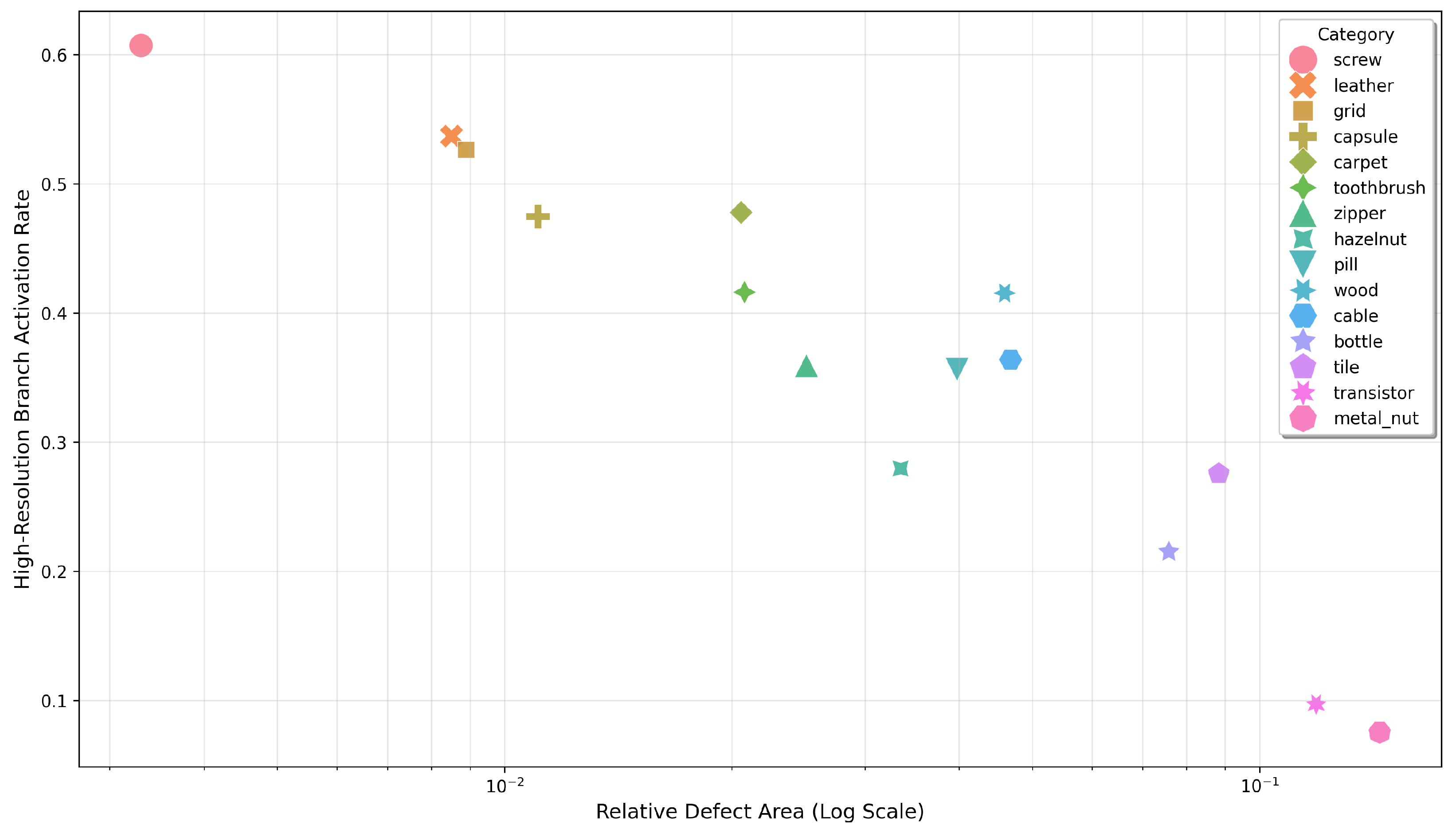
As illustrated in Figure 2, to verify the efficacy of the resolution decision module, we extracted all ground-truth defective samples from the test set and calculated the joint distribution of their relative area and high-resolution branch activation rate under a $224\times 224$ input. The $224\times 224$ resolution was selected as the baseline because it is the standard pre-training input size for current mainstream backbone networks. It represents the model’s fundamental perception capability under conventional computational configurations, providing an accurate reference for measuring when the model requires additional high-resolution resources. In the figure, the horizontal axis denotes the ratio of the defect area to the total image area on a logarithmic scale, while the vertical axis represents the probability of a sample triggering the high-resolution branch during inference. To avoid interference from zero-inflated distributions caused by normal samples, only defective samples are visualized. A significant negative correlation is clearly observed: as the relative area decreases and detection difficulty increases, the bubble positions shift markedly upward. This demonstrates that the model can accurately perceive defect scale and difficulty, dynamically allocating high-resolution computational resources. For large-area defects, such as damaged metal nuts, the model tends to rely on the low-resolution branch to conserve resources. Conversely, for tiny defects, the model is compelled to activate the high-resolution branch to capture high-frequency details. Furthermore, comparing different categories at the same relative area level reveals that texture-based categories, such as leather and tile, generally exhibit higher high-resolution branch selection probabilities than structural objects of similar sizes, such as capsules and bottles. This is because texture defects typically manifest as high-frequency signal anomalies, such as fine scratches or color inconsistencies, which are highly susceptible to feature loss due to downsampling at low resolutions. These defects require higher resolutions to effectively distinguish defect signals from background noise. In contrast, structural defects primarily rely on geometric contour information and are relatively less sensitive to resolution. This phenomenon further confirms that the model not only learns the size of defects but also internalizes the detection difficulty priors associated with different material attributes.

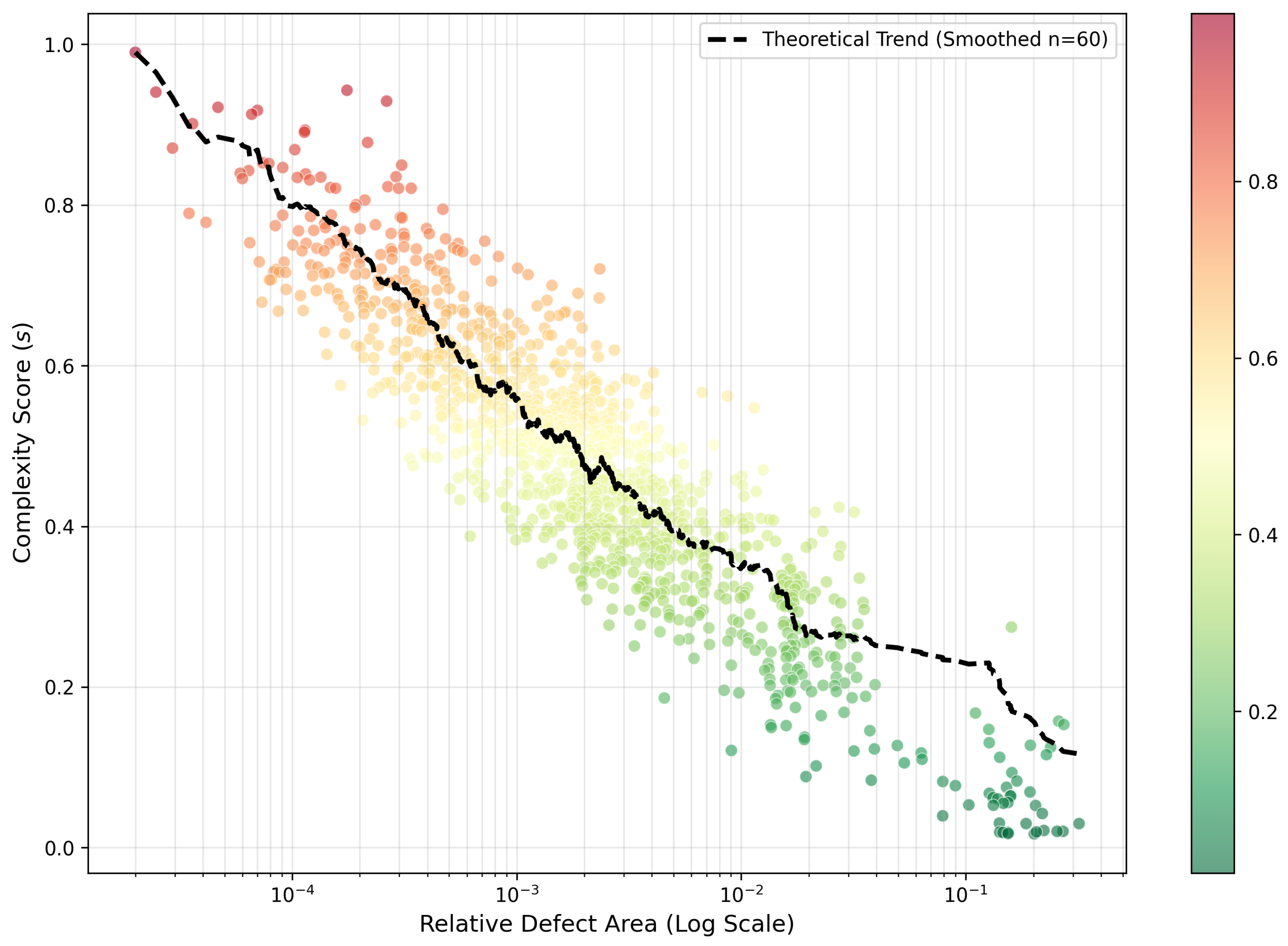
As illustrated in Figure 3, to further validate the model’s adaptive capability in extreme small-defect scenarios and address the limitations of the preceding analysis, we conducted a fine-grained complexity evaluation on all defective test samples from the VisA dataset. Unlike the previous figure, which primarily depicted the average statistical patterns across categories in the MVTec AD dataset, that analysis aimed to reveal the macroscopic correspondence between defect scale and resolution selection via category means. Given that the average defect proportions in MVTec AD span an extensive range from 0.33% to 14.42%, covering a broad spectrum from extremely difficult to trivial cases, the current figure specifically targets the more challenging VisA dataset. Here, the defect proportion is confined to a narrow range between 0.27% and 1.87%, representing a typical collection of high-difficulty minute defects. Consequently, instead of averaging by category, we visualized all defective samples as a unified whole to elucidate the model’s fine-grained perception capability within similarly high-difficulty tasks. In the figure, the horizontal axis represents the ratio of the defect area to the total image area on a logarithmic scale, while the vertical axis denotes the comprehensive complexity score s triggered during inference. This score is derived from a weighted calculation of the high-resolution branch activation rate, feature computational cost, and inference latency, thereby providing a more quantitative reflection of the model’s actual computational resource consumption. A distinct downward trend is clearly observable: as the relative area decreases, the complexity score exhibits a nonlinear increase. This demonstrates that even within the VisA dataset, characterized by its overall minuscule defects, the model remains highly sensitive, effectively distinguishing between extremely small defects (0.27%) and relatively larger ones (1.87%), and allocating significantly higher computational resources to the former. This result not only corroborates the model’s robustness in low signal-to-noise ratio environments but also clarifies that the adaptive mechanism does not rely solely on category priors. Instead, it dynamically adjusts based on the instance-level difficulty of each sample, thereby achieving an optimal allocation of computational resources without compromising detection accuracy.

4.5. Qualitative Comparisons

In this study, GLAD [29] and VLMDiff [25] are selected as the primary baselines for qualitative analysis. Both methods are diffusion-based, sharing high methodological relevance with our approach. GLAD is included due to its superior performance in both anomaly detection and localization tasks, while VLMDiff, as the most recent state-of-the-art method, represents the current frontier with excellent quantitative metrics.

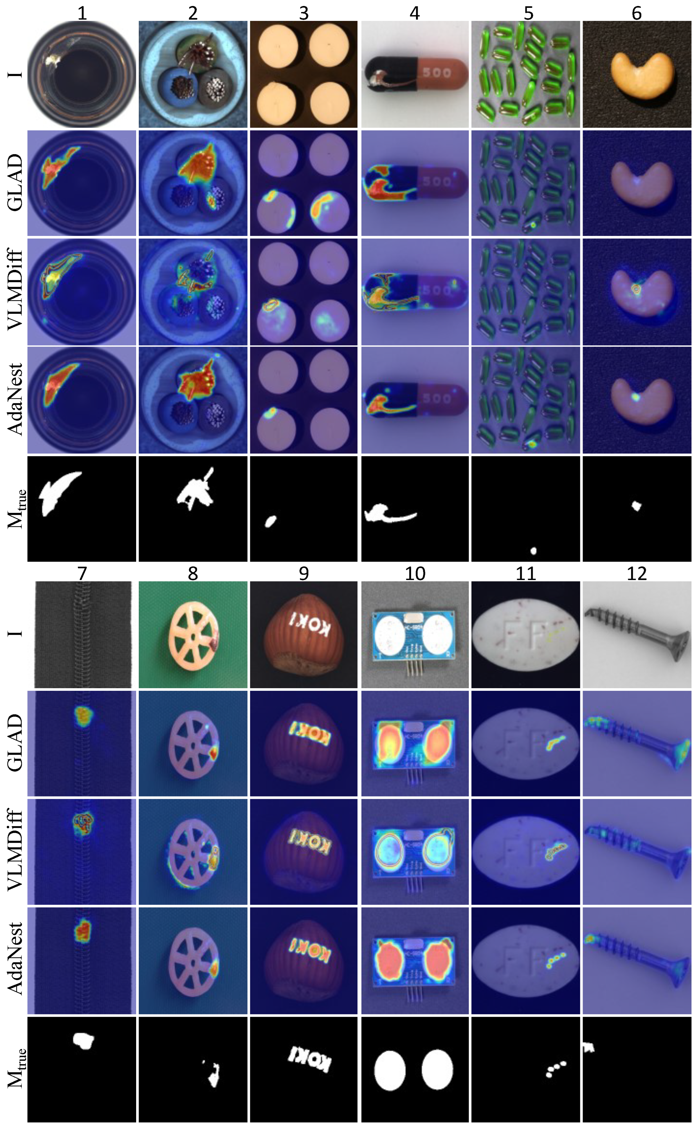
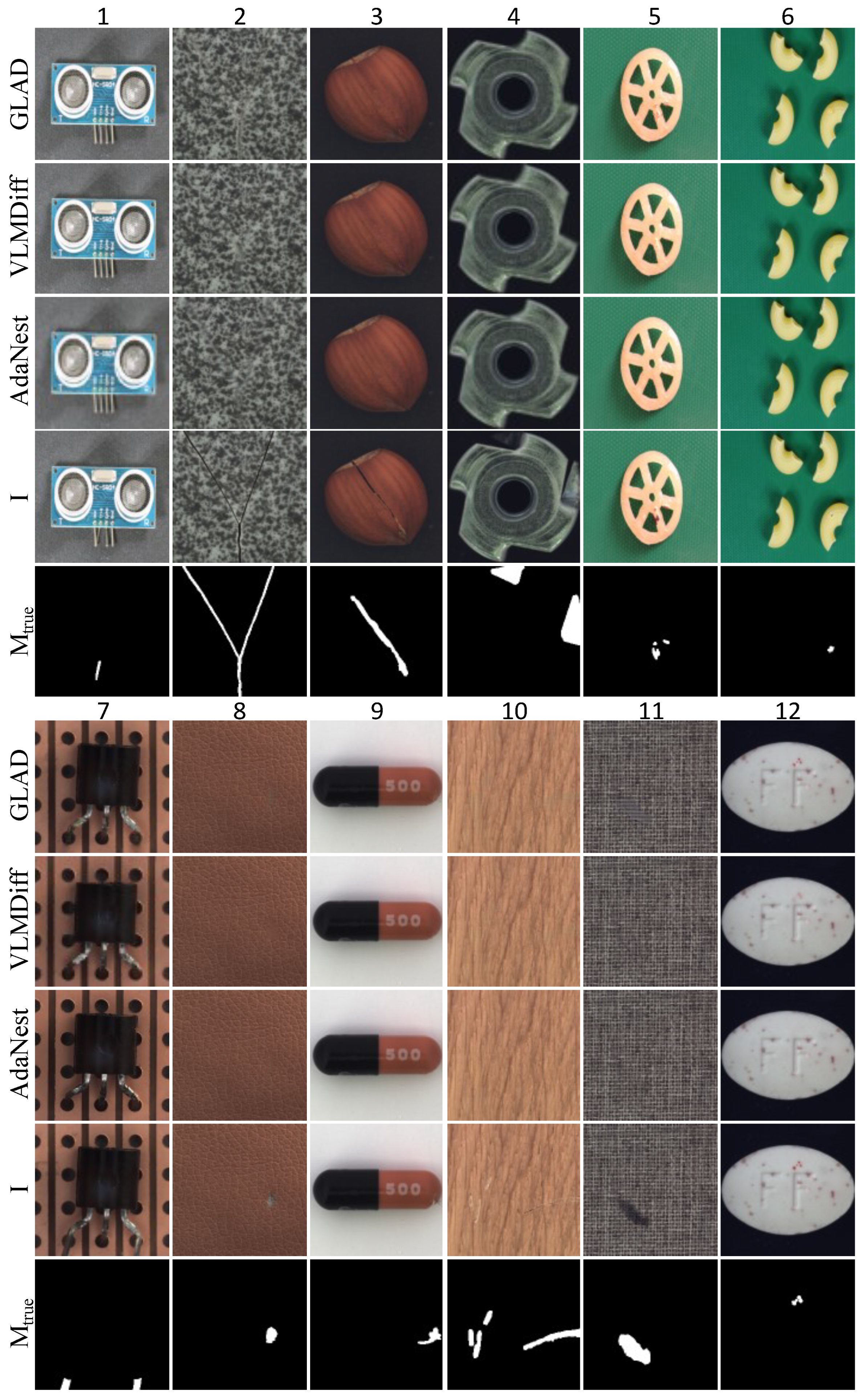
Figure 4 presents a qualitative comparison of AdaNMD against these advanced methods on the MVTec AD and VisA datasets. The first row displays the original anomalous images, the middle three rows show the anomaly heatmaps generated by GLAD, VLMDiff, and AdaNMD, respectively, and the final row provides the ground-truth anomaly masks. Visually, AdaNMD demonstrates more precise and focused anomaly responses across various challenging cases, effectively overcoming the limitations of existing methods.

Specifically, columns 2 and 3 illustrate detection difficulties in complex backgrounds. GLAD exhibits obvious false positives, misidentifying normal textures as anomalies, while VLMDiff yields weak and scattered responses without high-confidence clusters. In contrast, AdaNMD accurately localizes defects while suppressing background noise. In the capsule foreign object scenario (column 4), both GLAD and VLMDiff struggle to distinguish the main body from attached objects, leading to false activations; AdaNMD, however, achieves precise separation. Column 5 highlights a severe miss by VLMDiff on a tiny target, whereas AdaNMD clearly outlines the anomaly. Column 6 further validates model sensitivity: GLAD shows low confidence, and VLMDiff suffers from over-localization with blurry boundaries, while AdaNMD precisely highlights fine-grained anomalies.

For structural defects, column 7 demonstrates zipper tooth missing detection. AdaNMD generates continuous anomaly maps with sharp boundaries, significantly outperforming the discrete or diffuse responses of the baselines by fully outlining the missing teeth. In high-texture interference scenarios, such as the missing solder joint on a PCB (column 10), GLAD and VLMDiff are prone to false positives caused by dense traces. AdaNMD successfully focuses on the true missing location, showing superior anti-interference capability. Finally, column 12 illustrates complex damage on screw heads, where AdaNMD accurately identifies fractures and wear at the thread root, with the heatmap distribution closely matching the physical damage morphology. Collectively, these results confirm AdaNMD’s superior robustness and localization precision.

Figure 5 presents a qualitative comparison of the reconstruction results between AdaNMD and current mainstream baseline methods. From top to bottom, the figure displays the reconstructed images generated by GLAD and VLMDiff, the results of AdaNMD, the original anomalous images, and the ground-truth anomaly masks. By observing samples across different categories, it is evident that AdaNMD possesses distinct advantages in texture preservation and structural restoration.

Specifically, in column 2, GLAD and VLMDiff exhibit noticeable blurring or artifacts when reconstructing surface cracks on tiles, failing to effectively “erase” the defects. In contrast, AdaNMD accurately restores the smoothness and edge sharpness of the cracked regions while preserving the glossy texture of the surrounding glaze. Column 3 illustrates the repair of fissures on nut surfaces. After processing by GLAD and VLMDiff, unnatural texture connections and visible repair traces remain in the defective areas, whereas the surface generated by AdaNMD appears seamless and integral. In food scenarios involving complex geometries (columns 5 and 6), GLAD and VLMDiff suffer from severe distortions when repairing dents or fractures on curved surfaces, manifesting as morphological swelling or texture misalignment. This indicates that the defects are not completely eliminated and new geometric distortions are introduced. Conversely, AdaNMD maintains the natural curvature and material consistency of the objects. In column 8, the leather texture reconstructed by GLAD appears slightly rigid, destroying its original organic feel. AdaNMD, however, naturally continues the grain direction and light-shadow transitions, leaving virtually no visible traces of repair. For materials with high texture consistency, VLMDiff introduces a slight color shift in the repaired wood grain (column 10), resulting in texture discontinuity. AdaNMD precisely recovers the natural texture and color continuity of the wood. Column 9 shows that VLMDiff fails to completely remove the defects in the pill spot area, leaving obvious artifacts. In column 11, GLAD distorts the orientation of the fabric fibers, whereas AdaNMD effectively maintains the texture direction, ensuring the authentic restoration of the fabric pattern. Finally, in column 12, neither GLAD nor VLMDiff can effectively repair the surface damage on the pills, leaving the defects still visible. This further highlights the superior performance of AdaNMD in repairing minute flaws. In summary, AdaNMD significantly outperforms the baseline methods in reconstruction quality, capable of generating cleaner and more physically plausible normal sample images.

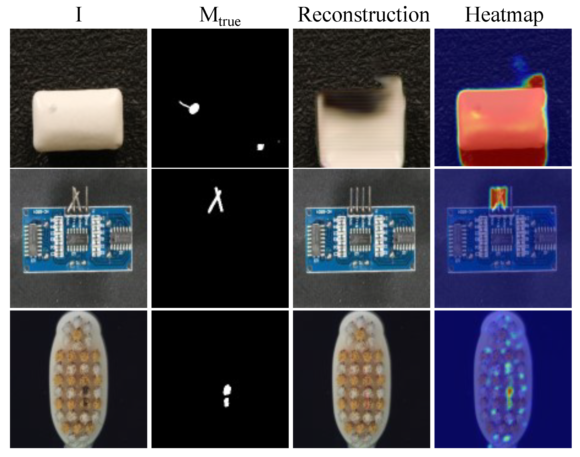
Despite the superior performance of AdaNMD in most scenarios, it still exhibits certain limitations when facing specific types of extreme defects. As illustrated in Figure 6, we present typical failure cases on the VisA and MVTec AD datasets.

First, in the Chewinggum category of the VisA dataset (first row), when confronted with large-area missing and deformation defects at the object edges, the model fails to accurately reconstruct the damaged regions. Instead, it causes texture loss in normal areas and an overall downward shift in the global structure, leading to severe false positives where the heatmap localization range significantly exceeds the actual ground-truth mask. The primary cause is the deviation of the adaptive mechanism in the resolution decision module when handling complex geometric deformations. When the input image contains significant structural defects, the decision module may incorrectly evaluate the image complexity, activating the medium-to-low resolution branches that possess larger receptive fields but retain fewer spatial details. Although these branches can capture global semantics, they struggle to maintain pixel-level precise alignment, resulting in geometric shifts in the reconstructed images. Furthermore, AdaGN normalization relies excessively on the global statistical information of timestep embeddings when modulating features, which further exacerbates the blurring of local texture generation and causes severe artifacts during differential localization.

Second, in the PCB2 category of the VisA dataset (second row), the model demonstrates a tendency toward over-repair for twisted sensor probes. The reconstructed image not only repairs the anomalous region but also forcefully corrects the structurally distorted probe back to a normal morphology. Consequently, during the differential comparison, the twisted part in the original image and the normal part in the reconstructed image jointly form a high-response region, causing the final localization result to include non-defective structural differences.

Finally, in the Toothbrush category of the MVTec AD dataset (third row), when facing extremely tiny point-like defects, the model maintains extremely high clarity in reconstructing the bristle texture, but simultaneously generates numerous fragmented noise-like false detections at the non-defective bristle tips. This is also attributed to the imbalanced sensitivity of the resolution decision module to high-frequency texture regions. Toothbrush bristles represent typical high-frequency complex textures. To preserve these fine structures, the decision module tends to select the high-resolution branch or a hybrid path. However, in such an extremely high-frequency background, the cross-scale self-distillation mechanism may exhibit subtle alignment errors when transmitting the strong semantic constraints of the teacher model. As a result, while striving to restore the bristle details, the model misjudges normal texture fluctuations as anomalous signals, forming discrete spot-like noise in the heatmap.

4.6. Ablation Study

As shown in

Table 5. Results of the ablation study. Detection results are reported in AUROC and localization results are reported in AUPRO.

Group	Condition	VisA		MVTec AD
		Det.	Loc.	Det.	Loc.
Component	w/o Nested Diffusion	−0.6	−1.3	−0.8	−1.7
	w/o Feature Fusion	−0.3	−0.4	−0.2	−0.1
	w/o Resolution Decision	−0.1	−0.2	−0.1	+0.3
Loss function	w/o ${\mathcal{L}}_{ϵ}^{distill}$	−1.8	−2.5	−1.9	−2.5
	w/o ${\mathcal{L}}_{\mu }^{distill}$	−0.8	−1.2	−0.7	−1.4
	w/o ${\mathcal{L}}_M^{distill}$	−0.7	−1.3	−0.9	−1.7
	w/o ${\mathcal{L}}_{eff}$	−0.1	+0.1	−0.2	−0.3
	w/o ${\mathcal{L}}_{conf}$	−0.1	−0.3	−0.2	−0.5
	w/o ${\mathcal{L}}_{bal}$	−0.9	−1.4	−1.5	−2.2
Target Distribution	$q=[0.5,0.3,0.2]$	−1.3	−1.7	−0.5	−1.0
	$q=[0.33,0.33,0.34]$	−0.4	−0.6	−0.3	−0.4
Diffusion step num	5 steps	−1.1	−4.2	−0.8	−1.4
	10 steps	−0.6	−1.3	−0.6	−1.1
	50 steps	−0.2	+0.1	−0.7	−0.4
AdaNMD	Triple-layer, 20 steps, $q=[0.2,0.3,0.5]$	98.6	95	99.1	94.4

, to validate the effectiveness of the proposed nested diffusion architecture, this study constructs a structurally aligned U-Net baseline for ablation analysis. This baseline adopts a standard encoder-decoder structure with four levels of downsampling, where feature map resolution is halved and channel count doubled at each stage, and a symmetric decoder with four upsampling levels to restore resolution. To ensure a fair comparison, the output resolutions of the last three upsampling layers in this U-Net are adjusted to match those of AdaNMD low, mid, and high resolution decoding branches respectively. The outputs from the last three downsampling stages are denoted as $F_1$, $F_2$, $F_3$ and fed into the same FPN feature fusion module. All other components, including the resolution decision module and the full set of loss functions, remain unchanged. Under this setting, removing the nested multi-resolution collaborative denoising mechanism leads to a significant performance drop. On VisA, AUROC decreases by 0.6% and AUPRO declines by 1.3%. On MVTec AD, AUROC drops by 0.8% and AUPRO falls by 1.7%. These results strongly indicate that AdaNMD coarse-to-fine, cross-scale feedback nested structure effectively promotes joint optimization of global semantic consistency and local anomalous details.

To evaluate the role of the FPN feature fusion module, this study bypasses the feature fusion step within the complete AdaNMD framework by directly feeding the raw multi-scale encoder features $F_1$, $F_2$, $F_3$ into subsequent stages in place of the fused pyramid representations $P_1$, $P_2$, $P_3$, while keeping all other components unchanged. Experimental results show that this modification leads to an AUROC drop of 0.3% and an AUPRO decline of 0.4% on VisA, and an AUROC reduction of 0.2% and an AUPRO decrease of 0.1% on MVTec AD. Although the performance degradation is relatively modest, this result confirms that the FPN feature fusion module, through top-down semantic enhancement and cross-level feature aggregation, effectively improves spatial consistency and contextual awareness in multi-scale representations, thereby providing a more robust feature foundation for subsequent decoding and decision making.

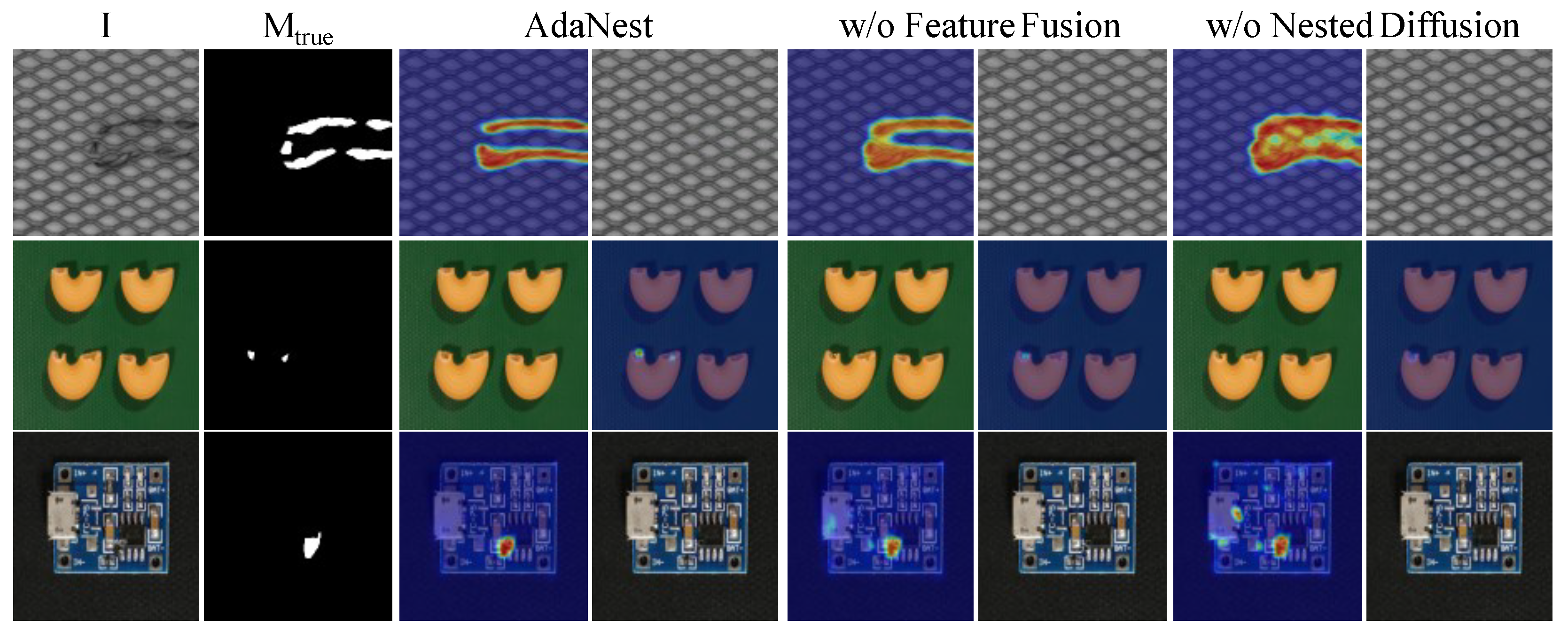
Figure 7 presents a qualitative comparison of the proposed nested diffusion model combined with the Feature Pyramid Network (FPN) against two variant methods across different industrial defect scenarios. The figure consists of three rows and eight columns. The first row displays samples with irregular texture defects from the Grid category of the MVTec AD dataset; the second row shows tiny defect samples from the Macaroni1 category of the VisA dataset; and the third row illustrates complex structural defects from the PCB4 category of the VisA dataset. For each row, the first column shows the original anomalous images, and the second column provides the corresponding ground-truth anomaly masks. Columns 3 and 4 display the localization heatmaps and reconstruction results of our full model, respectively. Columns 5 and 6 present the heatmaps and reconstruction results of the nested diffusion model without FPN, while columns 7 and 8 show those of the single-layer diffusion model combined with FPN.

In the first row, addressing irregular texture defects, the heatmap generated by our model precisely focuses on the defect region with sharp edges, and the reconstruction achieves pixel-level seamless integration of the grid texture. This is attributed to the FPN providing high-resolution shallow features to align the grid lines, while the nested diffusion structure utilizes deep semantics to perfectly infer the geometric structure of the missing parts. In contrast, although the model without FPN achieves relatively concentrated localization, its heatmap edges exhibit jaggedness, and the reconstructed grid lines show fractures and misalignment. This is because the lack of lateral connections causes high-level features to lose precise spatial location information during downsampling, making pixel-level alignment unachievable during upsampling recovery. The single-layer diffusion model with FPN, however, suffers from an excessively large activation range accompanied by obvious background noise, and the reconstructed region appears as an over-smoothed blurry shadow. The reason is that the single-layer model lacks hierarchical generative reasoning capability, making it difficult to distinguish high-frequency differences between defects and normal textures in complex backgrounds, thus tending to generate probabilistically averaged results.

In the second row, targeting tiny defects, our model successfully and precisely activates two minute defects with extremely high confidence. The reconstruction exhibits clear details and natural color transitions, reflecting the dual advantages of multi-scale feature fusion and hierarchical semantic guidance. The model without FPN can only detect the larger of the two defects, with the other tiny target almost missed. Moreover, the reconstructed defect edges are blurry and the texture is discontinuous, indicating that deep features suffer a significant reduction in spatial resolution after multiple downsampling operations, leading to the erasure of physical information of extremely small targets. The single-layer diffusion model with FPN performs the worst; it not only misses one defect but also yields an extremely weak response for the remaining one, with severely distorted reconstruction. This demonstrates that even with multi-scale inputs, the single-layer model still lacks the coarse-to-fine progressive reasoning capability required to amplify weak anomalous signals.

In the third row, focusing on complex structural defects in the PCB4 category, our model forms a highly concentrated activation region at the true defect location with sharp boundaries and no false positives. In the reconstructed image, component edges are crisp, and the transitions between solder joints and traces are natural, proving its ability to precisely locate minute anomalies and restore high-frequency details in complex circuit board backgrounds. Although the model without FPN responds at the original location, it exhibits a diffuse activation halo around it, and the reconstruction shows obvious stripe-like fractures. This is a typical manifestation of localization drift and texture segmentation caused by spatial resolution loss. The single-layer diffusion model with FPN generates large-area false positives in non-defective regions accompanied by scattered pseudo-activations, and the core reconstruction is significantly blurred. This reflects its inability to effectively distinguish true anomalies from texture noise such as dense solder joints, demonstrating the weakest robustness and anti-interference capability among the compared methods.

To further examine the necessity of the resolution decision module, this study fixes inference to use only the high-resolution branch output, effectively disabling the dynamic routing mechanism while preserving all other training and architectural settings. Surprisingly, this strategy yields slight AUPRO improvements of +0.1% on VisA and +0.3% on MVTec AD, confirming that the high-resolution path inherently possesses the strongest representational capacity. However, this approach completely loses computational flexibility, resulting in more than a two-fold slowdown in inference speed. In contrast, the proposed dynamic decision mechanism achieves on-demand computation with nearly no loss in localization accuracy, demonstrating the practical value of co-designing efficiency and precision, particularly beneficial for resource-constrained industrial deployment scenarios.

Given that TransFusion [27] has already conducted a systematic ablation of the individual sub-losses within multi-scale supervision for industrial anomaly detection, this work does not repeat validation of these established components. Instead, this study focuses on two newly introduced loss mechanisms, multi-task self-distillation loss and dynamic routing auxiliary loss, whose constituent sub-losses are all applied for the first time to industrial image anomaly detection.

Ablation studies are performed on the three sub-losses of the multi-task self-distillation loss to systematically assess their roles in cross-scale knowledge transfer. First, removing the noise distillation sub-loss ${\mathcal{L}}_{ϵ}^{distill}$ results in a 2.5% drop in AUPRO on both VisA and MVTec AD. This significant degradation indicates that the reconstruction uncertainty modeled by the high-resolution branch during denoising, for instance, the confidence distribution over anomalous pixels, effectively guides lightweight branches in distinguishing normal from anomalous patterns, which is especially critical in fine-grained anomaly scenarios. Second, ablating the feature mean distillation sub-loss ${\mathcal{L}}_{\mu }^{distill}$ leads to a 1.2% AUPRO decrease on VisA and a 1.4% drop on MVTec AD. This demonstrates that aligning channel-wise feature means of mid- and low-resolution branches with those of the high-resolution branch effectively mitigates semantic shifts caused by resolution differences, thereby enhancing cross-scale representation consistency. Finally, removing the mask distillation sub-loss ${\mathcal{L}}_m^{distill}$ causes AUPRO to decline by 1.3% on VisA and 1.7% on MVTec AD. This confirms that using the spatial anomaly response generated by the high-resolution branch as a soft supervision signal significantly strengthens the sensitivity of lightweight branches to anomalous boundaries.

To systematically evaluate the impact of each sub-component in the dynamic routing auxiliary loss on model performance and inference efficiency, this study conducts ablation experiments by removing the efficiency loss ${\mathcal{L}}_{eff}$, confidence loss ${\mathcal{L}}_{conf}$, and load-balancing loss ${\mathcal{L}}_{bal}$ individually. Removing the efficiency loss ${\mathcal{L}}_{eff}$ eliminates explicit consideration of computational costs across decoding paths during training. As a result, the high-resolution branch, due to its stronger reconstruction capability, achieves lower values under the main supervision loss, causing the routing module to gradually favor this branch exclusively in later training stages. Although this strategy yields a slight AUPRO improvement of +0.1% on VisA, it leads to a 0.3% drop on MVTec AD and increases average inference time from 0.49 s to 0.60 s, significantly slower than the original model. This indicates that while partial localization capability is retained, the core advantage of on-demand computation is entirely lost, resulting in substantially degraded inference efficiency. When the confidence loss ${\mathcal{L}}_{conf}$ is removed, the model exhibits higher decision uncertainty on samples near the medium-complexity boundary. Minor input perturbations can cause abrupt switches in routing decisions across branches, introducing inference instability. This issue is particularly critical in industrial settings, where real-world images often suffer from illumination variations or slight occlusions. Experimental results show AUPRO declines of 0.3% on VisA and 0.5% on MVTec AD, with inference time rising to 0.52s, confirming that the absence of confidence guidance undermines robustness and deployment reliability. Finally, ablating the load-balancing loss ${\mathcal{L}}_{bal}$ causes the routing module to collapse toward a single frequently used path, typically the low-resolution branch, since most samples in industrial datasets belong to simple categories. Consequently, the high-resolution branch is activated only on rare extreme cases and fails to receive sufficient training. This training imbalance severely impairs generalization to complex anomalies, leading to a sharp performance drop. AUPRO decreases by 1.4% on VisA and 2.2% on MVTec AD. Although inference time slightly improves to 0.46s, this gain comes at the cost of critical task performance, underscoring the essential role of load balancing in sustaining the effectiveness of the multi-scale architecture.

Regarding the auxiliary loss weights, we follow an empirical rule to scale each auxiliary loss term to 10%–20% of the primary loss. This ratio provides effective gradient supplementation without interfering with the learning of the backbone network. Consequently, the auxiliary loss weights in Section 3.4.2 and Section 3.4.3 are excluded from the ablation variables. To investigate the impact of the target activation frequency distribution q on model performance and to validate the rationality of the current configuration $[0.2,0.3,0.5]$, we designed an ablation study by adjusting q to a uniform distribution $[0.33,0.33,0.34]$ and a low-complexity-biased distribution $[0.5,0.3,0.2]$ for comparison. For the low-complexity-biased distribution, the thresholds are set to ${\tau }_1=0.5$ and ${\tau }_2=0.8$. For the uniform distribution, the thresholds are set to ${\tau }_1=0.33$ and ${\tau }_2=0.66$. For the proposed configuration, the thresholds are set to ${\tau }_1=0.2$ and ${\tau }_2=0.5$. The experimental results indicate that altering the distribution configuration leads to varying degrees of performance degradation. Specifically, the low-complexity-biased distribution ($q=[0.5,0.3,0.2]$) yields the most significant performance drop, while the uniform distribution ($q=[0.33,0.33,0.34]$) exhibits a relatively smaller decline. This phenomenon can be attributed to the fact that the sample complexity in anomaly detection tasks typically follows a long-tailed distribution, where simple or medium-complexity samples constitute the majority, whereas high-complexity hard cases are scarce but crucial. Enforcing a uniform distribution wastes computational resources on simple samples, while excessively biasing towards low complexity weakens the high-resolution branch’s capability to parse challenging defects.

Table 6. Efficiency and computational complexity evaluation of the AdaNMD Framework.

Module/Path	Params	FLOPs	Latency	GPU Mem.
	[$\times {10}^4$]	[$\times {10}^6$]	[ms]	[MB]
Feature Extraction	1315.2	6354.9	5.6	-
Feature Fusion	28.8	344.8	2.1	-
Resolution Decision	0.7	0.9	0.9	-
Decoder 1	1153.9	2685.4	1.9	-
Decoder 2	2237.3	8593.3	3.3	-
Decoder 3	560.0	8608.9	5.3	-
Decoder 4	135.5	12,690.0	11.7	-
Low-resolution path	4736.0	17,979.3	13.7	625.91
Medium-resolution path	5296.0	26,588.2	19.0	968.75
High-resolution path	5431.4	39,278.2	30.8	1274.52

provides a detailed breakdown of the computational complexity and inference latency of our proposed model. Specifically, Decoder 1 through Decoder 4 correspond to the four components arranged from left to right within the Nested Decoder shown in Figure 1. First, the Resolution Decision module exhibits extremely low parameter count, FLOPs, and latency. This perfectly aligns with our design philosophy. the routing decision mechanism should be as lightweight as possible to perform path selection with minimal overhead, thereby avoiding the occupation of inference resources from the encoder and decoder. Second, in terms of parameter count, Decoder 1 and Decoder 2 dominate, which is primarily attributed to the integration of self-attention mechanisms within them. In contrast, regarding FLOPs, the values for Decoder 3 and Decoder 4 are significantly higher than those of the former two. This is because FLOPs depend not only on the number of channels but are also highly sensitive to the spatial resolution of the feature maps. Since Decoder 3 and Decoder 4 process high-resolution features, their computational costs increase dramatically. Out of consideration for computational overhead and memory footprint, we intentionally omitted the attention mechanism at these high-resolution levels to prevent GPU memory overflow. Furthermore, to evaluate the practical deployment potential of the model in industrial environments, we specifically analyzed the GPU memory usage across the three paths with different resolutions. The analysis reveals a significant positive correlation between resource consumption and path resolution; that is, as the path resolution increases, the model’s parameter count, FLOPs, inference latency, and GPU memory usage all increase substantially. Finally, it should be noted that the inference latency reported in Table 6 is measured per single diffusion time step. The actual inference time requires multiplying this value by the total number of diffusion steps. Therefore, the data in Table 6 and

Table 7. The average inference time for processing a single sample using one NVIDIA RTX A4000 GPU, reported in seconds. Here, l, m, and h denote the low-resolution, medium-resolution, and high-resolution decoder branches, respectively.

AdaNMD Variants		Comparison Methods
Method	Time [s]	Method	Time [s]
AdaNMD	0.49	DiffAD [24]	1.95
w/o ${\mathcal{L}}_{eff}$	0.60	GLAD [29]	1.35
w/o ${\mathcal{L}}_{conf}$	0.52	TransFusion [27]	0.90
w/o ${\mathcal{L}}_{bal}$	0.46	LASB [28]	0.56
Only h	0.62	InvAD [26]	0.11
Only m	0.47	VLMDiff [25]	2.10
Only l	0.36

do not conflict but rather complement each other.

As shown in Table 7, the proposed nested diffusion architecture significantly reduces overall computational cost through multi-resolution collaborative modeling. AdaNMD achieves an excellent balance between accuracy and speed for industrial applications by enabling efficient on-demand computation via its nested structure and dynamic routing, all while maintaining high detection performance. Notably, InvAD obtains a substantial improvement in inference speed by utilizing only 3 diffusion steps. Consequently, this study systematically evaluates the impact of the number of diffusion steps T on detection performance. When $T=5$, AUPRO drops by 4.2% on VisA and 1.4% on MVTec AD, indicating that an extremely short denoising process fails to adequately recover anomalous details, particularly in low-contrast scenarios such as pill spots, where reconstructions become overly smooth. When $T=10$, AUPRO decreases by 1.3% on VisA and 1.1% on MVTec AD. Although performance partially recovers, it remains notably below that of the default setting. In contrast, when $T=50$, AUPRO on VisA improves marginally by 0.1%, but AUPRO on MVTec AD declines by 0.4%, accompanied by a significant increase in inference time. This non-monotonic trend suggests that an excessively long diffusion process not only yields diminishing returns but may also reduce sensitivity to anomalies due to over-optimization of normal-region textures. Taking localization accuracy, robustness, and computational efficiency into account, $T=20$ is identified as the optimal trade-off for industrial deployment.

5. Conclusions

Addressing the inherent dilemma between multi-scale modeling capability and computational efficiency in diffusion models for industrial anomaly detection, this paper proposes a novel nested adaptive multi-resolution diffusion model named AdaNMD. By constructing a three-way nested decoding architecture that is fully activated during training and dynamically selected during inference and by integrating AdaGN normalization, an improved FPN module, and a cross-scale self-distillation mechanism, this study successfully establishes an input-adaptive efficient inference paradigm. Extensive experiments on the VisA and MVTec AD datasets demonstrate that AdaNMD achieves a state-of-the-art average AUPRO of 94.7% and improves inference speed by approximately 21% while maintaining almost lossless localization accuracy. These results strongly prove that the proposed method can significantly reduce redundant computations while ensuring pixel-level detection precision, thereby providing a viable path for deploying diffusion models on resource-constrained edge devices. Although AdaNMD exhibits superior performance in most scenarios, it still presents certain limitations when facing specific extreme defects, including reconstruction shifts caused by geometric deformations, structural over-repair, and false detections in high-frequency textures.

Future research will focus on exploring effective implementation paths to address the aforementioned limitations. Specifically, we plan to introduce local attention mechanisms or spatially variant normalization strategies to overcome the reliance on global statistics. By enabling the model to perceive local spatial variations, such approaches can facilitate adaptive feature calibration in complex deformation regions, thereby alleviating reconstruction biases caused by global smoothing effects. On this basis, we will further explore how to incorporate complex geometric constraints to optimize the complexity evaluation logic while maintaining the lightweight nature of dynamic routing, and investigate refining semantic alignment mechanisms for high-frequency textures in the absence of semantic labels. Furthermore, we aim to conduct extensive deployment verification and memory optimization on resource-constrained edge hardware, striving to expand the applicability of this method in real-world industrial scenarios by tackling these non-trivial open problems.

References

1. Zhang, H.; Wang, Z.; Zeng, D.; Wu, Z.; Jiang, Y.G. DiffusionAD: Norm-guided one-step denoising diffusion for anomaly detection. IEEE Trans. Pattern Anal. Mach. Intell. 2025, 47, 7140–7152. [Google Scholar] [CrossRef] [Scilit]
2. Han, J.; Feng, S.; Zhou, M.; Zhang, X.; Ong, Y.S.; Li, X. Diffusion model in normal gathering latent space for time series anomaly detection. In Proceedings of the Joint European Conference on Machine Learning and Knowledge Discovery in Databases; Springer: Berlin/Heidelberg, Germany, 2024; pp. 284–300. [Google Scholar]
3. Zhang, F.; Pilanci, M. Analyzing neural network-based generative diffusion models through convex optimization. arXiv 2024, arXiv:2402.01965. [Google Scholar]
4. Zhu, A.; Wang, W.; Yan, C. Flow-guided diffusion autoencoder for unsupervised video anomaly detection. In Proceedings of the Chinese Conference on Pattern Recognition and Computer Vision (PRCV); Springer: Berlin/Heidelberg, Germany, 2023; pp. 183–194. [Google Scholar]
5. Luo, W. A comprehensive survey on knowledge distillation of diffusion models. arXiv 2023, arXiv:2304.04262. [Google Scholar]
6. Chen, J.; Zhang, A.; Li, M.; Smola, A.; Yang, D. A cheaper and better diffusion language model with soft-masked noise. In Proceedings of the 2023 Conference on Empirical Methods in Natural Language Processing; Association for Computational Linguistics: Stroudsburg, PA, USA, 2023; pp. 4765–4775. [Google Scholar]
7. Hang, T.; Gu, S.; Bao, J.; Wei, F.; Chen, D.; Geng, X.; Guo, B. Improved noise schedule for diffusion training. In Proceedings of the IEEE/CVF International Conference on Computer Vision; IEEE: New York, NY, USA, 2025; pp. 4796–4806. [Google Scholar]
8. Rombach, R.; Blattmann, A.; Lorenz, D.; Esser, P.; Ommer, B. High-resolution image synthesis with latent diffusion models. In Proceedings of the IEEE/CVF Conference on Computer Vision and Pattern Recognition; IEEE: New York, NY, USA, 2022; pp. 10684–10695. [Google Scholar]
9. Shang, Y.; Yuan, Z.; Xie, B.; Wu, B.; Yan, Y. Post-training quantization on diffusion models. In Proceedings of the IEEE/CVF Conference on Computer Vision and Pattern Recognition; IEEE: New York, NY, USA, 2023; pp. 1972–1981. [Google Scholar]
10. Zou, Y.; Jeong, J.; Pemula, L.; Zhang, D.; Dabeer, O. Spot-the-difference self-supervised pre-training for anomaly detection and segmentation. In Proceedings of the European Conference on Computer Vision; Springer: Berlin/Heidelberg, Germany, 2022; pp. 392–408. [Google Scholar]
11. Bergmann, P.; Batzner, K.; Fauser, M.; Sattlegger, D.; Steger, C. The MVTec anomaly detection dataset: A comprehensive real-world dataset for unsupervised anomaly detection. Int. J. Comput. Vis. 2021, 129, 1038–1059. [Google Scholar] [CrossRef] [Scilit]
12. Bercea, C.I.; Neumayr, M.; Rueckert, D.; Schnabel, J.A. Mask, stitch, and re-sample: Enhancing robustness and generalizability in anomaly detection through automatic diffusion models. arXiv 2023, arXiv:2305.19643. [Google Scholar]
13. Hu, X.; Jin, C. AnoDODE: Anomaly detection with diffusion ODE. arXiv 2023, arXiv:2310.06420. [Google Scholar]
14. Wang, H.; Dai, L.; Tong, J.; Zhai, Y. Odd: One-class anomaly detection via the diffusion model. In Proceedings of the 2023 IEEE International Conference on Image Processing (ICIP); IEEE: New York, NY, USA, 2023; pp. 3000–3004. [Google Scholar]
15. Le Lan, C.; Dinh, L. Perfect density models cannot guarantee anomaly detection. Entropy 2021, 23, 1690. [Google Scholar] [CrossRef] [Scilit]
16. Wang, W.; Xu, Y.; Feng, F.; Lin, X.; He, X.; Chua, T.S. Diffusion recommender model. In Proceedings of the 46th International ACM SIGIR Conference on Research and Development in Information Retrieval; Association for Computing Machinery: New York, NY, USA, 2023; pp. 832–841. [Google Scholar]
17. Zhan, J.; Lai, J.; Gao, B.B.; Liu, J.; Chen, X.; Wang, C. Enhancing multi-class anomaly detection via diffusion refinement with dual conditioning. arXiv 2024, arXiv:2407.01905. [Google Scholar]
18. Xu, H.; Xu, S.; Yang, W. Unsupervised industrial anomaly detection with diffusion models. J. Vis. Commun. Image Represent. 2023, 97, 103983. [Google Scholar] [CrossRef] [Scilit]
19. Wu, D.; Fan, S.; Zhou, X.; Yu, L.; Deng, Y.; Zou, J.; Lin, B. Unsupervised anomaly detection via masked diffusion posterior sampling. arXiv 2024, arXiv:2404.17900. [Google Scholar]
20. Wang, B.; Vastola, J.J. The hidden linear structure in score-based models and its application. arXiv 2023, arXiv:2311.10892. [Google Scholar]
21. Han, Y.; Razaviyayn, M.; Xu, R. Neural network-based score estimation in diffusion models: Optimization and generalization. arXiv 2024, arXiv:2401.15604. [Google Scholar]
22. Deveney, T.; Stanczuk, J.; Kreusser, L.; Budd, C.; Schönlieb, C.B. Closing the ODE–SDE gap in score-based diffusion models through the Fokker–Planck equation. Philos. Trans. R. Soc. A Math. Phys. Eng. Sci. 2025, 383. [Google Scholar] [CrossRef] [Scilit]
23. Livernoche, V.; Jain, V.; Hezaveh, Y.; Ravanbakhsh, S. On diffusion modeling for anomaly detection. arXiv 2023, arXiv:2305.18593. [Google Scholar]
24. Zhang, X.; Li, N.; Li, J.; Dai, T.; Jiang, Y.; Xia, S.T. Unsupervised surface anomaly detection with diffusion probabilistic model. In Proceedings of the IEEE/CVF International Conference on Computer Vision; IEEE: New York, NY, USA, 2023; pp. 6782–6791. [Google Scholar]
25. Hicsonmez, S.; El Rahman Shabayek, A.; Aouada, D. VLMDiff: Leveraging Vision-Language Models for Multi-Class Anomaly Detection with Diffusion. In Proceedings of the IEEE/CVF Winter Conference on Applications of Computer Vision; IEEE: New York, NY, USA, 2026; pp. 6309–6319. [Google Scholar]
26. Sakai, S.; He, X.; Gu, C.; Sigal, L.; Hasegawa, T. Invad: Inversion-based reconstruction-free anomaly detection with diffusion models. In Proceedings of the IEEE/CVF Conference on Computer Vision and Pattern Recognition; IEEE: New York, NY, USA, 2026; pp. 21389–21398. [Google Scholar]
27. Fučka, M.; Zavrtanik, V.; Skočaj, D. Transfusion–a transparency-based diffusion model for anomaly detection. In Proceedings of the European Conference on Computer Vision; Springer: Berlin/Heidelberg, Germany, 2024; pp. 91–108. [Google Scholar]
28. Akshay, S.; Narasimhan, N.L.; George, J.; Balasubramanian, V.N. A unified latent schrodinger bridge diffusion model for unsupervised anomaly detection and localization. In Proceedings of the Computer Vision and Pattern Recognition Conference; IEEE: New York, NY, USA, 2025; pp. 25528–25538. [Google Scholar]
29. Yao, H.; Liu, M.; Yin, Z.; Yan, Z.; Hong, X.; Zuo, W. Glad: Towards better reconstruction with global and local adaptive diffusion models for unsupervised anomaly detection. In Proceedings of the European Conference on Computer Vision; Springer: Cham, Switzerland, 2024; pp. 1–17. [Google Scholar]
30. Lu, G.; Zhang, W.; Wang, Z. Optimizing depthwise separable convolution operations on gpus. IEEE Trans. Parallel Distrib. Syst. 2021, 33, 70–87. [Google Scholar] [CrossRef] [Scilit]
31. Wu, Y.; He, K. Group normalization. In Proceedings of the European Conference on Computer Vision (ECCV); Springer: Berlin/Heidelberg, Germany, 2018; pp. 3–19. [Google Scholar]
32. Zhu, L.; Lee, F.; Cai, J.; Yu, H.; Chen, Q. An improved feature pyramid network for object detection. Neurocomputing 2022, 483, 127–139. [Google Scholar] [CrossRef] [Scilit]
33. Jang, J.G.; Quan, C.; Lee, H.D.; Kang, U. Falcon: Lightweight and accurate convolution based on depthwise separable convolution. Knowl. Inf. Syst. 2023, 65, 2225–2249. [Google Scholar] [CrossRef] [Scilit]
34. Li, G.; Zhang, J.; Zhang, M.; Wu, R.; Cao, X.; Liu, W. Efficient depthwise separable convolution accelerator for classification and UAV object detection. Neurocomputing 2022, 490, 1–16. [Google Scholar] [CrossRef] [Scilit]
35. Herrmann, C.; Bowen, R.S.; Zabih, R. Channel selection using gumbel softmax. In Proceedings of the European Conference on Computer Vision; Springer: Cham, Switzerland, 2020; pp. 241–257. [Google Scholar]
36. Lin, T.Y.; Goyal, P.; Girshick, R.; He, K.; Dollár, P. Focal loss for dense object detection. In Proceedings of the IEEE International Conference on Computer Vision; IEEE: New York, NY, USA, 2017; pp. 2980–2988. [Google Scholar]
37. Yang, M.; Wu, P.; Feng, H. MemSeg: A semi-supervised method for image surface defect detection using differences and commonalities. Eng. Appl. Artif. Intell. 2023, 119, 105835. [Google Scholar] [CrossRef] [Scilit]
38. Li, C.L.; Sohn, K.; Yoon, J.; Pfister, T. Cutpaste: Self-supervised learning for anomaly detection and localization. In Proceedings of the IEEE/CVF Conference on Computer Vision and Pattern Recognition; IEEE: New York, NY, USA, 2021; pp. 9664–9674. [Google Scholar]
39. Wang, Z.; Bovik, A.C.; Sheikh, H.R.; Simoncelli, E.P. Image quality assessment: From error visibility to structural similarity. IEEE Trans. Image Process. 2004, 13, 600–612. [Google Scholar] [CrossRef] [Scilit] [PubMed]
40. Zavrtanik, V.; Kristan, M.; Skočaj, D. Draem-a discriminatively trained reconstruction embedding for surface anomaly detection. In Proceedings of the IEEE/CVF International Conference on Computer Vision; IEEE: New York, NY, USA, 2021; pp. 8330–8339. [Google Scholar]
41. Cui, J.; Tian, Z.; Zhong, Z.; Qi, X.; Yu, B.; Zhang, H. Decoupled kullback-leibler divergence loss. Adv. Neural Inf. Process. Syst. 2024, 37, 74461–74486. [Google Scholar] [CrossRef] [Scilit]
42. Hurtik, P.; Tomasiello, S.; Hula, J.; Hynar, D. Binary cross-entropy with dynamical clipping. Neural Comput. Appl. 2022, 34, 12029–12041. [Google Scholar] [CrossRef] [Scilit]
43. Kendall, A.; Gal, Y.; Cipolla, R. Multi-task learning using uncertainty to weigh losses for scene geometry and semantics. In Proceedings of the IEEE Conference on Computer Vision and Pattern Recognition; IEEE: New York, NY, USA, 2018; pp. 7482–7491. [Google Scholar]
44. Hanley, J.A.; McNeil, B.J. The meaning and use of the area under a receiver operating characteristic (ROC) curve. Radiology 1982, 143, 29–36. [Google Scholar] [CrossRef] [Scilit]
45. Bergmann, P.; Fauser, M.; Sattlegger, D.; Steger, C. Uninformed students: Student-teacher anomaly detection with discriminative latent embeddings. In Proceedings of the IEEE/CVF Conference on Computer Vision and Pattern Recognition; IEEE: New York, NY, USA, 2020; pp. 4183–4192. [Google Scholar]
46. Cimpoi, M.; Maji, S.; Kokkinos, I.; Mohamed, S.; Vedaldi, A. Describing textures in the wild. In Proceedings of the IEEE Conference on Computer Vision and Pattern Recognition; IEEE: New York, NY, USA, 2014; pp. 3606–3613. [Google Scholar]
47. Ho, J.; Jain, A.; Abbeel, P. Denoising diffusion probabilistic models. Adv. Neural Inf. Process. Syst. 2020, 33, 6840–6851. [Google Scholar]
48. Song, J.; Meng, C.; Ermon, S. Denoising diffusion implicit models. arXiv 2020, arXiv:2010.02502. [Google Scholar]
Figure 1. Schematic illustration of the AdaNMD model architecture.
Applsci 16 08468 g001
Figure 2. Joint distribution of relative defect area and high-resolution branch activation rate on the MVTec AD dataset.
Applsci 16 08468 g002
Figure 3. Joint distribution of relative defect area and inference complexity score on the VisA dataset.
Applsci 16 08468 g003
Figure 4. Qualitative comparison of anomaly masks generated using AdaNMD and other state-of-the-art methods.
Applsci 16 08468 g004
Figure 5. Qualitative reconstruction results.
Applsci 16 08468 g005
Figure 6. Typical failure cases.
Applsci 16 08468 g006
Figure 7. Visualization results of the ablation study on the nested diffusion model and feature fusion module.
Applsci 16 08468 g007