Evaluation of Water-Sealed Gas Reserves and Identification of the Development Potential in an Unconsolidated Sandstone Reservoir with Edge Water: A Case Study of Layer Group II-2 in the Sebei-2 Gas Field

Abstract

Water invasion can isolate gas and reduce gas-phase mobility in unconsolidated sandstone reservoirs, complicating reserve evaluation and target selection. This study evaluates dynamic reserves and remaining gas potential in the II-2 layer group of the Sebei-2 Gas Field by combining classified well-level reserve estimates with numerical simulation. Wells were divided into weakly water-affected and water-producing groups using their water–gas ratios. The flowing material balance (FMB) method was applied to the former, whereas a material balance method that accounts for water sealing was applied to the latter. A history-matched gas–water model was then used to characterize the spatial distribution of remaining gas and water invasion patterns. The classified estimates yield dynamic reserves of 70.72 × 10⁸ m³, including 33.91 × 10⁸ m³ of remaining recoverable reserves. The difference between the FMB reference estimate and the integrated estimate is 49.18 × 10⁸ m³. This method-dependent difference is interpreted as an indirect indicator of restricted gas mobilization under the current water invasion conditions. Channel invasion and uniform invasion types account for 96.1% of the difference. Remaining gas occurs mainly in structural highs and the central and eastern reservoir areas. Intervals 2-5-11 and 2-5-12 are identified as candidate intervals for further development evaluation.

1. Introduction

Unconsolidated sandstone edge water gas reservoirs are commonly characterized by weak cementation, high reservoir heterogeneity, and active edge water [1,2]. As development progresses into the middle and late stages, reservoir pressure declines continuously, and edge water gradually advances into the gas-bearing region under the combined effects of production drawdown and reservoir heterogeneity [3]. Water invasion increases water production, reduces gas-phase relative permeability, blocks gas flow pathways, and can substantially impair well deliverability [4,5,6,7,8]. In heterogeneous reservoirs, water tends to advance through highly permeable and well-connected sand bodies, leaving gas in structural highs, low-permeability zones, or poorly connected compartments [9,10]. Gas retained or isolated through this process occurs as water-sealed gas with different degrees of mobility [11,12]. Compared with conventional remaining gas, water-sealed gas is more difficult to delineate, has lower mobility, requires more complex conditions for mobilization, and involves greater evaluation uncertainty. Therefore, accurately quantifying water-sealed gas reserves, identifying remaining gas enrichment zones, and determining effective mobilization strategies for different types of water-sealed gas are key to improving reserve mobilization during the late-stage development of unconsolidated sandstone edge water gas reservoirs.

The material balance method is widely used to evaluate reserves in water drive gas reservoirs because it relates reservoir pressure, cumulative production, and aquifer support to the volume of gas in place [13]. Its reliability, however, depends on whether water influx and other sources of reservoir energy are represented correctly. For abnormally high-pressure gas reservoirs with edge or bottom water, the material balance relationship has been modified to account for both abnormal pressure and aquifer support when calculating well-controlled dynamic reserves [14]. Methods that jointly determine water influx parameters and geologic reserves have also been developed for reservoirs with bottom or edge water [15]. In addition, water invasion indices have been introduced to quantify aquifer influence in water-affected gas reservoirs [16]. Therefore, water influx should be explicitly accounted for in material balance analyses of water drive gas reservoirs.

At the individual well scale, the flowing material balance (FMB) method and Blasingame type curve analysis provide reserve estimates from production and pressure data. Their application to long-term well records has produced estimates of gas in place, remaining reserves, and ultimate recovery without relying solely on average reservoir pressure [17]. Blasingame type curve analysis has also been used to integrate production data, geological information, and well test results when evaluating reservoir parameters and well-controlled reserves [18]. However, their conventional application becomes less reliable when substantial water production alters the pressure and flow responses [19,20].

Several modifications have therefore been proposed for gas wells exhibiting gas–water two-phase flow. A pseudopressure-based formulation incorporates changes in gas and water mobility into the interpretation of pressure and production data [19]. The FMB method and Blasingame type curve analysis have also been extended to water-producing gas wells by introducing parameters that account for mobile water and two-phase flow behavior [20]. Nevertheless, the results remain sensitive to relative permeability, initial water saturation, reservoir properties, fracture parameters, and nonlinear flow effects [21]. Recent reserve estimation and production forecast approaches for gas–water two-phase flow further demonstrate the need to account explicitly for water production when interpreting reservoir depletion [22,23]. These developments indicate that the FMB method and Blasingame type curve analysis should be applied according to the actual water production response of each well rather than uniformly across all wells.

For wells strongly affected by water invasion, the volume remaining in pressure communication with a producing well may exceed the volume that can be mobilized effectively. The material balance method accounting for water-sealed gas effects has been applied to dynamic reserve evaluation by incorporating reservoir heterogeneity and water invasion response [24,25]. Water invasion experiments further show that gas displacement efficiency and residual gas occurrence vary with the mode and intensity of water invasion [26]. These findings indicate that pressure communication and effective gas producibility should be distinguished when reserves are evaluated under strong water invasion.

Reserve calculations can quantify remaining volumes, but they cannot determine where the remaining gas is located. Numerical simulation has been used to characterize water invasion pathways, gas–water distributions, and water-control responses in fractured sandstone gas reservoirs [27]. Large-scale three-dimensional physical experiments also show that fractures and high-permeability zones promote preferential water advance and influence the distribution of residual gas during multi-well production [28]. Further physical simulation indicates that reservoir heterogeneity, fracture distribution, and well location affect both water invasion behavior and the effectiveness of subsequent water control [29]. Water invasion-unit models provide additional spatial constraints on the distribution of water and preferential invasion channels in complex edge water reservoirs [30,31]. Numerical models of fractured gas reservoirs likewise show that spatial simulation is needed to track water invasion dynamics and identify less-swept gas-bearing zones [32]. Dynamic reserve evaluation should therefore be combined with spatial analysis when remaining gas targets are selected.

The appropriate recovery measure depends on the mechanism that limits gas production. Selective plugging systems can reduce water influx where identifiable channels provide dominant flow pathways [33]. In unconsolidated sandstone gas reservoirs, wetting modification treatments have been proposed to reduce water blockage while maintaining gas-phase flow capacity [34]. Chemical water shutoff agents also differ in plugging strength, migration behavior, selectivity, and reservoir adaptability [35]. These technologies provide possible treatment options, but their applicability must be assessed according to the water invasion pathway, reservoir connectivity, completion conditions, and production response of each well.

Despite recent progress in dynamic reserve evaluation, production data analysis, and remaining gas characterization, three gaps remain for strongly water-encroached unconsolidated sandstone edge water gas reservoirs. First, changes in reserve producibility caused by water invasion are not adequately distinguished. Second, production-based reserve estimates cannot independently identify the spatial distribution of remaining gas. Third, linking well-level reserve evaluation with spatial remaining gas characterization and development target identification remains challenging in strongly water-encroached unconsolidated sandstone reservoirs.

Accordingly, this study investigates the II-2 layer group of the Sebei-2 Gas Field to develop an integrated evaluation workflow. Production data are combined with classified dynamic reserve analysis and a history-matched numerical simulation model to evaluate dynamic reserves under different water production responses, characterize the spatial distribution of remaining gas, and identify potential targets for subsequent development. The study provides a practical basis for late-stage reservoir evaluation under strong edge water invasion.

2. Materials and Methods

2.1. Geological Setting and Data

The Sebei-2 Gas Field is located in the Sanhu Depression of the eastern Qaidam Basin, northwestern China. It is an edge water gas reservoir developed in unconsolidated sandstone. The gas-bearing succession belongs to the Pleistocene Qigequan Formation (Q1+2) and was deposited in a shore-shallow lake setting [36,37]. The reservoir consists mainly of weakly cemented siltstone and fine sandstone. The II-2 layer group lies at an average depth of approximately 1098 m and has a gross stratigraphic thickness of approximately 67.2 m based on the field stratigraphic correlation used in this study. It was subdivided into multiple reservoir intervals based on well-log correlation and mudstone marker beds. The present interval scale analysis focuses on 2-5-11, 2-5-12, and 2-6-13.

Reservoir properties vary markedly within pay zone II, which contains the II-2 layer group. Porosity mainly ranges from 26% to 38%, with an average of 30.41%, whereas permeability ranges from 1 to 1000 mD and averages 19.8 mD. The wide permeability range reflects strong reservoir heterogeneity and results in uneven connectivity among gas-bearing intervals. Consequently, edge water advance is spatially nonuniform, and different parts of the II-2 layer group have experienced different degrees of water invasion. A reservoir surveillance assessment updated to September 2023 indicated that water invasion had affected approximately 83.8% of the II-2 area. The water invasion extent was delineated by integrating production responses with interpreted gas–water distributions.

The dataset used in this study was assembled from routine field operational and reservoir characterization records of the Sebei-2 Gas Field. For the II-2 layer group, records from 113 wells were used, including daily and cumulative gas and water production, tubing pressure, completion information, and interpreted porosity and permeability. The production records cover the period from 1 January 2012 to 31 August 2025. The II-2 layer group was selected because it is a major producing unit of the Sebei-2 Gas Field and has been extensively affected by water invasion.

2.2. Classified Dynamic Reserve Evaluation Based on Well Classification

Four methods were used to evaluate the dynamic reserves of the II-2 layer group: the conventional material balance method, Blasingame type curve analysis, the flowing material balance (FMB) method, and the material balance method accounting for the water-sealed gas effect. The equations are described below.

(1) The conventional material balance method relates average reservoir pressure to cumulative gas production while accounting for water influx:

$${\displaystyle \frac{p_i}{Z_i}}\left({\displaystyle \frac{G_p}{G}}-1\right)={\displaystyle \frac{p}{Z}}\left(\omega -1\right),$$

(1)

$$\omega ={\displaystyle \frac{W_{\mathrm{e}}-W_{\mathrm{p}}{B}_{\mathrm{w}}}{G{B}_{\mathrm{gi}}}},$$

(2)

where $p_i$ and $p$ are the initial and current average reservoir pressures, respectively, MPa; $Z_i$ and $Z$ are the gas deviation factors at the corresponding pressures, dimensionless; $G_p$ is cumulative gas production, 10⁸ m³; $G$ is the gas reserve estimated by the method, 10⁸ m³; $\omega$ is the water influx coefficient, dimensionless; $W_e$ is cumulative water influx, 10⁸ m³; $W_p$ is cumulative water production, 10⁸ m³; $B_{\mathrm{w}}$ is the water formation volume factor, m³/m³; and $B_{\mathrm{gi}}$ is the initial gas formation volume factor, m³/m³.

(2) Blasingame type curve analysis estimates well-controlled reserves by matching normalized production data with standard type curves. The main relations are:

$$q_{Dd}={\displaystyle \frac{\ln r_{eD}-0.5}{L^{-1}[{\overline{P}}_D]}},$$

(3)

$$t_{caDd}={\displaystyle \frac{m_a}{b_{pss}}}{t}_{ca}={\displaystyle \frac{t_{caD}}{\frac{1}{2}(r_{cD}^2-1)\left(\ln r_{cD}-\frac{1}{2}\right)}},$$

(4)

where $q_{Dd}$ is the dimensionless decline rate; $r_{eD}$ is the dimensionless external drainage radius; $L^{-1}[{\overline{P}}_D]$ is the inverse Laplace transform of the average dimensionless pressure; $t_{caDd}$ and $t_{caD}$ are dimensionless material balance times; $m_a$ and $b_{pss}$ are the slope and intercept obtained from type curve matching, respectively; $t_{ca}$ is material balance time, d; and $r_{cD}$ is the dimensionless drainage radius obtained from the matched type curve.

(3) The FMB method replaces average reservoir pressure with tubing pressure and relates the pressure function to cumulative gas production:

$${\displaystyle \frac{p_{\mathrm{c}}}{Z_{\mathrm{c}}}}={\displaystyle \frac{p_{\mathrm{i}}}{Z_{\mathrm{i}}}}-{\displaystyle \frac{p_{\mathrm{i}}}{Z_{\mathrm{i}}G}}{G}_{\mathrm{p}}=a-b{G}_{\mathrm{p}},$$

(5)

where $p_{\mathrm{c}}$ is tubing pressure, MPa; $Z_{\mathrm{c}}$ is the gas deviation factor at the tubing pressure, dimensionless; $p_{\mathrm{i}}$ is the initial reservoir pressure, MPa; $Z_{\mathrm{i}}$ is the corresponding gas deviation factor, dimensionless; $G_{\mathrm{p}}$ is cumulative gas production, 10⁸ m³; $G$ is the well-controlled dynamic reserve, 10⁸ m³; $a$ is the intercept of the linear relationship, MPa; and $b$ is its slope, MPa/(10⁸ m³). Extrapolating the fitted line to $p_{\mathrm{c}}/Z_{\mathrm{c}}=0$ gives the dynamic reserve $G$.

(4) The material balance method accounting for the water-sealed gas effect modifies the normalized pressure–production relationship to account for changes in gas producibility under water invasion [25]:

$${\displaystyle \frac{p/Z}{{p_{\mathrm{i}}/Z}_{\mathrm{i}}}}={\displaystyle \frac{1-A{R}^B-R}{1-A{R}^B-R^B}},$$

(6)

where $p_i$ and $p$ are the initial and current average reservoir pressures, respectively, MPa; $Z_i$ and $Z$ are the corresponding gas deviation factors, dimensionless; $A$ is the reservoir heterogeneity coefficient, dimensionless; $B$ is the water invasion constant, dimensionless; and $R$ is the gas recovery degree, defined as $R=G_p/G$, dimensionless.

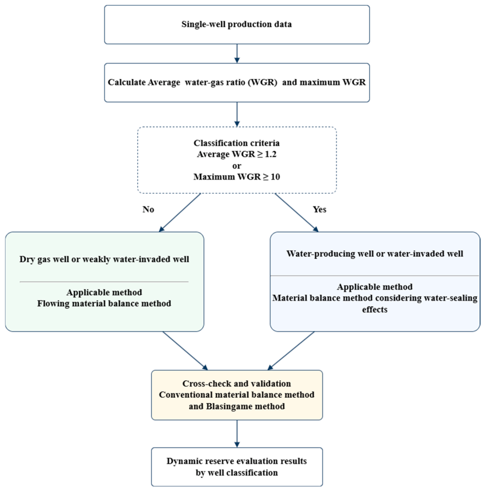
Water invasion affects the pressure and production responses of individual wells differently. Therefore, the same reserve evaluation method was not applied to every well. The average and maximum water–gas ratios (WGRs) were used to classify the wells. The WGR was expressed as the volume of produced water per 10⁴ m³ of produced gas, with a unit of m³/(10⁴ m³). The average WGR reflects the sustained level of water production over the production history, whereas the maximum WGR captures short-term increases associated with water breakthrough or intermittent water production.

Wells with an average WGR below 1.2 m³/(10⁴ m³) and a maximum WGR below 10 m³/(10⁴ m³) were classified as weakly water-affected gas wells. The FMB method was applied to these wells because water production had a limited influence on their pressure and production responses. Wells with an average WGR of 1.2 m³/(10⁴ m³) or higher, or a maximum WGR of 10 m³/(10⁴ m³) or higher, were classified as water-producing gas wells. Their dynamic reserves were evaluated using the material balance method accounting for the water-sealed gas effect. The conventional material balance method and Blasingame type curve analysis were used to cross-check the classified estimates. The thresholds of 1.2 and 10 m³/(10⁴ m³) were determined from the statistical distributions of the average and maximum WGRs, respectively, for all producing wells in the II-2 layer group.

As shown in Figure 1, the evaluation procedure consisted of compiling individual well production data, calculating the average and maximum WGRs, classifying the wells, and selecting the corresponding reserve evaluation method. The resulting well-level estimates were then aggregated to obtain the integrated dynamic reserves of the II-2 layer group and compared with the conventional material balance and Blasingame estimates.

2.3. Numerical Simulation and Identification of Water-Sealed Gas Potential

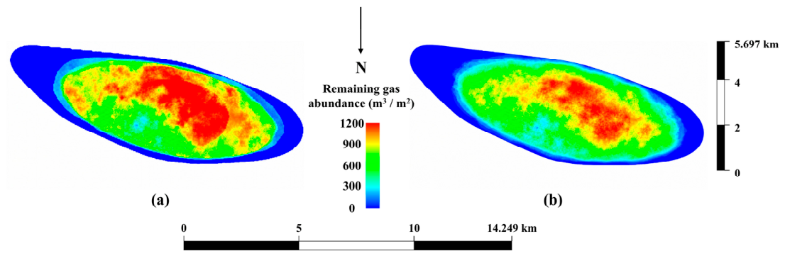
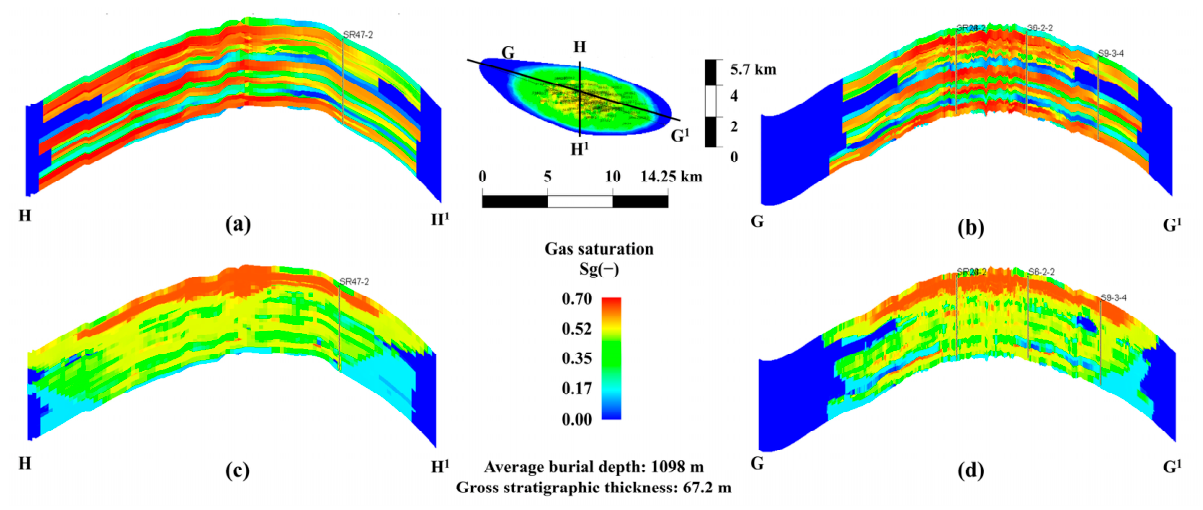
The classified well-level evaluation provides dynamic reserve estimates under different water production conditions. These estimates, however, do not reveal where the remaining gas is concentrated or how water invasion has altered its spatial distribution. A numerical model was therefore used to reconstruct gas–water redistribution and identify remaining gas enrichment at the areal, vertical, and sand-body scales.

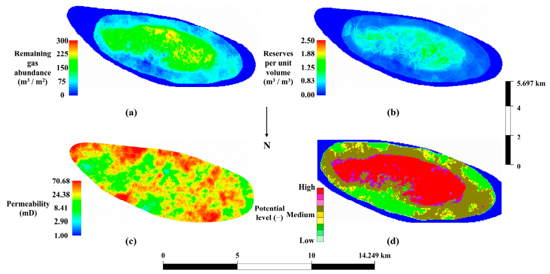
A three-dimensional gas–water model was constructed in Petrel (version 2021.1, Schlumberger) and simulated using ECLIPSE 100 (version 2021.1, Schlumberger). The model contains 285 × 114 × 39 corner-point grid cells, corresponding to 1,267,110 cells before inactive cells were excluded, and covers approximately 14.249 km × 5.697 km. The horizontal grid spacing is mainly 50 m, and the reservoir is divided vertically into 39 nonuniform layers. Porosity, permeability, initial water saturation, and other reservoir properties were transferred from the Petrel geological model and assigned cell by cell. Initial pressure was defined using a pressure–depth relationship, while edge water support was represented by a Fetkovich aquifer connected to the peripheral cells. The model used dry gas–water PVT data and one set of gas–water relative permeability curves, with a critical gas saturation of 0.156 and a connate water saturation of 0.359.

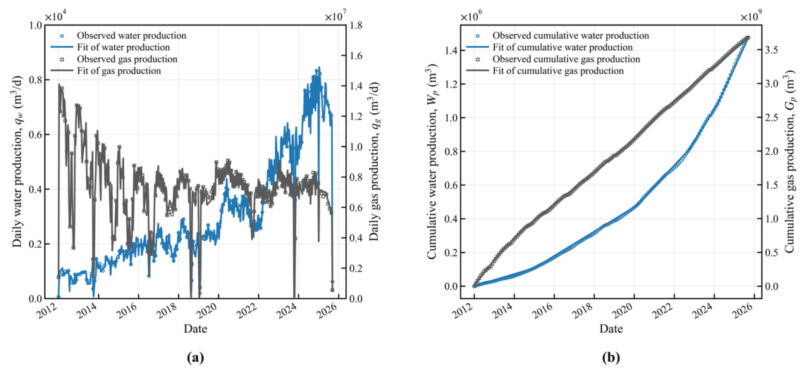
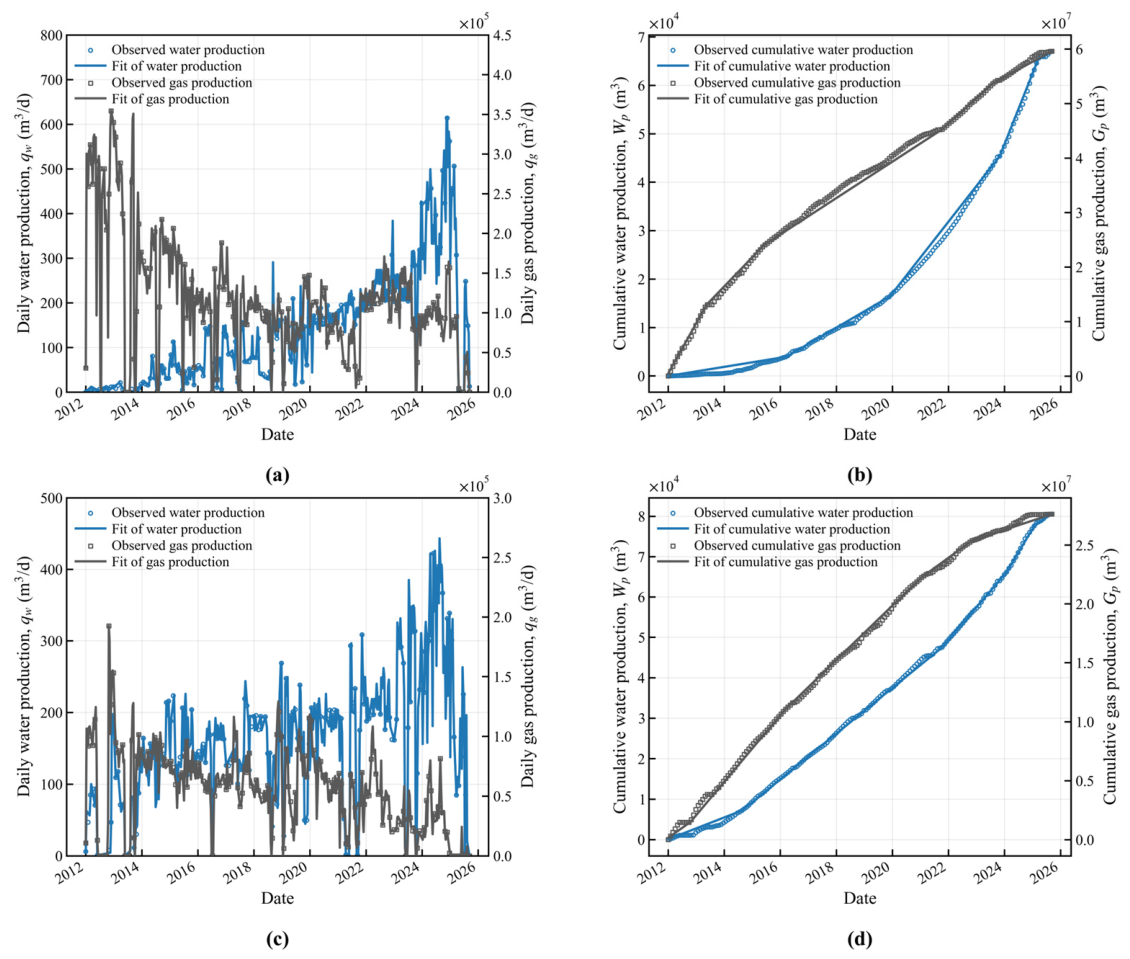
History matching was conducted against daily and cumulative gas and water production. The aquifer influx coefficient was adjusted to reproduce the overall water production response, while local permeability or transmissibility multipliers were modified to improve water breakthrough timing and individual well production behavior. The geological framework, initial conditions, and PVT properties were kept unchanged. For cumulative gas or water production, the relative error at the end of the history-matching period was calculated as:

$$E_k={\displaystyle \frac{\left|Q_{k,sim}-Q_{k,obs}\right|}{Q_{k,obs}}}\times 100\%,$$

(7)

where $Q_{k,sim}$ and $Q_{k,obs}$ are the simulated and observed cumulative production, respectively, and $k=g$ and $k=w$ denote gas and water. The matching score for each variable was defined as:

$$M_k=100\%-E_k.$$

(8)

The overall matching score was calculated as the arithmetic mean of the cumulative gas and cumulative water matching scores:

$$M_{overall}={\displaystyle \frac{M_g+M_w}{2}}.$$

(9)

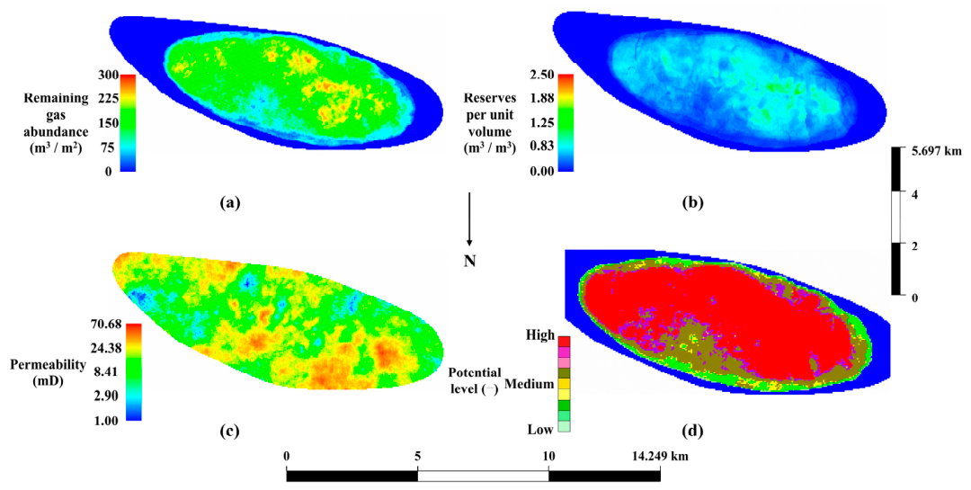
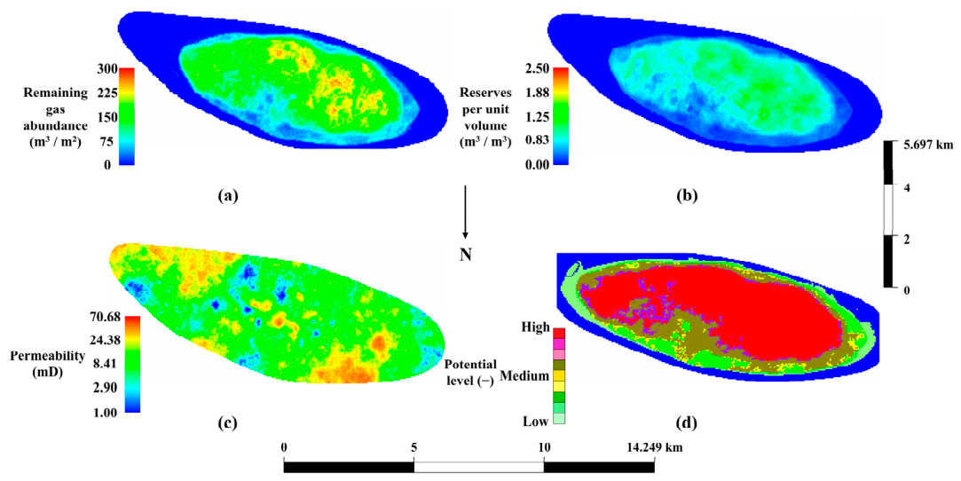
The gas and water production errors were also reported separately to avoid relying only on a single aggregate value. After history matching, remaining gas saturation, remaining gas-in-place abundance, reserves per unit volume, and permeability were extracted to identify water invasion pathways and remaining gas enrichment zones. The simulation results were then combined with the reserve estimates to evaluate water-sealed gas potential. For clarity, the mathematical symbols used in Equations (1)–(9) are summarized in

Table 1. Nomenclature of mathematical symbols used in Equations (1)–(9).

Symbol	Definition	Unit	Symbol	Definition	Unit
$p_i$, $p$, $p_c$	Initial, current, and tubing pressures, respectively	MPa	$Z_i$, $Z$, $Z_c$	Gas deviation factors corresponding to $p_i,p,$ and $p_c$, respectively	-
$G_p$	Cumulative gas production	108 m3	$G$	Gas reserve estimated by the corresponding method	108 m3
$W_e$, $W_p$	Cumulative water influx and water production, respectively	108 m3	$B_w$, $B_{gi}$	Water and initial gas formation volume factors, respectively	m3/m3
$\omega$	Water influx coefficient	-	$A$, $B$	Reservoir heterogeneity coefficient and water invasion constant, respectively	-
$R$	Gas recovery degree $G_p/G$	-	$a$, $b$	Intercept and slope of the FMB linear relationship	MPa; MPa/(108 m3)
$r_{eD}$, $r_{cD}$	Dimensionless external and matched drainage radii, respectively	-	$t_{caD}$, $t_{caDd}$	Dimensionless material balance times	-
$q_{Dd}$	Dimensionless decline rate	-	$t_{ca}$	Material balance time	d
$L^{-1}[{\overline{P}}_D]$	Inverse Laplace transform of average dimensionless pressure	-	$m_a$, $b_{pss}$	Slope and intercept obtained from type curve matching	-
$Q_{k,\mathrm{sim}}$, $Q_{k,\mathrm{obs}}$	Simulated and observed cumulative production	m3	$E_k$	Relative error of cumulative production	%
$M_k$, $M_{\mathrm{overall}}$	Individual and overall history-matching scores	%	$k$	Production variable index (g: gas; w: water)	-

.

Water invasion affects gas mobility differently across the reservoir. Therefore, water invasion types were classified before evaluating the distribution and mobility of remaining gas. The classification considered both dynamic and spatial responses to water invasion. WGR and pressure change reflect the production response to water entry, whereas the gas–water distribution reflects the spatial pattern of water advance and gas retention. The WGR range observed during the diagnostic water invasion stage, together with pressure decline and the simulated areal and vertical gas–water distributions, was used to characterize the water invasion pattern. Four categories were defined: channel invasion, uniform invasion, localized trapping, and non-invaded conditions. Because some WGR ranges overlap, WGR was not used as a single threshold. For the final classification, each producing well and its associated control area were assigned to a single dominant water invasion type by jointly considering the WGR response, pressure decline, and simulated areal and vertical gas–water distributions. The diagnostic criteria are summarized in

Table 2. Diagnostic criteria for water invasion types.

Water Invasion Type	Production Response	Stage WGR (m3/104 m3)	Pressure Decline (MPa)	Spatial Gas–Water Response
Channel invasion	Rapid WGR increase and relatively rapid pressure decline	10–30	>0.1	Preferential water advance along high-permeability or well-connected pathways, producing a spatially concentrated water invasion pattern
Uniform invasion	Gradual WGR increase at a relatively low level and slow pressure decline	5–10	0.05–0.1	Broad water advance without a distinct preferential pathway, with a relatively continuous gas–water transition
Localized trapping	Limited water-sealed volume with localized gas retention	10–20	>0.1	Localized water invasion associated with isolated or poorly connected remaining gas zones
Non invaded	No or very low liquid production	<2	<0.05	No evident water invasion pattern within the evaluated well-control area

.

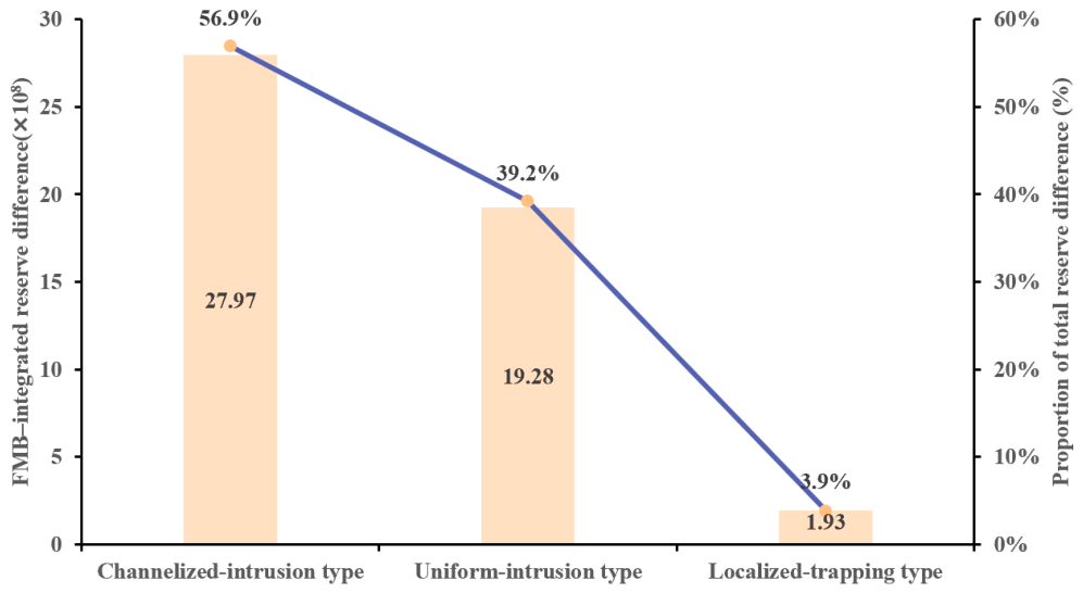
After each production well was assigned to one final water invasion type, the reserve difference was calculated at the well level. For well $i$, the difference was defined as $\Delta G_i=G_{FMB,i}-G_{\mathrm{int},i}$, where $G_{FMB,i}$ is the FMB estimate and $G_{\mathrm{int},i}$ is the reserve estimate adopted in the integrated evaluation. The reserve difference associated with each water invasion type was obtained by summing $\Delta G_i$ for all wells assigned to that type. Each well was assigned to only one final type. Therefore, the classified reserve differences were non-overlapping, and their sum was equal to the total difference between the FMB and integrated reserve estimates.

3. Results

3.1. Classified Dynamic Reserve Evaluation

Daily production data from the 113 wells were analyzed to describe the development history of the II-2 layer group. The water–gas ratio was calculated by dividing daily water production by daily gas production. Figure 2 shows an overall decline in gas production and a gradual increase in water production and the water–gas ratio, indicating that the influence of water invasion became stronger during development.

However, the layer group trend does not fully reflect the different responses of individual wells. Wells R15-2, R39-3, R40-3, R104-2, and R171-2 were selected because they have relatively complete records and represent different reservoir locations and production responses. Gas production rate and tubing pressure were normalized by dividing each current value by its initial value. As shown in Figure 3, water breakthrough occurred at different times among the wells and was generally associated with lower tubing pressure at later breakthrough stages. Gas production and tubing pressure also exhibited distinct temporal trends among the wells. The WGR of R40-3 increased relatively early, whereas those of R15-2 and R39-3 increased mainly during the later production period. In contrast, R104-2 and R171-2 maintained relatively low WGRs. These contrasting production responses indicate different degrees and timing of water invasion and provide the basis for subsequent well classification and reserve evaluation.

The conventional material balance method, the FMB method, Blasingame type curve analysis, and the material balance method accounting for the water-sealed gas effect were applied to evaluate the dynamic reserves of the II-2 layer group. Because the wells in this layer group exhibit different degrees of water production, the resulting dynamic reserve estimates are influenced by the applicability conditions of the individual methods. The evaluation results were therefore compared by considering both the water production characteristics of individual wells and the estimates obtained using the different methods.

As shown in

Table 3. Individual well classification and dynamic reserve evaluation results for the II-2 layer group.

Well	Average WGR	Maximum WGR	Well Category	FMB Method (108 m3)	Blasingame Type Curve Analysis (108 m3)	Material Balance Method Accounting for the Water-Sealed Gas Effect (108 m3)
R15-2	19.70	1323.68	Water-producing gas well	1.48	1.14	1.07
R39-3	13.17	157.58	Water-producing gas well	0.97	1.99	0.97
R40-3	8.99	258.13	Water-producing gas well	0.83	0.46	0.8
R104-2	0.19	0.83	Weakly water-affected gas well	2.31	0.66	0.71
R171-2	0.41	2.74	Weakly water-affected gas well	0.66	0.41	0.22

and Figure 4, both the water production characteristics and dynamic reserve estimates vary among the individual wells. Wells R15-2, R39-3, and R40-3 have average WGRs of 19.70, 13.17, and 8.99, respectively, and maximum WGRs of 1323.68, 157.58, and 258.13, respectively; these wells were therefore classified as water-producing gas wells. Wells R104-2 and R171-2 have average WGRs of 0.19 and 0.41, respectively, and maximum WGRs of 0.83 and 2.74, respectively; they were classified as weakly water-affected gas wells. The corresponding individual well reserve estimates also differ among the methods. For well R15-2, the FMB method, Blasingame type curve analysis, and the material balance method accounting for the water-sealed gas effect yielded reserve estimates of 1.48, 1.14, and 1.07 × 10⁸ m³, respectively. For well R171-2, the corresponding estimates were 0.66, 0.41, and 0.22 × 10⁸ m³, respectively. These results demonstrate that the dynamic reserve estimates for individual wells in the II-2 layer group vary among the different methods. Applying a single method to all wells may therefore fail to adequately represent wells with different water production responses.

Table 4. Dynamic reserve estimates for the II-2 layer group obtained using different methods.

Layer Group	Conventional Material Balance Method (108 m3)	FMB Method (108 m3)	Blasingame Type Curve Analysis (108 m3)	Material Balance Method Accounting for the Water-Sealed Gas Effect (108 m3)
II-2	77.93	119.90	87.41	64.04

summarizes the layer–group–scale evaluation results. The dynamic reserves calculated using the conventional material balance method, the FMB method, Blasingame type curve analysis, and the material balance method accounting for the water-sealed gas effect are 77.93, 119.90, 87.41, and 64.04 × 10⁸ m³, respectively. The FMB method yields the highest estimate, whereas the material balance method accounting for the water-sealed gas effect yields the lowest. The difference between the two estimates is 55.86 × 10⁸ m³, indicating that the dynamic reserve estimates for the II-2 layer group vary substantially among the methods.

Taken together, the individual well and layer–group–scale results indicate that the dynamic reserve evaluation of the II-2 layer group is sensitive to the method selected. To avoid biases associated with using a single evaluation method, the results should be assessed comprehensively by considering well classification, method applicability, and the estimates obtained using the different methods.

3.2. Integrated Dynamic Reserve Evaluation and Classification of the Reserve Difference

As summarized in

Table 5. Reserve balance and comparison of reserve estimates for the II-2 layer group.

Layer Group	FMB Method (108 m3)	Integrated Dynamic Reserves (108 m3)	Cumulative Gas Production (108 m3)	Remaining Recoverable Reserves (108 m3)	FMB-Integrated Reserve Difference (108 m3)
II-2	119.90	70.72	36.81	33.91	49.18

, the integrated dynamic reserves of the II-2 layer group are 70.72 × 10⁸ m³. This estimate was obtained by first classifying the producing wells according to their water production characteristics. The FMB method was applied to weakly water-affected gas wells, whereas the material balance method accounting for the water-sealed gas effect was applied to water-producing gas wells. The individual well estimates were then aggregated to obtain the integrated result. This value differs from the estimates obtained using the conventional material balance method, the FMB method, Blasingame type curve analysis, or the material balance method accounting for the water-sealed gas effect alone. In those evaluations, the same method was applied to all wells, whereas the integrated evaluation selected the method that better matched the water invasion response of each well.

The remaining recoverable reserves were then determined from the integrated dynamic reserves after accounting for cumulative gas production. The reserve balance is expressed as $G_{rem}=G_{dyn}-G_p$, where $G_{rem}$ is the remaining recoverable reserve, $G_{dyn}$ is the integrated dynamic reserve, and $G_p$ is the cumulative gas production up to the evaluation date. As of 31 August 2025, the cumulative gas production of the II-2 layer group was 36.81 × 10⁸ m³. The corresponding remaining recoverable reserves were 33.91 × 10⁸ m³ based on the field reserve evaluation.

The FMB estimate of 119.90 × 10⁸ m³ was used as a reference because the method does not explicitly account for the reduction in gas mobility associated with water production. The difference between the FMB estimate and the integrated dynamic reserve estimate is 49.18 × 10⁸ m³. Because the two estimates are based on different assumptions and method applicability, this difference cannot be attributed solely to water invasion. It is therefore used as an indirect indicator of restricted gas mobilization under the current water invasion conditions.

The FMB-integrated reserve difference was further classified according to the identified water invasion patterns into channel invasion, uniform invasion, and localized trapping types. As shown in

Table 6. Classification of the FMB-integrated reserve difference by water invasion type.

Water Invasion Type	Reserve Difference (108 m3)	Proportion (%)	Principal Controlling Factor	Potential Recovery Strategy
Channel invasion type	27.97	56.9	Water invasion along preferential flow channels and isolation of remaining gas	Selective water shutoff after identifying preferential water invasion pathways
Uniform invasion type	19.28	39.2	Continuous water advance and reduced gas-phase mobility	Water block removal and flow resistance reduction
Localized trapping type	1.93	3.9	Poor local connectivity and retention of remaining gas	Improvement of local reservoir connectivity
Total	49.18	100.0	-	-

and Figure 5, the corresponding reserve differences associated with channel invasion, uniform invasion, and localized trapping are 27.97, 19.28, and 1.93 × 10⁸ m³, accounting for 56.9%, 39.2%, and 3.9%, respectively. Together, the reserve differences associated with channel invasion and uniform invasion account for 96.1% of the total reserve difference, indicating that the reserve difference is concentrated mainly in wells characterized by these two water invasion types.

3.3. Spatial Identification Through Numerical Simulation

Following the classified dynamic reserve evaluation, a history-matched numerical simulation model was used to further characterize the spatial distribution of remaining gas in the II-2 layer group. Figure 6 compares the observed and simulated production performance of the II-2 layer group. The simulated cumulative gas and water production closely follow the observed trends, with estimated relative errors of 3.47% and 6.21%, respectively, at the end of the history-matching period. The resulting overall matching score is approximately 95.16%. Figure 7 further shows that the model generally reproduces the production responses of representative wells R15-2 and R30-2. Although some differences remain in the daily production rates because of short-term changes in well operating conditions, the cumulative production curves show good agreement. The model therefore captures the main gas depletion and water invasion trends and provides a reasonable basis for analyzing the spatial distribution of remaining gas.

As shown in Figure 8, the average gas saturation of the II-2 layer group exhibits pronounced areal variations at the end of the simulation. Gas saturation is relatively low along the reservoir margins, indicating a substantial influence of edge water invasion. In contrast, localized areas in the central and eastern parts of the layer group retain relatively high gas saturation and therefore represent zones of remaining gas enrichment. As shown in Figure 9, the extent of the high-value remaining gas-in-place abundance zones decreased after development compared with that at the beginning of the simulation. Areas with relatively high remaining gas-in-place abundance are mainly preserved in the central and eastern parts of the layer group and locally in the northern part, indicating that the distribution of remaining gas is jointly controlled by the extent of water invasion and the initial gas-in-place abundance.

Figure 10 presents changes in gas saturation along north–south and east–west cross-sections through the II-2 layer group. At the beginning of the simulation, gas saturation was generally high in all intervals. At the end of the simulation, gas saturation had decreased markedly along the margins of the II-2 layer group and in some lower intervals, whereas certain upper sand bodies and structurally higher areas retained appreciable gas saturation. These results indicate that water invasion affects the different intervals to varying degrees and that the vertical distribution of remaining gas is heterogeneous.

At the individual interval scale, Figure 11 and Figure 12 show that intervals 2-5-11 and 2-5-12 contain localized areas with relatively high remaining gas-in-place abundance and reserves per unit volume, indicating appreciable potential for further remaining gas recovery. The permeability distributions within both intervals are heterogeneous, demonstrating strong internal reservoir heterogeneity. Subsequent recovery target selection should therefore consider both the locations of remaining gas enrichment and the distribution of high-permeability channels. Figure 13 shows that interval 2-6-13 contains locally high-permeability areas but has relatively low remaining gas-in-place abundance and reserves per unit volume. This interval therefore exhibits relatively weak remaining gas enrichment and is more suitable for identifying water invasion pathways.

3.4. Water Invasion Types and Potential Development Intervals

Potential target intervals were identified by integrating the water invasion classification with the simulated distributions of remaining gas and permeability. As summarized in

Table 7. Remaining gas enrichment zones, water invasion types, and potential recovery strategies for the II-2 layer group.

Potential Target	Identification Criteria	Dominant Water Invasion Type	Principal Problem	Potential Recovery Strategy
2-5-11	Locally high remaining gas-in-place abundance and reserves per unit volume; heterogeneous permeability distribution	Channel-invasion type	Isolation of remaining gas by water channeling	Selective water shutoff after identifying water-channeling pathways
2-5-12	Localized concentration of remaining reserves; heterogeneous permeability distribution	Predominantly channel-invasion type	Water invasion-induced permeability impairment	Water control combined with water block removal or flow resistance reduction

, intervals 2-5-11 and 2-5-12 contain localized zones with relatively high remaining gas-in-place abundance and reserves per unit volume, together with heterogeneous permeability distributions. Interval 2-5-11 was classified mainly as a channel invasion type, while interval 2-5-12 was classified as predominantly channel-invasion type. These two intervals were therefore selected as potential targets for further evaluation. By comparison, interval 2-6-13 has lower remaining gas-in-place abundance and reserves per unit volume and was not selected as a principal target interval.

4. Discussion

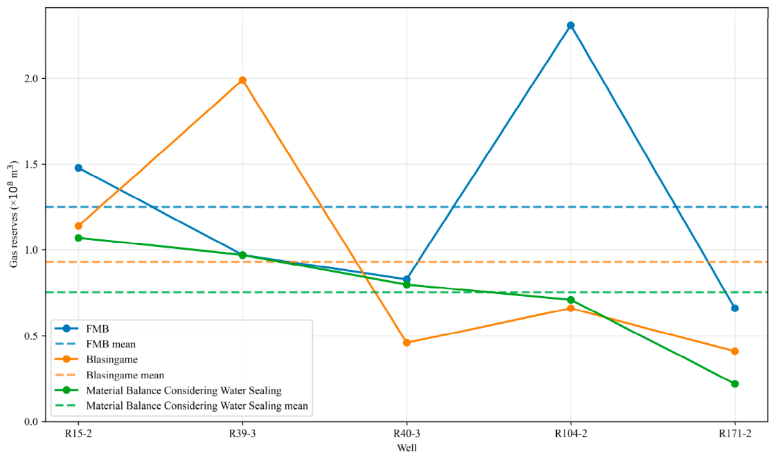
The marked differences among the reserve estimates indicate that water production complicates the relationship between pressure response and gas producibility. Gas may remain in pressure communication with producing wells while its effective mobility is reduced by water invasion. Previous studies have incorporated reservoir heterogeneity and water invasion effects into the evaluation of water-sealed gas behavior [24,25]. In the present workflow, the FMB-integrated reserve difference is therefore used as a comparative indicator of reduced reserve producibility under water invasion, while its magnitude may also reflect differences in method assumptions, pressure representation, and local reservoir connectivity. The contribution of the present workflow lies in applying reserve evaluation methods according to individual well water production responses and linking the resulting estimates with water invasion classification and three-dimensional remaining gas characterization. This integration provides a field-scale basis for interpreting reserve differences by combining multiple diagnostic dimensions, thereby reducing the bias associated with reliance on a single evaluation method.

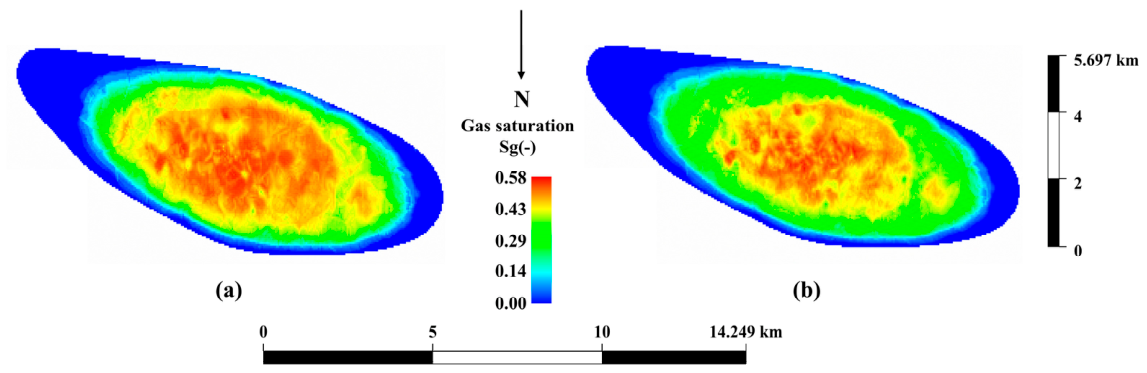
The dominance of channel and uniform invasion patterns is consistent with the strong heterogeneity of the II-2 layer group. Preferential water advance through high-permeability and well-connected zones can produce rapid water breakthrough and locally isolate remaining gas, whereas broader water advance reduces gas mobility over a larger reservoir area [1,2,9,29]. Unlike material balance classifications based primarily on recharge and sealing characteristics, the categories used here are defined from combined production and spatial responses and are intended to describe the dominant water invasion behavior around individual wells. The numerical simulation supports this interpretation. Gas saturation decreases markedly near the reservoir margins, while relatively high remaining gas saturation is preserved mainly in structural highs and in parts of the central and eastern reservoir. Physical simulation has shown that reservoir heterogeneity and preferential flow pathways strongly influence water invasion and residual gas distribution [29]. Numerical studies further demonstrate that reservoir connectivity and preferential pathways control the spatial evolution of water invasion [30,32]. These results suggest that the spatial distribution of remaining gas is controlled by both water invasion pathways and local reservoir connectivity, rather than by the degree of water production alone.

These differences in water invasion behavior also have implications for subsequent development. Where channelized invasion dominates, preferential water pathways may need to be controlled before the remaining gas can be effectively mobilized [33]. In areas affected by broader water invasion, reducing water blocking and restoring gas-phase flow capacity may be more important [34]. The relatively high remaining gas abundance identified in intervals 2-5-11 and 2-5-12 therefore indicates development potential, but these intervals should be regarded as candidate targets rather than confirmed targets. The workflow is most applicable to mature water-invaded gas reservoirs with sufficiently long production histories and a calibrated gas–water model, whereas the classification thresholds require reservoir-specific calibration before application to other fields. WGR and pressure responses can also be affected by operating conditions, completion intervals, and local connectivity, while the simulated remaining gas distribution depends on the permeability model, aquifer representation, relative permeability curves, and history matching. Further well-specific simulation and field verification are therefore required before development measures are implemented.

5. Conclusions

This study combined classified well-level reserve estimates with numerical simulation to evaluate dynamic reserves and remaining gas potential in the II-2 layer group of the Sebei-2 Gas Field. The main conclusions are as follows:

(1) Reserve estimates vary markedly among methods, showing that a single method cannot adequately represent wells with different water production responses. The classified approach gives dynamic reserves of 70.72 × 10⁸ m³, of which 33.91 × 10⁸ m³ remain recoverable. The FMB estimate exceeds the integrated estimate by 49.18 × 10⁸ m³. This method-dependent difference is an indirect indicator of restricted gas mobilization under the current water invasion conditions.

(2) The reserve differences associated with channel invasion and uniform invasion account for 56.9% and 39.2% of the total FMB-integrated reserve difference, respectively, together representing 96.1% of the total. The model places the main remaining gas accumulations in structural highs and in the central and eastern parts of the reservoir, with additional local enrichment in the north.

(3) Intervals 2-5-11 and 2-5-12 are candidate intervals for further development evaluation because they contain relatively high remaining gas-in-place abundance and reserves per unit volume. Selective water shutoff may be considered where channelized invasion dominates, whereas water block removal or flow resistance reduction may help where water has reduced gas mobility. These measures have not been tested through scenario simulations and therefore require well-specific modeling and field verification before implementation.