Research Progress of Multi-Source Sensing Technology and Intelligent Modeling Methods in Vegetation Monitoring

Abstract

This review comprehensively summarizes the recent research progress of multi-source sensing technologies and intelligent modeling methods in vegetation monitoring. It elucidates the physical mechanisms and complementary natures of core active and passive technologies, including optical hyperspectral remote sensing, LiDAR structural detection, and microwave/millimeter-wave radar. Furthermore, it systematically analyzes advanced data processing methods, covering physics-based radiative transfer models, data-driven machine learning, Physics-Data Dual-Driven Modeling transfer learning, and multi-source data fusion strategies. The paper highlights successful applications across diverse typical scenarios, such as crop precision nitrogen diagnosis, forest biomass estimation, crop lodging risk prediction, and vegetation stress assessment. Finally, it discusses critical challenges like data heterogeneity and model generalization, while presenting a future outlook focused on building collaborative “space-air-ground” integrated monitoring networks and advanced AI fusion methods.

1. Introduction

The compounding effects of continuous global population growth and climate change pose severe challenges to agricultural productivity and forest ecosystem service functions [1,2]. As the largest carbon pool in terrestrial ecosystems, the carbon sequestration capacity of forests is under continuous threat from forest degradation, wildfires, pests, and diseases [3]. In this context, the precise monitoring of crop growth and forest structural dynamics has become a critical pillar for ensuring food security and addressing climate change.

Core parameters of vegetation monitoring encompass crop physiological and biochemical indicators as well as forest structural characteristics [4]. At the crop level, nitrogen status directly regulates yield and quality, making its precise monitoring a prerequisite for achieving on-demand fertilization and improving nitrogen use efficiency [5,6]; leaf water content and canopy moisture status influence photosynthetic efficiency and drought resistance; biomass and leaf area index (LAI) serve as critical inputs for carbon and water cycle simulations [7,8].

In forest ecosystems, tree height, LAI, and aboveground biomass are not only the basis for carbon stock estimation but also reflect forest health and succession dynamics [9]. The significant impact of lianas on the canopy structure and chemical composition of tropical forests further highlights the ecological value of fine-scale canopy monitoring [10]. Traditional monitoring relies on destructive field sampling, which, despite yielding accurate results, is time-consuming, costly, lacks timeliness, and has limited spatial coverage. This is particularly challenging in forest stands with diverse tree species and complex structures, and it fails to capture spatial heterogeneity at the field or landscape scale.

The rapid development of remote sensing and sensing technologies has provided new means for vegetation monitoring [11,12]. Satellites, manned aircraft, unmanned aerial vehicles (UAVs), and near-ground sensors form a multi-platform stereoscopic monitoring system. Satellite remote sensing offers global coverage, and multispectral and hyperspectral data have been widely used for vegetation index inversion and LAI product generation; however, constrained by revisit cycles, cloud interference, and spatial resolution, its capacity for fine-scale monitoring remains insufficient [13,14]. UAV platforms bridge the scale gap between satellite and ground observations, and owing to their flexibility, high spatiotemporal resolution, and low-cost advantages, they have been extensively applied in vegetation monitoring in recent years [15,16]. At the sensor level, the complementarity between active and passive technologies is becoming increasingly evident. Optical sensors retrieve biochemical parameters such as chlorophyll, carotenoids, and nitrogen by measuring canopy reflectance spectra, with hyperspectral sensing performing exceptionally well in constituent inversion due to its narrow-band advantages; however, passive optics are susceptible to illumination and cloud coverage, and signal saturation issues are prominent under high LAI conditions [17]. LiDAR, as an active remote sensing technology, accurately delineates tree height, vertical canopy profiles, and LAI by emitting laser pulses, independent of light conditions [18,19,20]. Zeng et al. (2026) introduced the canopy gap size distribution theory and proposed a correction method targeting the LiDAR beam footprint effect, significantly improving the accuracy of LAI estimation [21]. However, substantial variations exist in the beam divergence angle, pulse energy, and penetration capacity among different LiDAR systems, necessitating the development of corresponding correction methods. Microwave Synthetic Aperture Radar (SAR) and Frequency-Modulated Continuous-Wave (FMCW) radar possess all-time and all-weather capabilities, enabling effective detection even under smoke and cloud conditions [22,23,24]. Horst et al. (2019) and Gao et al. (2019) systematically analyzed the impacts of frequency uncertainty and translational position errors on microwave SAR imaging and proposed compensation methods, laying the foundation for microwave radar applications in vegetation monitoring [25,26]. Janpangngern et al. (2025) achieved small UAV detection using a high-resolution FMCW radar based on software-defined radio, demonstrating the capability to detect weak targets in complex environments [27]. Schenkel et al. (2024) utilized millimeter-wave radar to achieve smoke detection and combustion analysis, proving that the sensitivity of radar signals to changes in the dielectric constant of media can be utilized for dynamic fire monitoring [28].

Regarding data processing, traditional empirical models suffer from weak generalization capabilities, while physical models face ill-posed inversion problems, each presenting its own limitations. Machine learning and deep learning methods, by virtue of their powerful non-linear fitting capabilities, have demonstrated prominent advantages in vegetation parameter inversion. Lu et al. (2022) utilized random forest regression to fuse multi-source data, significantly improving the prediction accuracy of the rice nitrogen nutrition index [29]. Yang et al. (2026) coupled the N-PROSAIL radiative transfer model with deep transfer learning to achieve high-precision estimation of canopy nitrogen density in winter wheat, effectively mitigating the overfitting issue caused by small sample sizes [30]. Multi-source data fusion significantly enhances the accuracy of nitrogen diagnosis and fertilization recommendations by integrating sensor data, environmental factors, and agronomic management information [31].

This paper systematically reviews the principles, methods, applications, and challenges of multi-source sensing technologies in vegetation monitoring. Although agricultural crops and forest ecosystems share common sensing principles and data processing frameworks, they differ substantially in canopy structure, growth characteristics, spatial scale, and monitoring objectives. Therefore, this review discusses the application of multi-source sensing technologies in different vegetation scenarios. Specifically, crop monitoring mainly focuses on physiological and biochemical parameters, such as nitrogen status, water content, and growth conditions, whereas forest monitoring emphasizes structural parameters, biomass estimation, and ecosystem-scale assessment. The objective of this review is to summarize the common technical foundations while highlighting the specific requirements and adaptations for different vegetation types.

2. Fundamentals of Stereo Vision and Adaptation to Agricultural Environments

However, the retrieved vegetation parameters and practical applications vary considerably between agricultural crops and forest ecosystems. Crop monitoring generally focuses on dynamic physiological and biochemical characteristics, such as nitrogen status, water content, and growth conditions, due to relatively uniform canopy structures and short growth cycles. In contrast, forest monitoring emphasizes three-dimensional structural characteristics, biomass estimation, and ecosystem-scale assessment because of complex canopy architectures and long-term ecological processes. Therefore, although similar sensing technologies can be employed, parameter selection, data acquisition strategies, and modeling approaches should be adapted according to vegetation type [32,33,34].

2.1. Construction and Computational Pipeline of Binocular Stereo Vision Systems

The core of passive optical remote sensing lies in detecting the spectral characteristics of solar radiation reflected by the vegetation canopy. Pigments, water, and cellular structures within vegetation leaves exhibit selective absorption and reflection characteristics across specific electromagnetic radiation bands, thereby forming spectral signals that can be used to retrieve vegetation physiological and biochemical parameters [35,36].

In the visible region (400–700 nm), chlorophyll a and chlorophyll b exhibit strong absorption peaks in the blue (approx. 430 nm, 450 nm) and red (approx. 660 nm, 670 nm) bands, while the reflectance is relatively higher in the green band (approx. 550 nm), which is the direct reason vegetation appears green. At the boundary between red and near-infrared light (approx. 700–1300 nm), vegetation reflectance rises sharply, forming the so-called “red-edge effect,” whose position and slope are highly sensitive to chlorophyll content, nitrogen status, and stress responses [37]. In the shortwave infrared region (1300–2500 nm), water absorption bands at approximately 1450 nm and 1940 nm dominate the spectral features, which can be utilized to estimate vegetation water content [38]. Hyperspectral remote sensing, by virtue of its capacity to detect dozens to hundreds of contiguous narrow bands, can capture these fine spectral signatures, thereby achieving quantitative inversion of vegetation biochemical components.

Ferreira et al. (2025) utilized UAV-borne hyperspectral data (400–1000 nm) to study the effects of liana removal on the canopy chemical composition of tropical seasonal forests [39]. The study calculated 87 vegetation indices and found that during the dry season, pigment-sensitive indices exhibited a moderate-to-large negative response to liana removal. Among them, the Pigment Absorption Ratio Shortwave (PARS) index showed the strongest response (Cohen’s d = −0.595, coefficient of variation 13.7%), and the effect sizes of the Green Modified Index (GMI2) and Simple Ratio indices (SR1–SR3) also reached −0.548 to −0.566. These results indicate that canopy greenness significantly decreased following liana removal, because evergreen lianas rely on their deep root systems to maintain leaves during the dry season, whereas trees shed their leaves during this period, making lianas the primary contributor to canopy greenness. In contrast, the effect sizes of wet season indices (such as Double Difference index DD, Optimized Soil-Adjusted Vegetation Index OSAVI2, and Modified Soil-Adjusted Vegetation Index MSAVI) were negligible (Cohen’s d < 0.2), indicating that under resource-abundant conditions, both trees and lianas fully flush their leaves, obscuring competitive differences [39]. Figure 1 shows the cross-section view of raw point clouds obtained by backpack LiDAR, UAV LiDAR, as well as their fused point cloud, which reveals their respective advantages and deficiencies in vegetation point-cloud capturing.

In the field of crop monitoring, active canopy sensors (such as Green Seeker and Crop Circle ACS-430) represent an important extension of optical remote sensing technology [40,41]. Unlike passive sensors that depend on solar light sources, active sensors carry their own light sources and are unaffected by changes in ambient lighting, enabling them to acquire stable canopy reflectance data under diverse weather conditions. The Green Seeker sensor calculates the Normalized Difference Vegetation Index (NDVI) and Ratio Vegetation Index (RVI) using two bands: red (656 nm) and near-infrared (770 nm). In a two-year field trial on pak choi, NDVI and RVI exhibited correlation coefficients with aboveground biomass of 0.698–0.967 and 0.642–0.951, respectively, and with plant nitrogen uptake of 0.678–0.951 and 0.677–0.951, respectively. In independent modeling across four growth stages, RVI achieved the highest estimation accuracy for biomass during the seedling and rosette stages (R² reaching 0.80–0.94), whereas NDVI performed better during the heading and maturity stages (R² reaching 0.63–0.91). Incorporating the number of days in the growth period into multiple linear models improved the estimation accuracy of biomass by 19.0–35.6% for NDVI and 40.4–84.6% for RVI [42,43,44]. To visually distinguish the performance differences between active canopy sensors and traditional chlorophyll meters in crop nitrogen monitoring, the relevant statistical results of the two types of equipment are summarized in

Table 1. Correlation Comparison Table between Green Seeker Active Sensor and SPAD Chlorophyll Meter.

Sensor Index	The Correlation Coefficient with AGB (r)	The Correlation Coefficient with PNU (r)	Sources of Data
NDVI (GreenSeeker)	0.698–0.967	0.678–0.951	Ji et al. (2020)
RVI (GreenSeeker)	0.642–0.951	0.677–0.951	Ji et al. (2020)
SPAD (Chlorophyll Meter)	Not significant in the early stage; lower than the sensor value in later stages.	—	Ji et al. (2020)

.

The Crop Circle ACS-430 sensor further extends the band configuration by adding a red-edge band (730 nm) in addition to the red (670 nm) and near-infrared (780 nm) bands. The introduction of the red-edge band enables it to calculate indices that are more sensitive to chlorophyll and nitrogen, such as the Normalized Difference Red Edge index (NDRE) and the Canopy Chlorophyll Index (CIRE) [45]. Dong et al. (2023) utilized Crop Circle ACS-430 to collect canopy reflectance data during the maize V8 growth stage (late jointing stage) [46], and combined it with environmental and agronomic variables such as planting density, nitrogen application rate, growing degree days, and cumulative precipitation to establish a prediction model for maize stem lodging risk. The study found that among the 35 vegetation indices tested, three-band indices based on red-edge and near-infrared bands (such as MCARI2/REOSAVI, MTCARI, NDI) achieved the best prediction performance for lodging-related parameters, with R² ranging from 0.67 to 0.84. After incorporating multi-source data into multiple linear regression (MLR), the prediction R² for lodging risk indicators (stem failure moment and critical wind speed) improved from 0.34–0.67 in simple regression to 0.69–0.83, with a significant reduction in root mean square error [46]. To quantify the enhancement effect of multi-source variable fusion on lodging prediction accuracy, the prediction indicators of different regression schemes are organized in

Table 2. Prediction Accuracy Comparison Table of Multiple Regression Methods for Maize Lodging Risk.

Prediction Goal	Regression Method	R2	RMSE	Sources of Data
Natural Frequency	Simple Regression (Optimal Spectral Index)	0.75	—	Dong et al. (2023) [46]
Natural Frequency	MLR (Multi-source Data Fusion)	0.83	—	Dong et al. (2023) [46]
Plant Height	Simple Regression (Optimal Spectral Index)	0.82	—	Dong et al. (2023) [46]
Plant Height	MLR (Multi-source Data Fusion)	0.87	—	Dong et al. (2023) [46]
Stem Failure Moment	Simple Regression (Optimal Spectral Index)	0.67	3.73 Nm	Dong et al. (2023) [46]
Stem Failure Moment	MLR (Multi-source Data Fusion)	0.83	2.69 Nm	Dong et al. (2023) [46]
Critical Wind Speed (Direct)	Simple Regression (Optimal Spectral Index)	0.43	0.79 m/s	Dong et al. (2023) [46]
Critical Wind Speed (Direct)	MLR (Multi-source Data Fusion)	0.69	0.58 m/s	Dong et al. (2023) [46]

.

2.2. Active Structural Detection Based on LiDAR

LiDAR (Light Detection and Ranging) precisely calculates the distance between the sensor and the target by emitting laser pulses and measuring their return time after reflecting off the target (i.e., Time of Flight method) [47,48]. Unlike passive optical remote sensing, LiDAR does not rely on solar illumination, can operate day and night, and its laser pulses possess a certain degree of penetration capability, allowing them to pass through canopy gaps to obtain understory ground information, thereby achieving direct measurement of three-dimensional vegetation structure [49,50].

The core of LiDAR data processing lies in the generation and classification of point clouds. Original point clouds undergo denoising, filtering, and classification processing to distinguish ground points from non-ground points [51]. A Digital Elevation Model (DEM) is generated based on ground point interpolation, and a Digital Surface Model (DSM) is generated based on all points (primarily first returns); subtracting the former from the latter yields the Canopy Height Model (CHM). Each pixel value of the CHM represents the height of vegetation above the ground surface at that position, serving as the foundational data product for estimating tree height, crown width, gap fraction, and vertical canopy structure [52].

Regarding tree height estimation, Thinley et al. (2025) selected an urban arboretum in Queensland, Australia, containing 56 tree species with a stand age of approximately 10 years as the research subject [53]. They used UAV LiDAR data to generate a CHM and compared it with field-measured data from 287 trees. The study found that the Pearson correlation coefficient between the CHM and measured tree height reached 0.85, and the coefficient of determination R² of linear regression was 0.73 (Tree Height = 1.94 + 0.85 × CHM). For aboveground biomass estimation, the log-linear regression R² of the CHM was 0.43. Notably, the inclusion of Sentinel-2 satellite-derived vegetation indices (NDVI, EVI, LAI) into the model did not significantly improve the estimation accuracy of individual tree biomass, demonstrating that high-resolution LiDAR structural information carries more informative value than medium-resolution spectral information in a mixed-species urban forest [54,55,56].

In terms of leaf area index (LAI) inversion, Zeng et al. (2026) [21] conducted a systematic study on the impact of the LiDAR beam footprint effect on canopy gap fraction estimation. The study compared the LAI inversion accuracy of two LiDAR systems across 29 forest plots: Livox (large beam divergence angle, elliptical footprint of approximately 52 mm × 489 mm) and RIEGL VUX-1LR (small beam divergence angle, footprint of approximately 50 mm × 50 mm at a 100 m altitude) [21]. The study discovered that the Livox system, with its larger beam footprint, severely underestimated the canopy gap fraction (with a bias reaching −50.5%), leading to an overestimation of LAI by 42.3%. Zeng et al. proposed a correction method based on canopy gap size distribution theory, introducing a Normalized Penetration Quality Index (NPQI) and adaptive weight factors to compensate for missed small-scale gaps [21]. Post-correction, the gap fraction estimation R² of Livox improved from 0.63 to 0.73, and the RMSE dropped from 0.06 to 0.03; the RMSE of LAI estimation dropped drastically from 2.12 to 0.54. For the RIEGL system, the correction effect was minimal at a 200 m altitude (RMSE decreased from 0.37 to 0.35), but at a 300 m altitude, due to the increased beam footprint, the post-correction RMSE decreased from 0.74 to 0.37. The study also found that, along the vertical profile, the 10th percentile height of the Livox point cloud shifted upward to 12.25 m in dense forest plots, whereas the RIEGL system was still able to capture near-surface returns at heights of 3.5 m and 5.25 m at flight altitudes of 200 m and 300 m, respectively. These findings indicate that canopy penetration is strongly affected by sensor characteristics, including beam divergence, footprint size, and pulse energy, rather than by point cloud density alone. The influence of sensor configuration on the vertical representation of forest structure can also be observed in the representative cross-sections shown in Figure 2, which compare point clouds acquired over the same broadleaved forest site using five different UAV LiDAR systems.

Subedi and Zurqani (2026) further evaluated the effects of flight speed and image overlap on the quality of UAV LiDAR data [57]. The study found that LiDAR point cloud density increases with higher image overlap, with a flight speed of 10 mph combined with an 80:80 forward/side overlap yielding the highest point cloud density (437.8 pts/m²), which is more than three times that of the 50:50 overlap configurations. However, the canopy height percentiles (P25, P50, P75, P95) inverted by LiDAR showed no significant differences among various configurations, indicating that once point cloud density reaches a certain threshold, continuing to increase overlap yields limited improvement for canopy structural parameters. Regarding tree height estimation accuracy, UAV-LiDAR performed best under 10 mph and 80:80 overlap conditions (R² ≈ 0.89, RMSE < 1.5 m, bias < 0.5 m), and maintained high consistency across all flight configurations, showcasing the superior robustness of LiDAR compared to optical imagery. To clearly compare the tree height inversion accuracy between UAV photogrammetry and LiDAR under different flight parameters, the relevant experimental results are summarized in

Table 3. Tree Height Estimation Accuracy Comparison under Different Sensors (UAV Imagery SfM/UAV-LiDAR).

Sensor Type	Flight Speed (mph)	Overlap Setting	R2	RMSE (m)	Bias (m)	Data Source
UAV Imagery (SfM)	10	80:80	≈0.40	4.4	33.2	Subedi and Zurqani (2026) [57]
UAV-LiDAR	10	80:80	≈0.89	<1.5	<0.5	Subedi and Zurqani (2026) [57]
UAV-LiDAR	15	70:70	—	3.9	3.2	Subedi and Zurqani (2026) [57]

.

2.3. Microwave and Millimeter-Wave Radar

Microwave radar (such as Synthetic Aperture Radar, SAR) and Frequency-Modulated Continuous-Wave (FMCW) radar represent another class of active remote sensing technologies, whose operating mechanisms differ fundamentally from LiDAR. Radar emits electromagnetic waves in the microwave frequency band (wavelengths ranging from millimeters to centimeters) rather than laser pulses. Microwaves are sensitive to the dielectric constant of medium materials—changes in the dielectric constant will induce variations in the amplitude and phase of the reflected signal, enabling radar to detect differences in the dielectric properties of targets rather than just geometric structures [58,59,60].

Synthetic Aperture Radar synthesizes a large aperture antenna through platform motion to achieve high-resolution imaging. In vegetation monitoring, the backscattering coefficient of SAR is sensitive to vegetation water content, canopy structure, and biomass, and has been widely applied in forest and crop monitoring [61,62,63,64,65]. However, SAR imaging quality is affected by various instrument errors [66,67]. Horst et al. (2019) systematically analyzed the impact of instrument frequency uncertainty on wideband microwave SAR images [25]. The study found that phase errors caused by frequency uncertainty accumulate and amplify as the target distance increases. By defining a normalized image error (l²-norm), the study determined a phase error threshold (0.073π radians): when the proportion of measurement data exceeding this threshold is below 20%, image distortion is indistinguishable; when it exceeds 80%, image quality deteriorates significantly. For near-field non-destructive testing applications (target distance less than 10 wavelengths), even if the frequency uncertainty reaches 100 MHz, the image error can still be maintained below −20 dB, showing that microwave SAR possesses a high tolerance for frequency errors in short-range detection. Gao et al. (2019) [26] further investigated the impact of translational position errors on microwave SAR imaging. By comparing lateral position errors (along the scanning direction) and height position errors (perpendicular to the scanning plane), they found that height position error is the dominant factor driving image quality degradation [26]. In experiments within the X-band (8.2–12.4 GHz), when the maximum height position error reached 0.25 λ (approx. 7.5 mm), the image of point targets exhibited severe defocusing and splitting. The height position error compensation method proposed in their study can reduce image errors by more than 10 dB, restoring clarity to the point target images.

Frequency-Modulated Continuous-Wave radar continuously emits signals whose frequency varies linearly with time and deduces the target distance by measuring the frequency difference between the transmitted signal and the echo signal. FMCW radar features a simple structure, low power consumption, and high range resolution, presenting unique advantages in short-range detection scenarios [68,69,70]. Janpangngern et al. (2025) constructed a 2.45 GHz FMCW radar system utilizing the USRP B210 software-defined radio platform and the GNU Radio open-source framework, achieving the detection of small UAVs (such as DJI Phantom 4 Pro) with a radar cross-section (RCS) as low as 0.01 m² [27]. The system employs a Vivaldi antenna paired with a parabolic reflector (gain of 17.3 dBi) and a two-stage power amplifier (transmit power of 50 dBm), and utilizes a GPU-accelerated gr-plasma module to achieve real-time matched filtering, Doppler analysis, and Constant False Alarm Rate (CFAR) detection. In field testing, the system successfully detected a UAV at a distance of 300 m flying at a speed of 5 m/s, with the range-Doppler map clearly displaying the target’s position and velocity information. This research demonstrates the potential of software-defined radio architectures in constructing low-cost, reconfigurable radar systems.

In harsh environments with extremely low visibility, such as smoke and fires, the advantages of millimeter-wave radar are particularly prominent [71,72]. Schenkel et al. (2024) conducted smoke detection and combustion analysis research utilizing a 70–90 GHz FMCW radar [28]. The study found that under laminar flow conditions in an EN54-7 standard smoke wind tunnel, as the smoke particle volume fraction increased linearly from 0 to 0.465 ppm, the phase change of the radar signal exhibited a highly consistent upward trend with MIREX optical extinction measurements. From these heatmaps, 74 categories of one-dimensional features were extracted (including power maximums, azimuth angles, distances, and their temporal statistics for each seat area) to train XGBoost and Deep Neural Network (DNN) models. In the three-class classification task (adult/infant/empty seat) for the two-row seat model, both XGBoost and DNN models achieved near 100% classification accuracy; in the binary classification task (infant/empty seat) for the three-row seat model, the accuracy was likewise near 100%. To enhance model explainability, the study further approximated the XGBoost model into an Approximate Decision Tree. By removing redundant branches and optimizing evaluation algorithms, the model evaluation time was reduced from the millisecond level to the sub-millisecond level, and the model volume was significantly downsized. This research indicates that millimeter-wave radar can penetrate obstacles such as child safety seats to detect the faint respiratory movements of infants (utilizing power temporal correlation features), achieving high-precision cabin life detection while preserving privacy.

2.4. Supplementary Sensing Applications

While the main focus of this review is vegetation monitoring, several recent advances in radar sensing are worth noting for their methodological novelty, even though their application domains lie outside plant canopies.

In open-space turbulent smoke experiments, the radar phase signal was capable of tracking the dispersion and dilution processes of smoke. In real fire tests (polyurethane foam TF4 and n-heptane TF5), the pattern of radar phase changes over time corresponded well with different stages of the combustion process—from ignition and fully developed burning to extinguishment [73,74]. The phase change amplitude reached 62° in the TF5 fire, whereas it was 45.55° for TF4, a difference correlated with the heat release rates of the two fuels. The study also explained the physical mechanism behind this phenomenon from the perspective of dielectric theory: water vapor and CO₂ generated by combustion alter the refractive index of the air mixture. According to the Debye equation and the Lorentzian line shape model, water vapor exhibits significant polar molecular resonance absorption characteristics in the millimeter-wave frequency band, and its refractive index change can reach the order of 10⁻⁶, which is sufficient to be captured by high-sensitivity phase measurements [75,76].

In terms of in-vehicle cabin occupancy detection, Sato et al. (2024) achieved in-car child presence detection utilizing a 60 GHz band MIMO-FMCW radar combined with machine learning methods [77]. The study collected thousands of frames of radar data across two vehicle models, the Toyota Prius (two rows of seats) and the Nissan Serena (three rows of seats), obtaining range information through Range-FFT and estimating the angle of arrival using the Capon algorithm to generate range-azimuth heatmaps.

Lu et al. (2022) utilized random forest regression to fuse multi-source data (including vegetation indices from Green Seeker and Crop Circle, growth stage, meteorological factors, soil properties, and agronomic management variables), establishing an estimation model for the rice nitrogen nutrition index (NNI) [29]. The study compared three NNI prediction strategies: Indirect Strategy I, Indirect Strategy II, and Direct Strategy. The results showed that multi-source data fusion based on Random Forest significantly enhanced model performance; compared to models using only sensor data, the introduction of environmental and agronomic variables improved the R² of SMLR models by 1–16% and that of Random Forest models by 9–40%. In independent validation, the Direct NNI prediction strategy achieved the optimal diagnostic accuracy (area consistency of 84%, Kappa coefficient of 0.71), outperforming Indirect Strategy I (77%, 0.58) and Indirect Strategy II (81%, 0.67). The quantitative comparison of diagnostic accuracy for the three-nitrogen nutrition index prediction strategies is shown in

Table 4. Accuracy Comparison Table of Three Prediction Strategies for Rice NNI.

NNI Prediction Strategy	Algorithm	Area Consistency (%)	Kappa Coefficient	Data Source
Indirect Strategy I (AGB + PNU)	Random Forest	77	0.58	Lu et al. (2022) [29]
Indirect Strategy I (AGB + ΔN)	Random Forest	81	0.67	Lu et al. (2022) [29]
Direct Strategy (Direct NNI)	Random Forest	84	0.71	Lu et al. (2022) [29]

.

3. Data Fusion and Modeling Methods

The quantitative inversion of vegetation parameters relies on the mathematical transformation from raw sensor signals to target variables, the accuracy of which directly dictates the reliability of monitoring results [78,79]. Around this core issue, researchers have developed three complementary methodological systems: physics-based radiative transfer models, data-driven statistical and machine learning methods, and hybrid modeling strategies that merge the advantages of both. This chapter systematically expounds on the principles, applicability conditions, and typical applications of each method in vegetation monitoring.

3.1. Physical Models and Radiative Transfer Models

Radiative transfer models (RTMs) proceed from the physical mechanisms of interaction between electromagnetic waves and the vegetation canopy to quantitatively describe the scattering, absorption, and transmission processes of incident radiation within the canopy [80]. Unlike purely empirical statistical methods, RTMs do not rely on statistical relationships of specific datasets but build a deterministic mapping between input parameters and canopy reflectance spectra based on first principles, endowing simulated data with clear explainability and cross-scene generalization potential [81]. Among numerous RTMs, the PROSAIL model is one of the most widely applied canopy radiative transfer models, coupled with the leaf optical properties model PROSPECT and the canopy bidirectional reflectance model SAIL [82,83,84,85]. The coupling of the two achieves a complete radiative transfer simulation from leaf biochemical components to the canopy scale [86,87,88].

Tailored for the specific demands of nitrogen monitoring, researchers developed the N-PROSAIL model, which introduces Leaf Nitrogen Density (LND) as a key input parameter into PROSPECT and replaces the chlorophyll absorption coefficient in the original model with a nitrogen absorption coefficient, thereby more directly characterizing the impact of nitrogen on canopy spectra [89]. Yang et al. (2026) [30] utilized N-PROSAIL to construct a winter wheat Canopy Nitrogen Density (CND) inversion framework. Based on field-measured data, they determined the prior distribution ranges of key parameters (LND: 60–230 μg/cm², LAI: 0.1–7, leaf inclination angle: 30–70°) and employed Markov Chain Monte Carlo methods to generate 6000 sets of parameter combinations, simulating canopy reflectance spectra in the 400–2500 nm range [30]. Li et al. (2018) further demonstrated that the RMSE of N-PROSAIL in winter wheat leaf nitrogen concentration estimation was 0.48–0.64%, and the RMSE of canopy nitrogen density estimation was 1.26–1.78 g·m⁻², outperforming traditional vegetation index regression models [90].

For forest canopies with more complex structures, the 3D radiative transfer model DART offers finer simulation capabilities, simulating radiative transfer processes in 3D heterogeneous scenes based on the discrete ordinate method, making it suitable for complex terrains and multi-layered canopy structures [91,92,93,94]. Based on the simulated dataset generated by the DART model, Dong et al. proposed a conditionally constrained inversion method for maize LAI vertical distribution, constructing a three-layer vertical distribution scene for the maize canopy, simulating canopy reflectance and photosynthetically active radiation using DART, and establishing an inversion model for LAI vertical distribution [46]. Results indicated that the inversion accuracy under constrained optimization was significantly superior to single-parameter inversion, with the upper-layer LAI inversion R² increasing by 0.022 and RMSE decreasing by 0.016 m²/m². and the middle-layer LAI inversion R² increasing by 0.08 and RMSE decreasing by 0.219m²/m².

The core value of RTMs in vegetation monitoring lies in their function as “data generators”. By systematically varying input parameters, they generate large-scale simulated spectral datasets that span a wide parameter space. These datasets possess precise label information and are unconstrained by limitations such as sample size, environmental conditions, and measurement errors found in field data, effectively alleviating the restriction of scarce field data on model training, and serving as an important foundation for hybrid modeling methods [95,96].

3.2. Empirical Statistical Models and Machine Learning

Unlike physics-based RTMs, empirical statistical models establish statistical relationships directly between observational data and target variables without explicit modeling of radiative transfer processes; their advantages lie in high computational efficiency and simple implementation, but their performance is highly dependent on the quality and representativeness of the training data, resulting in limited generalization capability [97,98]. Traditional empirical statistical methods center on regression analysis. Partial Least Squares Regression (PLSR) effectively addresses multi-collinearity issues in hyperspectral data by extracting latent components between independent and dependent variables [99]. Multiple Linear Regression (MLR) and stepwise regression establish predictive models by screening significant variables, offering a simple structure and strong explainability [100,101]. Dong et al. (2022) [102] utilized an MLR model to fuse three-band reflectance from Crop Circle ACS-430 with variables such as planting density, nitrogen application rate, growing degree days, and cumulative precipitation to predict maize stem lodging risk. They found that the MLR model explained lodging-related plant parameters with an R² of 0.72–0.91, significantly outperforming simple regression models based solely on a single spectral index (R² of 0.34–0.84) [102].

However, traditional linear regression methods struggle to fully capture the non-linear relationships commonly existing between vegetation parameters and remote sensing signals. The introduction of machine learning provides an effective solution to this problem [103]. Random Forest, as an ensemble learning method, automatically handles non-linear interactions and high-order dependencies among features by constructing multiple decision trees and synthesizing their predictions, exhibiting good robustness against outliers and noise [104,105,106].

Concrete variants like Extreme Gradient Boosting (XGBoost) sequentially construct decision trees through a gradient boosting framework, where each new tree fits the residuals of the previous tree, and introduces regularization terms to control model complexity, striking a favorable balance between prediction accuracy and generalization capability [107,108]. Sato et al. (2024) utilized XGBoost to model 74 categories of 1D features extracted from a 60 GHz FMCW radar (including power maximums, azimuth angles, distances, and their temporal statistics for each seat area), achieving a near 100% classification accuracy in the binary classification task of in-car infant presence detection for both the Toyota Prius and Nissan Serena models [77]. To further improve explainability, the study approximated XGBoost into an explainable decision tree, reducing the evaluation time from the millisecond level to the sub-millisecond level and significantly shrinking the model size by eliminating redundant branches and optimizing evaluation algorithms.

Deep learning methods, especially Convolutional Neural Networks (CNNs), can automatically learn hierarchical feature representations from raw data through multiple layers of non-linear transformations [109,110,111,112]. Yang et al. (2026) designed a 1D convolutional neural network named SCAR-CNN (Spectral Convolutional Attention Residual CNN), which integrates channel attention mechanisms and residual connections to extract nitrogen density-related spectral features from N-PROSAIL-simulated winter wheat canopy hyperspectral reflectance [30]. After pre-training on the simulated dataset, SCAR-CNN achieved CND estimation R² values of 0.78 (Year 1) and 0.66 (Year 2) on field-measured data, significantly outperforming PLSR (0.77 and 0.49) and look-up table inversion methods (0.45 and 0.24), confirming the advantage of deep learning in capturing non-linear spectral-nitrogen mappings, though its performance remains bounded by the representativeness and volume of the training data.

3.3. Transfer Learning and Domain Adaptation

Although deep learning methods exhibit great potential in vegetation parameter inversion, their success depends heavily on large-scale, high-quality annotated datasets. However, in practical applications of agricultural and forest monitoring, acquiring substantial field-measured data often faces realistic constraints such as high costs and limited spatiotemporal coverage [113]. Transfer Learning provides an effective path to resolve this dilemma, with its core idea being to transfer knowledge learned by a model in a data-rich source domain to a data-scarce target domain, thereby alleviating overfitting under small-sample conditions [114,115]. In the field of vegetation remote sensing, simulated spectral data generated by radiative transfer models represent an ideal source domain data source due to their precise labels, comprehensive coverage, and low acquisition costs. The Physics-Data Dual-Driven Modeling framework proposed by Yang et al. (2026) serves as a classic exemplar of transfer learning: the N-PROSAIL radiative transfer model is utilized to generate a large-scale, precisely labeled simulated spectral dataset to serve as the source domain; the SCAR-CNN model is pre-trained on the source domain data to learn the generalized mapping relationship between spectral data and nitrogen content; and a small amount of field-measured hyperspectral data is used to fine-tune the pre-trained model, adjusting network parameters via backpropagation to adapt to the target domain’s data distribution [30]. Two years of field experimental results indicated that this hybrid framework achieved an estimation accuracy significantly superior to traditional methods (R² = 0.81, RMSE = 0.14), effectively mitigating the overfitting problem in small-sample scenarios. To visually demonstrate the enhancement effect of transfer learning on canopy nitrogen density estimation accuracy, the performance metrics of different inversion models are consolidated in

Table 5. Accuracy Comparison Table of Winter Wheat Canopy Nitrogen Density (CND) Estimation Using N-PROSAIL + Various Models.

Model Methodology	Data Source	R2	RMSE	Note	Data Source
Look-Up Table Inversion (LUT)	N-PROSAIL Simulation	0.45	0.39	Year 1	Yang et al. (2026) [30]
Partial Least Squares Regression (PLSR)	Measured Spectra	0.77	0.19	Year 1	Yang et al. (2026) [30]
SCAR-CNN (No Pre-training)	Measured Spectra	0.78	0.24	Year 1	Yang et al. (2026) [30]
SCAR-CNN + Transfer Learning	Simulation + Measured	0.81	0.14	Year 1 (Optimal)	Yang et al. (2026) [30]
SCAR-CNN + Transfer Learning	Simulation + Measured	0.68	0.07	Year 2	Yang et al. (2026) [30]

.

More importantly, the transfer learning strategy endows the model with cross-scene generalization capabilities: the fine-tuned model achieved validation R² values of 0.43–0.89 across different growth stages, validation R² values of 0.43–0.88 across different nitrogen fertilizer gradients, and an estimation R² of 0.68 during the filling stage when transferred from ground-based hyperspectral data to UAV hyperspectral imagery [116]. Domain Adaptation, as an extension of transfer learning, further focuses on the explicit alignment of data distribution discrepancies between the source domain and target domain. Through techniques such as domain adversarial training and maximum mean discrepancy minimization, it aligns source and target domain data distributions in the feature space, offering finer technical means for the deep fusion of physical model-simulated data and field-measured data [117,118].

3.4. Multi-Source Data Fusion Strategies

A single sensor or data type is often insufficient to fully characterize the complex status of vegetation. Optical remote sensing provides canopy biochemical composition information, LiDAR delivers three-dimensional structural information, microwave radar supplies dielectric property information, and environmental and agronomic variables provide external conditions influencing vegetation growth [119,120,121,122]. By integrating this complementary information, multi-source data fusion can significantly enhance model prediction accuracy and robustness. Based on the stage at which fusion occurs, it can be categorized into data-level, feature-level, and decision-level stages.

In crop nitrogen diagnosis, Yu et al. integrated UAV multispectral imagery, vegetation indices, crop height, topographic metrics, and soil properties to estimate canopy nitrogen weight in corn using machine learning models [29]. A total of 29 variables derived from multiple data sources were evaluated using random forest (RF) and support vector regression (SVR). The RF models generally outperformed the SVR models, and the best RF model based on selected variables achieved an R² of 0.73 and an RMSE of 2.21 g m⁻² on the validation dataset. Feature importance analysis further showed that crop height was the most influential predictor, followed by several vegetation indices and multispectral reflectance variables, while topographic information also contributed to the estimation. These findings demonstrate that integrating spectral, structural, and environmental information can improve crop nitrogen estimation, while feature importance analysis can identify the most informative variables and reduce redundant inputs. The relative importance of the variables used for canopy nitrogen estimation is shown in Figure 3.

In maize lodging risk prediction, Dong et al. (2023) [46] similarly verified the value of multi-source data fusion. After fusing active canopy sensor data with planting density, nitrogen application rate, growing degree days, and cumulative precipitation, the prediction R² of the MLR model for critical wind speed improved from 0.34–0.46 in simple regression to 0.69–0.74 [46]. Notably, planting density was the non-spectral factor with the greatest impact, and the red-edge band was the variable that contributed the most among the three spectral bands, indicating that lodging risk depends not only on the current canopy growth status but is also closely related to management decisions such as planting density and meteorological conditions.

The advantages of multi-source data fusion manifest at three levels in practice: complementarity, robustness, and explainability [123,124,125,126]. However, the efficacy of multi-source data fusion relies heavily on the quality of feature engineering and the model’s ability to handle heterogeneous data. Blindly stacking features not only increases the computational burden but may also introduce noise and redundant information that degrades the model’s generalization performance; thus, feature selection and model regularization are indispensable steps in fusion practices.

Beyond conceptual fusion levels, practical implementation requires explicit handling of spatial and temporal heterogeneity among LiDAR, hyperspectral, and radar data.

For spatial alignment (co-registration), geometric co-registration into a unified coordinate system is the first critical step. Feature-based methods, such as SIFT combined with RANSAC, are widely used to find spatial correspondence between different image modalities. For LiDAR-hyperspectral co-registration specifically, robust feature line or surface registration primitives can be used, and ray tracing-based back-projection of LiDAR intensities enables sub-pixel alignment. Non-parametric registration methods based on variational formulations offer alternatives when distinct features are scarce in multimodal forest imagery.

For spatial resampling, data must be brought to a common grid. While simple interpolation to the coarsest resolution is common, more advanced strategies include: (i) spatio-temporal fusion (STF) methods that integrate high-temporal with high-spatial data (e.g., MODIS with Landsat); (ii) downscaling/super-resolution using generative adversarial networks (GANs) to recover fine-resolution imagery from coarser inputs; and (iii) subpixel mapping by co-registering LiDAR point clouds with hyperspectral pixels to identify structural changes within a spectral pixel.

For temporal alignment, satellite revisit cycles differ (e.g., Sentinel-2: 5 days; Landsat: 16 days), and UAV/ground data are acquired at campaign-specific intervals. Common solutions include: (i) temporal interpolation via Savitzky–Golay filtering to reconstruct continuous time series; (ii) optical-SAR fusion to fill cloudy-period gaps; and (iii) phenology-aligned frameworks that synchronize observations by crop growth stages rather than calendar dates.

4. Typical Application Scenarios and Case Studies

The fusion of multi-source sensing technologies and advanced modeling methods has been widely applied in practical scenarios such as crop nitrogen diagnosis, forest resource surveys, and stress monitoring. This chapter selects representative case studies to systematically demonstrate the performance and differences of various technical routes in solving specific problems [127,128].

4.1. Precision Diagnosis and Management of Crop Nitrogen Nutrition

Nitrogen is a core element regulating crop yield and quality [129]. Traditional nitrogen diagnosis relies on destructive field sampling and laboratory analysis, which, despite being accurate, suffers from poor timeliness and high costs, making it difficult to satisfy the temporal requirements of precision fertilization. The introduction of remote sensing and sensing technologies has enabled rapid, non-destructive nitrogen diagnosis, but establishing robust estimation models under small field-measured sample sizes remains a key bottleneck restricting technology implementation [130].

Regarding NNI estimation, researchers have developed direct NNI prediction (directly estimating NNI from spectral data) and indirect NNI prediction (estimating aboveground biomass AGB and plant nitrogen uptake PNU or ΔN first, then calculating NNI) [131,132,133]. Lu et al. 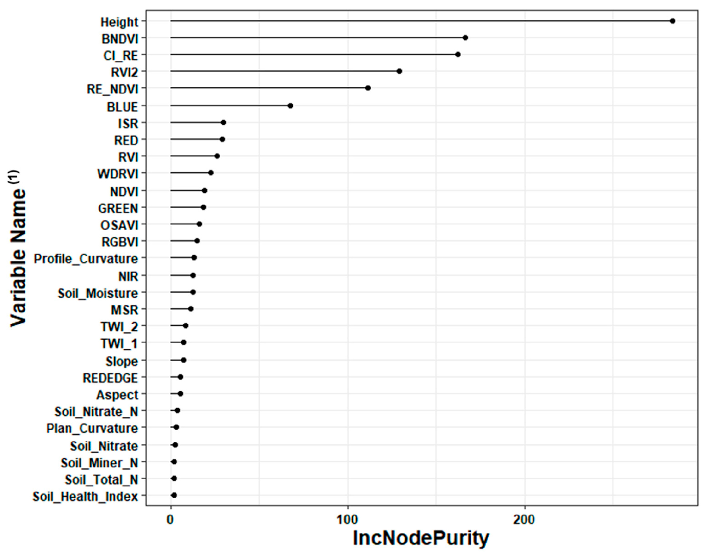(2022) conducted a ten-year field experiment on rice in the Sanjiang Plain of Northeast China (2008–2018, including 30 plot experiments and 13 farmer field trials) to systematically compare the diagnostic accuracy of two indirect strategies and one direct strategy for NNI [29]. The results showed that Random Forest achieved the best effect when fusing multi-source data. In independent validation, the Direct NNI prediction strategy yielded the highest diagnostic accuracy (area consistency of 84%, Kappa coefficient of 0.71), outperforming Indirect Strategy I (77%, 0.58) and Indirect Strategy II (81%, 0.67). Based on this model, farmer field trials demonstrated that precision rice management further reduced nitrogen application rates by 23–24 kg/ha compared to regional optimal management, while improving nitrogen partial factor productivity by approximately 23%.

Yang et al. (2026) approached it from a different technical path, combining physical models with deep transfer learning for winter wheat Canopy Nitrogen Density (CND) estimation [30]. The study first employed the N-PROSAIL radiative transfer model to generate 6000 sets of precisely labeled simulated spectral datasets as the source domain. Based on these datasets, a one-dimensional convolutional neural network (SCAR-CNN) was pre-trained, incorporating channel attention mechanisms and residual connections, followed by fine-tuning using limited field-measured hyperspectral data. Results from two-year field trials demonstrated that the hybrid framework achieved significantly superior CND estimation accuracy (R² = 0.81, RMSE = 0.14) compared to traditional look-up table inversion (R² = 0.45, RMSE = 0.39) and unpre-trained deep learning models (R² = 0.78, RMSE = 0.24). More importantly, the model exhibited validation R² values ranging from 0.43 to 0.89 across different growth stages (from jointing to grain filling), and maintained R² values between 0.43 and 0.88 under varying nitrogen fertilizer concentrations (0 kg/hm², 186 kg/hm²,373 kg/hm²,560 kg/hm²). Even when applied to drone-based hyperspectral data during the grain filling stage, the estimation R² remained at 0.68. Both studies revealed a consistent pattern: prior knowledge from physical models effectively constrains and supplements data-driven models, while transfer learning serves as a bridge connecting “abundant but insufficiently realistic” simulated data with “realistic but inadequate” measured data.

At the sensor level, the comparison between active canopy sensors (GreenSeeker, Crop Circle) and chlorophyll meters (SPAD) is also noteworthy. Ji et al. (2020) showed in a study on pak choi that the correlation coefficients of GreenSeeker’s NDVI and RVI with aboveground biomass reached 0.698–0.967 and 0.642–0.951 [134], respectively, whereas the correlation between SPAD and biomass was insignificant in early growth stages, and although it improved in later stages, it remained lower than the sensor indices. Incorporating growth period days into the model improved the estimation accuracy of biomass by sensor indices by 19–85%, indicating that growth progress information is an unignorable covariate in nitrogen diagnosis.

4.2. Forest and Urban Green Space Structure and Biomass Estimation

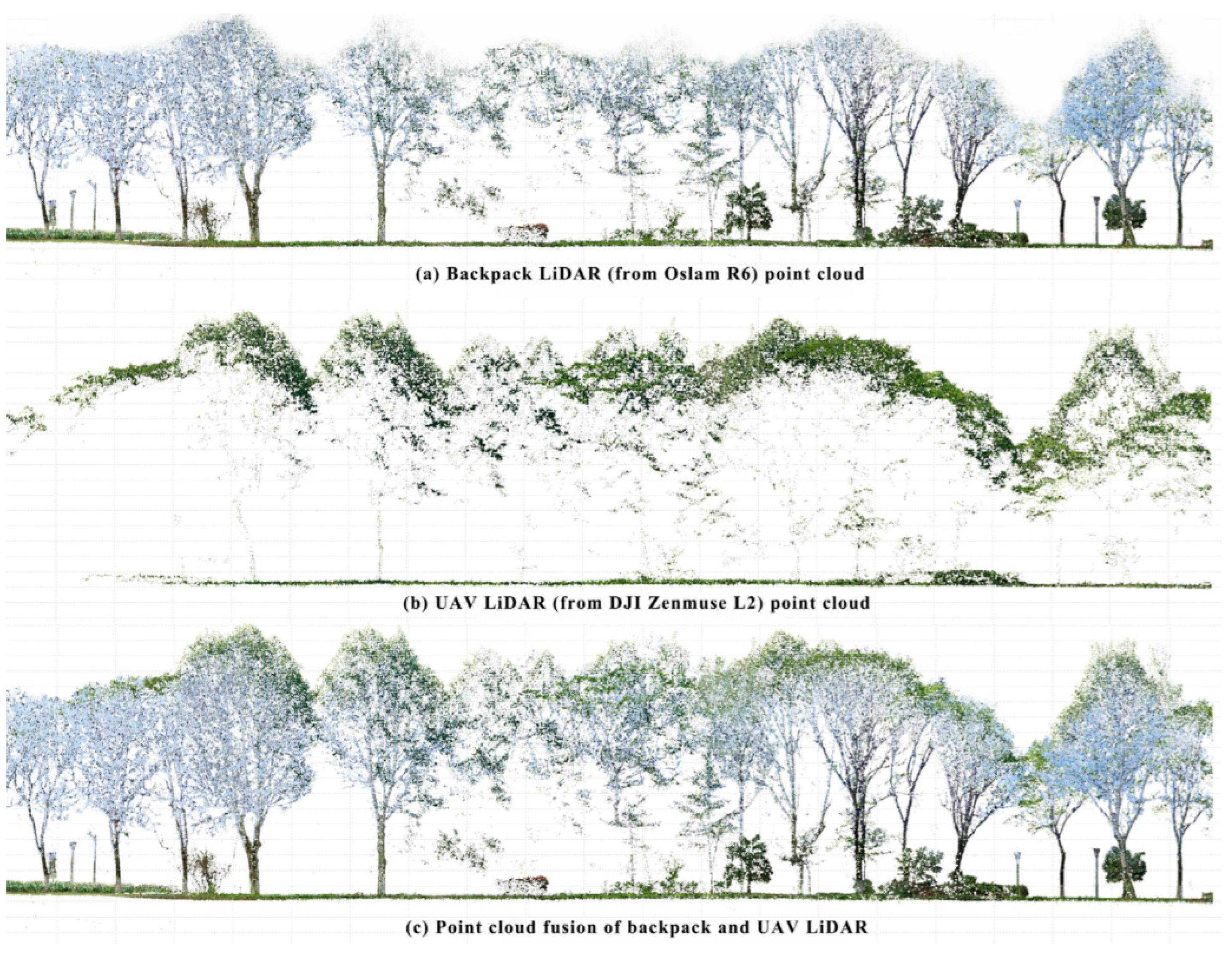
Accurate acquisition of forest structural parameters serves as the foundation for carbon stock estimation and forest health assessment. Traditional plot surveys are particularly arduous in stands with diverse tree species and complex structures, whereas UAV platforms equipped with LiDAR and photogrammetry techniques offer new avenues to resolve this challenge [135].

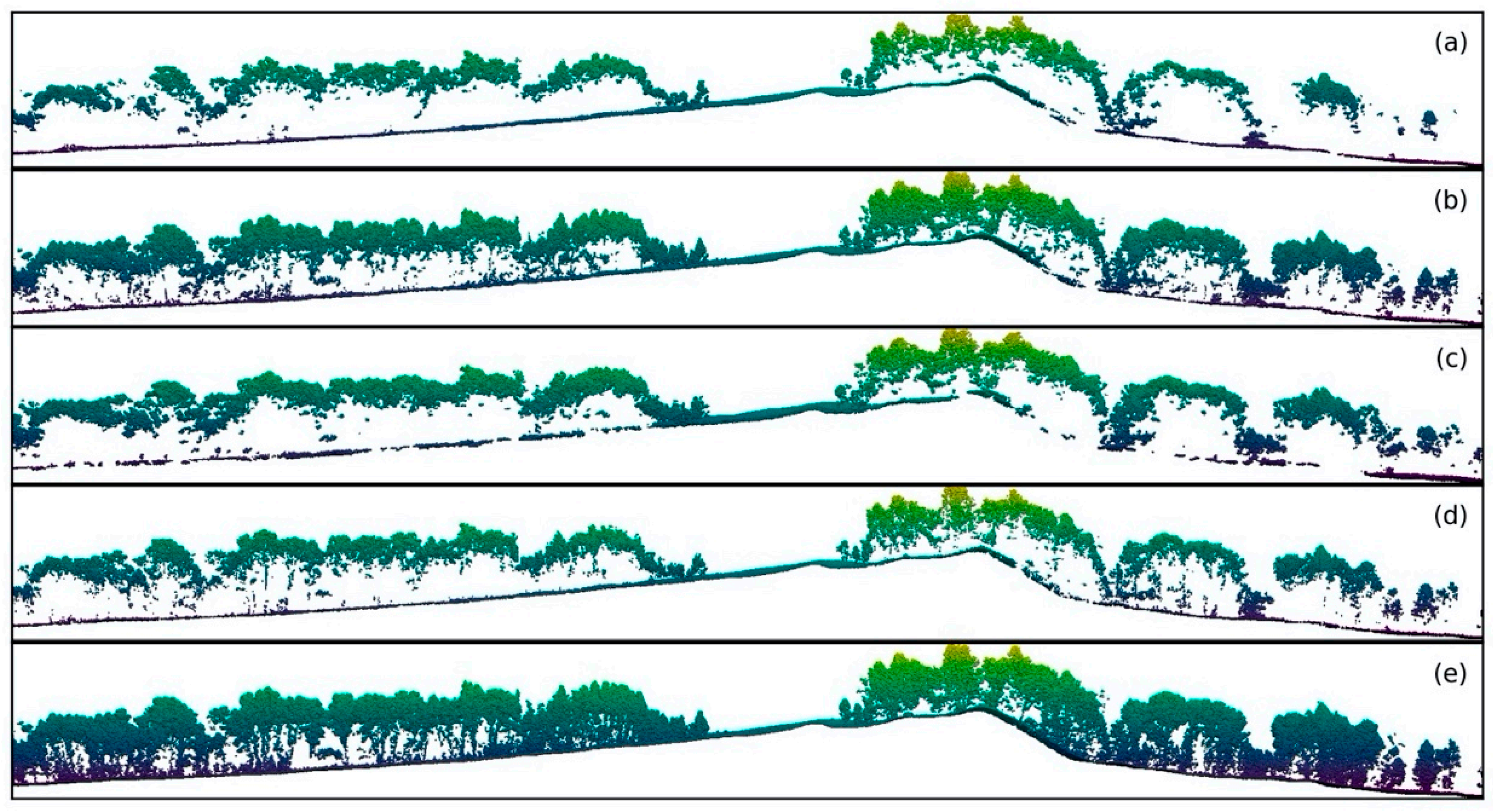
Subedi and Zurqani (2026) conducted a systematic study on an 8.1-hectare pine plantation at the University of Arkansas at Monticello, evaluating the effects of flight speed (10, 15, 20 mph) and image overlap rates (50:50, 60:60, 70:70, 80:80) on the quality of SfM photogrammetry results and LiDAR point cloud data accuracy for tree height estimation [57]. The study used 920 field-measured trees as validation samples. Results demonstrated that image overlap had a significantly stronger impact than flight speed: increasing overlap from 50:50 to 80:80 more than doubled flight time and sextupled the number of images required. For tree height estimation accuracy, LiDAR performed optimally at 10 mph and 80:80 overlap rates (R² ≈ 0.89, RMSE < 1.5 m, deviation < 0.5 m), maintaining high consistency across all flight configurations. In contrast, drone-based SfM achieved only optimal performance under these conditions (R² ≈ 0.60, RMSE = 4.5 m, deviation = 4.3 m), with all estimates showing systematic underestimation. The substantial performance gap between LiDAR and SfM photogrammetry for tree height estimation (R² = 0.89 vs. 0.60) is rooted in fundamental physical differences in their data acquisition mechanisms, which deserve explicit elucidation.

SfM photogrammetry relies entirely on optical image matching—it reconstructs three-dimensional structure by identifying and matching homologous features across overlapping RGB or multispectral images. This approach suffers from three inherent limitations when applied to forest canopies. First, illumination sensitivity: SfM requires adequate and stable lighting conditions; shadows cast by upper canopy elements create radiometric discontinuities that disrupt feature matching in the understory. Second, texture dependency: SfM algorithms require distinct visual texture to establish correspondences between images. In dense, closed-canopy forests where adjacent tree crowns form a continuous, homogeneous green surface, the lack of discriminative features leads to matching failures. Third and most critically, the inability to penetrate the canopy: SfM reconstructs only the visible surface of the canopy—the uppermost layer that is directly illuminated and observed from above. The lower canopy strata and forest floor remain entirely occluded, making it impossible for SfM to capture the vertical structure beneath the crown surface. This explains why SfM systematically underestimated tree height in the studies reviewed: the algorithm effectively measured the top of the canopy surface rather than the true ground-to-top tree height.

LiDAR, by contrast, overcomes all three limitations through its active ranging principle. By emitting laser pulses and recording their return times, LiDAR measures distance directly rather than relying on passive image matching. Its multiple-return capability is particularly critical for forest applications: a single laser pulse can generate multiple discrete returns as it penetrates through canopy gaps and reflects off successive surfaces—the top of the crown, intermediate branches, sub-canopy vegetation, and finally the ground. Even in dense forest stands, a substantial proportion of pulses find gaps sufficient to reach the lower canopy and ground, enabling the reconstruction of the full vertical profile from the Digital Terrain Model (DTM) to the canopy surface. This provides a direct measurement of tree height as the difference between the canopy surface and the ground elevation. Furthermore, LiDAR is independent of illumination conditions, operating reliably day and night without being affected by shadows or varying solar angles, and is robust to texture variations because it does not rely on image feature matching.

Additional advantages of LiDAR over SfM include: (i) direct measurement of ground topography: LiDAR pulses that reach the forest floor enable accurate DTM generation even under dense canopies, whereas SfM struggles to reconstruct ground elevation in forested areas due to occlusion; (ii) vertical canopy profiling: LiDAR returns distributed along the vertical axis allow calculation of height percentiles (P10, P25, P50, P75, P95), gap fraction profiles, and foliage height diversity indices, which are simply unattainable with photogrammetric point clouds that concentrate exclusively on the outer canopy envelope; and (iii) biomass estimation via structural metrics: LiDAR-derived metrics such as mean height, height percentiles, and canopy cover fraction have been shown to correlate more strongly with aboveground biomass than spectral vegetation indices derived from optical imagery, as demonstrated in Thinley et al.’s (2025) [53] mixed-species urban forest study, where adding Sentinel-2 spectral indices did not improve AGB estimation beyond the LiDAR-based CHM alone.

That said, SfM retains complementary advantages that should not be overlooked. It offers lower hardware cost (standard RGB cameras versus specialized LiDAR instruments), higher spatial resolution texture information (true-color orthomosaics), and spectral information across multiple bands when multispectral cameras are used. For open-canopy or sparsely vegetated areas, SfM can achieve comparable accuracy to LiDAR at a fraction of the cost. Therefore, the choice between LiDAR and SfM should be guided by the specific application requirements: LiDAR is the preferred tool for closed-canopy forest structural assessment, understory characterization, and precise terrain modeling, while SfM offers a cost-effective alternative for open vegetation types and applications where spectral texture is equally important as structure. LiDAR point density increased with higher overlap rates, reaching its peak at 10 mph and 80:80 overlap (437.8 points/m²—over three times that of 50:50); however, percentiles of height (P25, P50, P75, P95) showed no significant differences among configurations, indicating limited improvement in canopy structure parameters beyond certain density thresholds. This study provides a quantitative basis for optimizing flight parameters in drone-based forest surveys.

Thinley et al. (2025) selected a 9-hectare urban arboretum at Griffith University’s Logan campus in Queensland, Australia (56 tree species, stand age approx. 10 years), as the research subject to evaluate the capability of LiDAR-generated CHM to estimate tree height and aboveground biomass (AGB) in a mixed-species urban forest [53]. Using 287 field-measured trees as a baseline, they found that the Pearson correlation coefficient between CHM and measured tree height was 0.85, and the linear regression R² was 0.73 (Tree Height = 1.94 + 0.85 × CHM). For AGB, the log-linear regression R² of CHM was 0.43. Incorporating Sentinel-2 satellite-derived NDVI, EVI, and LAI into the model did not significantly improve individual tree AGB estimation accuracy, indicating that high-resolution LiDAR structural information carries more informative value than medium-resolution optical imagery in a mixed-species urban forest. All key statistical indicators from this study are consolidated and summarized in

Table 6. Summary of LiDAR Urban Forest Tree Height & Aboveground Biomass (AGB) Estimation Metrics.

Prediction Target	Statistical Indicators	Value	Data Source
Tree Height	Pearson Correlation Coefficient (r)	0.85	Thinley et al. (2025) [53]
Tree Height	Linear Regression R2	0.73	Thinley et al. (2025) [53]
Tree Height	Regression Equation	Tree Height = 1.94 + 0.85 × CHM	Thinley et al. (2025) [53]
Aboveground Biomass (AGB)	Log Regression R2	0.43	Thinley et al. (2025) [53]

.

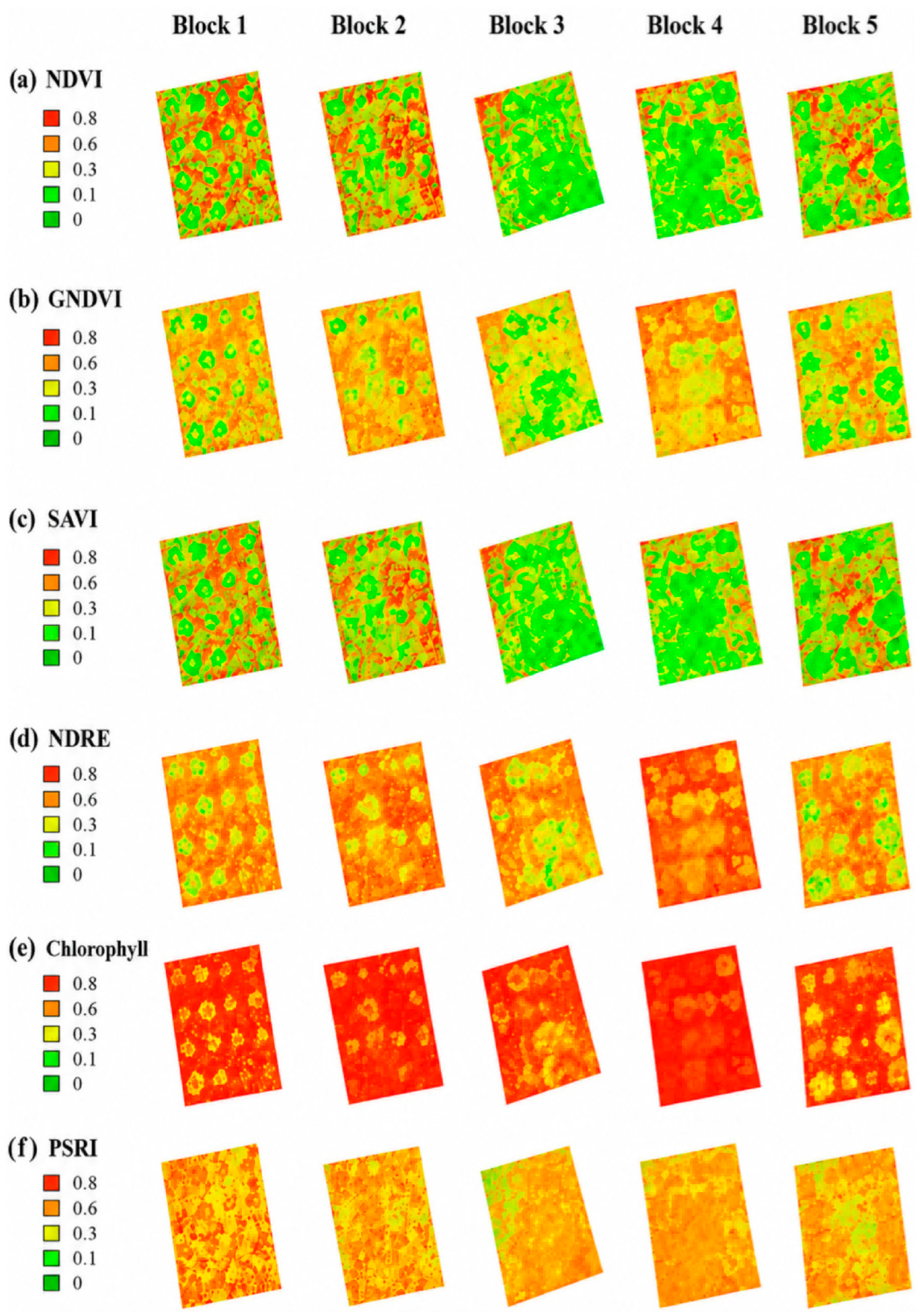
Ferreira et al. (2025) jointly applied hyperspectral and LiDAR data to evaluate the ecological management of tropical seasonal forests [39]. Across 18 plots in Vassununga State Park, São Paulo, Brazil, they collected UAV hyperspectral (400–1000 nm) and LiDAR data in both the dry and wet seasons. The study revealed that during the dry season, pigment-sensitive vegetation indices (PARS, GMI1, SR3) exhibited a moderate-to-large negative response to liana removal (Cohen’s d = −0.595 for PARS), reflecting a significant drop in canopy greenness following the removal of evergreen lianas; conversely, the effect of wet season indices (DD, OSAVI2, MSAVI) was negligible (Cohen’s d < 0.2), as both trees and lianas fully flush their leaves under resource-abundant conditions, masking differences. Wavelength-wavelength correlation analysis localized the signals with the strongest treatment effects to the red-edge region (approx. 700 nm). Regarding structural parameters, liana removal caused a small-to-moderate reduction in understory LAI (dry season Cohen’s d = −0.481), whereas canopy height changed minutely (Cohen’s d ranged from only −0.052 to 0.085). In alignment with the vegetation index-based assessment framework for forest canopy status, the spatial distribution patterns of six representative vegetation and biochemical indices across five experimental blocks are visualized in Figure 4, which can intuitively reflect the spatial heterogeneity of vegetation growth conditions within the plots.

4.3. Stress Monitoring and Disaster Warning

The early identification of vegetation stress and disaster warning represent crucial directions for precision management, involving aspects such as moisture stress, mechanical damage (lodging), fire smoke, and life sign detection [136,137,138].

From a plant monitoring perspective, it is essential to distinguish between two broad categories of vegetation stress: biotic stress and abiotic stress, as their causes, temporal dynamics, spectral signatures, and management responses differ fundamentally. Biotic stress arises from living organisms—including pathogens (fungi, bacteria, viruses), insect pests, parasitic plants, and competing weeds—and typically exhibits localized, spatially clustered, and progressively spreading patterns. Its detection often relies on subtle changes in leaf pigments, cell structure, and canopy temperature, with hyperspectral and thermal sensors playing key roles in early identification. Abiotic stress, by contrast, originates from non-living environmental factors such as drought, waterlogging, extreme temperatures, nutrient deficiency, salinity, mechanical damage (lodging), fire, and air pollution. Abiotic stress tends to manifest at broader spatial scales following environmental gradients and may induce rapid physiological responses. While the visual symptoms of biotic and abiotic stresses (e.g., chlorosis, necrosis, wilting, stunting) can overlap considerably, their underlying mechanisms and management implications are distinctly different: biotic stress requires targeted intervention (e.g., fungicide application, pest control), whereas abiotic stress necessitates adjustment of environmental or agronomic conditions (e.g., irrigation, fertilization, density regulation, or structural reinforcement). Therefore, accurate stress discrimination is not merely a taxonomic exercise but a prerequisite for informed decision-making in precision agriculture and forest health management. The following subsections review representative case studies spanning both categories, with emphasis on moisture stress and lodging risk as abiotic stressors, fire smoke detection as an environmental hazard indicator, and life sign detection as an emerging application of radar sensing.

Regarding moisture stress monitoring, Tapia-Zapata and Zude-Sasse (2026) utilized a dual-wavelength near-infrared LiDAR scanner (1320 nm and 1450 nm) to perform leaf water evaluation on apple tree canopies [139]. The study chose six pots of 7-year-old “Gala” apple trees as subjects, setting up two treatment groups—well-irrigated and drought-stressed—while simulating a leaf surface free water spraying scenario. After separating leaf and woody structures using a semi-automatic algorithm, they calculated the normalized returned signal intensity (I Norm) and the Normalized Difference NIR index (NDNIR). The results showed that well-irrigated and drought-stressed canopies exhibited only minute differences across all LiDAR-derived variables. Wasserstein distance statistics indicated that the mean distribution shift before and after spraying was 14.3 for I Norm and 19.8 for NDNIR, demonstrating that the strong absorption characteristics of water at 1450 nm render this band highly sensitive to leaf surface free water. This study indicates that LiDAR is insufficiently sensitive to changes in internal physiological leaf water content but possesses potential for detecting leaf surface free water (such as dew or irrigation residues), providing a new technical pathway for orchard microclimate management and disease prediction.

In terms of lodging risk prediction, Dong et al. (2023) utilized the Crop Circle ACS-430 active canopy sensor to collect canopy reflectance data during the maize V8 growth stage, combining it with variables such as planting density, nitrogen application rate, growing degree days, and cumulative precipitation to construct an early prediction model for maize stem lodging risk [140]. Based on the maize stem lodging process model developed by Berry et al. 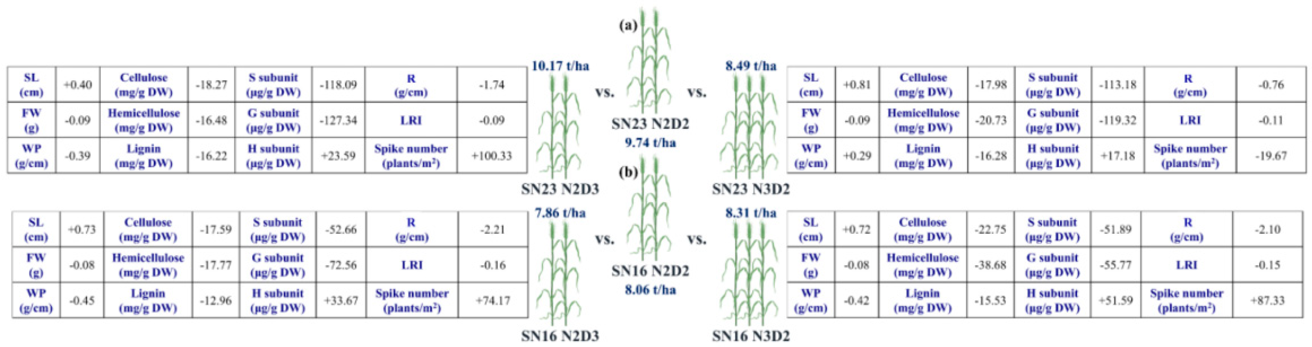(2021), the study used failure wind speed as a quantitative indicator for lodging risk [141,142,143]. Liu et al. (2025) further investigated the combined effects of nitrogen application and planting density on grain yield and lodging resistance in winter wheat [144]. A two-year field experiment was conducted using two wheat cultivars with contrasting lodging resistance under three nitrogen application rates (120, 240, and 360 kg ha⁻¹) and four planting densities (75, 225, 375, and 525 plants m⁻²). Increasing nitrogen application and planting density generally reduced the lodging resistance index (LRI), whereas grain yield initially increased and subsequently decreased, indicating a clear trade-off between productivity and lodging resistance. The lodging-resistant cultivar SN23 showed both higher grain yield and stronger lodging resistance than the lodging-sensitive cultivar SN16. Among the tested treatments, a nitrogen application rate of 240 kg ha⁻¹ combined with a planting density of 375 plants m⁻² provided a favorable balance between yield and lodging resistance. These results demonstrate that optimizing nitrogen input and planting density can serve as a proactive agronomic strategy for reducing lodging risk while maintaining high crop productivity. The trade-off between grain yield and lodging resistance under different nitrogen–density combinations is illustrated in Figure 5.

For fire and smoke detection, Schenkel et al. (2024) [28] conducted a systematic study. Under laminar flow conditions in an EN54-7 standard smoke wind tunnel, as the smoke particle volume fraction increased linearly from 0 to 0.465 ppm, the phase change of the radar signal exhibited a highly consistent upward trend with MIREX optical extinction measurements [28]. In real fire tests, the phase change patterns generated by two standard test fires—polyurethane foam (TF4) and n-heptane (TF5)—corresponded well with different stages of the combustion process: ignition, fully developed burning, and extinguishment. The phase change amplitude reached 62° for TF5 and 45.55° for TF4, a difference correlated with the heat release rates of the two fuels [145,146]. Test data for the millimeter-wave radar phase response under smoke wind tunnel and real fire scenarios are summarized in

Table 7. Phase Response Test Data of Millimeter-Wave FMCW Radar in Smoke Wind Tunnel/Fire Scenarios.

Test Scenario	Measurement Parameter	Value/Change	Data Source
Smoke Wind Tunnel (Laminar)	Smoke Particle Volume Fraction Range	0 → 0.465 ppm	Schenkel et al. (2024) [28]
Smoke Wind Tunnel (Laminar)	Radar Phase Change	Radar Phase Change Amplitude	Schenkel et al. (2024) [28]
TF5 (n-Heptane Fire)	Radar Phase Change Amplitude	62°	Schenkel et al. (2024) [28]
TF4 (Polyurethane Foam Fire)	Radar Phase Change Amplitude	45.55°	Schenkel et al. (2024) [28]

. The study also explained the physical mechanism from the perspective of dielectric theory: water vapor and CO₂ generated by combustion alter the refractive index of the air mixture; according to the Debye equation and the Lorentzian line shape model, water vapor possesses significant polar molecular resonance absorption features in the millimeter-wave frequency band, and its refractive index change can reach the order of 10⁻⁶, sufficient to be captured by high-sensitivity phase measurements. This finding demonstrates the unique advantage of millimeter-wave radar in environments with extremely low visibility (smoke, dust)—conditions where traditional optical and thermal imaging methods often fail, yet radar signals remain unaffected [147,148].

In terms of life sign detection, Sato et al. (2024) achieved in-vehicle child presence detection utilizing a 60 GHz band MIMO-FMCW radar combined with machine learning methods [77]. The study collected data across two vehicle models, the Toyota Prius (two rows of seats) and the Nissan Serena (three rows of seats), as shown in

Table 8. Performance of Millimeter-Wave Radar In-Vehicle Occupancy Detection Models.

Vehicle Model	Classification Task	Model	Accuracy	Feature Count	Data Source
Toyota Prius (Two Rows)	Three-class (Adult/Infant/Empty)	XGBoost	≈100%	74	Sato et al. (2024) [77]
Toyota Prius (Two Rows)	Three-class (Adult/Infant/Empty)	DNN	≈100%	74	Sato et al. (2024) [77]
Nissan Serena (Three Rows)	Binary (Infant/Empty Seat)	XGBoost	≈100%	74	Sato et al. (2024) [77]
Nissan Serena (Three Rows)	Binary (Infant/Empty Seat)	DNN	≈100%	74	Sato et al. (2024) [77]

, obtaining range information through Range-FFT and estimating the angle of arrival using the Capon algorithm to generate range-azimuth heatmaps, from which 74 categories of 1D features were extracted (including power maximums, azimuth angles, distances, and their temporal statistics for each seat area). In the three-class classification task (adult/infant/empty seat) for the two-row seat model, both XGBoost and DNN models achieved near 100% classification accuracy; the binary classification task (infant/empty seat) for the three-row seat model was similarly near 100%. One of the innovations of this study lies in introducing power temporal correlation as a feature to detect the periodic respiration of infants—even though an infant’s radar cross-section is much smaller than an adult’s, the periodic chest wall movement caused by breathing can still leave identifiable signals in the power time-series [149,150]. To further enhance model explainability and deployment efficiency, researchers approximated XGBoost into an explainable decision tree, reducing the model evaluation time from the millisecond level to the sub-millisecond level and significantly downsizing the model volume by removing redundant branches and optimizing evaluation algorithms. This work demonstrates a complete technical path from a “high-precision black box” to an “explainable lightweight model,” offering a valuable reference for the practical deployment of in-vehicle safety systems.

To provide a synthetic overview of the quantitative benefits of multi-source data fusion,

Table 9. Performance Comparison: Single-Sensor versus Multi-Source Fusion Approaches.

Application	Single-Sensor Performance	Fusion Performance	Improvement	Source
LAI Estimation (Forest)	R2 = 0.72, RMSE = 2.12	R2 = 0.73, RMSE = 0.54	RMSE ↓ 74.5%	Zeng et al. (2026) [21]
Tree Height Estimation	R2 ≈ 0.60, RMSE = 4.5 m (SfM)	R2 ≈ 0.89, RMSE < 1.5 m (LiDAR)	R2 ↑ 48.3%, RMSE ↓ 66.7%	Subedi and Zurqani (2026) [57]
Canopy Nitrogen Density	R2 = 0.45, RMSE = 0.39 (LUT)	R2 = 0.81, RMSE = 0.14 (TL)	R2 ↑ 80.0%, RMSE ↓ 64.1%	Yang et al. (2026) [30]
Rice NNI Diagnosis	Accuracy: ~70% (sensor only)	Accuracy: 84%, Kappa = 0.71	Accuracy ↑ ~14–20%	Lu et al. (2022) [29]
Maize Lodging (Wind Speed)	R2 = 0.43, RMSE = 0.79 m/s	R2 = 0.69, RMSE = 0.58 m/s	R2 ↑ 60.5%, RMSE ↓ 26.6%	Dong et al. (2023) [46]
Maize Lodging (Failure Moment)	R2 = 0.67, RMSE = 3.73 Nm	R2 = 0.83, RMSE = 2.69 Nm	R2 ↑ 23.9%, RMSE ↓ 27.9%	Dong et al. (2023) [46]

Note. ↑ indicates an increasing trend, and ↓ indicates a decreasing trend.

summarizes key performance metrics from representative studies reviewed in this paper, comparing single-sensor (or single data type) approaches with multi-source fusion strategies.

5. Current Challenges and Future Outlook

Although multi-source sensing technologies and advanced modeling methods have made significant progress in the field of vegetation monitoring, moving from laboratory research to operational application still faces numerous bottlenecks [98]. Based on a review of existing challenges, this chapter discusses potential future research directions.

5.1. Current Challenges

Data Heterogeneity and Standardization: Vegetation monitoring involves multiple sensors such as optical, LiDAR, and radar across different platforms like satellites, UAVs, and ground systems, which exhibit fundamental differences in spatial resolution, spectral configuration, and viewing geometry. Even for LiDAR data alone, variations in the beam divergence angle across different systems can cause an LAI estimation bias of up to 42% (Zeng et al., 2026) [21], indicating that differing sensor specifications generate systematic errors. Currently, a lack of unified data acquisition standards and metadata specifications makes cross-study and cross-regional comparison and integration extremely difficult.

To move beyond problem identification, three complementary strategies are emerging to mitigate data heterogeneity. First, generative adversarial networks (GANs) and other domain translation techniques offer a promising data-level solution. Recent studies have demonstrated that CycleGAN and conditional GAN architectures can effectively translate imagery between different sensor modalities (e.g., Sentinel-2 to Landsat, or UAV-LiDAR to airborne-LiDAR), generating synthetic data that mimics the spectral or structural characteristics of target sensors while preserving the biophysical content. This approach can alleviate the scarcity of multi-sensor paired training data and enable cross-sensor model transfer. Second, the development of unified data standards and metadata specifications is urgently needed. Initiatives such as the FAIR (Findable, Accessible, Interoperable, Reusable) data principles and community-agreed formats for LiDAR point clouds (e.g., LAS/LAZ with standardized extra dimensions) and hyperspectral imagery (e.g., ENVI-compliant metadata) could facilitate cross-study integration. Third, the establishment of community reference datasets—carefully curated ground-truth sites with concurrent multi-sensor acquisitions (optical, LiDAR, radar) and rigorous field measurements—would serve as a ‘gold standard’ for benchmarking and calibrating heterogeneous data. Such reference sites, analogous to the FLUXNET network for flux measurements, would enable systematic quantification and correction of sensor-specific biases. Collectively, these strategies provide a roadmap from the current ad hoc handling of heterogeneity toward a more principled and interoperable monitoring framework.

Model Generalization Capability and Physical Explainability: The “black-box” nature of machine learning models limits their trustworthiness in critical decision-making scenarios [101]. Purely data-driven methods lack physical constraints and may generate inversion results that contradict known physical laws. In forest health monitoring, domain shift severely restricts the cross-regional generalization ability of deep learning models. Physics-Informed Neural Networks (PINNs) attempt to embed radiative transfer models into neural network architectures to maintain physical consistency, but such methods are currently still in the concept-validation stage and remain far from operational application.

Small-Sample Problem and Annotation Costs: Acquiring high-quality field-measured data is the most expensive phase in vegetation remote sensing modeling. The study by Lu et al. (2022) spanned ten years yet yielded only nearly 2000 samples, which remains limited for deep learning models [29]. The research by Yang et al. (2026) showed that even when using transfer learning, a sample size of 384 over two years saw its R² drop from 0.81 to 0.50 in cross-year validation, demonstrating that the small-sample problem is particularly acute in cross-year scenarios [30]. Biodiverse regions especially lack sufficient field calibration data.

The Transformation Gap from Data to Decision Support: Most studies stop at the accuracy verification stage of parameter inversion, rarely involving how to establish quantitative links between inversion results and specific agronomic or management measures. The work of Lu et al. (2022) represents one of the few attempts to convert NNI diagnosis into nitrogen fertilizer recommendations, but the recommendation model still relies on regional average parameters and has not achieved field-level personalized decision-making [29]. The transformation chain from academic achievements to field tools remains incomplete.

To move beyond accuracy validation toward actionable decision support, physics-based information models are increasingly being embedded into operational Decision Support Systems (DSS). For instance, the AgriCarbon-EO tool assimilates high-resolution Sentinel-2 optical data into the PROSAIL radiative transfer model and the SAFYE-CO2 crop model, delivering 10 m resolution maps of yield, biomass, and carbon/water budgets at regional scales [151]. Similarly, the N-PROSAIL model has been coupled with deep transfer learning to achieve robust canopy nitrogen density estimation in winter wheat, providing a foundation for in-season nitrogen fertilizer recommendations [30]. In another example, radiative transfer model inversion has been used to estimate green leaf area index (gLAI) and chlorophyll content from hyperspectral reflectance, supporting site-specific nitrogen fertilization management at the within-field scale. These examples illustrate that the technical pathway from physical model inversion to management prescriptions is technically feasible.

However, several key barriers impede the translation of research-grade models into practical DSS tools that are widely adopted by farmers and agronomists. First, scaling challenges arise because most physics-based models are calibrated and validated under controlled experimental conditions, yet their performance often degrades when applied across diverse agroecological zones, soil types, and climate regimes. Second, end-user interface design remains a critical bottleneck: the complexity of biophysical models—particularly when their individual sub-modules are integrated—makes them difficult for end-users to understand and operate. Certified crop advisors have been shown to favor systems that augment rather than replace professional judgment, valuing editable workflows, local calibration, and field verification over black-box precision. Third, integration with existing agronomic software poses substantial technical hurdles, including limited interoperability between monitoring hardware and software, and the absence of standardized data formats linking field observations with accounting and decision frameworks. Addressing these barriers requires not only algorithmic advances but also participatory design processes that co-create tools with end-users, ensuring that DSS are trusted, equitable, and context-sensitive.

Algorithm and System Complexity: The training and deployment of deep learning models demand high computational resources, while edge devices possess limited computing capacity. Sato et al. (2024) achieved model lightweighting by approximating XGBoost into explainable decision trees, but at the cost of sacrificing some accuracy [77]. The preprocessing, registration, and fusion of multi-source data involve complex workflows, requiring high professional expertise from operators, which limits the grassroots promotion of these technologies.

Computational Load and Deployment Feasibility: Beyond algorithmic complexity, the practical deployment of deep learning models and RTM inversion frameworks on edge devices, UAVs, or real-time agricultural monitoring hardware faces severe computational constraints. For instance, the SCAR-CNN architecture, while achieving high accuracy for canopy nitrogen density estimation, requires substantial memory and floating-point operations that exceed the capabilities of typical onboard embedded systems. Similarly, 3D LiDAR point cloud processing—involving registration, filtering, classification, and feature extraction—demands significant computational resources that are challenging to satisfy in real-time on UAV platforms with limited power budgets and processing capacity. RTM inversion via look-up tables or iterative optimization, although physically interpretable, becomes computationally prohibitive when applied at large scales or when requiring near-real-time responses. These constraints are particularly acute in precision agriculture scenarios where decisions must be made within narrow time windows (e.g., variable-rate nitrogen application during crop growth stages), and where UAVs have limited battery life and onboard processing power. The gap between research-grade model performance and edge-deployable feasibility thus represents a critical bottleneck that must be addressed for the successful translation of academic advances into operational tools.

5.2. Future Research Outlook

Before outlining future technological directions, several unresolved scientific issues merit explicit discussion. First, current radiative transfer models (RTMs) remain fundamentally constrained by their one-dimensional turbid-medium assumptions, which treat canopies as horizontally homogeneous layers. While this simplification works well for uniform agricultural crops, it systematically fails in structurally complex scenes such as forests, mixed-species stands, orchards, and savannahs, where clumping effects, horizontal heterogeneity, multiple-scattering between discrete elements, and contributions from non-photosynthetic components are poorly represented. These limitations cannot be resolved simply by adding new sensor platforms; instead, they call for a paradigm shift toward three-dimensional heterogeneous scene representations that explicitly incorporate crown geometry, branching architecture, and realistic background properties. Second, the development of truly bidirectional hybrid models remains an open challenge. The current emphasis on Physics-Informed Neural Networks (PINNs)—where physical laws regularize data-driven models—should be complemented by the emerging paradigm of Data-Informed Physics Models (DIPMs), in which observational data are used not merely to validate but to refine the parameters, structure, or assumptions of physical models themselves. The integration of these two directions would establish a synergistic framework where physical knowledge and empirical observations mutually inform and correct each other, enhancing both predictive accuracy and interpretability across diverse ecosystems.

“Space-Air-Ground” Integrated Monitoring Network: Constructing a collaborative monitoring system comprising satellites (macro), UAVs (meso), and the ground Internet of Things (micro) can achieve information complementarity through data fusion and data assimilation, breaking through the spatiotemporal coverage limitations of a single platform [106]. Deploying lightweight sensors on under-canopy UAVs offers a new path to acquire understory structural information that is difficult to capture via traditional above-canopy remote sensing.

Advanced AI Fusion Methods: Physics-guided neural networks embed radiative transfer models into network architectures, subjecting models to both data loss and physical laws, thereby improving prediction accuracy under small-sample conditions [107]. Graph Neural Networks (GNNs) provide a new tool for handling spatial dependencies within the canopy. Domain adaptation and domain generalization techniques hold the promise of constructing more universal foundation models by disentangling domain-invariant and domain-specific features.

Model Compression and Lightweight Architectures for Edge Deployment: To bridge the gap between high-accuracy models and resource-constrained deployment platforms, model compression techniques have emerged as a promising research direction. Three primary approaches are gaining traction in vegetation monitoring and remote sensing applications:

Pruning removes redundant or less important parameters from trained neural networks, significantly reducing model size with minimal accuracy degradation. Recent studies have demonstrated that pruning alone can reduce model size by approximately 55–65% with only a 1–3% accuracy drop in UAV-based weed detection tasks. When combined with other compression techniques, pruning enables deep learning models to run efficiently on edge devices such as NVIDIA Jetson platforms.

Quantization reduces the numerical precision of model parameters (e.g., from 32-bit floating point to 8-bit integers), thereby decreasing memory footprint and accelerating inference. Quantization alone has achieved approximately 35–50% model size reduction, and combined pruning and quantization can yield up to 75% model size reduction while maintaining over 90% accuracy.

Knowledge Distillation trains a compact “student” model to mimic the behavior of a larger, more accurate “teacher” model. This approach has proven particularly effective in remote sensing applications: for example, a distilled student model derived from SAM2 reduced parameters by 97% (from 222.98 M to 6.68 M) while preserving more than 99% of the teacher network‘s accuracy for high-resolution remote sensing semantic segmentation. In change detection tasks, knowledge distillation has enabled lightweight models with performance comparable to large models, making onboard processing feasible for disaster emergency response.

Beyond these techniques, the development of lightweight architectural designs—such as depth-wise separable convolutions, MobileNet, EfficientNet, and specialized lightweight backbones—offers additional pathways for reducing computational demands while maintaining predictive performance. For LiDAR point cloud processing, real-time transmission and rendering technologies incorporating lossy compression strategies have demonstrated the ability to process millions of point cloud data per second on UAV mobile controllers. Future research should prioritize hardware-aware model design, where compression strategies are co-optimized with the specific constraints of target deployment platforms (e.g., UAV onboard computers, field-deployable edge devices, or satellite processors), to facilitate the operational translation of vegetation monitoring frameworks.

Beyond model compression, the integration of lightweight vision models specifically designed for autonomous platforms—such as UAVs and ground-based robotic systems—warrants particular attention in precision forestry and agriculture. Unlike general-purpose compression techniques, these lightweight architectures (e.g., MobileNet, EfficientNet, YOLO variants, and Vision Transformers with linear complexity) are optimized for real-time inference under strict power and latency constraints. Their deployment enables onboard processing for tasks such as real-time obstacle avoidance, targeted spraying, and early stress detection without relying on cloud connectivity, which is especially valuable in remote or connectivity-limited field environments. Future research should prioritize hardware-software co-design, where model architectures are jointly optimized with specific edge accelerators (e.g., NVIDIA Jetson, Google Coral, or neuromorphic chips) to maximize operational efficiency.

Cloud Platforms and Digital Twins: Cloud computing platforms provide the infrastructure for storing, processing, and sharing massive remote sensing data [108]. Digital twin technology, by constructing virtual mirrors of physical entities, enables a full-chain service of “status perception → scenario deduction → management decision”. Establishing open data-sharing and model-deployment platforms is a key step in driving technology from research to application.

New Sensors and Low-Cost Solutions: Solid-state LiDAR and MEMS scanning technologies drive system miniaturization and low-cost development. Zeng et al. (2026) demonstrated that low-cost LiDAR can still achieve acceptable LAI estimation accuracy through proper calibration [21]. Software-defined radio combined with open-source frameworks provides a new approach to constructing reconfigurable low-cost radars. These technological advancements are expected to lower technical barriers and promote precision monitoring in resource-constrained regions.

Cross-Regional and Cross-Crop Model Transfer: Constructing large-scale open datasets covering multiple crops, ecological zones, and years will support foundation model pre-training [110]. Meta-learning and few-shot learning are expected to enable models to adapt rapidly to new scenarios using only a minimal amount of annotated samples. Yang et al. (2026) showed that the transfer learning model maintained high accuracy when migrating from a ground platform to a UAV platform (R² = 0.68 in the filling stage), proving the feasibility of cross-platform migration, although multi-regional generalization requires further investigation [30].

5.3. Conclusions

This review has systematically surveyed recent advances in multi-source sensing technologies and intelligent modelling methods for vegetation monitoring, covering agricultural crops, forest ecosystems, and mixed vegetation types. The physical principles and complementary nature of passive optical hyperspectral remote sensing, active LiDAR structural detection, and microwave/millimetre-wave radar have been elucidated, demonstrating that no single sensor can fully characterise the complexity of vegetation canopies. Optical sensors excel at retrieving biochemical constituents (chlorophyll, nitrogen, water) through narrow-band spectral signatures, whereas LiDAR provides precise three-dimensional structural information independent of illumination, and radar offers all-weather sensitivity to dielectric properties and moisture dynamics. The synergistic use of these technologies, when coupled with appropriate spatial and temporal alignment strategies, substantially enhances monitoring capabilities across scales.

From a methodological perspective, three complementary modelling paradigms have been examined. Physics-based radiative transfer models (e.g., PROSAIL, N-PROSAIL, DART) provide physically interpretable and generalisable simulations but face ill-posed inversion problems. Data-driven machine learning (Random Forest, XGBoost, deep learning) offers powerful non-linear fitting capabilities but suffers from data scarcity and limited interpretability. Hybrid strategies—particularly physics-data dual-driven frameworks combining radiative transfer model simulations with transfer learning—have emerged as a promising solution, effectively bridging the gap between abundant simulated data and scarce field measurements while maintaining physical consistency.

The successful application of these technologies has been demonstrated across diverse scenarios, including precision nitrogen diagnosis in rice and winter wheat, forest biomass and tree height estimation in both plantation and mixed-species urban forests, early prediction of crop lodging risk, and assessment of vegetation stress from drought, fire, and liana competition. These case studies consistently show that multi-source data fusion significantly improves prediction accuracy and robustness compared with single-sensor approaches.

Nevertheless, several critical challenges persist. Data heterogeneity arising from differing sensor specifications, acquisition geometries, and processing pipelines remains a major obstacle to cross-study integration and model generalisation. The “black-box” nature of deep learning models limits their trustworthiness in decision-making, calling for greater integration of physical constraints and explainable AI techniques. The small-sample problem and high annotation costs constrain model development, particularly in biodiverse and under-studied regions. Furthermore, the translation of research-grade inversion results into operational decision support tools for farmers and forest managers remains incomplete, hindered by scaling issues, user interface complexity, and system integration barriers.

Looking forward, the construction of collaborative “space-air-ground” integrated monitoring networks, combining satellite, UAV, and ground-based IoT sensors, offers a pathway to overcome spatiotemporal coverage limitations. Advanced AI methods, including physics-guided neural networks, graph neural networks for spatial dependency modelling, and domain adaptation techniques, promise to enhance model generalisation and physical consistency. Model compression and lightweight architectures (pruning, quantisation, knowledge distillation) are critical for enabling edge deployment on resource-constrained UAVs and field devices. Finally, the establishment of large-scale open datasets and cloud-based digital twin platforms will be instrumental in accelerating the transition from academic research to practical application, ultimately supporting sustainable agriculture and forest ecosystem management under global environmental change.