Morphology-Aware Wasserstein Distance Loss for Bounding-Box Regression in External Pipeline Coating Inspection

Featured Application

This study targets intelligent screening of external anti-corrosion coating conditions for long-distance pipelines during construction. The proposed morphology-aware Wasserstein distance loss shows improved mean detection sensitivity for coating-condition targets while preserving the inference structure and computational complexity of the YOLOv10n baseline, which provides a basis for future evaluation in mobile-device-based field inspection workflows.

Abstract

Ensuring the integrity of external anti-corrosion coatings is critical to the safe operation of long-distance oil and gas pipelines. Construction-site images contain complex backgrounds, multi-scale targets, and many elongated or weak-boundary coating conditions, challenging conventional bounding-box regression under low-overlap conditions. We constructed a real-site dataset of 1388 images and 1756 annotated instances across six coating-condition categories from long-distance natural-gas pipeline construction sites. Building on YOLOv10n, we formulate a Scale–Aspect Adaptive Normalized Wasserstein Distance (SA-NWD) regression strategy that adjusts the NWD weight according to target scale and aspect ratio during training. Across six random seeds, SA-NWD achieved the highest mean Recall (0.459 vs. 0.437 baseline) and mAP@0.5 (0.451 vs. 0.431), whereas fixed-weight NWD achieved the highest mean mAP@0.5:0.95 (0.251 vs. 0.240 baseline). Ablation results support complementary scale and aspect-ratio guidance. Morphology-grouped analysis showed higher Recall for extremely elongated targets (0.714 vs. 0.659 for fixed-weight NWD), with lower cross-seed standard deviation (±0.027 vs. ±0.101). These results suggest that SA-NWD may benefit high-recall screening of morphologically complex coating conditions, while fixed-weight NWD may provide more stable high-IoU localization; both strategies retain the inference architecture, parameter count, and GFLOPs of the YOLOv10n baseline.

1. Introduction

Oil and gas pipelines constitute a critical infrastructure for long-distance energy transportation. The integrity of external anti-corrosion coatings in oil and gas pipelines is directly related to pipeline service safety, operational stability, and economic efficiency [1,2,3]. During pipeline construction, three-layer polyethylene (3PE) anti-corrosion coatings are prone to surface defects such as mechanical damage, heat-shrink sleeve-edge lifting, disbonding, and closure patch cracking. If these defects are not detected and repaired before pipeline trenching and backfilling, they may cause local coating failure, thereby increasing the risk of pipe body corrosion and safety accidents. Although manual visual inspection is easy to implement on construction sites, it is inefficient, subjective, and difficult to standardize across inspectors and environmental conditions. It is also difficult to meet the requirements for stable recognition of small, elongated, and irregular defects under complex backgrounds [4,5,6,7]. This motivates the development of automated visual inspection methods for pipeline external anti-corrosion coating quality assessment.

In recent years, deep learning, especially convolutional neural networks (CNNs), has shown strong feature representation capability in image feature extraction and object detection tasks [8,9]. Deep learning-based object detection algorithms can generally be divided into two-stage and one-stage methods. Two-stage methods, represented by R-CNN and its improved variants, typically achieve high localization accuracy by first generating region proposals and then performing classification and bounding-box regression [10,11]. For example, Libra R-CNN improves detection performance by alleviating imbalance in samples, features, and objective functions [12]. However, such methods involve relatively complex computational pipelines and relatively slow inference speed, which limits their application in industrial inspection scenarios requiring real-time performance. In contrast, one-stage detectors, such as Single Shot MultiBox Detector (SSD) [13] and the You Only Look Once (YOLO) series [14,15,16], perform object localization and category prediction through a single forward pass, offering advantages in detection speed, structural simplicity, and deployment convenience. Among them, YOLOv10 further targets real-time end-to-end detection by using a Consistent Dual Assignment strategy to reduce dependence on non-maximum suppression post-processing. Combined with an accuracy–efficiency co-designed architecture, YOLOv10 offers a favorable accuracy–latency trade-off in general object detection [17], making it a reasonable baseline to investigate for this industrial task.

To improve the generalization capability of one-stage detectors in complex industrial defect scenarios, researchers have commonly introduced improvements from the perspectives of multi-scale feature fusion, attention mechanisms, and geometric deformation modeling. For example, Feature Pyramid Network (FPN) enhances the detection capability for multi-scale objects through top-down multi-scale feature fusion [18]. Convolutional Block Attention Module (CBAM) combines channel and spatial attention to highlight critical defect regions and suppress background interference [19]. Deformable Convolution improves the representation capability of convolutional neural networks for geometrically deformed objects by introducing learnable sampling offsets, showing advantages in irregular object detection [20]. Improved YOLOv7 has also been applied to small-size defect detection on pipeline weld surfaces, demonstrating the potential of YOLO-based models for pipeline surface defect recognition [21]. However, external anti-corrosion coating defects present distinct challenges compared with weld surface defects, including more complex morphological variations and a higher proportion of elongated and weak-boundary targets. As a result, general-purpose detectors still face several challenges in external anti-corrosion defect detection of long-distance pipelines. First, defects such as mechanical damage, heat-shrink sleeve-edge lifting, and closure patch cracking are often distributed along girth welds, heat-shrink sleeve edges, or local structural boundaries in elongated, curved, and irregular forms. Their large aspect-ratio variations make IoU-based bounding-box regression losses more sensitive to localization deviations, thereby affecting the localization stability of elongated targets. Second, construction-site images contain various interference factors, such as coating reflection, rust, water stains, shadows, and weld textures. Weak-texture and low-contrast defects such as disbonding show unclear differences from the background, leading to false detections and missed detections. Third, some defects are small in scale and are prone to detail loss during deep feature downsampling [22,23], while IoU-based bounding-box regression losses show insufficient localization robustness for small, elongated, and weak-boundary targets [24,25]. Existing IoU variants, such as Efficient IoU (EIoU) [26] and Wise-IoU (WIoU) [27], have improved bounding-box regression by explicitly decomposing aspect-ratio differences or dynamically adjusting gradient weights according to sample quality. Although EIoU and WIoU introduce decoupled geometric constraints or dynamic focusing mechanisms [26,27], they do not explicitly adjust regression strength using both target scale and aspect ratio. Moreover, IoU-based losses rely primarily on overlap-based similarity, whereas NWD provides a distributional distance measure that remains informative for tiny objects under low-overlap conditions [28]. This observation motivates the present study to investigate whether NWD can also benefit elongated coating defects, whose geometric irregularity poses a related but distinct challenge to bounding-box regression.

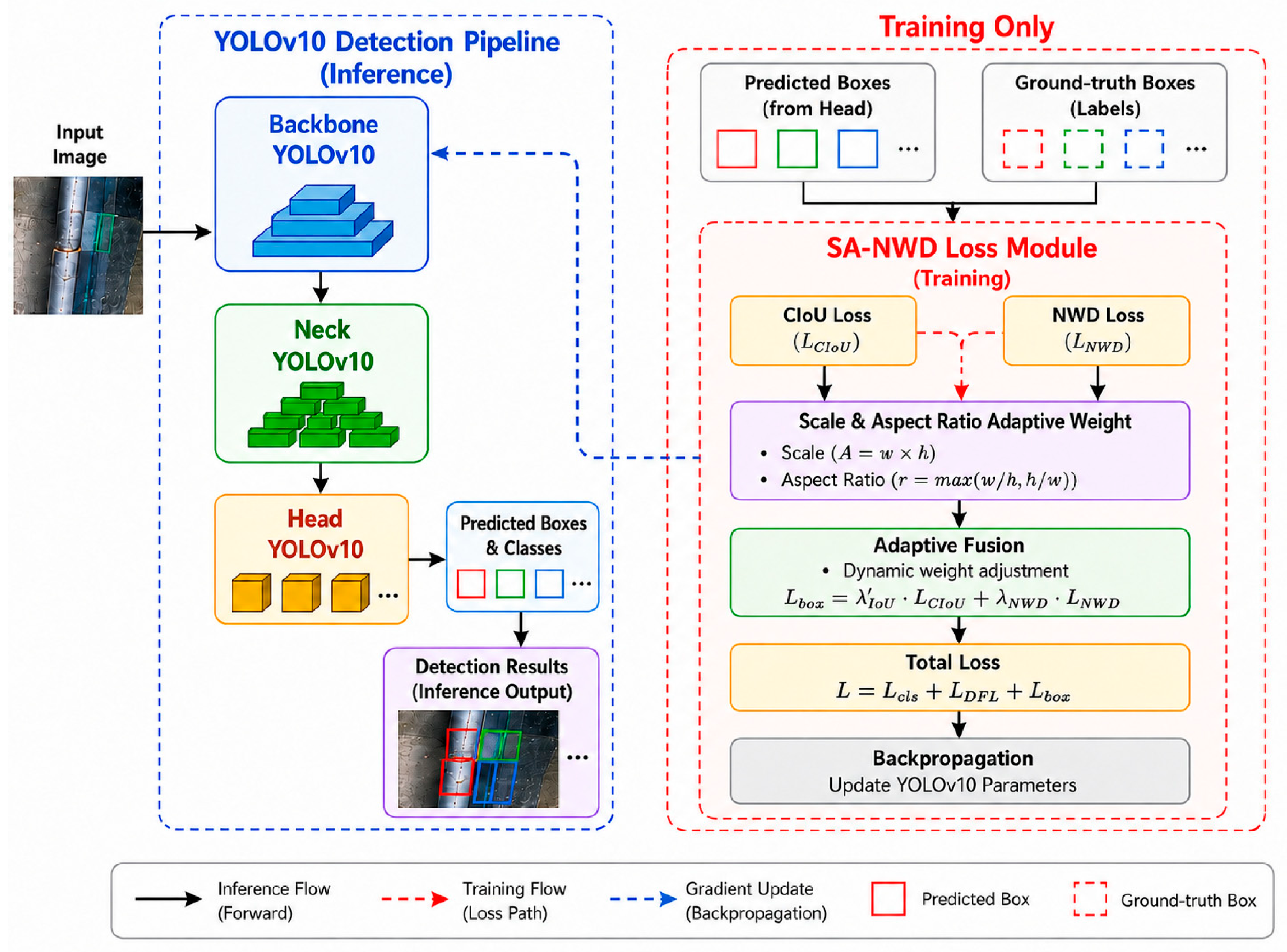
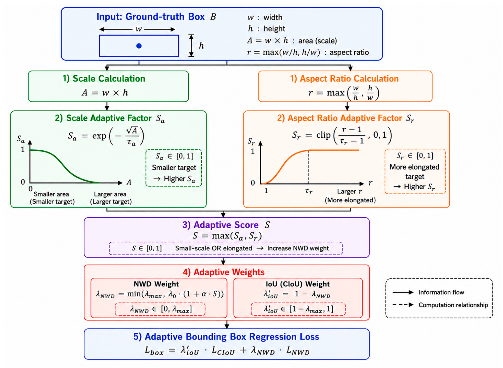
Model-structure-level improvements often increase model complexity, and their performance gains may be limited on small-scale industrial datasets. In contrast, modifying only the bounding-box regression loss can enhance detection performance without increasing the model complexity during the inference stage. Based on this motivation, this paper proposes the SA-NWD based on the YOLOv10 framework. The proposed loss is built upon the Normalized Wasserstein Distance [28], and the resulting YOLOv10-SA-NWD model is developed for external anti-corrosion coating inspection in long-distance pipeline construction scenarios.

The main contributions of this paper are threefold. First, a real construction-site dataset for external anti-corrosion coating-condition inspection is constructed, containing 1388 visible-light images and 1756 annotated bounding boxes across six coating-condition categories. Second, a morphology-aware NWD regression strategy is formulated and compared with fixed-weight NWD (Fixed-NWD). It adaptively adjusts the NWD regression weight according to target area and aspect ratio, strengthening localization guidance for small or elongated targets while leaving the YOLOv10n inference architecture, parameter count, and GFLOPs unchanged. Third, a comprehensive experimental evaluation of SA-NWD is conducted against the CIoU baseline, Fixed-NWD, EIoU, and WIoU under the same architecture. Evaluation includes a duplicate-filtered test set, class-wise AP analysis, six-seed paired statistical assessment, component ablation, and morphology-grouped detection and localization analysis across target scale and aspect-ratio subgroups.

2. Dataset Construction and Task Challenges

To support the development and evaluation of automated inspection methods, an external anti-corrosion condition inspection dataset was constructed from images collected at long-distance pipeline construction sites. The images were acquired from a long-distance natural gas pipeline construction project in eastern China, covering multiple pipeline laying environments and illumination conditions. The raw images used in this work are routine inspection data from the authors’ affiliated company. Due to commercial confidentiality restrictions, the raw image dataset cannot be made publicly available.

The dataset contains a total of 1388 images and 1756 bounding boxes. The images were collected from real construction sites of long-distance natural gas pipelines using commonly available mobile phones. The original image resolutions varied across devices, and all images were resized to 640 × 640 pixels during model training. The shooting distance and view angle were not strictly fixed, reflecting practical on-site inspection conditions. The dataset covers different construction backgrounds, illumination conditions, pipe surface states, and defect appearances. To improve scene diversity, images from repeated views of the same local area were removed during dataset cleaning whenever possible. A subsequent cross-split audit using SHA-256 file-content hashing and 64-bit difference hashing (dHash), with a Hamming-distance threshold of ≤8 used to screen perceptually similar candidate pairs, identified additional duplicate or near-duplicate test images, which were conservatively excluded from the final evaluation. The cross-split screening identified 35 train–validation, 44 train–test, and 7 validation–test candidate pairs. After automated filtering, the remaining test images were also manually cross-checked against the training and validation splits. One author conducted the initial visual review and a second researcher subsequently verified the results; visually identifiable same-scene, same-pipeline-section, same-local-defect-region, and repeated-view relationships were used as the review criteria, and ambiguous cases were jointly re-examined. No additional visually identifiable same-scene overlaps were found. Because complete scene, location, and acquisition-session identifiers were unavailable for the original dataset, strict scene-level independence cannot be formally guaranteed.

The dataset was randomly divided into training, validation, and test sets at the image level with a ratio of 70%:15%:15%. The training set contains 972 images with 1224 bounding boxes, while the validation and original test sets each contain 208 images, with 260 and 272 bounding boxes, respectively. After duplicate filtering, the final evaluation set comprised 168 images and 212 bounding boxes and is hereafter referred to as the duplicate-filtered internal image-level holdout (or duplicate-filtered test set for brevity). Detailed statistics of the dataset are summarized in

Table 1. Class-wise composition of the dataset and the duplicate-filtered test set.

ID	Class	Train Boxes	Val Boxes	Duplicate-Filtered Test	Original Total	Ratio
0	normal coating	98	20	21	139	7.92%
1	uncoated weld joint	108	22	23	154	8.77%
2	coating mechanical damage	350	79	50	510	29.04%
3	heat-shrink sleeve-edge lifting	208	43	35	295	16.80%
4	disbonding	242	51	46	346	19.70%
5	closure patch cracking	218	45	37	312	17.77%
total	-	1224	260	212	1756	100.00%

Note: “Original total” and “Ratio” refer to the original dataset before duplicate filtering. The duplicate-filtered holdout is a subset of the original test split used exclusively for final evaluation; therefore, the train, validation, and duplicate-filtered holdout columns are not additive to the original total.

. The validation set is used exclusively for model selection and hyperparameter tuning during training, whereas all results reported in the main experiments are obtained on the duplicate-filtered test set.

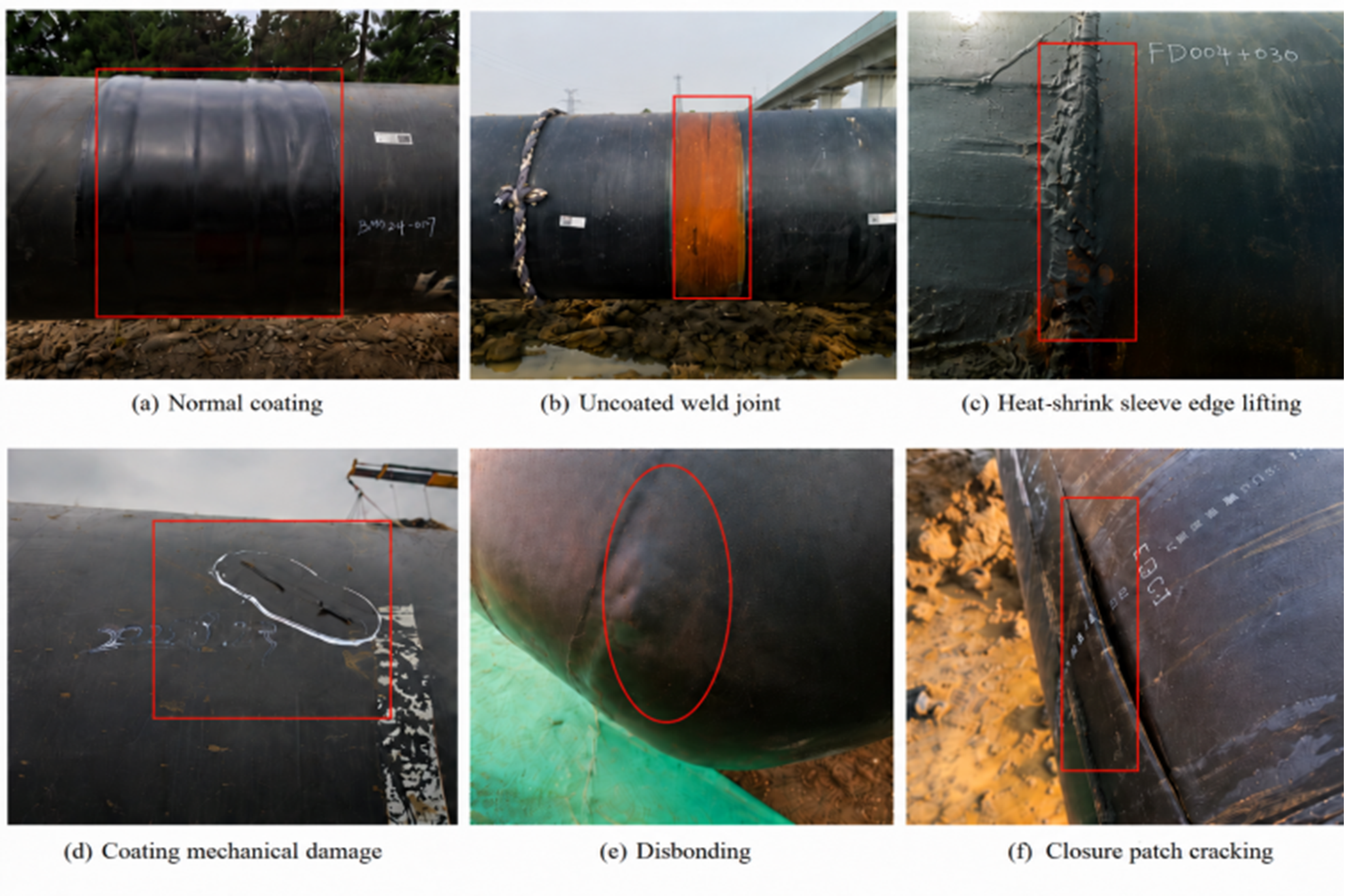
The dataset consists of six categories with fixed class indices: 0—normal coating, 1—uncoated weld joint, 2—coating mechanical damage, 3—heat-shrink sleeve-edge lifting, 4—disbonding, and 5—closure patch cracking. Category 0 represents intact anti-corrosion coating coverage and serves as the non-defect reference. Category 1 indicates incomplete coating application at the weld joint during construction. Categories 2–5 represent typical post-application anti-corrosion coating defects, including mechanical damage, heat-shrink sleeve-edge lifting, disbonding, and closure patch cracking. Representative examples of the six categories are shown in Figure 1.

All images were manually annotated using X-AnyLabeling version 3.0 with bounding-box labels in YOLO format. Two researchers independently performed the annotations, and a domain expert with professional qualifications in pipeline inspection reviewed and adjudicated difficult or disputed samples. Annotation disagreements and ambiguous boundaries were resolved through rule harmonization and standardized annotation procedures to minimize subjective variation. During training, image augmentation strategies, including random scaling, translation, flipping, and color perturbation, were employed to improve the model’s generalization capability under complex on-site imaging conditions [29].

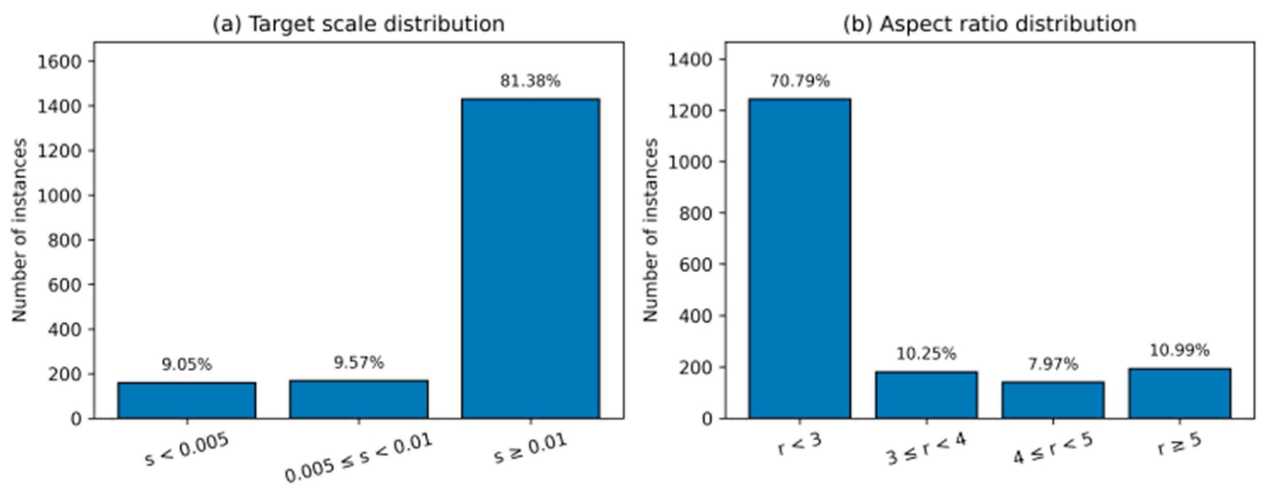
To further analyze the morphological characteristics of the targets in the dataset, the normalized area and aspect ratio distributions of all 1756 annotated bounding boxes were calculated, as shown in Figure 2. The target scale is defined by the normalized area A = w·h, and the aspect ratio is defined as r = max(w/h, h/w). The statistical results show that small-scale targets with a normalized area smaller than 0.01 account for 18.62% of all targets, while those with an area smaller than 0.005 account for 9.05%. In addition, elongated targets (r ≥ 3) account for 29.21%, highly elongated targets (r ≥ 4) account for 18.96%, and extremely elongated targets (r ≥ 5) account for 10.99%.

These results indicate that the dataset contains a certain proportion of small-scale targets and a relatively high proportion of elongated targets. The considerable variations in target scale and aspect ratio make it difficult for conventional bounding-box regression methods to simultaneously satisfy the localization requirements of different target types.

Further analysis of the class distribution and sample morphology shows that coating mechanical damage, disbonding, and closure patch cracking have relatively large numbers of instances, whereas normal coating and uncoated weld joint have relatively fewer instances, indicating an imbalanced class distribution. In terms of morphology, heat-shrink sleeve-edge lifting, closure patch cracking, and some coating mechanical damage targets often exhibit elongated or weak-boundary characteristics, while disbonding targets are mostly planar and characterized by weak texture and low contrast. Overall, the scale distribution, aspect ratio distribution, and inter-class morphological differences demonstrate that external anti-corrosion coating conditions vary significantly in target scale, structural morphology, and boundary clarity. These characteristics collectively motivate the design of the proposed SA-NWD loss.

3. YOLOv10-SA-NWD Method

To address the challenges of large target-scale variations and the prevalence of elongated and weak-boundary targets in external anti-corrosion defect detection, this study proposes an SA-NWD based on the YOLOv10 detection framework. The proposed method improves bounding-box regression by dynamically adjusting the weighting between NWD loss and IoU-based loss according to the scale and aspect ratio of target bounding boxes during training.

3.1. YOLOv10 Baseline Detection Framework

YOLOv10 is a one-stage end-to-end object detection model that adopts a Consistent Dual Assignment (CDA) mechanism to eliminate the need for non-maximum suppression (NMS) post-processing during inference [17]. Its bounding-box regression loss commonly relies on the Complete IoU (CIoU) metric. However, CIoU-based losses are sensitive to localization deviations for small-scale and elongated targets and can suffer from gradient degradation under low-overlap conditions, which limits their localization stability for morphologically complex defects. Therefore, this study improves the bounding-box regression loss. To meet the computational efficiency requirements of real-time industrial inspection, YOLOv10n, the lightest variant of YOLOv10, is selected as the baseline model. The proposed SA-NWD loss introduces several scale- and morphology-related variables and weighting factors. For ease of reference, the principal notations used in the NWD and SA-NWD formulations are summarized in

Table 2. Notations, definitions, and final parameter settings used in NWD and SA-NWD.

Symbol	Description	Final Setting
$W_2^2$	Squared second-order Wasserstein distance	—
C	Normalization constant in NWD	12.8
$L_{NWD}$	Normalized Wasserstein distance loss	—
A	Area of the ground-truth box	—
r	Aspect ratio of the ground-truth box	—
$S_a$	Scale adaptive factor	—
$S_r$	Aspect-ratio adaptive factor	—
S	Final adaptive score	—
${\tau }_a$	Scale adjustment parameter	32
${\tau }_r$	Aspect-ratio adjustment parameter	4.0
α	Adaptive enhancement coefficient	0.30
${\lambda }_{IoU}$	Base weight of the IoU-based loss	0.8
${\lambda }_0$	Base weight of the NWD loss	0.2
${\lambda }_{NWD}$	Adaptive weight of the NWD loss	Equation (8)
${\lambda }_{IoU}^{\prime }$	Complementary weight of the IoU-based loss	Equation (9)
${\lambda }_{max}$	Upper bound of NWD weight	0.3
$L_{CIoU}$	Complete IoU loss	—
$L_{box}$	Bounding-box regression loss	Equation (10)

.

As shown in Figure 3, the proposed method uses YOLOv10n as the baseline detection framework while keeping its original detection architecture unchanged. During training, the model simultaneously calculates the IoU-based bounding-box regression loss and the NWD loss. The NWD constraint weight is then dynamically adjusted according to the scale and aspect ratio of the ground-truth boxes, thereby constructing a scale–aspect adaptive bounding-box regression loss. SA-NWD operates exclusively during the training stage and does not modify the network’s forward inference structure. Consequently, the resulting model retains the parameter count and GFLOPs of the YOLOv10n baseline.

3.2. NWD Bounding-Box Regression Loss

NWD quantifies the geometric discrepancy between a predicted box and a ground-truth box by measuring differences in their center coordinates and dimensions, and converts this discrepancy into a normalized similarity score. Let the predicted box and the ground-truth box be denoted as (x_p, y_p, w_p, h_p) and (x_g, y_g, w_g, h_g), respectively, where (x,y), w, and h represent the box center coordinates, width, and height. For the horizontal bounding boxes used in this study, the squared second-order Wasserstein distance can be simplified as follows [28]:

$$W_2^2={(x_p-x_g)}^2+{(y_p-y_g)}^2+{\left({\displaystyle \frac{w^p-w^g}{2}}\right)}^2+{\left({\displaystyle \frac{h^p-h^g}{2}}\right)}^2$$

(1)

The Normalized Wasserstein Distance (NWD) and the corresponding loss are defined as

$$NWD=exp(-\sqrt{W_2^2}/C)$$

(2)

$$L_{NWD}=1-NWD$$

(3)

where C is the normalization constant of NWD. It should be noted that this study does not use NWD to completely replace the IoU-based loss. Instead, NWD is introduced as an auxiliary constraint and combined with CIoU through weighted fusion to form the bounding-box regression loss. The final value of C, together with the other hyperparameter settings used in the experiments, is summarized in Table 2.

3.3. SA-NWD Loss

The conventional NWD loss applies a fixed loss weight uniformly to all targets, regardless of their scale or aspect ratio, which limits its ability to provide stronger regression constraints for morphologically challenging targets. To address this limitation, this study dynamically adjusts the NWD constraint strength according to the scale and aspect ratio of the target bounding box. Let the width, height, and normalized area of a target box be denoted as w, h, and A = w·h, respectively. The scale factor and aspect ratio factor are defined as

$$S_a=exp(-\sqrt{A}/{\tau }_a)$$

(4)

r = max(w/h, h/w)

(5)

$$S_r=clip({\displaystyle \frac{r-1}{{\tau }_r-1}},\mathrm{0,1})$$

(6)

where ${\tau }_a$ is the scale adjustment parameter and ${\tau }_r$ is the aspect ratio adjustment parameter. A smaller target area leads to a larger $S_a$, whereas a more elongated target shape leads to a larger $S_r$. The final adaptive score is obtained by taking the maximum of these two factors:

$$\mathrm{S} = \max (S_a,S_r)$$

(7)

This design enhances the NWD constraint as long as the target exhibits either a small scale or an elongated morphology. The max operation is adopted rather than simple averaging to ensure that targets exhibiting either characteristic—small scale or high aspect ratio—receive sufficient NWD constraint, preventing the adaptive enhancement from being weakened by averaging with a near-zero factor.

The base NWD weight is defined as ${\lambda }_0=1-{\lambda }_{IoU}$, where ${\lambda }_{IoU}$ denotes the base weight assigned to the IoU-based loss component. The adaptive NWD weight and the corresponding IoU weight are then calculated as

$${\lambda }_{NWD}=\min ({\lambda }_{max},{\lambda }_0·(1+\mathsf{\alpha }\mathrm{S}))$$

(8)

$${\lambda }_{IoU}^{\prime }=1-{\lambda }_{NWD}$$

(9)

where α is the adaptive enhancement coefficient and ${\lambda }_{max}$ is the upper bound of the NWD weight. The parameter ${\lambda }_{max}$ is used to prevent the NWD term from excessively dominating the bounding-box regression loss, thereby avoiding the weakening of the CIoU boundary alignment capability for high-overlap boxes and ensuring stable training. The constraint ${\lambda }_{max}\ge {\lambda }_0$ must be satisfied to ensure that the adaptive mechanism can provide a meaningful weight gain beyond the base NWD weight.

Figure 4 illustrates the adaptive weighting process of SA-NWD. Given a ground-truth box, the scale factor $S_a$ and aspect ratio factor $S_r$ are first computed. Their maximum value is taken as the final adaptive score S, which is then used to derive the dynamic NWD weight ${\lambda }_{NWD}$ and the complementary IoU weight ${\lambda }_{\mathrm{I}\mathrm{o}\mathrm{U}}\prime$. This design ensures that morphologically challenging targets—those that are small-scale, elongated, or both—receive stronger NWD constraints, while regular targets retain the boundary alignment benefit of the IoU-based loss.

3.4. Training Objective of YOLOv10-SA-NWD

The per-target bounding-box regression loss is formulated by combining the CIoU loss and the NWD loss with adaptive weights as follows:

$$L_{box}={\lambda }_{IoU}^{\prime }·L_{CIoU}+ {\lambda }_{NWD}·L_{NWD}$$

(10)

The classification loss ($L_{cls}$) and the Distribution Focal Loss ($L_{DEL}$) are kept unchanged; only the original bounding-box regression loss is replaced with ($L_{box}$) defined in Equation (10). The overall training loss is given by

$$L=L_{cls}+L_{DFL}+L_{box}$$

(11)

Through this design, YOLOv10-SA-NWD provides stronger NWD constraints for small-scale and elongated targets during training, while preserving the IoU boundary alignment capability for regular targets. As noted in Section 3.1, the inference architecture, parameter count, and GFLOPs remain unchanged from those of the YOLOv10n baseline.

4. Experimental Results and Analysis

4.1. Experimental Environment and Parameter Settings

All experiments were conducted on the AutoDL cloud computing platform using a single Tesla V100S-PCIE-32GB GPU for training and testing. The experimental environment consisted of Python 3.12.3, PyTorch 2.3.0+cu121, CUDA 12.1, and Ultralytics 8.4.65 [30]. All models were trained under the same configuration: the input image size was set to (640 × 640), the maximum number of training epochs was 150, the batch size was 16, and the AdamW optimizer was adopted with an initial learning rate of 0.001, momentum of 0.9, and weight decay of 0.0005. All models were initialized from the same pretrained YOLOv10n checkpoint: yolov10n.pt. A linear learning-rate schedule was used (cos_lr = False, lrf = 0.01) with a three-epoch warm-up. The training augmentations were set to hsv_h = 0.015, hsv_s = 0.7, hsv_v = 0.4, translate = 0.1, scale = 0.5, fliplr = 0.5, and mosaic = 1.0, with mosaic augmentation disabled during the final 10 epochs.

To evaluate model stability, repeated experiments were conducted using six random seeds (0, 1, 2, 3, 4, and 42). For each run, the corresponding seed was passed to the Ultralytics training configuration with deterministic training enabled to control the Python, NumPy, PyTorch, and CUDA random-number generators. During training, an Early Stopping strategy with a patience of 50 was applied, and the model weights with the best performance on the validation set, as measured by mAP@0.5:0.95, were used for final evaluation. The validation set was also used exclusively for model selection and hyperparameter tuning, whereas the test set was not used for training, model selection, or hyperparameter optimization. All compared methods used the same dataset split. Following a retrospective cross-split duplicate audit based on exact file-content hashing and perceptual hashing, 32 test images involved in exact cross-split duplicates and eight additional near-duplicate candidates were conservatively excluded. The remaining 168 images containing 212 annotated instances constituted the duplicate-filtered test set used for all final evaluations. Chronologically, dataset partitioning preceded all model development; training was performed on the training subset, model and hyperparameter selection used the validation subset, and the model configurations and checkpoints were fixed before the retrospective duplicate audit and final re-evaluation. Neither the original test split nor the duplicate-filtered holdout was used for architecture design, loss-parameter selection, training-setting adjustment, hyperparameter tuning, checkpoint selection, or image-exclusion decisions, and no model was retrained or further adjusted after duplicate filtering.

4.2. Evaluation Metrics

Precision (P), Recall (R), AP, and mAP were used to evaluate detection performance. Precision and Recall are defined as P = TP/(TP + FP) and R = TP/(TP + FN), respectively, where TP, FP, and FN denote the numbers of true positives, false positives, and false negatives. In industrial defect inspection, missed detections usually carry higher risk than false detections; therefore, Recall is treated as the primary evaluation metric, with mAP used as a complementary measure of overall detection and localization performance.

AP represents the average Precision of a single class over different Recall levels, while mAP denotes the mean AP over all classes. Following established object detection evaluation protocols, mAP@0.5 is adopted from the PASCAL VOC benchmark [31], and mAP@0.5:0.95 is adopted from the MS COCO benchmark [32]. Specifically, mAP@0.5 denotes mAP at an IoU threshold of 0.5, whereas mAP@0.5:0.95 denotes the averaged mAP over IoU thresholds from 0.5 to 0.95 with a step size of 0.05. Accordingly, class-wise performance is reported as AP@0.5, whereas the overall performance averaged across all classes is reported as mAP@0.5 or mAP@0.5:0.95. In addition, the number of parameters (Params) and giga floating-point operations (GFLOPs) were reported to evaluate model complexity. All prediction files used in the morphology-grouped evaluation were generated using the official Ultralytics repository, version 8.4.65 (commit 7a7ad0d). For detection validation, no confidence threshold was explicitly overridden; therefore, the Ultralytics default validation threshold of 0.001 was used. YOLOv10n used its native end-to-end inference without conventional NMS post-processing. The morphology-grouped target-level Recall reported in Section 4.10 is calculated using a separate fixed matching protocol and is therefore distinguished from the standard validator-reported Recall used in the main experiments.

4.3. Main Experiments: Comparison with the Baseline and Fixed-NWD

As NWD and SA-NWD modify only the training-stage bounding-box regression loss, the number of parameters and GFLOPs remain identical to those of the YOLOv10n baseline, as shown in

Table 3. Overall performance comparison of different methods on the test set (mean ± SD over six seeds).

Method	P	R	mAP@0.5	mAP@0.5:0.95	Params	GFLOPs
YOLOv10n	0.522 ± 0.050	0.437 ± 0.020	0.431 ± 0.013	0.240 ± 0.005	2.27M	6.5
Fixed-NWD	0.561 ± 0.063	0.430 ± 0.033	0.442 ± 0.015	0.251 ± 0.011	2.27M	6.5
SA-NWD	0.544 ± 0.081	0.459 ± 0.013	0.451 ± 0.024	0.242 ± 0.013	2.27M	6.5

.

Both Fixed-NWD and SA-NWD show improvements over the YOLOv10n baseline on several evaluation metrics. Compared with the baseline, Fixed-NWD improves the mean mAP@0.5 from 0.431 to 0.442 and the mean mAP@0.5:0.95 from 0.240 to 0.251, indicating that NWD has a more consistent positive effect on localization metrics under higher IoU thresholds. SA-NWD improves the mean Recall from 0.437 to 0.459 and the mean mAP@0.5 from 0.431 to 0.451, achieving the highest mean Recall and mAP@0.5 among the three methods. This suggests that the morphology-adaptive weighting strategy may enhance detection sensitivity, with category-level effects further analyzed in Section 4.6. It should be noted that the mAP@0.5:0.95 of SA-NWD is lower than that of Fixed-NWD, suggesting that its improvement in fine-grained localization under higher IoU thresholds is limited. The uncertainty and statistical evidence associated with these performance differences are further assessed in Section 4.7 using paired analyses across six matched random seeds.

4.4. Comparison with Representative Bounding-Box Regression Losses

To assess whether the performance of SA-NWD is competitive relative to other representative bounding-box regression losses, comparative experiments were conducted across the same six random seeds used in the main experiments (0, 1, 2, 3, 4, and 42). The compared methods include EIoU, which explicitly decouples aspect-ratio differences in regression, and WIoU, which introduces a dynamic focusing mechanism based on sample quality. Results are summarized in

Table 4. Comparison with representative bounding-box regression losses (mean ± SD over six seeds).

Method	P	R	mAP@0.5	mAP@0.5:0.95
YOLOv10n (CIoU)	0.522 ± 0.050	0.437 ± 0.020	0.431 ± 0.013	0.240 ± 0.005
EIoU	0.446 ± 0.062	0.377 ± 0.030	0.363 ± 0.020	0.205 ± 0.012
WIoU	0.566 ± 0.045	0.450 ± 0.012	0.448 ± 0.014	0.245 ± 0.008
Fixed-NWD	0.561 ± 0.063	0.430 ± 0.033	0.442 ± 0.015	0.251 ± 0.011
SA-NWD	0.544 ± 0.081	0.459 ± 0.013	0.451 ± 0.024	0.242 ± 0.013

.

SA-NWD achieves the highest mean Recall (0.459) and mAP@0.5 (0.451), whereas Fixed-NWD achieves the highest mean mAP@0.5:0.95 (0.251), and WIoU achieves the highest mean Precision (0.566) among all compared methods across the six-seed evaluation. WIoU also improves mean mAP@0.5 from 0.431 to 0.448 relative to the CIoU baseline, whereas EIoU shows lower mean performance across all four evaluation metrics. WIoU remains competitive in this dataset, particularly in Precision and mAP@0.5, indicating that its dynamic focusing mechanism can also provide benefits for the present inspection task. These results suggest that general-purpose regression losses designed for large-scale benchmarks do not transfer uniformly to domain-specific defect datasets, while the two NWD-based strategies exhibit different performance tendencies: SA-NWD favors Recall and mAP@0.5, whereas Fixed-NWD favors mAP@0.5:0.95. The mean ± SD results over six matched random seeds reduce the dependence of this comparison on a particular initialization, although the differences among methods should still be interpreted together with the uncertainty analysis in Section 4.7.

4.5. Ablation Study of SA-NWD Components

To validate the contribution of the scale factor and aspect-ratio factor in SA-NWD, two ablation variants were evaluated across the same six random seeds used in the main experiments: Scale-only NWD, which applies adaptive NWD weighting based solely on target area, and Aspect-only NWD, which applies adaptive weighting based solely on aspect ratio. Results are summarized in

Table 5. Ablation study of the morphology-adaptive components (mean ± SD over six seeds).

Method	P	R	mAP@0.5	mAP@0.5:0.95
CIoU baseline	0.522 ± 0.050	0.437 ± 0.020	0.431 ± 0.013	0.240 ± 0.005
Fixed-NWD	0.561 ± 0.063	0.430 ± 0.033	0.442 ± 0.015	0.251 ± 0.011
Scale-only NWD	0.504 ± 0.053	0.435 ± 0.026	0.426 ± 0.020	0.235 ± 0.012
Aspect-only NWD	0.526 ± 0.056	0.440 ± 0.011	0.433 ± 0.024	0.239 ± 0.016
SA-NWD (full)	0.544 ± 0.081	0.459 ± 0.013	0.451 ± 0.024	0.242 ± 0.013

.

The full SA-NWD achieves higher mean Recall and mAP@0.5 than both single-factor variants, indicating that the combined formulation performs more favorably than using either adaptive factor alone. Scale-only NWD achieves a mean Recall of 0.435, close to the baseline value of 0.437, while its mAP@0.5 and mAP@0.5:0.95 are slightly lower than those of the baseline. Aspect-only NWD shows similarly modest changes relative to the baseline, with mean Recall increasing from 0.437 to 0.440 and mAP@0.5 from 0.431 to 0.433, while mAP@0.5:0.95 remains comparable (0.239 vs. 0.240). The full SA-NWD combines both factors and achieves the best mean Recall (0.459) and mAP@0.5 (0.451) among the baseline and adaptive variants, with mAP@0.5:0.95 (0.242) also exceeding both Scale-only NWD (0.235) and Aspect-only NWD (0.239). These results suggest that combining scale- and aspect-ratio-dependent weighting is more effective than either single-factor formulation for improving mean Recall and mAP@0.5, although the individual factors alone do not provide consistent improvements over the baseline across all metrics.

4.6. Class-Wise Performance and Confusion Matrix Analysis

Table 6. Class-wise AP@0.5 on the test set (mean ± SD over six seeds).

Category	n	YOLOv10n	Fixed-NWD	SA-NWD	ΔSA-NWD—Baseline	ΔSA-NWD—Fixed-NWD
normal coating	21	0.708 ± 0.034	0.737 ± 0.031	0.729 ± 0.018	+0.022	−0.008
uncoated weld joint	23	0.832 ± 0.058	0.870 ± 0.033	0.843 ± 0.062	+0.011	−0.028
coating mechanical damage	50	0.536 ± 0.050	0.530 ± 0.026	0.566 ± 0.033	+0.030	+0.037
heat-shrink sleeve-edge lifting	35	0.100 ± 0.017	0.071 ± 0.019	0.106 ± 0.041	+0.006	+0.035
disbonding	46	0.159 ± 0.021	0.171 ± 0.035	0.171 ± 0.029	+0.012	0.000
closure patch cracking	37	0.250 ± 0.061	0.272 ± 0.087	0.293 ± 0.057	+0.042	+0.021

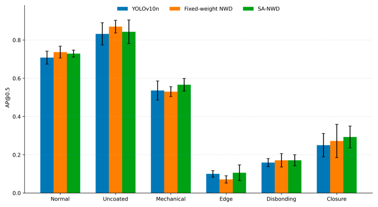
Note: Δ values were calculated from unrounded seed-wise means; apparent differences of 0.001 from the displayed means reflect rounding. Bold values indicate the highest mean AP@0.5 within each category.

and Figure 5 present the class-wise AP@0.5 results and their visual comparison, respectively, showing that the three loss functions exhibit distinct effects across different inspection categories. Compared with the baseline, SA-NWD improves AP@0.5 by 0.030 for coating mechanical damage and by 0.042 for closure patch cracking. Both SA-NWD and Fixed-NWD achieve modest gains of approximately 0.012 for disbonding, indicating that NWD-based losses provide similar positive mean changes for weak-boundary planar targets. Fixed-NWD achieves larger gains than SA-NWD for normal coating and uncoated weld joint, whereas SA-NWD achieves larger gains for closure patch cracking. For heat-shrink sleeve-edge lifting, Fixed-NWD decreases AP@0.5 by 0.029, whereas SA-NWD remains nearly unchanged (+0.006), suggesting that the adaptive weighting mechanism may mitigate the negative effect of fixed weighting on this category.

Overall, SA-NWD shows relatively better detection performance for coating mechanical damage and closure patch cracking, whereas Fixed-NWD achieves higher mean AP@0.5 for normal coating and uncoated weld joint. These results suggest that SA-NWD shows more favorable mean performance for several morphologically variable defect categories, although neither NWD-based strategy provides uniform improvement across all categories.

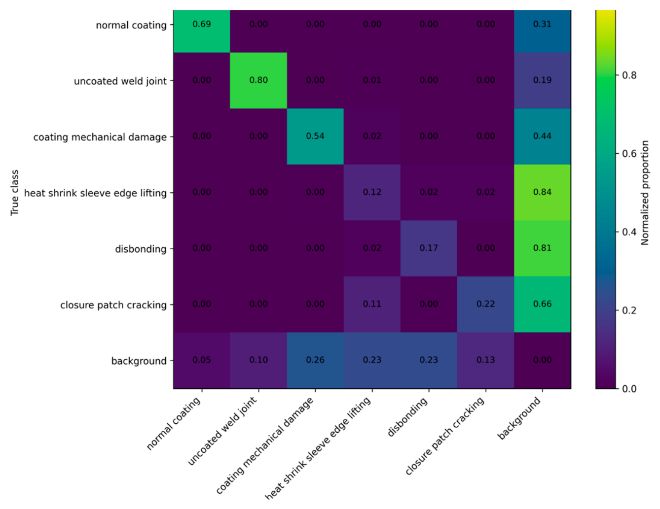
To further analyze class confusion, Figure 6 presents the aggregated normalized confusion matrix of SA-NWD on the test set across six random seeds. The confusion matrix provides a complementary view of the remaining classification errors and background-related false detections. The dominant error mode for heat-shrink sleeve-edge lifting is missed detection rather than inter-class confusion, with 0.838 of the aggregated ground-truth instances assigned to background. Disbonding and closure patch cracking also show relatively high background proportions of 0.812 and 0.662, respectively, whereas direct confusion among defect classes is generally limited. Among unmatched background-related false-positive predictions, coating mechanical damage, disbonding, and heat-shrink sleeve-edge lifting account for the largest proportions (0.262, 0.233, and 0.230, respectively), suggesting that complex background textures may resemble the local visual characteristics of these defect categories. Because the class-wise sample sizes are limited, the observed category-specific differences are interpreted descriptively rather than as statistically established effects.

It is worth noting that the AP@0.5 of heat-shrink sleeve-edge lifting is lower than 0.11 under all three methods, making it the most challenging category in the current dataset. This may be attributed to its elongated morphology, blurred boundaries, background interference, and relatively limited sample size. This category therefore warrants further investigation, as discussed in Section 5.

4.7. Multi-Seed Stability and Exploratory Statistical Analysis

To assess the uncertainty of performance differences between methods, paired analyses were conducted across six matched experiments with different random seeds. Recall for SA-NWD versus the YOLOv10n baseline was treated as the primary comparison, while the remaining comparisons were considered secondary exploratory analyses. Paired mean differences, 95% confidence intervals, Cohen’s ($d_z$), and exact two-sided sign-flip permutation tests were calculated, with the 95% confidence intervals calculated from the six paired seed-wise differences using two-sided t-based intervals. Holm correction was applied to the secondary comparisons, defined as the remaining eight method–metric comparisons in

Table 7. Exploratory paired statistical comparisons across six matched random seeds.

Comparison	Metric	Mean Difference (A–B)	95% CI	Cohen’s ${\mathit{d}}_{\mathit{z}}$	Exact Permutation p	Holm-Adjusted p
SA–NWD vs. Baseline	Recall	+0.0223	[−0.0048, 0.0494]	0.865	0.0938	—
SA–NWD vs. Baseline	mAP@0.5	+0.0205	[−0.0013, 0.0423]	0.987	0.0938	0.7500
SA–NWD vs. Baseline	mAP@0.5:0.95	+0.0025	[−0.0072, 0.0122]	0.271	0.5938	1.0000
Fixed-NWD vs. Baseline	Recall	−0.0062	[−0.0351, 0.0228]	−0.224	0.5625	1.0000
Fixed-NWD vs. Baseline	mAP@0.5	+0.0110	[−0.0111, 0.0331]	0.522	0.2500	1.0000
Fixed-NWD vs. Baseline	mAP@0.5:0.95	+0.0117	[−0.0002, 0.0235]	1.035	0.0938	0.7500
SA–NWD vs. Fixed-NWD	Recall	+0.0285	[−0.0025, 0.0595]	0.965	0.0938	0.7500
SA–NWD vs. Fixed-NWD	mAP@0.5	+0.0095	[−0.0217, 0.0407]	0.319	0.5000	1.0000
SA–NWD vs. Fixed-NWD	mAP@0.5:0.95	–0.0092	[−0.0297, 0.0113]	−0.469	0.3125	1.0000

after excluding the prespecified primary comparison of SA-NWD versus the baseline in Recall. Paired t-tests and Wilcoxon signed-rank tests were additionally used as sensitivity analyses. The six matched seeds quantify variability associated with stochastic model optimization and initialization rather than sampling uncertainty across independent scenes, projects, or deployment sites. The statistical results are shown in Table 7. Compared with the YOLOv10n baseline, SA-NWD achieves a mean Recall increase of 0.0223 (95% CI: −0.0048 to 0.0494; ($d_z$ = 0.865)), although the exact permutation test did not reach the conventional significance level (p = 0.0938). SA-NWD also achieves a mean mAP@0.5 increase of 0.0205 ($d_z$ = 0.987), but its confidence interval includes zero and the Holm-adjusted permutation (p)-value is 0.7500. Fixed-NWD increases mean mAP@0.5:0.95 by 0.0117 ($d_z$ = 1.035), but this difference is likewise not statistically established (95% CI: −0.0002 to 0.0235; exact permutation (p = 0.0938)). In addition, SA-NWD shows a higher mean Recall than Fixed-NWD (+0.0285), with a relatively large paired effect size ($d_z$ = 0.965), although the corresponding confidence interval also includes zero.

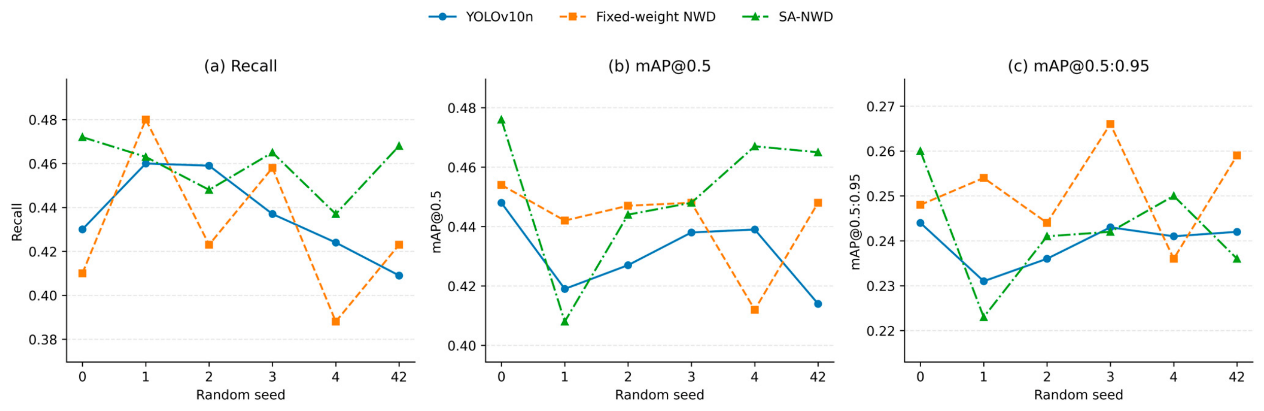
Figure 7 illustrates the performance trends of YOLOv10n, Fixed-NWD, and SA-NWD across six random seeds. The curves for all three methods remain relatively stable across different seeds, indicating consistent training behavior. Although SA-NWD shows higher mean Recall and mAP@0.5, while Fixed-NWD shows higher mean mAP@0.5:0.95, the performance ranges of the three methods overlap across seeds, consistent with the uncertainty reflected in Table 7.

Overall, the multi-seed experiments indicate that both NWD-based losses yield consistent performance across different random initializations. SA-NWD shows favorable mean trends in Recall and mAP@0.5, whereas Fixed-NWD shows a favorable mean trend in mAP@0.5:0.95. However, none of these differences are statistically established under the current six-seed paired analysis. Therefore, the observed differences should be interpreted as performance trends with corresponding effect sizes and uncertainty rather than evidence of statistical superiority, and further validation on larger and more diverse datasets is warranted. The complete per-seed results and paired statistical analyses are provided in Supplementary Tables S1 and S2, respectively.

4.8. Hyperparameter Selection and Sensitivity Analysis

This section analyzes the sensitivity of model performance to two sets of hyperparameters: the NWD normalization constant C and the SA-NWD-specific parameters α and ${\lambda }_{max}$. All hyperparameter exploration was conducted exclusively on the validation set during model development, and the test set was not used for parameter selection. The final parameter settings adopted in the main experiments are summarized in Table 2, while the corresponding validation-set sensitivity results are reported in

Table 8. Hyperparameter sensitivity analysis on the validation set during model development.

Parameter	Setting	P	R	mAP@0.5	mAP@0.5:0.95
C	8.0	0.5979	0.4975	0.4642	0.2398
C	12.8	0.5897	0.4635	0.4644	0.2603
C	16.0	0.6249	0.5066	0.5018	0.2580
$\alpha , {\lambda }_{max}$	1.0, 0.45	0.557 ± 0.038	0.525 ± 0.018	0.477 ± 0.018	0.249 ± 0.014
$\alpha , {\lambda }_{max}$	0.3, 0.30	0.583 ± 0.052	0.513 ± 0.016	0.478 ± 0.027	0.255 ± 0.012

.

To analyze the effect of C on model performance, comparative experiments were conducted with C = 8.0, 12.8, and 16.0 while keeping the other parameters unchanged. As shown in Table 8, increasing C from 12.8 to 16.0 raises validation mAP@0.5 from 0.4644 to 0.5018, whereas mAP@0.5:0.95 reaches its highest value at C = 12.8 (0.2603) and slightly decreases to 0.2580 at C = 16.0. These results indicate that C affects the balance between moderate-IoU detection performance and localization performance at stricter IoU thresholds, rather than producing a uniformly optimal value across all metrics. Accordingly, C = 12.8 was retained because it achieved the highest validation mAP@0.5:0.95 while maintaining competitive mAP@0.5 performance. It should be noted that the experiment with C = 8.0 terminated early at epoch 139 due to the Early Stopping criterion, whereas the C = 12.8 and C = 16.0 configurations completed 150 epochs. The C = 8.0 result should therefore be interpreted with additional caution.

In addition to the normalization constant C, the adaptive enhancement coefficient α and the upper bound of the NWD weight ${\lambda }_{max}$ in SA-NWD also affect the relative contribution of NWD and CIoU in the bounding-box regression loss. Their validation-set results are also summarized in Table 8. When the more aggressive configuration, α = 1.0 and ${\lambda }_{max}$ = 0.45, is used, Recall increases to 0.525, but Precision and mAP@0.5:0.95 decrease to 0.557 and 0.249, respectively. In contrast, when the milder configuration, α = 0.3 and ${\lambda }_{max}$ = 0.30, is used, Precision increases to 0.583 and mAP@0.5:0.95 to 0.255, while mAP@0.5 remains essentially unchanged (0.478 vs. 0.477). This indicates that excessively aggressive adaptive weighting can favor Recall at the expense of localization quality, consistent with the role of ${\lambda }_{max}$ described in Section 3.3. Therefore, α = 0.3 and ${\lambda }_{max}$ = 0.30 are adopted as the default hyperparameter configuration for SA-NWD, as this setting provides a more balanced validation performance across detection sensitivity and high-IoU localization. No further hyperparameter adjustment was performed using the test set.

4.9. Visualization Analysis

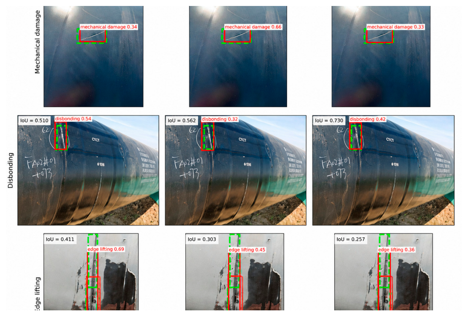
In the representative examples shown in Figure 8, SA-NWD produces predicted bounding boxes with tighter and more accurate fits to the target regions. These visual results provide qualitative support for the quantitative performance trends observed in Table 3 and the category-level differences reported in Table 6, particularly for morphologically complex coating conditions. However, these examples are intended as qualitative illustrations rather than evidence of consistent superiority across all samples.

For heat-shrink sleeve-edge lifting samples, all three methods exhibit missed detections or localization deviations, with no consistent advantage observed among them. This observation is consistent with the class-wise AP results in Table 6, where heat-shrink sleeve-edge lifting shows AP@0.5 below 0.11 across all three methods.

4.10. Morphology-Grouped Detection and Localization Analysis

To assess whether the morphology-adaptive weighting of SA-NWD translates into differential detection performance across target subgroups, target-level Recall and matched IoU were computed separately for targets grouped by normalized area and aspect ratio using bounding-box predictions from all 18 runs (three methods × six seeds). Similar scale-aware evaluation strategies have been adopted in previous studies to analyze detector sensitivity to small targets [33]. Predictions retained at the validation confidence threshold of 0.001 were sorted in descending order of confidence and greedily matched one-to-one to unmatched ground-truth targets of the same class. For each prediction, the unmatched same-class ground-truth target with the highest IoU was selected, and the match was accepted when IoU ≥ 0.5. Once a ground-truth target was matched, subsequent duplicate predictions could not generate additional true positives. The resulting target-level Recall differs from the standard validator-reported Recall in Table 3, while matched IoU represents the mean IoU of the corresponding matched detections. Target-level Recall was calculated as the number of matched targets divided by the total number of targets in each morphology group, and both target-level Recall and matched IoU were first calculated independently for each run and then summarized as the arithmetic mean ± population standard deviation (ddof = 0) across the six seeds. The standard Ultralytics Recall in Table 3 is reported at the confidence operating point corresponding to the maximum smoothed mean F1 score, whereas the morphology-grouped Recall uses the predictions retained at confidence ≥ 0.001; the two Recall values therefore have different operating-point definitions and are not expected to be numerically identical. Groups were defined as small (A < 0.01, n = 45), regular size (A ≥ 0.01, n = 167), moderate elongated (3 ≤ r < 5, n = 50), extreme elongated (r ≥ 5, n = 21), regular shape (r < 3, n = 141), and hard targets (small or elongated, n = 111). Results are summarized in

Table 9. Exploratory morphology-grouped target-level detection and localization analysis (mean ± SD over six seeds).

Morphology Group	n	Target-Level Recall (IoU ≥ 0.5)			Matched IoU (Matched Detections)
		Baseline	Fixed-NWD	SA-NWD	Baseline	Fixed-NWD	SA-NWD
All	212	0.647 ± 0.034	0.637 ± 0.033	0.649 ± 0.025	0.709 ± 0.008	0.718 ± 0.003	0.713 ± 0.008
Small (A < 0.01)	45	0.678 ± 0.046	0.696 ± 0.036	0.696 ± 0.025	0.669 ± 0.015	0.683 ± 0.011	0.671 ± 0.013
Regular size (A ≥ 0.01)	167	0.639 ± 0.036	0.621 ± 0.037	0.636 ± 0.027	0.721 ± 0.007	0.729 ± 0.007	0.725 ± 0.008
Moderately elongated (3 ≤ r < 5)	50	0.573 ± 0.038	0.547 ± 0.044	0.573 ± 0.062	0.674 ± 0.015	0.672 ± 0.015	0.679 ± 0.019
Extremely elongated (r ≥ 5)	21	0.706 ± 0.033	0.659 ± 0.101	0.714 ± 0.027	0.678 ± 0.012	0.693 ± 0.030	0.685 ± 0.022
Regular shape (r < 3)	141	0.664 ± 0.040	0.665 ± 0.030	0.665 ± 0.028	0.725 ± 0.013	0.736 ± 0.004	0.728 ± 0.007
Hard *	111	0.637 ± 0.034	0.631 ± 0.041	0.646 ± 0.034	0.674 ± 0.009	0.682 ± 0.008	0.679 ± 0.012

Note: Target-level Recall was calculated using a fixed evaluation protocol with predictions retained at confidence ≥ 0.001 and greedy one-to-one correct-class matching at IoU ≥ 0.5. Once a ground-truth target was matched, subsequent duplicate predictions could not generate additional true positives. This metric differs from the standard validator-reported Recall in Table 3. Matched IoU denotes the mean IoU of the corresponding matched detections. Morphology groups defined by scale and aspect ratio are not mutually exclusive. * Hard targets are defined as targets that are either small (A < 0.01) or elongated (r ≥ 3).

.

As shown in Table 9, SA-NWD achieves the highest mean target-level recall for the overall set (0.649 ± 0.025), extremely elongated targets (0.714 ± 0.027), and hard targets (0.646 ± 0.034). For extremely elongated targets (r ≥ 5), the mean Recall of SA-NWD is 0.714 ± 0.027 compared with 0.659 ± 0.101 for Fixed-NWD (+5.5 percentage points) and 0.706 ± 0.033 for the baseline (+0.8 percentage points). SA-NWD also exhibits lower cross-seed variability than Fixed-NWD for this subgroup, although the difference relative to the baseline is small. For small targets (A < 0.01), SA-NWD and Fixed-NWD achieve the same mean recall (0.696), both exceeding the baseline (0.678). For moderately elongated targets (3 ≤ r < 5), no consistent advantage is observed across methods, while SA-NWD and the baseline achieve the same mean recall of 0.573. For regular-shape targets, all three methods perform comparably, consistent with the design intent of preserving CIoU boundary alignment for non-challenging targets.

The matched-IoU results show a different pattern. Fixed-NWD achieves the highest mean matched IoU for the overall set and for most morphology groups, including small, regular-size, extremely elongated, regular-shape, and hard targets. Across all 212 targets, the mean matched IoU is 0.718 ± 0.003 for Fixed-NWD, compared with 0.709 ± 0.008 for the baseline and 0.713 ± 0.008 for SA-NWD. This pattern is consistent with the overall results in Table 3, where SA-NWD shows higher mean Recall and mAP@0.5, whereas Fixed-NWD achieves higher mean mAP@0.5:0.95.

It should be noted that the extremely elongated subgroup contains only 21 instances in the test set. The reported morphology-grouped differences should therefore be interpreted as exploratory rather than conclusive. Moreover, the scale- and aspect-ratio-based groups are partially overlapping, and differences in class composition may also contribute to the observed subgroup patterns. Validation on larger datasets with more balanced morphology distributions will be necessary to confirm these findings. The class-wise composition of the morphology subgroups is provided in Supplementary Table S3.

5. Discussion

5.1. Effect of SA-NWD on Recall

As reported in Table 3, SA-NWD achieves the highest mean Recall among the three methods, suggesting that the scale- and aspect-ratio-based adaptive weighting mechanism may have a positive effect on defect detection sensitivity. This improvement is likely because NWD provides continuous geometric distance constraints even under low-overlap conditions, thereby alleviating regression instability for small-scale, elongated, or weak-boundary targets during early training. Compared with Fixed-NWD, SA-NWD dynamically strengthens the NWD constraint for small-scale and elongated targets, which may contribute to the observed increase in overall detection sensitivity. However, the paired mean Recall difference between SA-NWD and the baseline was +0.0223, with a 95% confidence interval crossing zero and an exact permutation (p)-value of 0.0938. Therefore, this result should be interpreted as an average performance trend rather than a statistically established superiority.

5.2. Morphology-Grouped Interpretation of SA-NWD

The morphology-grouped analysis in Section 4.10 provides additional descriptive context for interpreting the morphology-adaptive design of SA-NWD. For extremely elongated targets (r ≥ 5), SA-NWD achieves the highest mean target-level Recall of 0.714, compared with 0.706 for the baseline and 0.659 for Fixed-NWD. For these targets, standard CIoU loss treats boundary misalignments uniformly regardless of elongation direction, whereas SA-NWD amplifies the NWD constraint for high-aspect-ratio boxes, providing stronger centroid-displacement guidance along the elongated axis. The lower cross-seed variability for this subgroup (±0.027 vs. ±0.101 for Fixed-NWD) is also consistent with more stable performance for geometrically irregular targets.

The ablation results in Section 4.5 show that Scale-only NWD and Aspect-only NWD do not consistently improve upon the baseline when used individually. The full SA-NWD combining both factors achieves the best Recall and mAP@0.5, with mAP@0.5:0.95 marginally exceeding Aspect-only NWD. This pattern suggests that scale and aspect-ratio adaptation provide complementary regression guidance that neither single factor alone can fully replicate.

For moderately elongated targets (3 ≤ r < 5), no consistent advantage of SA-NWD over the baseline is observed, indicating that the aspect-ratio-dependent weighting has a more selective effect at higher elongation levels. This finding suggests that the benefit of morphology-adaptive NWD weighting may be more apparent for highly elongated targets. However, the morphology groups partially overlap and may differ in class composition; therefore, class–morphology confounding cannot be completely excluded, and the subgroup results should be interpreted as supportive rather than definitive evidence.

5.3. Difference Between mAP@0.5 and mAP@0.5:0.95

The divergence between mAP@0.5 and mAP@0.5:0.95 reveals a performance trade-off between the two NWD-based losses. SA-NWD achieves the highest average mAP@0.5, indicating a tendency toward improved detection sensitivity, whereas Fixed-NWD achieves a higher mAP@0.5:0.95, suggesting more stable fine-grained localization under higher IoU thresholds. This phenomenon indicates that strengthening the NWD constraint adaptively according to target scale and aspect ratio can improve the detection of difficult targets, but it may not always enhance high-IoU localization accuracy. In contrast, Fixed-NWD provides a more uniform regression constraint for all targets, which may be more favorable for maintaining fine-grained localization consistency across categories. This complementary pattern between SA-NWD and Fixed-NWD is further supported by the morphology-grouped analysis in Section 4.10, where SA-NWD achieves higher target-level Recall for several difficult morphology groups, whereas Fixed-NWD achieves the highest matched IoU for most groups. Together, these results suggest that SA-NWD favors detection sensitivity, while Fixed-NWD tends to provide more consistent high-IoU localization. However, the paired six-seed analyses in Section 4.7 indicate that these differences should be interpreted as performance tendencies rather than statistically established superiority.

5.4. Class Differences and Dataset Limitations

The category-level divergence suggests that morphology-adaptive weighting appears to provide greater benefits for defects with variable shapes and indistinct boundaries, such as coating mechanical damage and closure patch cracking. For categories with more regular morphology, clearer boundary features, or limited training samples, the adaptive mechanism does not consistently outperform fixed weighting. This suggests that the benefit of morphology-adaptive weighting depends on the degree of morphological variability within each category, rather than providing uniform improvement across all defect types.

Despite the overall dataset size of 1388 images and 1756 bounding boxes, the number of samples and the clarity of visual boundaries still vary considerably across categories. These factors may partly explain why the performance gains of SA-NWD are not consistent across all defect types, especially for heat-shrink sleeve-edge lifting, which remains the most difficult category in the current dataset. The aggregated confusion matrix further shows that its dominant error mode is missed detection rather than inter-class confusion. Background-related false-positive predictions are also concentrated mainly in coating mechanical damage, heat-shrink sleeve-edge lifting, and disbonding, indicating that complex construction backgrounds remain an important source of detection difficulty.

The comparison with representative regression losses in Section 4.4 shows that WIoU remains competitive, achieving the highest mean Precision and a mean mAP@0.5 close to that of SA-NWD, whereas EIoU performs less favorably on the present dataset. These results indicate that the relative effectiveness of different regression losses is task-dependent rather than supporting uniform superiority of NWD-based methods.

5.5. Industrial Application Significance

In pipeline anti-corrosion defect inspection, undetected defects may remain unrepaired before pipeline burial and can subsequently lead to local coating failure, pipe body corrosion, and safety risks [1,2,3]. Therefore, the observed improvement trend in Recall has practical engineering relevance, even though it does not reach statistical significance under the current six-seed analysis. Meanwhile, SA-NWD acts only during the training stage and does not change the inference network structure or increase the number of parameters and GFLOPs, thereby preserving the inference complexity of the YOLOv10n baseline. However, latency, memory usage, and edge/mobile-device performance were not measured in the present study; practical field-deployment suitability therefore remains to be validated on target hardware. Nevertheless, the current results are mainly obtained from a visible-light image dataset collected from a limited engineering scenario, and the generalization capability of the proposed approach across diverse construction sites, imaging conditions, and additional difficult-to-detect defect categories warrants further investigation.

6. Conclusions

This study developed a field-acquired dataset for external anti-corrosion coating inspection, comprising 1388 images and 1756 annotated instances across six coating-condition categories collected from long-distance natural gas pipeline construction sites. Building on YOLOv10n, a Scale–Aspect Adaptive Normalized Wasserstein Distance Loss (SA-NWD) is proposed, which dynamically adjusts the NWD regression weight according to the target scale and aspect ratio during training while leaving the YOLOv10n inference architecture, parameter count, and GFLOPs unchanged.

Experiments with six random seeds show that SA-NWD achieves the highest mean Recall (0.459) and mAP@0.5 (0.451) among the three main methods, while Fixed-NWD yields the highest mean mAP@0.5:0.95 (0.251). Paired six-seed analyses indicate that these improvements represent consistent performance trends rather than statistically established superiority. Comparison with EIoU and WIoU under the same six-seed configuration shows that WIoU remains competitive, whereas EIoU performs less favorably on the present dataset. Ablation experiments further support that scale and aspect-ratio adaptation provide complementary regression guidance, with the full SA-NWD outperforming both single-factor variants in Recall and mAP@0.5.

Morphology-grouped analysis shows that SA-NWD achieves the highest mean target-level Recall for extremely elongated targets (r ≥ 5), reaching 0.714 compared with 0.706 for the baseline and 0.659 for Fixed-NWD, while exhibiting lower cross-seed variability than Fixed-NWD (±0.027 vs. ±0.101). For small targets (A < 0.01), both NWD-based strategies outperform the baseline with comparable Recall. These complementary characteristics suggest that SA-NWD shows favorable mean performance for high-recall screening of morphologically complex coating-condition targets, whereas Fixed-NWD provides more stable high-IoU localization.

Several limitations should be noted. The extremely elongated subgroup contains only 21 test instances, and the reported Recall pattern should be interpreted as supportive rather than definitive evidence, particularly because morphology groups may overlap and differ in class composition. The dataset originates from a single construction project, and generalization across diverse sites, imaging conditions, and additional defect categories warrants further investigation. Heat-shrink sleeve-edge lifting and complex-background interference also remain important detection challenges. Future work will explore more systematic scene-level provenance tracking and partitioning, larger multi-site validation, and extension to other morphologically challenging industrial inspection scenarios.