Multiple Imputation of Missing Traffic Volume: An Advanced Framework and Multi-Domain Validation

Abstract

High-frequency traffic data from remote sensors often suffer from severe gaps and multi-day blackouts. Traditional deterministic imputation fails during these extended failures, artificially destroying natural traffic variance. To resolve this, this study develops an adaptive Multiple Imputation (MI) framework to reconstruct missing 2-min volumes. A novel multi-tier historical median predictor with adaptive expansion (up to ±30 min) serves as a variance-protected anchor for two stochastic engines: Stochastic Linear Regression and Predictive Mean Matching with Approximate Bayesian Bootstrap (PMM-ABB). PMM-ABB features dynamic $K$-neighbor autotuning, with simulation convergence governed by a dual-metric algorithm. Performance was evaluated against a Historical Average (HA) baseline via multi-domain validation, strictly assessing the models’ ability to recover hidden, real-world ground-truth counts rather than replicating the engineered input features. Under severe block-missingness, the stochastic models prevented collapse, reducing Temporal Cross-Validation MAE from 33.7 (HA) to 22.7 (Cohen’s $d$ = −0.4). Power Spectral Density matching confirmed that both models preserved macro-periodic traffic waves, keeping spectral tracking errors under 4.8 dB. Ultimately, PMM-ABB slightly outperformed Stochastic Regression in sequential time dependency and point accuracy, confirming that the framework provides a highly reliable structural proxy for continuous highway flow modeling.

1. Introduction

The integrity and completeness of time-series traffic data are the foundational pillars of intelligent transportation systems (ITSs). Raw data collected from the field is usually imperfect [1]. Dynamic traffic assignment (DTA) modeling, one of the most common ITS applications, adopts traffic data from various on-ground sensors for traffic congestion analysis and transportation planning to improve the accuracy of real-time operations, control, and management of traffic. Unlike static traffic assignments, DTA utilizes time-varying traffic flow, which requires data completeness to detect when and where congestion propagates and vanishes. Estimation of missing flow data that is as close as possible to real-world flow, which preserves the physical and temporal traffic structure, represents the backbone of a reliable DTA model (specifically, the essential component—the dynamic origin–destination trip matrices). Traffic movement, as a continuous fluid, follows continuum theory; vehicles travel from upstream to downstream, preserving their characteristics across neighboring spatial points without disappearing [2].

When sensors fail to detect vehicle counts at specific locations while neighboring sensors continue recording, artificial fluctuations and spatial discontinuities are introduced into the traffic profile. Evaluating these dynamic traffic states requires precise, uninterrupted time-series data to support reliable ITSs. Without complete data, downstream analytical applications—such as DTA or microsimulation frameworks—cannot accurately capture micro-level phenomena like shockwave propagation or bottleneck formations, rendering them disconnected from physical reality. Advanced ITS operations, including real-time traveler information, adaptive network control, and ramp metering, fundamentally depend on this high-frequency continuous data [3]. While building fully operational assignment models is beyond the scope of this study, engineering the statistically rigorous, continuous data required to reliably feed these advanced downstream applications remains the primary focus of this research.

In the field collection of traffic data, widely adopted devices include remote traffic microwave sensors (RTMSs), loop detectors, and cameras [4]. Missing data may result from sensor malfunctions, communication network issues, limited power supply conditions, planned maintenance, extreme weather, or aging issues [5,6]. In severe situations, prolonged hardware dropouts can result in massive, near-total data loss across the monitoring horizon. A related issue is data sparseness, which typically occurs on busy routes, during peak hours, or when detector coverage is insufficient. Furthermore, RTMSs measure instantaneous spot speed at a single localized point rather than the time mean speed or space mean speed used in fundamental traffic flow theory. Adopting spot speed introduces high-frequency noise and structural measurement bias, particularly during turbulent or congested conditions.

1.1. Motivation and Core Contributions

Although traffic data imputation has progressed considerably, existing statistical frameworks face critical methodological and physical limitations that serve as the primary motivation for this research:

• The Vulnerability of Deterministic Baselines to Massive Dropouts: Traditional traffic imputation heavily relies on local historical averages or temporal interpolation. While effective for sparse gaps, these methods catastrophically collapse or artificially flatten data into global averages during prolonged, multi-day sensor blackouts, destroying the natural variance required for continuous dynamic modeling.
• The Static Tuning Fallacy in PMM-ABB: Commonly used statistical packages (e.g., SAS, R MICE, and Stata) employ PMM with fixed, default donor sizes ($K$ = 1, 5, or 10). In a highly dynamic, non-stationary environment like highway traffic streams, static donor configurations introduce significant matching bias, either over-smoothing local micro-variations (large $K$) or inflating simulation noise (small $K$). Literature lacks a mechanism to dynamically self-tune the optimal donor pool.

• Arbitrary Stopping Criteria and Simulation Inefficiency: In determining the number of multiple imputation (MI) cycles ($M$), researchers traditionally rely on arbitrary heuristics (e.g., setting $M$ equal to the missingness percentage) or excessively high static limits (e.g., 100 to 200 loops) to suppress simulation noise. These approaches are computationally exhausting and frequently fail because they decouple convergence from the underlying data physics. Current models do not dynamically bound their execution matrix by simultaneously evaluating cumulative standard error against Monte Carlo Error (MCE).

Motivated by these limitations, the core contributions of this study are as follows:

The development of an adaptive, profile-aware Multiple Imputation framework capable of preserving high-frequency (2-min interval) stochastic variance under sparse gaps, while functioning as a stable, variance-protected macro-periodic fallback during massive, multi-day continuous sensor dropouts.

The formulation of a non-parametric PMM-ABB (Approximate Bayesian Bootstrap) engine featuring an automated, self-tuning donor pool ($K$), governed by a mathematically rigorous, dynamic stopping algorithm.

3.

The execution of a comprehensive, multi-domain validation synthesis to map the precise operational boundaries of parametric versus non-parametric imputation models in the context of continuous physical traffic flow.

1.2. Organization

The remainder of this manuscript is organized as follows: Section 2 reviews the related theoretical works and existing imputation methodologies. Section 3 details the methodology, including study area definition, data pre-processing, predictor engineering, and the mathematical formulation of the dynamic MI frameworks. Section 4 presents the multi-domain validation results and provides a synthesized discussion of model performance. Finally, Section 5 concludes the study and offers specific operational recommendations for ITS practitioners.

2. Related Works

2.1. Theoretical and Practical Superiority of Multiple Imputation

The problem of missing data in applied science is unignorable in history, but its proper statistical treatment was not forthcoming until Rubin (1976) [7,8] formalized the classification of missing data mechanisms and the inferential consequences of each, except for the Missing At Random (MAR) mechanism. Rubin stated that statisticians dealing with real data should model the process that causes missing data, a practice that was previously ignored, while bypassing that process modeling in the case of MAR. Rubin distinguished three categories: Missing Completely at Random (MCAR), MAR, and Missing Not at Random (MNAR) [8]. Except in the case of the restrictive MCAR assumption, conventional single imputations, like mean, median, mode, and random imputations, could produce biased estimates of values and parameters as well as understate the uncertainty that arises from lack of awareness of the true values, yielding invalid tests and confidence intervals. In contrast, MIs generate more than one value for each missing value and can handle all missing mechanisms, providing unbiased and valid estimates based on information from the observed data while accounting for the uncertainty of the estimated data [9,10]. Single filling also ignores relationships between variables. Therefore, MI is preferred where applicable [10].

2.2. Multiple Imputation by Using Stochastic Linear Regression

The assumption of imputed values resulting from regression imputation, which falls on a regression line, is based on the assumption that the correlation between the predictors and the missing variable is 1; this is not realistic. To tackle this issue, a residual term (noise) should be added to the imputed value, considering a stochastic regression imputation implementation. The value drawn from a normal distribution with a zero arithmetic mean and a residual variance should be added to the predicted value. This is identified as the data noise [8,11,12]. The basic computation steps of all MI imputation approaches lie in three steps: beginning with using an appropriate model to impute M times getting M complete datasets; most commonly, regression-based methods are used here. Varying the predicted values in each of the M sets involves adding a random term from the residuals’ standard deviation with a zero mean. After this, the specified statistical analysis can be carried out on the M datasets. Then, for each of the M datasets, the standard errors and average values can be computed [13,14]. MI methods derive a good range of standard errors for the estimated parameters [15].

Asif et al. [11] have shown that the efficiency of imputation by multiple stochastic regression of heteroscedastic data of the dependent variable is higher than that of the mean, hot deck, and k-nearest neighbors (KNN) imputation methods in terms of mean squared error (MSE) and all states of bias. However, Yang et al. [16] commented on using regression models like multiple regression, time series, Autoregressive Integrated Moving Average (ARIMA), and exponential smoothing for imputation, mentioning that these methods lack the ability to make use of the whole dataset for imputation, because they cannot use the data after the missing point, but just adopt data before the missing point.

2.3. Missing Data Imputation by Using Historical Data

During peak-hour congestion, traffic volume and speed measurements are often simultaneously absent for a given time slice. In such instances, adjacent historical traffic data from neighboring intervals are utilized to impute the missing values. Temporal-dependent models are particularly effective for this task, as they are designed to capture underlying time-series correlations across adjacent intervals [16,17]. Because of their minimal computation burden, many researchers have proposed simple methods for missing data imputation, like the historical arithmetic mean, mode, and median, based on the assumption that traffic data regularly evolve [15].

Furthermore, extensive literature [6,15,16,17,18,19,20] has developed imputation techniques grounded in the temporal periodicity and local stationarity inherent to traffic volume data captured at individual detection points. Under this framework, a specific time interval exhibits similar traffic characteristics to surrounding intervals on the same day, as well as identical intervals on neighboring days or matching weekdays in consecutive weeks. Moreover, sparsely distributed missing gaps within short-term windows strengthen the reliance on local temporal context, while extensive historical datasets capture latent flow patterns across all operational regimes. Consequently, historical temporal neighbors accurately estimate missing traffic values due to this daily and weekly periodicity. In this context,

Table 1. Related historical imputation techniques and their limitations.

Method Category and Technique	Operational Mechanism	Limitations and Academic Findings	References
Heuristic: (HA)	Reconstructs missing intervals using the average of traffic volumes recorded during the exact same time of day and day of week from a historical database.	It relies heavily on the assumption of long-term traffic stability. While practical and effective under standard, recurrent conditions, it fails to capture abnormal traffic states (e.g., sudden volume drops). Several studies conclude that HA misrepresents real-time dynamics during atypical events or non-recurrent congestion.	[17,20,21,22]
Heuristic: Temporal Interpolation	Estimates missing points by averaging the immediately preceding and subsequent valid intervals at the same monitoring location (e.g., spanning 10 min adjacent bounds). Recent adaptations emphasize integrating post-gap data to improve trajectory tracking.	Operates on the assumption of smooth temporal continuity. Application is highly constrained because it strictly requires intact data immediately before and after the failure gap. Furthermore, natural high-frequency traffic fluctuations often render this localized smoothing inadequate for complex variations.	[6,21,22,23]
Heuristic: Temporal and Closest-Neighboring	Fills data voids utilizing known values from the exact same daily time slot, drawn either from adjacent days or closely surrounding time periods on the current day. Variations include averaging over a localized window of the most recent days.	Widely adopted by highway agencies due to its practical implementation. Evidence suggests it frequently outperforms spatial and pattern-matching methods. However, it is fundamentally limited by the assumption that short-term cyclic similarity remains constant day to day.	[6,16,18,24]
Heuristic: Pattern and Spatio-Temporal	Exploits broader daily traffic similarity profiles or reconstructs missing points by combining data from both surrounding temporal intervals and physically adjacent spatial monitoring locations.	Expands the donor pool beyond strict temporal bounds to capture broader network behavior. However, it requires a dense and highly correlated sensor network to effectively leverage spatial dependencies without introducing noise.	[6,24]
Heuristic: Combined Local-Global	Integrates short-term, localized traffic dynamics from the current day with broader global historical patterns derived from previous days.	Explicitly addresses the primary weakness of strictly historical methods by accounting for day-to-day variance and current-day traffic shifts, generally resulting in more robust and responsive estimations.	[15,18]
Prediction and Time-Series (e.g., ARIMA, SARIMA)	Utilizes autoregressive mathematical frameworks to forecast missing intervals based on temporal dependencies, leveraging sequential correlations identified before and after a sensor failure.	While mathematically rigorous, historical values-weighted autoregressive methods struggle under highly dynamic traffic conditions. Research concludes that classical time-series algorithms often fail to produce satisfactory accuracy during complex, non-linear traffic shifts.	[16,17]

explains different techniques that have been used in past studies.

ARIMA requires data to be stationary with white, uncorrelated noise, meaning it must have a constant arithmetic mean and variance; otherwise, some procedures will be followed to prepare data. High-value outliers can distort the building of ARIMA. However, the most crucial condition for implementing ARIMA is the linearity property of data, meaning that future predictions are in a linear relationship with past values as well as past residuals [25]. Moreover, transportation information systems often encounter long sequences of missing data [18]. We are facing a critical issue: the missing values in our data sometimes occur in a sequential pattern of time steps (2 min intervals) over irregular time periods. These missing values can consist of a single time step or several consecutive time steps, particularly during heavy traffic periods. This situation creates additional challenges for implementing ARIMA and complicates the training of models, making it difficult to obtain confident estimates for seasonal models, such as accurately determining the number of lags needed for the specific seasonal period. The Holt–Winters model, on the other hand, is a method that also uses historical data and requires clear, regular seasonality that recurs on a monthly, weekly, or daily basis. Two full seasonal cycles with sufficient history are required to initialize properly and perform well; Holt–Winters, as a smoothing method, can reduce the variation of data over time [26].

Although heuristic methods take advantage of the similarity and periodicity of traffic data, they remain vulnerable to unexpected pattern changes, which can lead to high imputation inaccuracy [16]. To address this, researchers [15,18] suggest combining local traffic information (from a short-term window of the same day) with global data (from other days). They explain that strictly historical data-based imputation often overlooks current-day traffic shifts, as flow varies dynamically from day to day. Therefore, to account for weekly periodicity, an optimal predictor must integrate data from neighboring intervals on the same day alongside data from the exact weekday across different weeks (both past and future relative to the target gap). Furthermore, considering the sensitivity of the arithmetic mean to outliers during these temporal shifts, it is mathematically advantageous to use the statistical median to construct the historical baseline, ensuring estimation robustness [16,27]. However, especially within limited datasets, it is impossible to guarantee that all potential traffic flow patterns have been captured [18]. Consequently, rather than relying on a single deterministic median, the imputation architecture must actively account for uncertainty and stochastic noise to preserve the true variance of the traffic state.

2.4. The Uncertainty in Missing Values Estimation

MIs are special in that they provide a way to address the uncertainty in the imputations; it is a method to utilize the inherent uncertainty of filling in missing data [14]. Considering the uncertainty in the parameters, resample the observed data using bootstrap methods and then re-estimate the parameters to create several data sets from these MIs [27]. The MI engine operates using methods like missing data estimation by regression, regression-guided matching PMM, or nearest neighbors. The last two methods do not require adding noise to the predicted values estimated for the missing data, because they use observed data corresponding to the nearest donors, which have their own natural noise [12]. Rubin (1987) [28] suggests an Approximate Bayesian Bootstrap (ABB) to introduce the correct uncertainty into hot-deck procedures, which are random observation resampling processes with replacement and involve randomly drawing imputation values [29].

2.5. Imputation by Using Predictive Mean Matching with Approximate Bayesian Bootstrap

It is a Bayesian framework of origin, proposed by Rubin and Schenker (1986) [30] and Little (1988) [31]; the imputation procedure is tailored to fill in missing values with real observed values from the donor pool. It follows these typical steps: 1. Fitting a linear regression model to the observed data to estimate the regression coefficient; 2. Using the posterior Bayesian predictive distribution of coefficients from step 1 to randomly draw a new regression coefficient, which involves model estimation uncertainty; 3. Predicting values for missing data, as well as predicting values for observed data, by which potential donors of missing values are identified by grouping 3 to 5 of them that are closest to the estimated value of each missing value; 4. Borrowing the actual value from one of the donors after it has been randomly picked to impute a missed value. Steps 2 through 4 should be repeated M times to create multiple complete datasets [12,29].

The Approximate Bayesian Bootstrap, described by Rubin and Schenker (1986) [30], Rubin (1987) [28], and Little (1988) [31], resampling the observed data using a replacement process, which employs a non-parametric bootstrap resampling (with replacement) procedure as a robust alternative to the classical Bayesian parameter draw. This approach captures uncertainty in the model coefficients without the need for formal posterior distribution frameworks and simplifies the mathematics of non-linear traffic relationships. A matching process component was also included in the variety of ways to implement PMM [32], matching predictions by using the regression coefficient derived from ordinary least squares (OLS) to fit complete data and the regression coefficient drawn from the bootstrapping/posterior distribution process for missing data predictions. This is the so-called type 1 matching, like what is followed by many researchers [29,31,33,34]. In contrast, if the matching process is carried out using regression coefficients from the posterior distribution/bootstrap process for both the predicted value of the complete data and the predicted value for missing data, this is type 2 matching, which is also followed in other studies [32,35,36]; it has a marginally higher efficiency than type 1 matching [37]. Although the majority of studies suggest randomly picking from the donors’ pool a donor’s actual value to replace the missing value [28,29,30,32,33,35], other studies suggest different techniques like determining a distance threshold, using a probability-based method, or selecting the closest value [33]. Filling in the missing value through a single point estimation could be achieved by averaging values pooled via the MIs [36,38].

Despite PMM imputation outcomes being robust against model misspecification due to the preservation of the same statistical distribution of data and working well with skewed/non-normal data distributions [8,29], PMM is combined with critical constraints like estimation bias [29], related to the predictor. This bias is reported to be acute when data follows the missing-at-random mechanism. von Hippel’s (2025) study revealed that the estimated regression coefficient suffers from strong biases, not only with a strong prediction variable, but even when the correlation between target and predictor variables is decreased [39]. To overcome the bias issue, Hippel suggests that the sample size must exceed 1000, and the dataset for the estimated variable must be missing independently of the predictor variable (similar to MCAR); otherwise, he does not recommend using PMM [39]. There is obviously a lack of realism checking in PMM outcomes; usual studies [36,37] answered narrower questions, for instance, whether PMM was correctly applied in a particular software or how many donors were in the pool from which imputed values were to be taken [39]. Few studies have assessed PMM performance, so its relative performance compared to alternative methods is unknown, and statistical packages that implement PMM with default tuning really invalidate the method [36].

2.6. Dynamic Multiple Imputation and Auto-Tuning Donor Pool

Intuitively, collecting a big donor pool, like a small donor pool, will reduce the benefit of the nearest neighbor’s imputation method because a big pool potentially increases the distances among donors. Usually 3, 5, 10, and even 20 donors have been used [33,40]; using a high number of donors in proportion to the sample size, like ten percent, may be recommended, but it may raise the possibility of poor matching [33]. Some studies in the past have suggested that using a five-donor pool is sufficient [38], while Morris et al. deduced through simulation that k = 10 should be suggested in the majority of cases [36]. Buuren, in his study, noted that PMM performance was not affected by the number of donors, and that aligns with the outcomes of Schenker and Taylor [33,35]. In light of the Schenker and Taylor simulation, they used 3 and 10 donor numbers (k) and an adaptive scheme; their study revealed that k = 3 gave more variation than k = 10, but the adaptive method was a little better compared to a specified number of donors [33]. Regarding statistical packages, the default k is 5 in SAS (MI) and R (MICE), whereas k = 10 in both Solas and Stata (ICE command). On the other hand, the MI command in Stata and the missing values module in SPSS have a default k = 1 [36]. Nevertheless, the problem of choosing a suitable number of donors has been largely overlooked over the years, and more work on this issue is still lacking.

The primary purpose of MIs is to quantify uncertainty related to missing values and avoid bias. This approach breaks down the total estimation uncertainty into two components: (1) within-imputation variance, representing the natural volatility of data, and (2) between-imputation variance, representing uncertainty due to missing data. The total variance, derived by pooling these components, is used to calculate the standard error and confidence interval for the estimated values of missing data; this process is known as Rubin’s rules [41]. Simulation noise or variation in this process leads to instability in the confidence interval and standard error values [38]. Therefore, there is a need to increase the number of imputations [41]; Past studies associate the sufficient imputations to the stability of estimates’ standard error values [38], indicating that the number of imputations for efficient point estimates are between 2 and 10 [37,42]; this is just monitoring the variability of point estimates [42]. Schafer and Olsen observed that a narrower range of 3 to 5 imputations yields sufficient results [41,43]. Recently, researchers have recommended more imputations (M) than historically considered sufficient [41]. One proposed heuristic rule is that (M) should at least equal the percentage of missing data [38]. However, while these rules may meet the point estimate requirements [44], they often fail to achieve stable standard error (SE) estimates [38]. Previously, the adequacy of (M) was measured by relative efficiency (RE), which utilizes the fraction of missing information (FMI) of both parameters and the number of imputations [13]. Although some recent models estimate SE variation as a function of the FMI, these approaches were limited to FMI values that are rarely known a priori [42], or their estimation involves high simulation noise [45], while Bodner [44] suggested using the proportion of missingness as a surrogate for FMI. Focusing only on statistical efficiency is insufficient to guarantee robust results. The same estimates should be obtained when re-simulating the same data [45]. This is known as simulation efficiency through noise or variance reduction [46]. Modern studies utilize MCE to detect the consistency of the estimates because the MCE diminishes as M increases; researchers like Morris et al. suggested using up to 100 imputations to eliminate the simulation noise [37], while White et al. [45] proposed 10% of the SE as the MCE threshold for efficient simulation.

In summary, while existing traffic data imputation methods have evolved from simple historical heuristics to complex time-series models, they consistently encounter fundamental physical and mathematical limitations when subjected to high-frequency telemetry and extended hardware failures. Deterministic approaches suffer from artificial variance smoothing, destroying the micro-fluctuations required for dynamic modeling, whereas standard statistical architectures rely on rigid, static parameters that fail to adapt to highly volatile traffic states. To explicitly synthesize these methodological gaps and establish the core motivation for this study,

Table 2. High-level comparative analysis of previous methods vs. the proposed framework.

Method Category	Core Mechanism	Critical Limitations in Prior Works	How the Proposed Work Overcomes This
Deterministic Heuristics (HA, Interpolation)	Averages historical time slots or smoothly interpolates adjacent physical traffic counts.	Fails during extended sensor dropouts; artificially smooths data, destroying the physical variance required for dynamic assignments.	Employs an adaptive multi-tier predictor (expanding up to $\pm$30 min) to survive long dropouts, adding stochastic noise to preserve physical variance.
Classical Time-Series (ARIMA, SARIMA)	Use autoregressive equations to forecast missing intervals based on temporal dependencies.	Computationally rigid; struggles to maintain accuracy during severe, non-linear traffic shifts or multi-day blackouts.	Abandons rigid autoregression in favor of a dynamic linear regression anchor that automatically scales to historical cross-week medians.
Standard PMM (Static $K$-matching)	Matches missing values to observed real-world neighbors using a fixed, default donor pool size (e.g., $K=5$).	Static tuning introduces severe bias; large pools over-smooth micro-variations, while small pools inflate simulation noise.	Integrates an automated K-neighbor engine that dynamically self-tunes the optimal donor pool size during every imputation loop.
Proposed Framework (Multi-Tier MI & PMM-ABB)	Fuses an adaptive cross-week predictor with stochastic regression and dynamic donor matching.	N/A	Maintains structural integrity under multi-day hardware blackouts and preserves high-frequency variance without flattening the data.

presents a high-level comparative analysis between the dominant categories of prior works and the proposed adaptive MI framework. By overcoming the static-tuning and deterministic smoothing fallacies inherent to legacy models, the proposed architecture—detailed in the subsequent methodology section—is engineered to provide a highly resilient, variance-protected foundation for continuous ITS operations.

3. Methodology

3.1. Study Area

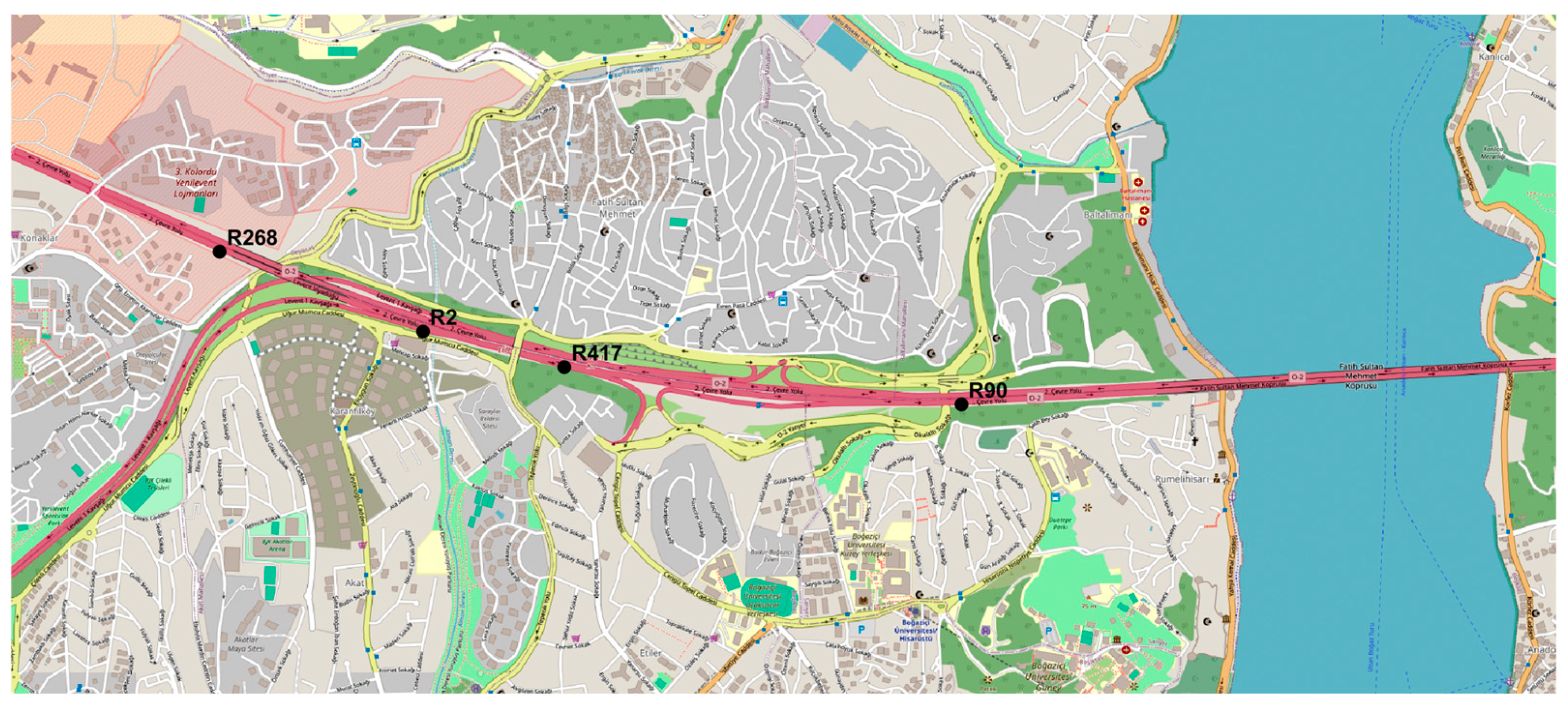
The data consists of time series traffic volumes recorded at 2 min intervals over a 31-day monitoring horizon in October 2022. Data were collected via four RTMSs deployed in a sectional layout along a major arterial corridor on the European side of Istanbul, Turkey. The traffic volume of inbound vehicles approaching the Fatih Sultan Mehmet Bridge toward the Bosphorus crossing was adopted in the present study. This corridor represents a critical high-volume metropolitan artery. To evaluate the performance of the imputation framework under varying operational conditions, each sensor station was analyzed individually (sectional analysis). This method separates the unique missing data profiles, distinctive volume scales, and local geometry effects such as nearby on- and off-ramps that are unique to each monitoring site. The geographic layout of the study area and the spatial distribution of the RTMS stations are illustrated in Figure 1.

3.2. Methodological Workflow and Data Pre-Processing

Before initiating the MI simulations via stochastic regression and PMM-ABB, a rigorous data preparation and diagnostic testing pipeline was established. This pipeline feeds into a multi-domain validation framework to assess the physical structure, temporal preservation, and realism of the imputed traffic streams. The full algorithmic workflow was developed and implemented on the cloud-based MATLAB platform (Version R2026a, MathWorks, Inc., Natick, MA, USA) and its respective statistical and optimization toolboxes. The data preparation phase concentrated on two important tasks: maintaining the continuous 2 min time-step sequence and identifying traffic flow outliers, which are extreme values either due to technical anomalies inherent to the hardware or extreme operational traffic states. From a physical perspective, multi-path radar reflections, environmental signal clutter, or firmware transmission errors can mess up RTMS data. Likewise, heavy traffic can impede the sensor’s ability to separate and identify individual vehicle signatures. To overcome these distortions while maintaining the continuous temporal profile of the dataset, a non-parametric outlier handling procedure based on the Interquartile Range (IQR) was applied to avoid the strict normality assumptions of traditional parametric diagnostics (like the Z-score method). The IQR is a measure of statistical dispersion (mid-spread) and is the difference between the first and the third quartile [47]. Utilizing a modified Winsorized approach, identified anomalies were capped at the upper (Q3 + 1.5 IQR) and lower (Q1 − 1.5 IQR) boundary thresholds, successfully stabilizing the baseline dataset before it was passed to the MI engine [47].

3.3. Missing Data Mechanism Diagnostic

A diagnostic framework for missing data mechanism determination is programmed by a MATLAB (Version R2026a) script. Estimating the missing mechanism is crucial in selecting a proper imputation method. There is no easy way to get valid results about MNAR because it deals with unobserved data, which is unknown. Furthermore, not all imputation methods are suitable for MNAR data and require clear domain knowledge for specific datasets or specialized selection models. On the contrary, MAR data are related to observed data; it is advisable to safely use a multi-imputation method or even simple methods. However, caution is advised in the use of single imputation methods. In our work, the imputation values are derived from an imputation regression model with uncertainty added to the estimated value. On the other hand, in MCAR, no imputation is required; the deletion technique could be used [48,49,50]. The following is the diagnostic protocol for the mechanism of missing data:

A two-sample Kolmogorov–Smirnov test is implemented to compare the empirical distributions of critical time attributes (hour of the day, day of the week) between the two partitions, missing and observed parts, and adopt a p-value to analyze the discrepancy in parameter distributions [49,50]. This test aims to determine whether the missing data is uniformly distributed over time, indicating a MCAR situation, or if the missingness is consistently influenced by timeline scheduling, which supports the MAR mechanism.

Generalized Linear Modeling for MAR Estimation: another supporting test. If the MCAR hypothesis is rejected, the diagnostic protocol then tests if the data meets the conditions for MAR. The relationship is quantified by fitting a Generalized Linear Model (GLM) with logistic regression [51]. The model assumes a binomial distribution for the response variable Ri with a logit link function and is given by Equation (1):

ln (P (R_i = 1)/1 − P (R_i = 1)) = β₀ + β₁(H_i) + β₂(D_i) + β₃(W_i)

(1)

where H_i, D_i, and W_i are the hour of day, day of week, and weekend indicator features respectively. Ri = 1 if the value is missing or Ri = 0 if the value is observed. The estimated predictors (β) are evaluated as significant at 95% confidence level (p < 0.05) [51,52].

Compare means by paired-sample t-test: When temporal distribution or logistic regression tests indicate a temporal pattern of missing data, they cannot distinguish between chronologically scheduled missingness (MAR) and a local sensor’s software glitch resulting from traffic values (MNAR). The t-test employs adjacent boundary state analysis by calculating the average traffic volume for intervals immediately before and after the data-missing block across the entire dataset. This analysis evaluates whether the difference between the two boundary-state arithmetic means significantly deviates from zero. If the traffic volume is stable across the edges of the missing data block, indicating that the loss of data is independent of the traffic state, it can be a sign that the missing data is caused by scheduled resets of the sensor (supporting MAR). Conversely, if the boundaries show statistically significant differences, this indicates an MNAR mechanism. This situation can arise from instantaneous radar blockage or overruns in coverage caused by dense traffic or truck platoons that block the microwave line across several lanes. Or it could be a “snooze” with low traffic volume when the sensor is not collecting data during the late-night hours and only resumes when a continuous, higher traffic volume passes through the monitoring zone.

Heuristic diagnostic screening for MNAR is deployed to evaluate both the local traffic volume states and the temporal contiguity of data dropping. First, an adjacent boundary-value analysis evaluates the traffic volume states immediately bounding each missing window. This step determines whether the data loss is triggered by extreme volumetric states that cause sensor software failure (traffic-dependent MNAR) or if the boundary variations fall within the normal randomness of micro-daily traffic fluctuations. Second, the Consecutive Missing Analysis algorithm quantifies the temporal contiguity of missing blocks to detect prolonged hardware or communication dropouts (infrastructure-driven MAR). These tests will confirm whether the data loss follows an MNAR or will revert us to MAR theory.

Part 1: The Boundary-Context Analysis. The system isolates the values immediately, bounding each missing gap to calculate a local average. By adopting boundary thresholds as a criterion determined by the 10th and 90th percentiles of the global traffic volume dataset, if a non-negligible fraction of the missing sequences is bound by extreme traffic volumes (outside the 10–90% interval), meaning within low-traffic or heavy-traffic states, we have strong empirical evidence of an MNAR mechanism or traffic-driven MNAR.

Part 2: Consecutive Missing Values Analysis: Instead of counting individual sparse missing points, this algorithm looks for contiguous segments of missing data (missing sequences) to determine the length of the sensor disconnection for each failure. The algorithm scans the timeline for the transition boundaries of each data loss, noting the exact start interval when data stops and the correlating end interval when data starts again. By computing the temporal distance between these bounding edges, the algorithm separates each continuous missing block as an individual sequence. This allows for the simultaneous extraction of the maximum uninterrupted missing duration, the average length of missing sequences, and the total length of discrete failure blocks across the monitoring horizon.

3.4. Preliminary Time-Series Diagnostics

Prior to constructing the primary imputation models, a comprehensive preliminary diagnostic framework was executed to extract the structural properties of the traffic telemetry data. The objective of this exploratory phase was to mathematically justify the design of the localized predictor windows, identify dominant seasonal cycles, and assess stationarity to ensure that historical cross-week averaging could be safely adopted without introducing mathematical bias. The diagnostic methodology was conducted through the following sequential phases, using the MATLAB platform:

• Baseline Continuity Preparation (Preliminary Imputation)

Because frequency-domain and autocorrelation functions (ACF) fail on matrices containing missing values, a preliminary non-destructive imputation is executed. Because the sensors are located in the same corridor of the network, we have adopted three sensors’ data out of four that have less and sparse missing values (7.3–11.4%). For every missing index $t$, the algorithm isolates a localized temporal window of $\pm 3$ intervals ($w=3$) and calculates the median value to impute the gap. If it returns NaN (missing), then it will project this window across all available historical and future weeks.

2.

Stationarity and Deterministic Trend Analysis

A critical assumption when utilizing historical median values (such as cross-week, same-time values) is that the dataset does not exhibit severe non-stationary trends. If a strong upward or downward trajectory exists, pulling data from previous weeks systematically underestimates or overestimates current traffic states.

Test 1: Stochastic Trend Testing (Stationary): The Augmented Dickey–Fuller (ADF) test evaluates the presence of a unit root. A loop is initiated starting at differencing order $d=0$. If the test fails to reject the null hypothesis ($p\ge 0.05$), the time series is differenced ($Y\prime =Y_t-Y_{t-1}$), $d$ is incremented by 1, and the test repeats until stationarity is achieved.

Test 2: Deterministic Trend Quantification: The algorithm transforms the temporal dimension into a continuous global index X = [1, 2, 3, …, N], where N is the total number of sequential observations in the dataset, and a linear regression is fitted to the entire temporal horizon. The total longitudinal drift of the dataset is calculated as ${\Delta }_{total}=slope\times N$. The trend is mathematically classified as “negligible” if the absolute total drift is less than half of the global standard deviation of the traffic flow ($\left|{\Delta }_{total}\right|<0.5{\sigma }_Y$) [53,54].

Test 3: Macro-Cyclic Seasonality Extraction:

To empirically determine whether the strongest temporal memory resides in adjacent days or identical historical weeks, the ACF is mapped up to 5500 lags. The algorithm extracts two specific correlation coefficients:

Daily Seasonality ($r_{daily}$): The coefficient exactly at lag 720 (24 h).

Weekly Seasonality ($r_{weekly}$): The coefficient exactly at lag 5040 (7 days).

By executing a programmatic logical check ($r_{weekly}>r_{daily}$), the framework autonomously dictates whether the primary donor search space for the imputation engine should prioritize contiguous daily neighbors or cross-week historical matrices.

Test 4: Local Window Optimization via AIC.

To optimize the size of the localized fallback window for the main predictor, the algorithm identifies the exact number of immediate past intervals that actively influence the current traffic state. The Akaike Information Criterion (AIC) is used to score a sequence of autoregressive models (ARs) from order $\mathrm{p}=1$ to $\mathrm{p}=14$.

For each candidate order p, the log-likelihood ($\ln \left(\mathrm{L}\right)$) of the fitted model is extracted, and the AIC is computed as Equation (2):

$$\mathrm{A}\mathrm{I}\mathrm{C}=2\left(\mathrm{p}+1\right)-2\ln \left(\mathrm{L}\right)$$

(2)

The algorithm loops through all 14 candidate models and selects the AR order p that minimizes the AIC score. This mathematically derived integer defines the exact boundaries of the short-term localized window, balancing predictive power against over-parameterization.

3.5. Traffic Volume Predictor Engineering for Multiple Imputation

This study introduces a custom Profile-Aware Multi-Tier Fallback Heuristic model by extracting seasonal patterns across weeks and rolling localized bounds. Following the mathematical formulation of the multi-tier predictor:

Tier 1: Localized Cross-Week Median: Firstly, the algorithm calculates the median of traffic volume values inside a 14 min local rolling window (±3 intervals or ±6 min) around the target time step; this contributes to reducing the distortion of point-source outliers or minor traffic delays but maintains the short-term profile trends. Secondly, for each of these localized medians, the system identifies all matching historical intervals falling on the exact same time and weekday across a rolling weekly window spanning up to 4 weeks; then, the Tier 1 predictor value is the global median across these valid weeks. This robust macro-historical aggregation acts as a shield in case of unusual traffic behavior; for instance, a particular day may exhibit a major incident or a holiday.

Tier 2: Wider-Window Macro-Historical Median: Should the data density be insufficient to produce Tier 1 within the narrow seasonal window, the algorithm falls back to Tier 2. The core logic is the same, except that the radius of the rolling window is increased to ±15-time steps ±30 min around the historical match interval.

Tier 3: Global Baseline Fallback: In extreme cases where a regional data block is missing throughout the entire 4-week historical archive, the framework resorts to a global baseline value, which corresponds to the unconditional median of all observed traffic volumes within the dataset.

The designed predictor is fundamentally rooted in a structural synthesis of the traditional imputation methodologies outlined in the literature review. It utilizes the exact time-of-day and day-of-week coordinate mapping that serves as the foundation of classical HA methods, but it substitutes the arithmetic mean with the statistical median, ensuring the historical baseline remains highly robust against transient traffic outliers. Traditional Temporal Interpolation fails entirely during prolonged sensor blackouts due to its strict reliance on valid data immediately preceding and following the gap. The engineered predictor captures the mathematical smoothing benefits of Temporal Neighboring by utilizing a localized temporal window ($\pm 3$ to $\pm 15$ min), but it projects this window across historical and future weeks. This allows the predictor to capture localized high-frequency continuity without requiring the immediate chronological data stream to be intact. However, by fusing the cross-week historical anchor (representing global, macro-periodic data) with the expanded temporal search window (capturing local, micro-dynamic data), the multi-tier architecture serves as a direct implementation of the Combined Local–Global methodology.

The last profile predictor is created through a conditional fallback cascade, ensuring a 100% complete feature array without missing values. The built predictor is then incorporated as an independent exogenous covariate within a linear regression framework. The model is trained only on observed, known traffic volumes with respect to their respective predictors. The model takes the optimized regression parameters it just learned from the observed traffic and uses them with the deterministic predictor values to calculate the baseline estimates for the missing traffic. This provides a baseline estimate of the missing traffic flow, with seasonal trends and localized patterns retained in the final MI stage. This hybrid multi-tier approach is a rather robust baseline imputation generator that incorporates the statistical power of nonparametric heuristics as well as the flexibility of the predictive regression models, ensuring no model failure despite extended periods when the sensor is down. The stochastic MI algorithms framework allows the stochastic components of the MI loop to seamlessly inject the required uncertainty, either via randomized draws from an empirically matched discrete donor pool (PMM-ABB) or through stochastic regression imputation. In the latter, a bootstrap step accounts for parametric uncertainty, and fractional Gaussian residual noise is added to preserve natural variance in traffic volumes. This mitigates the risk of the heuristic methods, which directly substitute derived averages, smoothing the timeline and destroying the natural traffic fluctuations.

3.6. Imputation Methods

3.6.1. Multiple Imputation Implementation by Stochastic Linear Regression

To account for both the uncertainty of the model parameters and the inherent stochasticity of traffic flow, a MI framework was executed to generate M parallel completed datasets. The framework utilizes a bootstrap-backed stochastic linear regression architecture optimized via OLS and Gaussian noise addition. The operational pipeline for each imputation instance m executes across three core statistical phases:

Phase 1: Non-Parametric Bootstrapping for Parameter Uncertainty reflects the sample-to-sample variability of the imputation model parameters (the regression coefficients). For each imputation loop, parameter uncertainty is drawn by applying a bootstrap (random sampling with replacement from the observed training data), and the framework mathematically preserves the sampling variance, a core requirement of Rubin’s multi-imputation theory.

Phase 2: Linear Regression: The target traffic volume vector of a sample allocated to train the model (non-masked originally known values) is mapped against its corresponding engineered feature (the cross-week localized median predictor).

Phase 3: Gaussian Residual Noise Insertion.

The model calculates the residuals of the training dataset to obtain its standard deviation, limited by a safety floor to avoid variance collapse. This lower bound functions as an algorithmic fail-safe. During the non-parametric bootstrap resampling stage, random draws with replacement can occasionally generate highly uniform subsamples dominated by zero flow or hyper-stable traffic intervals. Forcing a minimum marginal threshold of 0.1 prevents localized variance collapse within any individual imputation loop (m), ensuring the continuous generation of high-frequency stochastic noise across all runs. A vector of Gaussian noise of the same dimension as the missing data vector is sampled from a standard normal distribution and then scaled directly by the empirical residual standard error. The imputed traffic volume values are obtained by adding the Gaussian noise vector to the predicted value vector from that cross-week median history predictor variable.

3.6.2. Predictive Mean Matching with Approximate Bayesian Bootstrap

In order to preserve the original data distribution and the temporal relationships of the traffic volume data, PMM-ABB was created and embedded within a MI loop to substitute missing values with observed values. The proposed formulation accounts for parametric uncertainty (through bootstrapping) and residual uncertainty (using nearest-neighbor donor matching). The algorithmic pipeline of the proposed implementation of PMM-ABB is carried out in three main stages during each imputation instance m.

Stage 1: Utilizing the deterministic linear regression parameters derived from the bootstrapped training data of the current imputation loop, the algorithm predicts values for both the observed donor data and the missing target data (type 2 matching), mapping both configurations into a unified distance metric space.

Stage 2: Dynamic $K$-Neighbor Autotuning: To optimize the donor pool size, a $K$-nearest neighbor (KNN) search engine operates within the predicted space to find the real observations closest to the missing target based on absolute distance. Crucially, the available candidate donors are restricted entirely to the unmasked training dataset. The hyperparameter $K$ is dynamically tuned inside the loop ($K\in \left\{\mathrm{3,5,10,20,50}\right\}$) using the 20% holdout validation subset strictly as an out-of-sample benchmark. The algorithm evaluates the predictions against this isolated holdout set and automatically adopts the $K$ value that yields the minimum Mean Absolute Error (MAE) for that specific iteration, ensuring no validation data leaks into the donor pool.

Stage 3: Stochastic Donor Selection: The final imputed value is drawn randomly from the optimally tuned, discrete pool of $K$ nearest donors, ensuring variance preservation.

3.6.3. Deterministic Baseline Method Configuration: Historical Average Imputation

To rigorously map the predictive boundaries of the proposed stochastic MI frameworks, their performance was evaluated against a highly competitive, deterministic baseline. To execute this comparative evaluation, the dataset was formally partitioned: a random 20% subset of the known, valid traffic observations was artificially masked to serve as the ground-truth test set. Model accuracy was subsequently quantified by calculating the residuals, the absolute differences between the algorithmically imputed predictions for these masked intervals and their real, observed values. Furthermore, rather than relying on a singular, fragile heuristic, this baseline was explicitly engineered with a multi-tier fallback hierarchy to prevent computational collapse under severe telemetry failure, ensuring a robust and fair comparison against the advanced MI models.

Primary Imputation Logic (Classical HA): The primary mechanism of the algorithm is designed to capture macro-seasonal daily traffic waves, aligning with standard HA heuristics. For any target missing value occurring at a specific time slot (t) on a specific day of the week (d), the algorithm strictly scans the unmasked training observations to prevent validation leakage. It identifies all identical time–day combinations ($\mathrm{t},\mathrm{d}$) across the available historical weeks and calculates the arithmetic mean, ignoring any concurrent missing values; see Equation (3):

$${\stackrel{\mathrm{ˆ}}{\mathrm{y}}}_{\mathrm{t},\mathrm{d}}={\displaystyle \frac{1}{{\mathrm{N}}_{\mathrm{t}\mathrm{r}\mathrm{a}\mathrm{i}\mathrm{n}}}}{\displaystyle \sum _{\mathrm{k}=1}^{{\mathrm{N}}_{\mathrm{t}\mathrm{r}\mathrm{a}\mathrm{i}\mathrm{n}}}}{\mathrm{y}}_{\mathrm{t},\mathrm{d},\mathrm{k}}$$

(3)

where ${\stackrel{\mathrm{ˆ}}{\mathrm{y}}}_{\mathrm{t},\mathrm{d}}$ represents the estimated baseline traffic volume for time slot (t) on day of the week (d), ${\mathrm{N}}_{\mathrm{t}\mathrm{r}\mathrm{a}\mathrm{i}\mathrm{n}}$ is the total number of available historical weeks in the unmasked training dataset, and ${\mathrm{y}}_{\mathrm{t},\mathrm{d},\mathrm{k}}$ is the actual observed traffic volume at that exact time slot and day during historical week k.

Adaptive Fallback Mechanisms: Recognizing that strict historical matching fails during massive missingness (where historical donor weeks are completely starved of data), the baseline algorithm is equipped with two sequential fail-safes:

Tier 1 (Temporal Closest-Neighboring Fallback): If the primary historical match returns an empty set, the algorithm shifts from cross-week matching to localized sequential tracking, incorporating the principles of Temporal Closest-Neighboring methods. It dynamically scans backward in time from the missing point to isolate up to the last seven valid, unmasked observations. Because the network records data in 2 min intervals, this effectively averages the last known 14 min of physical traffic flow prior to the blackout, preserving the immediate localized physical inertia of the traffic shockwave.

Tier 2 (Ultimate Global Fail-Safe): In extreme boundary cases where localized historical data is completely unavailable, specifically if a massive blackout occurs at the absolute beginning of the recorded dataset, the 14 min backward scan will return empty. In this isolated scenario, the algorithm triggers its ultimate fail-safe, imputing the global arithmetic mean (${\mu }_{global}$) of the entire unmasked training dataset to guarantee the pipeline does not mathematically crash.

3.7. Multiple Imputation Dynamic Loop

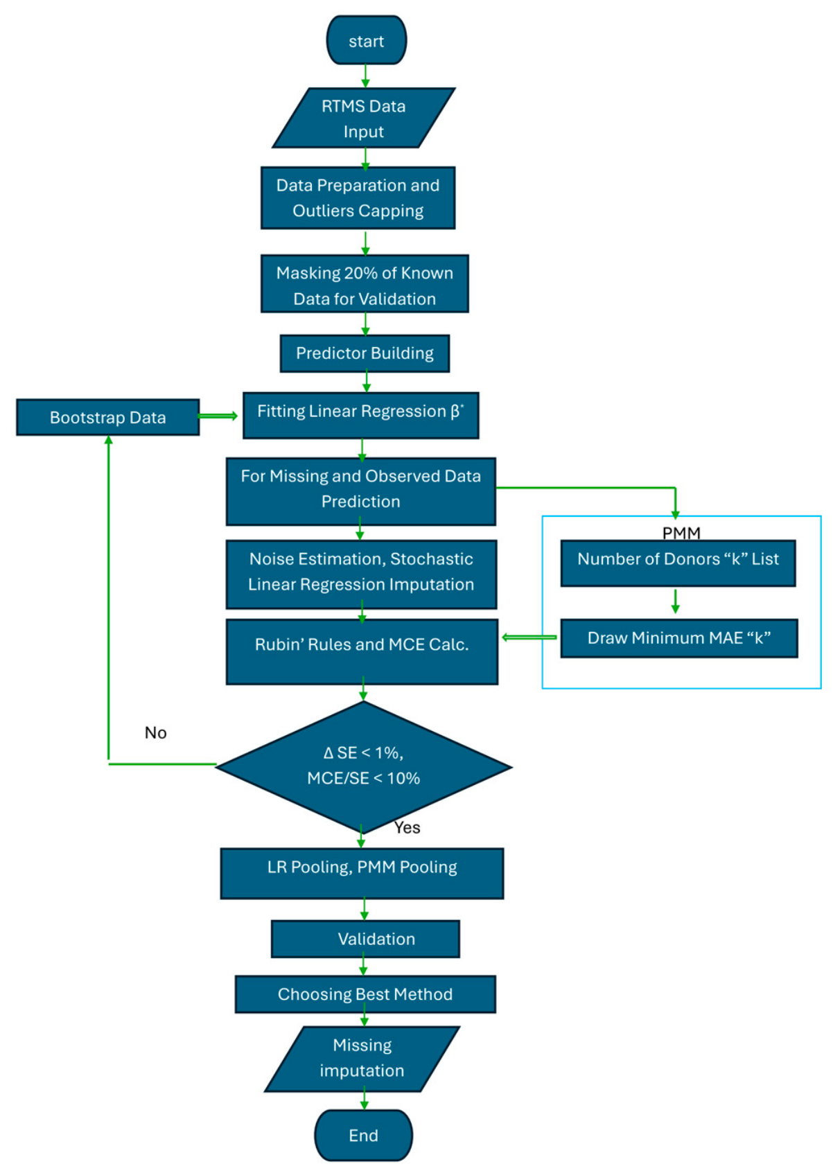
The entire imputation framework is implemented using sophisticated MI procedural architecture. Instead of pre-setting the number of imputations (M), the system evaluates statistical convergence dynamically. The process alternates between stochastic parameter updates and local out-of-sample optimization, continuing until the standard error variance stabilizes and the simulation noise drops below standard academic thresholds. See Figure 2, which explains the dynamic imputation framework. The imputation framework progresses in blocks of 5 loops of imputations, with a maximum of M = 250. Inside each individual imputation loop, the parameters are updated by applying a Bayesian bootstrap to the observed data.

Two statistical metrics are evaluated as criteria to check convergence at every step (M = 5).

Criterion A: Rubin’s Rule Cumulative Standard Error Stability: The total standard error ($\mathrm{S}\mathrm{E}=\sqrt{\mathrm{T}}$) is used to detect system stability, which occurs when the relative change in the cumulative standard error between consecutive assessed blocks, as shown in Equation (8), falls below a specified threshold. Operationalizing Blazek et al.’s [38] requirement for standard error stability, we empirically set the change threshold at 1% because it perfectly synchronizes with the Monte Carlo Ratio—preventing the premature termination seen at 5% and the computational exhaustion of 0.5%.

The total variance T of the imputed datasets represents both the within-imputation variance U and the between-imputation variance B, see following Equations (4)–(7) [28].

$$\overline{\mathrm{\theta }}={\displaystyle \frac{1}{\mathrm{M}}}{\displaystyle \sum _{\mathrm{i}=1}^{\mathrm{m}}}{\widehat{\mathrm{\theta }}}_{\mathrm{i}}$$

(4)

$$\overline{\mathrm{U}}={\displaystyle \frac{1}{\mathrm{m}}}{\displaystyle \sum _{\mathrm{i}=1}^{\mathrm{m}}}{\mathrm{U}}_{\mathrm{i}}$$

(5)

$$\mathrm{B}={\displaystyle \frac{1}{\mathrm{M}-1}}{\displaystyle \sum _{\mathrm{i}=1}^{\mathrm{M}}}{\left({\widehat{\mathrm{\theta }}}_{\mathrm{i}}-\overline{\mathrm{\theta }}\right)}^2$$

(6)

$$\mathrm{T}=\overline{\mathrm{U}}+\left(1+{\displaystyle \frac{1}{\mathrm{m}}}\right)\mathrm{B}$$

(7)

$${\delta }_{SE}=\left|{\displaystyle \frac{S{E}_{current}-S{E}_{preceding}}{S{E}_{preceding}}}\right|\times 100\%$$

(8)

where M is an imputation number, ${\widehat{\mathrm{\theta }}}_{\mathrm{i}}$ is arithmetic mean of imputation dataset point estimates, and $\overline{\mathrm{\theta }}$ and $\overline{\mathrm{U}}$ are the mean of the accomplished imputations of ${\widehat{\mathrm{\theta }}}_{.}$ and U respectively.

Criterion B: MCE: Under the reproducibility argument, Monte Carlo simulation stability is achieved as its error value (Equation (9)) [45] drops below 10% of the standard error of point estimates at any check block of imputation loops. Equation (10) shows the Monte Carlo ratio, which was adopted in the current study as one of the convergence measurements:

$$\mathrm{M}\mathrm{C}\mathrm{E}=\sqrt{{\displaystyle \frac{\mathrm{B}}{\mathrm{M}}}}$$

(9)

$$\mathrm{M}\mathrm{C}\mathrm{R}=\left({\displaystyle \frac{\mathrm{M}\mathrm{C}\mathrm{E}}{\mathrm{S}\mathrm{E}}}\right)\times 100\%$$

(10)

In return to the previous studies stated in the literature [41,45,55], adopting efficiency as a common measurement to tune the imputation cycles, we are here calculating these parameters to study, like FMI, RE, and loss in power (P_L), as illustrated below in Equations (11), (12), and (13), respectively.

$$\mathrm{F}\mathrm{M}\mathrm{I}={\displaystyle \frac{\mathrm{B}}{\left(\mathrm{B}+\mathrm{U}\right)}}$$

(11)

$$\mathrm{R}\mathrm{E}={\left(1+{\displaystyle \frac{\mathrm{F}\mathrm{M}\mathrm{I}}{\mathrm{M}}}\right)}^{-1}$$

(12)

$${\mathrm{P}}_{\mathrm{L}}={\displaystyle \frac{\mathrm{F}\mathrm{M}\mathrm{I}}{\mathrm{M}}}$$

(13)

To evaluate statistical efficiency and determine the optimal termination point of the MI cycles, three standard metrics were defined and calculated: Rubin (1987) [28], Graham et al., and Bodner [41,44]:

FMI: Unlike the raw percentage of missing data, FMI defines the true proportion of the total sampling variance that is directly attributable to the uncertainty caused by the missing values.

RE: This metric defines the efficiency of the point estimates achieved with the current finite number of imputations ($M$) relative to the theoretical ideal of infinite imputations. An RE approaching 1.0 indicates that generating additional datasets will not meaningfully improve the precision of the estimates.

${\mathrm{P}}_{\mathrm{L}}$: The statistical power for hypothesis testing represents the statistical power penalty incurred by utilizing a finite $M$ instead of an infinite number of imputation loops.

As the system converges to the specified threshold, it stops with the optimal number of imputations. For each of the imputation methods, the arithmetic mean was calculated across all iterations for each individual missing gap.

3.8. Multi-Domain Validation Metrics

After assigning values to missing gaps using two datasets with two imputation methods, a series of validation strategies were conducted to figure out the performance of the proposed predictor within both imputation methods, as well as the imputation methods’ comparative performance and accuracy. These methods indicate that performance varied among predictive accuracy, temporal dependency preservation, and the preservation of realism or physical traffic characteristics in the data.

3.8.1. Random Holdout Validation

This test is used to evaluate the localized point-prediction accuracy of the MI framework. Using a fixed-seed random permutation algorithm to ensure deterministic reproducibility, the system partitions 20% of the known, observed traffic counts to serve as an independent evaluation subset (ground truth) or testing set. This testing set is then artificially masked by converting its elements to NaN (Not-a-Number) values in the active dataset, thus extending the total operational missingness to include both the original field gaps and the newly masked validation vectors. The rest of the known, observed data (80%) is used as the training matrix for fitting the baseline linear regression model and building the candidate neighborhood donor space in the PMM-ABB steps. This strict partitioning guarantees zero data leakage; the regression parameters and the historical median predictor are derived exclusively from the 80% training matrix, leaving the artificially masked 20% strictly as an independent ground-truth baseline. The performance is then evaluated using the MAE, Root Mean Squared Error (RMSE), and Coefficient of Determination R² (over the held-out evaluation indices) by directly comparing the imputed values with their actual observed ground-truth counterparts (serving as a validation benchmark).

3.8.2. Temporal Cross-Validation

Although the holdout validation provides an independent estimate of localized accuracy, it is not an exact copy of predictive deployments over continuous time horizons. To study this, a temporal leave-one-week-out cross-validation approach was used. This mechanism assesses the robustness of the imputation models under systemic block-missingness over time, and the model parameters are well generalized to different temporal blocks. Bergmeir et al. [56] suggest the application of block cross-validation out of all types of cross-validations for the purposes of time series evaluation, which then becomes the standard procedure. In the current study, “blocks” have been delineated by chronological considerations of real-world calendars as weeks, making it a temporal block cross-validation. The temporal validation procedure operates as an external validation loop that is executed independently for each imputation cycle. The observed data time series is discretely partitioned into week blocks to represent the set of weekly intervals, and the algorithm operates strictly on non-missing data; it exchanges a hidden week (the testing week) for each iteration across the weeks with the training weeks. The observations of the testing week were originally known prior to validation masking, which will be utilized as ground truth to evaluate the prediction accuracy. Then, on the training subset data (engineered predictor data and target data), the linear regression model was trained and used to estimate values for the artificially masked data. By artificially masking the entire testing week prior to execution, the multi-tier historical predictor is forced to derive its local and macro-medians exclusively from the remaining unmasked training weeks. This enforces strict chronological isolation, ensuring the framework reconstructs the temporal block without any illicit mathematical access to the target week’s native data. To measure overall predictive performance under a block-missingness approach, we use Temporal Cross-Validation Mean Absolute Error (T-CV-MAE) and Root Mean Squared Error (T-CV-RMSE) of the residuals. We then averaged the results from all weeks to evaluate performance over time. In this test, we do not evaluate random scattered data; instead, we check if the long consecutive intervals or days were missing.

3.8.3. Temporal Integrity Validation by Using ACF

Conventional point-prediction metrics, such as MAE and RMSE, are effective at measuring individual distance errors, but they do not account for sequential dependencies. In time-series traffic data, it is just as important to keep the natural cycles and seasonal changes as it is to reduce point-by-point errors. Focusing only on point errors can unintentionally smooth out the data, removing daily patterns in traffic flow. To guarantee that the proposed predictor within the dynamic-stop MI framework preserves the temporal structure of the traffic data, this study utilizes an ACF as a validation test. The ACF measures the linear correlation of a time series with a lagged version of itself in a given lag interval (h). Equation (14) exhibits the mathematical expression of the autocorrelation coefficient (ρ) at lag h:

$${\rho }_h={\displaystyle \frac{{\sum }_{t=1}^{N-h}\left(y_t-\overline{y}\right)\left(y_{t+h}-\overline{y}\right)}{{\sum }_{t=1}^N{\left(y_t-\overline{y}\right)}^2}}$$

(14)

$$\mathrm{A}\mathrm{C}\mathrm{F}-\mathrm{M}\mathrm{A}\mathrm{E}={\displaystyle \frac{1}{720}}{\displaystyle \sum _{\mathrm{h}=1}^{720}}\left|{\mathrm{E}}_{\mathrm{h}}\right|$$

(15)

$$\mathrm{A}\mathrm{C}\mathrm{F}-\mathrm{R}\mathrm{M}\mathrm{S}\mathrm{E}=\sqrt{{\displaystyle \frac{1}{720}}{\displaystyle \sum _{\mathrm{h}=1}^{720}}{\left({\mathrm{E}}_{\mathrm{h}}\right)}^2}$$

(16)

where $\overline{y}$ represents the series data average, N is the total number of observations, and Y is time series data. As the traffic is recorded at 2 min intervals (equating to 720 observations a day) and to evaluate the preservation of daily fluctuations, the algorithm is tuned to track a lag boundary of h (720), where the seasonal pattern of traffic is the strongest. First, the algorithm imputes the originally missing gaps with zeros, creating a pad for baseline comparisons, so the comparison will be based on the estimated signals that replace the artificially hidden values (the randomly selected 20% from the hold-out validation) and their ground-truth signal. In this way, we preserve the time-series real-world length. Secondly, the algorithm calculates autocorrelation coefficients for both series sequences of 720 coefficients (lag 1 to lag 720) using Equation (14) to facilitate getting the daily coefficients (target lag). In more detail, it spans the entire 31-day data set to produce an overall average correlation of any given 24-h period with the next inside the cycle. Finally, we use Equations (15) and (16) to evaluate the distance between the two temporal sequences. All the calculations are repeated with each imputation iteration and end with the reporting of average ACF_MAE and ACF_RMSE of all the imputation loops, which quantify the deviation in the temporal data using absolute and squared error metrics, respectively, and provide an indication of “how well” the reconstructed temporal sequences replicate the dynamic behavior of the real-world traffic in the network.

3.8.4. Frequency-Domain Spectral Validation

Time-domain metrics (like MAE and RMSE) measure localized tracking errors; they tend to fall short in reflecting the presence of macro-level temporal periodicity structures and high-frequency white noise in the traffic time series. We conduct a frequency-domain validation framework using non-parametric spectral density estimation in order to check if localized traffic periodicities are properly maintained (the daily and weekly patterns) with no structural distortion. The continuous volume timeline of the recorded over 31 days of traffic data (at 2 min intervals) is mapped from the time domain into the frequency domain through a periodogram using Fast Fourier Transform (FFT) to estimate the Power Spectral Density (PSD) [57,58,59,60]. This validation method falls into 4 distinct steps; before transforming the signals, it is critical to isolate the spectral evaluation strictly to the independent testing partition. To ensure strict statistical independence and avoid confounding the spectral comparison with originally missing telemetry, any native data gaps (sensor failures existing prior to the 20% artificial validation masking) are forcefully zero-padded in both the ground-truth array and the imputed array [61,62,63,64]. For massive multi-day blackouts, such as the failure at Sensor R417, this zero-padding ensures that the originally unobserved voids are entirely excluded from the performance metric calculations. Consequently, the high-fidelity spectral validation scores reflect the model’s accuracy exclusively over the successfully held-out real data points, entirely separating the structural predictor from the physical validation reference. To transform the time-domain metrics into a macro-structural evaluation, the following signal-processing definitions were operationalized:

Discrete Fourier Transform (DFT): The mathematical operation that converts the continuous time-domain sequence of traffic volumes into the frequency domain. It decomposes the traffic stream into its underlying cyclic components, revealing the specific amplitude and phase of repeating sinusoidal waves (e.g., daily commuter influxes).

PSD: A definitive measure that quantifies how the true physical energy (or variance) of the traffic signal is distributed across these different frequency bands. It identifies the dominant periodicities without being skewed by localized, high-frequency time-domain noise.

Because these native gaps are identical in both vectors, they mathematically cancel out in the comparative analysis.

Step 1: Transform time to frequency: Traffic data is considered a discrete-time signal; the sampling interval (∆t) = 2 min = 120 s; the sampling frequency can be Fs = 1/∆t or Fs = 1/120, approximately 0.00833 Hz.

Step 2: Discrete Fourier Transform (DFT) and PSD: The continuous traffic observations are transferred into the frequency domain using the FFT protocol. First, the complex DFT coefficients, $X\left(f\right)$, are calculated for both the true validation series and the imputed series over all frequencies up to the Nyquist limit (Fs/2) using Equation (17). Subsequently, the PSD $P\left(f\right)$, which represents the true signal energy at a specific frequency, is calculated using the periodogram estimate; see Equation (18):

$$X\left(f\right)={\displaystyle \sum _{t=1}^N}{y}_t{e}^{-j2\pi ft}$$

(17)

$$P\left(f\right)={\displaystyle \frac{1}{N\cdot F_s}}{\left|X\left(f\right)\right|}^2$$

(18)

where $N$ is the total number of temporal observations, $y_t$ is the traffic volume at time index $t$, $f$ is the specific frequency variable being evaluated (Hz), and $j$ is the imaginary unit $\sqrt{-1}$. P(f) is the power spectral density at specific frequency f; it could be an observed signal (P(f) original) or imputed signal (P(f) imputed). Here, the signal is analyzed using complex numbers, where each number denotes the amplitude and phases of different sinusoidal waves.

Step 3: Distance Evaluation Metrics: To assess the distance between the true energy (P orig) and imputed (P imp) profiles through the whole frequency spectrum, three distinct assessment metrics are calculated at each imputation loop: MAE, RMSE, and normalized spectral similarity. These are standardized errors relative to the mean energy (power) of the original signal in Formulas (19), (20), and (21), respectively:

$${\mathrm{Spectral}\_\mathrm{MAE}}_m={\displaystyle \frac{1}{K}}{\displaystyle \sum _{k=1}^K}.\left|10{log}_{10}{P}_{\left(\mathrm{imp},m\right)\left(f_k\right)}-{10{log}_{10}P}_{\mathrm{orig}\left(f_k\right)}\right|$$

(19)

$${\mathrm{Spectral}\_\mathrm{RMSE}}_m=\sqrt{{\displaystyle \frac{1}{K}}{\displaystyle \sum _{k=1}^K}{\left(10{{\log }_{10}P}_{\mathrm{imp},m}\left(f_k\right)-10{{\log }_{10}P}_{\mathrm{orig}}\left(f_k\right)\right)}^2}$$

(20)

$$Spe{c}_{Si{m}_{Nor{m}_m}}={\displaystyle \frac{\sqrt{\left(\frac{1}{K}{\displaystyle {\sum }_{k=1}^K}.{\left(P_{\left(\mathrm{imp},m\right)\left(f_k\right)}-P_{\mathrm{orig}\left(f_k\right)}\right)}^2\right)}}{\frac{1}{K}{\displaystyle {\sum }_{k=1}^K}.P_{\mathrm{orig}\left(f_k\right)}}}$$

(21)

A lower normalized spectral similarity value reveals how the imputation process accurately mirrors human behavior and physical vehicle flow.

Step 4: The final reported spectral metrics represent average metrics across all MI loops.

3.9. Non-Parametric Empirical Percentile Confidence Intervals

To rigorously quantify the statistical reliability and the true underlying data variance for all multi-domain validation metrics (Holdout, Temporal-CV, Autocorrelation, and PSD), 95% confidence intervals were constructed using a non-parametric empirical percentile bootstrap methodology [65,66,67,68].

Traditional parametric confidence intervals rely on the standard error of the mean, which artificially shrinks toward zero as the number of imputation iterations ($M$) increases. Additionally, standard parametric methods assume a perfect Gaussian distribution, which is mathematically inappropriate for strictly non-negative or skewed error distributions, such as absolute residuals and logarithmic spectral densities. To overcome these limitations and accurately capture the true variance of the physical traffic data, this study extracts the confidence bounds directly from the empirical distribution of the iterative validation results.

For each validation metric evaluated across the $M$ imputation cycles dictated by the dynamic stopping algorithm, a complete distribution vector of the metric ($\mathrm{V}$) is generated (${\mathrm{V}}_{MAE}=\left[MA{E}_1,MA{E}_2,\dots ,MA{E}_M\right]$). The 95% confidence interval (CI) boundaries are extracted by isolating the 2.5th and 97.5th percentiles of this empirical vector to determine the lower and upper bounds of the confidence interval respectively. By applying this non-parametric percentile engine, the resulting confidence intervals do not suffer from simulation-induced standard error shrinkage. Instead, they provide highly stable, data-driven uncertainty margins that represent the true empirical variance and robustness of the MI models across the entire evaluation horizon.

3.10. Evaluation Metrics and Standardized Effect Size (Cohen’s d)

The performance of the proposed MI frameworks (Stochastic Regression and PMM-ABB) is rigorously evaluated against the deterministic historical baseline (HA) using standard aggregate metrics such as MAE.

However, simple aggregate metrics do not quantify the statistical magnitude of improvement relative to the natural volatility of traffic flow. To address this, Cohen’s d was employed to measure the standardized effect size of the error reduction [69,70,71,72]. In the context of MI, evaluating Cohen’s $d$ based on the variance of the summary metrics across $M$ imputation loops produce artificially inflated values, as the standard error of the mean approaches zero upon algorithm convergence.

To provide a physically meaningful measure of model diagnostic improvement, this study utilizes a micro-residual evaluation methodology. In this approach, Cohen’s $d$ is calculated by comparing the full empirical distributions of the absolute prediction errors (residuals) at the individual observation level. For a deterministic baseline model (HA), the absolute error (e) for a test observation $i$ is defined as Equation (22):

$$e_{baseline,i}=|Y_{imputed,i}-Y_{actual,i}|$$

(22)

For the stochastic MI models, absolute errors are aggregated across all $N_{test}$ evaluation observations and all $M$ imputation iterations to capture the complete predictive uncertainty; see Equation (23). This creates a pooled residual array of size $n_1=M\times N_{test}$:

$$e_{model,i,m}=|Y_{imputed,i,m}-Y_{actual,i}|$$

(23)

The average of these pooled error distributions ($\mu$) inherently aligns with the overall MAE of the model. To evaluate the effect size between a proposed model (${\mu }_1$) and the baseline (${\mu }_2$), the unbiased sample variance of the absolute errors ($s^2$) is computed for both distributions. The pooled standard deviation ($s_{pooled}$) of the prediction errors is then calculated as a weighted average based on their respective sample sizes ($n_1$ and $n_2$), as illustrated in Equation (24):

$$s_{pooled}=\sqrt{{\displaystyle \frac{\left(n_1-1\right)s_1^2+\left(n_2-1\right)s_2^2}{n_1+n_2-2}}}$$

(24)

Finally, the standardized effect size of the error reduction is quantified using Cohen’s $d$; see Equation (25):

$$d={\displaystyle \frac{{\mu }_1-{\mu }_2}{s_{pooled}}}$$

(25)

By utilizing the standard deviation of the individual absolute residuals rather than the standard error of the simulation loop means, the resulting Cohen’s $d$ mathematically grounds the model’s accuracy improvement within the real-world variance of daily traffic measurements. A negative Cohen’s $d$ value indicates that the proposed stochastic model successfully reduced the absolute residual errors compared to the baseline method. Standard interpretation thresholds were applied: $\left|d\right|\approx 0.2$ denotes a small effect, 0.5 a medium effect, and ≥0.8 a large and highly significant practical effect. This methodology was systematically applied across all four validation domains: holdout validation, temporal block cross-validation, ACF lag deviation, and PSD decibel deviation.

4. Results and Discussion

4.1. Missing Data Mechanism

The data collected along the bridge approach were divided into four segments based on the locations of the RTMS sensors. We analyzed each segment of data individually. The raw data tables contained duplicate rows, and some had gaps in the time-sequence data, which included intervals with missing data as well as outliers. All of these issues were dealt with to prepare the data for imputation and subsequent analyses. In the context of outliers, we detected anomalies of less than 0.5% across all segments, which were conditionally capped with lower bounds. However, missing mechanisms are also crucial for MI processes. Distributions of both time attributes (hour of the day and day of the week) of the two partitions, missing and observed parts, using the Kolmogorov–Smirnov test show p = 0.000 for all sensors’ data; this is a statistically significant result (p < 0.05) that rejects H₀ (there is no statistical difference), which leads to the conclusion that they are not uniformly distributed over time attributes and the mechanism is associated with temporal patterns, not MCAR. Nevertheless, we fitted a generalized linear model to the data to confirm the mechanism of missing values. We observed that the significance p-value is less than 0.05 for all temporal attributes’ coefficients of all data (see

Table 3. The Missing Mechanism Diagnostic Results.

Sensor ID	Missing %	Average Consecutive Interval Missing	Max. Consecutive Interval Missing	Hour of Day Coefficient	Weekend Coefficient	Day of Week Coefficient
R268	11.4	5 (10 min)	453 (15 h)	−0.0113 (p = 0.0000)	−1.0350 (p = 0.0000)	0.04 (p = 0.0003)
R90	7.3	4.5 (9 min)	582 (19.4 h)	−0.0173 (p = 0.0000)	−1.0728 (p = 0.0000)	0.0683 (p = 0.000)
R2	8.7	3 (6 min	222 (7.4 h)	0.0642 (p = 0.0000)	−0.2592 (p =0.0000)	−0.0366 (p = 0.0044)
R417	88.9	15 (30 min)	3003 (100 h)	0.0158 (p = 0.0000)	0.5397 (p = 0.0000)	−0.0843 (p = 0.0000)

), and the chi-squared statistic against the constant model is high, with a p-value less than 0.05. This indicates that the missing values are related to time, confirming that the missing data mechanism is MAR and complying with the criteria of Little (1988) and Rubin (1976) [7,31] to implement MIs. The missingness could be attributed to routine daily maintenance, software scheduling cycles, or automated daily sensor reboots. At the same time, there is a possibility of missing data being associated with traffic state, such as a local sensor’s software glitch due to traffic values being MNAR during peak hours or in the case of low traffic volume where the sensor stalls and resumes when traffic levels return to normal.

However, we conducted a t-test to compare the average traffic volume before and after the missing data interval. The results reveal that there is no significant difference across the boundaries, as shown by a p-value greater than 0.05 for sensors (R268, R90, R417). This means that the traffic flow is moving normally over the missing data boundaries. On the contrary, the traffic near the sensor (R2) shows a significant change across the missing edges (p-value = 0.009), which supports a data-driven MNAR case. To augment our confidence in this finding, we calculated the fraction of missing sequences that fell outside (10–90%) of the global traffic volume dataset. We found that the fraction of missing data surrounded by extreme values was less than 5% for all sensors, including R2, while 95% of the missing data was under a normal traffic volume state. This result rules out the data-driven MNAR case. However, the analysis of consecutive missing data revealed that the system recorded between 360 and 1313 missing sequences, with maximum consecutive missing data intervals ranging from 222 to 3003-time steps. This pattern of massive, continuous blockage does not reflect volume-triggered sensor glitches (MNAR) or normal traffic fluctuations. Therefore, we conclude that these extensive data voids are driven by prolonged infrastructure dropouts and equipment failures. Because these hardware failures occur independently of the actual physical traffic volume on the road, the missing data mechanism strictly satisfies the criteria for MAR. Consequently, this confirms that the historical cross-week temporal trends remain mathematically uncorrupted and validate the use of the MI framework.

Consequently, the culmination of these diagnostic tests confirms that the RTMS sensors are completely decoupled from the physical traffic state. The data loss is strictly driven by external factors ranging from routine network maintenance and scheduled sensor resets to severe, multi-day hardware and communication failures. Because the missingness operates independently of the actual traffic flow, the underlying historical patterns and cross-week temporal trends remain mathematically uncorrupted, providing a statistically valid foundation to reconstruct the missing blocks. Furthermore, while the average missing interval spans a manageable 6 to 30 min, the maximum consecutive gaps extend from several hours to over four days (e.g., 100 h at Sensor R417). This extreme variability definitively dictates the necessity of the engineered adaptive Tier-2 wide window (±15 steps/±30 min). By dynamically expanding the cross-week search horizon, the framework guarantees the extraction of a stable, variance-protected historical baseline even during the most prolonged sensor disconnects.

4.2. Pre-Modeling Diagnostics

Structural diagnostic testing is crucial to perform on baseline data with rigor before historical parameters are passed to the stochastic MI engine. This phase ensures that base temporal features, particularly stationarity, trend intensity, and seasonal dominance, are clearly mapped. These tests prevent structural misspecification in the subsequent imputation stages.

• Testing for Strict Stochastic Stationarity: Augmented Dickey–Fuller testing indicates no need for differencing (d = 0). The test gave satisfactory ADF statistics, which correspond to a very significant p-value less than 0.05 for the tested sensors’ data. This provides empirical evidence that the traffic signal is a purely stationary process over the monthly monitoring frame. Thus, the mean, variance, and autocovariance of the flow rates are steady throughout time, and no risk of statistical drift is encountered in many imputation loops.
• Measuring the Intensity of Trend: The long-term trend analysis over the continuous timeline provided a very tiny linear slope. This empirical conclusion verifies our assumption of seasonal equilibrium, confirming that the data is not subject to long-term structural demand inflation or deflation during the month.
• Dominant Seasonality and Information Architecture Isolation: Autocorrelation coefficient results show that the daily structural cycle is slightly higher than the weekly cycle. Finally, the automated AIC information sweeps across 14 discrete lag spaces, identifying that the optimal AR (autoregressive) order is exactly 10 lags. The result shows that the short-term stochastic background noise of the traffic flow has an active physical memory span of 20 min. These empirical results prompted us to develop the “Cross-Week” seasonal median predictor; the utilization of a localized cross-week smoothing window of ±3 intervals (6 min) around the target missing timestamp is perfectly scaled. It captures local variance and does not smooth high-frequency waves in traffic.

4.3. Predictor Engineering

The traffic data were recorded from different locations along the road using four sensors. After data cleaning, four datasets were prepared, and we engineered the predictors to work with each dataset separately. During the empirical evaluation of the corridor’s data stream, a high block-missingness severely exhausted the localized historical data points. In these worst-case scenarios, the framework successfully deployed its Tier 2 search contingency, expanding the localized window from the baseline ± 3 steps to an operational width of ±15 time steps. This wider temporal scope effectively mitigated localized micro-variants across the adjacent weeks, providing a stable, variance-protected data structural foundation that enables the MI engine to completely reconstruct the extensive data gaps, which explains why we could not use standard Holt–Winters or SARIMA. Our predictor adaptively expands its window to look broadly into the surrounding weeks to pull uncorrupted traffic profiles.

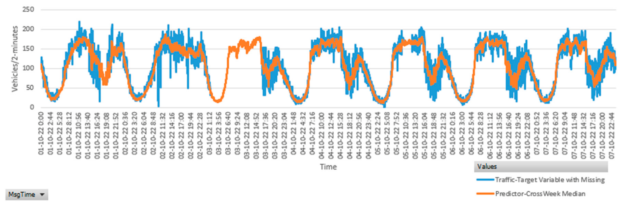
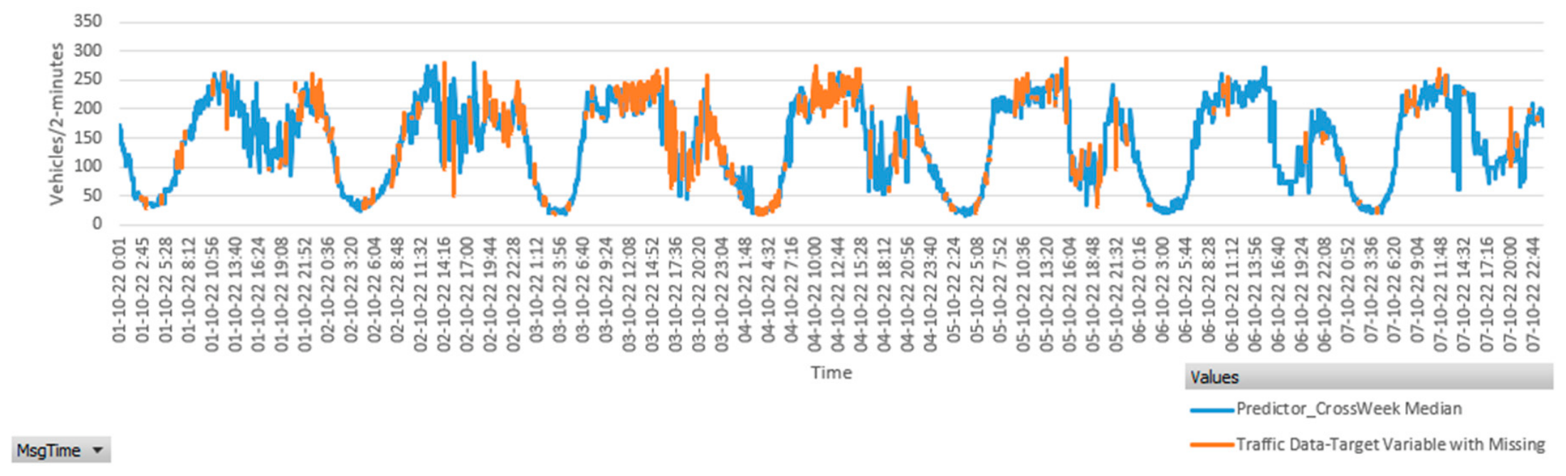
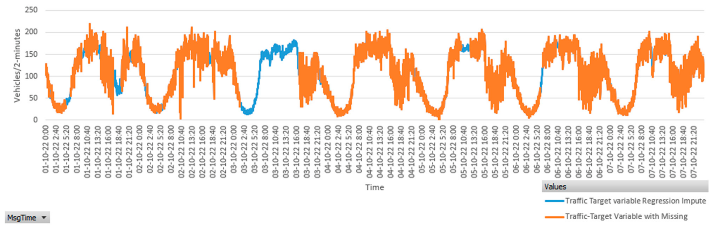
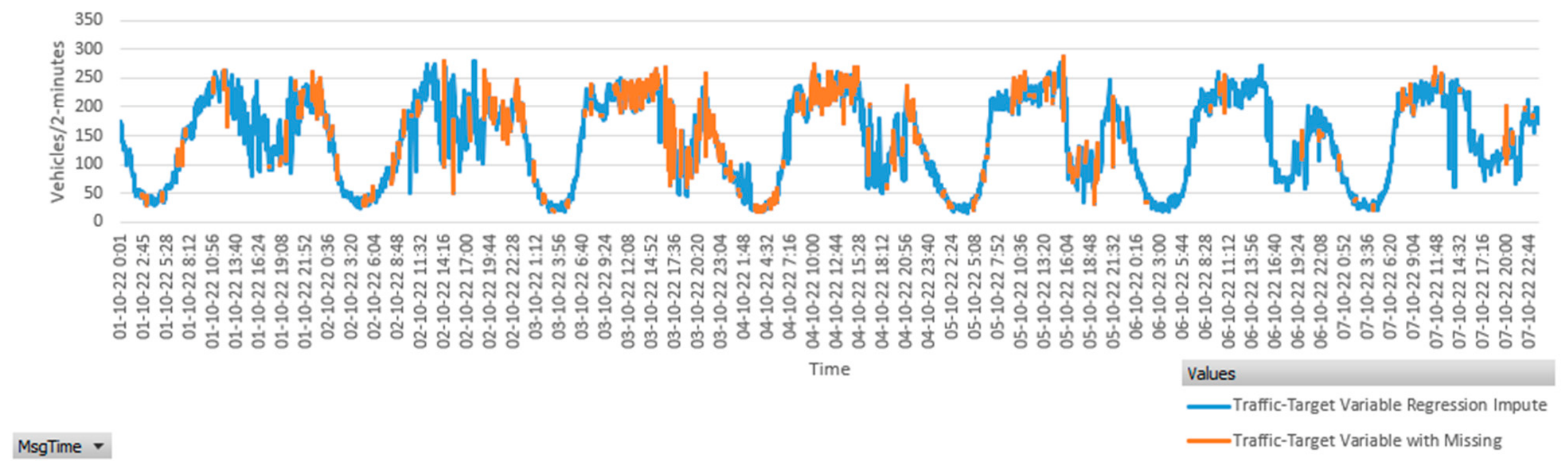
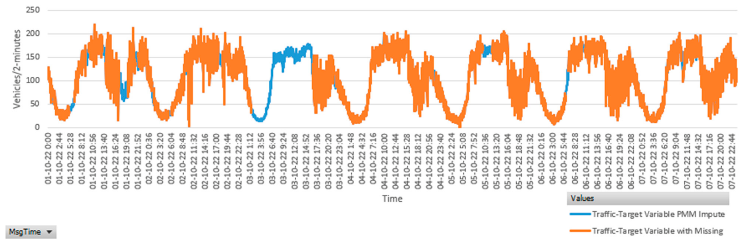
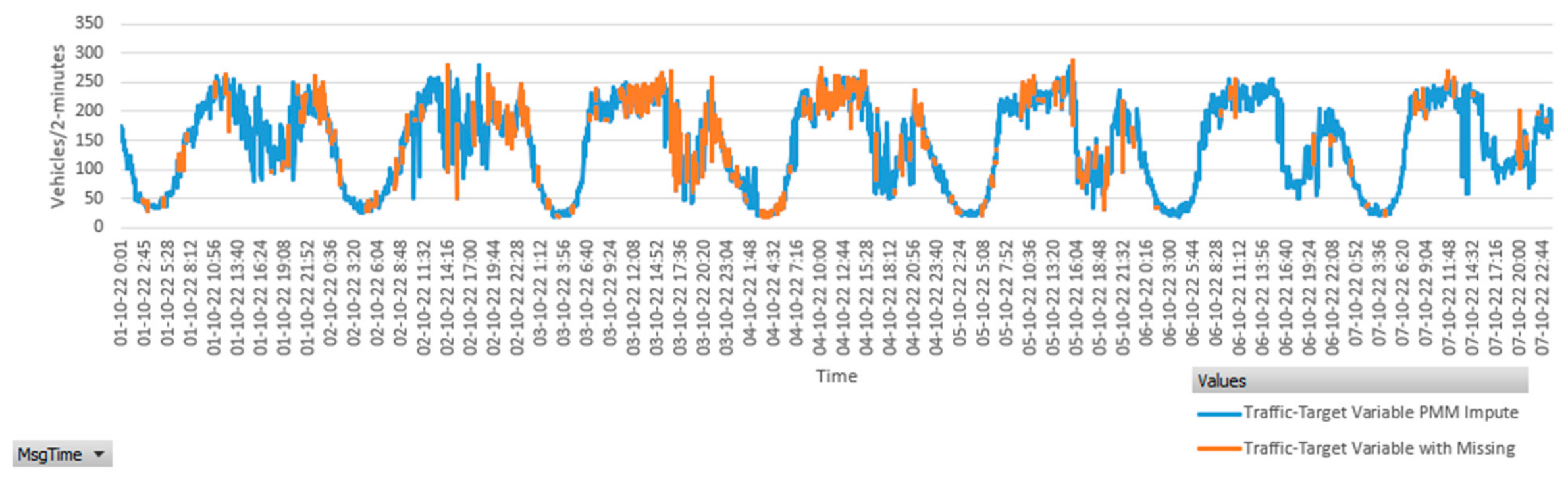
Figure 3 and Figure 4 show traffic volume across the first week of two sensors (low missing and high missing cases) as an example visualization of how gaps are sparse and how well the predictor line is fitted and smooth along the series.

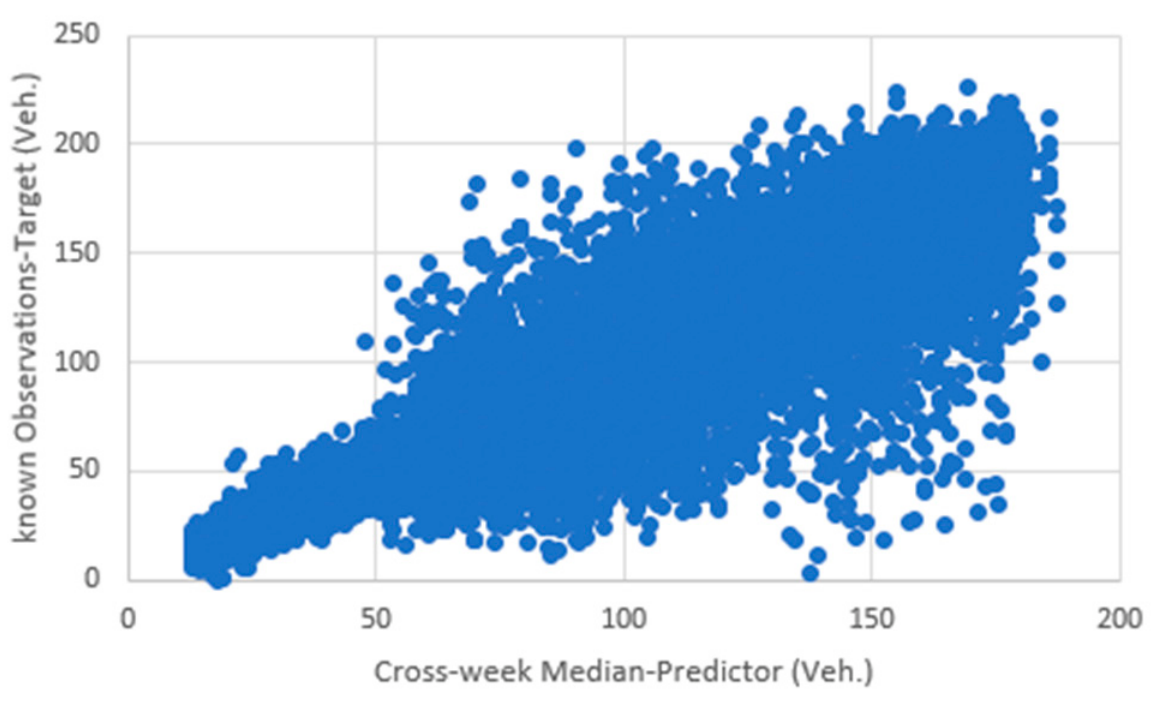
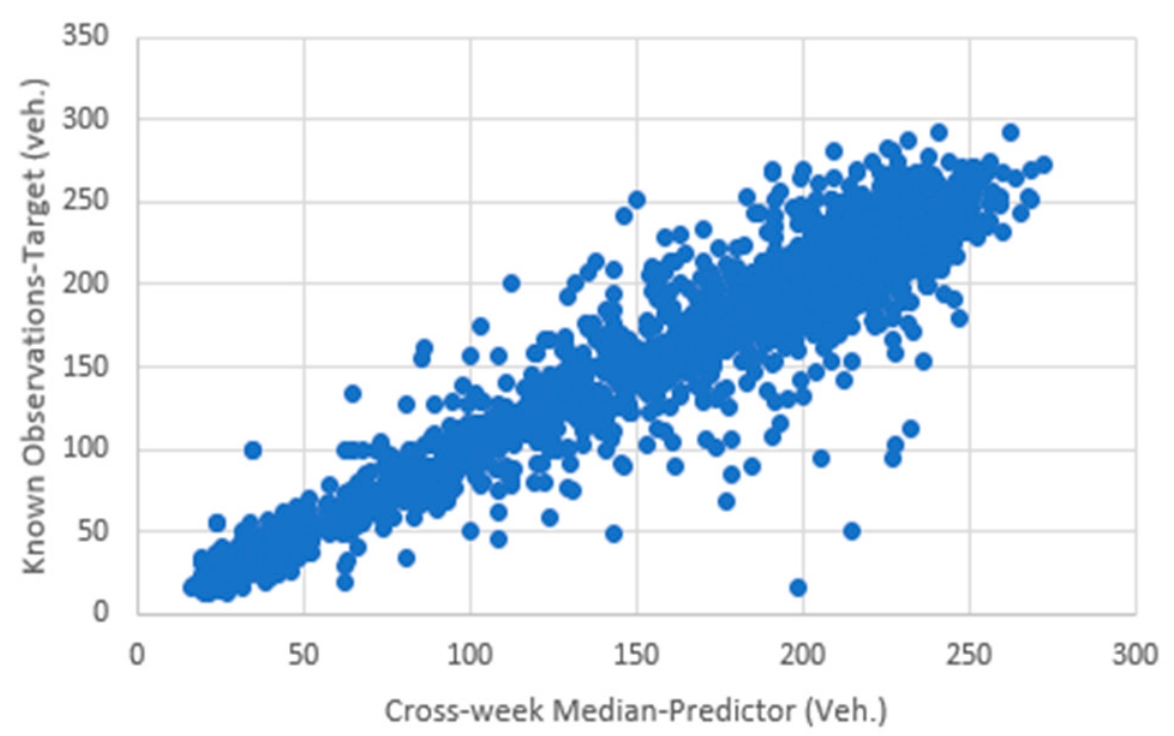
For the validation tests, the algorithm randomly selects 20% of the observed, non-missing traffic volume data for out-of-sample testing groups, where these vectors are masked to simulate artificial missingness. Meanwhile, an OLS objective function is used to fit the linear regression model to the remaining 80% training partition with the corresponding profile-aware predictors. As shown in Figure 5 and Figure 6, the linear regression framework successfully captures this underlying relationship. Statistical diagnostics on the 20% validation holdout (comprising 500 to 4150 observations) demonstrate an exceptionally strong relationship, yielding high correlation coefficients (r ranging from 0.93 to 0.96) and robust coefficients of determination (R² ranging from 0.86 to 0.92) between the cross-week median predictor and the dependent traffic volume variable. Moreover, Y-intercept (or regression constant) values were few, between 1 and 3 vehicles, which means there is no systemic bias or arbitrary scaling artifact in the engineered feature. The predictor is directly proportional to real physical traffic flow. The high accuracy and minor residual variance expressed by the linear regression engine are gained from the extreme similarity of traffic patterns at identical times of day across consecutive weeks. Because the dataset exhibits strong daily and weekly seasonality combined with rigorous short-term autocorrelation, the engineered profile-aware predictor operates as a highly stable proxy that reflects the true physical state of the highway traffic stream.

4.4. Dynamic Multiple Imputation

After fitting the linear regression model, the algorithm enters a dynamic imputation loop to estimate missing traffic volume values during each cycle. It utilizes the predictor dataset in the regression framework to generate three sets of estimates: first, values to fill in the originally missing data; second, temporary target values used to calculate neighborhood distances for PMM-ABB; and third, values to replace artificially masked data for cross-validation testing. During this step, a random Gaussian noise value is calculated and added to the deterministic predictions for the missing data points. Crucially, this noise component is updated independently with each iteration, preventing the artificial smoothing of the imputed traffic time series.

Within the iterative execution architecture, the framework evaluates the donor pool size from the candidate list by utilizing MAE and automatically adopts the optimal donor pool size (K) for the PMM-ABB engine. This optimization yields a diverse distribution of auto-adopted donor sizes across successive imputation cycles.

However, Figure 7, Figure 8, Figure 9 and Figure 10 demonstrate that the values generated by both imputation methods align seamlessly with the temporal structure of the traffic data. Visual inspection confirms the preservation of the temporal and physical continuity of the flow stream. Crucially, the framework did not generate negative volume estimates, while post-imputation diagnostics via the IQR method confirm that no artificial anomalies were introduced during the imputation process.

The engineered predictor has such an elite linear Pearson correlation (r = 0.93 to 0.96) to the target data that the parametric model uncertainty (the variation in the coefficients across bootstrap loops) is remarkably small, as shown in

Table 4. Comparison of Rubin’s Rule pooling variance.

Sensor ID	Regression-Based Imputation				PMM-Based Imputation
	Rubin-B	Rubin-U	Rubin-SE	Confidence Interval	Rubin-B	Rubin-U	Rubin-SE	Confidence Interval
R268	0.1827	1.1238	1.1453	106.4–110.9	0.6052	1.1277	1.3230	106.12–111.3
R2	0.3415	1.8004	1.4682	141.4–147.2	1.1804	1.9200	1.7682	141.1–148.1
R90	0.3596	3.2689	1.9252	143.7–151.2	0.7124	3.2699	2.0027	143.5–151.4
R417	0.2935	0.2766	0.7577	142.3–145.3	0.3182	0.2762	0.7739	142.3–145.4

. Because the regression line itself is so stable, the simulation reproducibility noise (MCE) drops instantly. However, the total standard error continued to drift, requiring more loops, as illustrated in

Table 5. Comparison of dynamic imputation convergence cycles.

Sensor ID	Regression-Based Imputation				PMM-Based Imputation
	Imputation Cycle When ∆SE < 1%	Imputation Cycle When MCR < 10%	SE When MCR Converge	MCE	Imputation Cycle When ∆SE < 1%	Imputation Cycle When MCR < 10%	SE When MCR Converge	MCE
R268	15	15	1.14	0.11	30	25	1.32	0.13
R2	20	15	1.45	0.32	50	45	1.72	0.16
R90	20	20	1.8	0.19	25	25	2.02	0.16
R417	50	55	0.76	0.064	55	60	0.79	0.078

. This is because the within-imputation variance represents the real, high-frequency, 2 min physical traffic randomness. It takes more loops for that real-world stochastic volatility to perfectly stabilize its cumulative average. For this reason, data randomness is driving the standard error stability, not model-parameter instability. However, because the hybrid predictor is so tightly bound to real physics, the residuals are microscopic. The stochastic noise added is so small that the model naturally preserves physical reality. Table 5 exhibits that the PMM-ABB framework requires systematically larger imputation cycles to achieve simultaneous convergence compared to the stochastic linear regression model. Conversely, PMM-ABB utilizes a stochastic drawing process through randomized selection from a discrete K-nearest neighbor donor pool; real-world donor pools inject additional simulation noise into the timeline or shifts in within-imputation variance, which drive the standard error stability as we observed. Consequently, the algorithm must execute more cycles to satisfy the rigorous threshold. Proving the precision of the dynamic stop bounds despite requiring more cycles, at convergence, the total standard errors remain small relative to the absolute scale of the daily highway volumes (ranging from a minimum of 0.76 at R417 to a maximum of 2.02 vehicles at R90). This demonstrates that the imputed values are tightly bounded around the localized temporal trends. Based on low values of the simulation error (MCE), they statistically guarantee high replicability. The results reveal dynamic variations in convergence bottlenecks across the network. For instance, at Sensor R417, achieving the Monte Carlo Ratio threshold required more cycles than stabilizing the standard error. Conversely, for Sensor R2, standard error stability required more cycles than the MCR target, while other instances (such as R268 and R90) converged simultaneously. The framework successfully prevents premature termination by forcing the algorithm to wait until both metrics are satisfied to guarantee that every sensor was imputed with optimal RE. The impact of the missing sequence volume for sensor R417 represents a unique operational anomaly within the corridor, requiring the highest number of simulation cycles across both methods. This prolonged convergence behavior is directly tied to its physical data profile, which contains massive, multi-day consecutive block dropouts (up to 3003 missing intervals). When a dataset experiences prolonged, continuous data voids, the within-imputation variance between consecutive missing blocks drops because the values are generated from the same long-term predictive trend line. However, the between-imputation variance across parallel runs expands dramatically because each independent bootstrap loop shifts the slope parameter. The FMI is extremely high at this particular location (see

Table 6. Comparison of efficiency parameters.

Sensor ID	Regression-Based Imputation			PMM-Based Imputation
	FMI	RE	PL	FMI	RE	PL
R268	0.138	0.991	0.009	0.351	0.99	0.010
R2	0.411	0.984	0.016	0.381	0.992	0.008
R90	0.192	0.99	0.010	0.179	0.993	0.007
R417	0.531	0.993	0.007	0.552	0.99	0.010

); for this reason, the overall standard error remains highly sensitive to parameter changes. The algorithm is forced to expand its execution matrix adaptively to 50–60 cycles to damp out this between-imputation volatility and satisfy the dual-criteria thresholds.

Across the corridor, R417 exhibits the highest FMI: 0.531 (regression) and 0.552 (PMM-ABB). This means that over 53% to 55% of the total uncertainty is driven by between-imputation variances. The RE values hover uniformly between 0.984 and 0.993. In MI theory, a value near 1.0 indicates that the number of imputation cycles executed by the dynamic stopping algorithm is more than sufficient to yield stable point estimates. This is further validated by the negligible PL metrics. With these values, there is no need to expand the simulation cycles further. Unlike historical implementations of MI that broadly recommend over 100 to 200 simulation cycles to suppress simulation noise, this framework achieves absolute convergence in a maximum of 60 loops (Sensor R417) and as few as 15 loops (Sensor R268). This extreme computational efficiency is directly attributable to the design of the hybrid, profile-aware historical median predictor.

Table 4 exhibits the basic structural differences between the regression imputation method and the PMM imputation frameworks through variance analysis. For both methods, the within-imputation variance heavily dominates the between-imputation variance. This structural imbalance indicates that the traffic flow variations within the individual daily and weekly time-series intervals are significantly higher than the differences between the parallel imputed datasets.

This shows that the cross-week historical median predictor works the same way in all parallel simulation runs. The historical traffic pattern is so accurate and steady that the model produces the exact same reliable results every time it runs; it tracks real, consistent human driving habits throughout the weeks.

The results of the between-imputation variance of PMM-ABB yield a noticeably higher value compared to stochastic regression. This increase is a direct consequence of PMM-ABB’s donor assignment stage. While the regression model draws smoothly from a continuous Gaussian distribution centered on the regression line, PMM-ABB randomly selects real, discrete vehicle values from a localized K-nearest neighbor donor pool. This discrete switching across different traffic days injects an expected variation premium into the parallel datasets, which slightly increases the standard error. It is the only R417 station where the between-imputation variance (B = 0.2935) exceeds its within-imputation variance (U = 0.2766) due to the massive missing sequence blackout. Sensor R417 data already had 88.9% of its data missing, while the known values are scattered randomly within the series. The model was trained on an extremely small portion of known values, and they were highly aligned with the seasonal baseline wave. Because the true micro-fluctuations are permanently lost during this massive blackout, the model output collapses onto a pure, clean seasonal pattern. This behavior represents a deterministic smoothing artifact of the historical baseline rather than an active reconstruction of real-time physical micro-variations. However, this stabilization is functionally necessary; it prevents matrix singularities within the OLS engine and provides the variance-protected macro-periodic profile required to maintain the stability of downstream continuous applications.

4.5. Multi-Domain Validation Results and Performance Synthesis

To assess how well the proposed imputation framework performs, we used four independent validation approaches: point estimation accuracy, continuous block tracking (temporal cross-validation), sequential time-dependency matching (ACF), and frequency-domain structural verification (spectral density).

4.5.1. Analysis of Random Holdout Validation Results

To rigorously map the predictive boundaries of the proposed MI frameworks, their point estimation accuracy was evaluated against a robust, highly competitive deterministic HA. The performance synthesis across Holdout-MAE, RMSE, and $R^2$ (

Table 7. Comparison of point estimation accuracy using Holdout-MAE.

Sensor ID	Regression-Based Imputation	PMM-Based Imputation	HA-Based Imputation
R268	22.233 ± 0.5	20.093 ± 0.61	17.27
R2	27.331 ± 0.55	24.49 ± 0.7	21.031
R90	27.746 ± 0.59	24.709 ± 0.64	21.422
R417	25.4 ± 1.41	23.6 ± 1.21	27.64

,

Table 8. Comparison of point estimation accuracy using Holdout-RMSE.

Sensor ID	Regression-Based Imputation	PMM-Based Imputation	HA-Based Imputation
R268	28.925 ± 0.68	28.575 ± 1.08	24.768
R2	35.45 ± 0.7	35.315 ± 1.34	30.909
R90	35.961 ± 0.67	35.387 ± 0.98	31.223
R417	35 ± 1.67	34.7 ± 1.93	40.068

and

Table 9. Comparison of point estimation accuracy using Holdout-R².

Sensor ID	Regression-Based Imputation	PMM-Based Imputation	HA-Based Imputation
R268	0.71679 ± 0.012	0.72354 ± 0.003	0.79
R2	0.77075 ± 0.009	0.77245 ± 0.017	0.82
R90	0.74894 ± 0.009	0.75686 ± 0.013	0.81
R417	0.799 ± 0.019	0.803 ± 0.021	0.74

), under stable telemetry or normal operational conditions (Sensors R268, R2, and R90), shows that the deterministic HA baseline yields numerically lower absolute and squared errors. Furthermore, the HA baseline produces a higher proportion of variance $R^2$. Localized averaging (especially the fallback to averaging neighboring intervals) inherently suppresses natural data variance, producing an artificially smoothed trajectory that mathematically minimizes residual metrics. This is in contrast to the proposed models, which preserve the micro-fluctuations of traffic by adding Gaussian noise or randomly drawing nearest neighbors. Preserving this variance is mathematically critical for high-frequency continuous data required to feed downstream ITS applications such as DTA, as artificially smoothed data prevents downstream models from accurately simulating vehicle speed reduction, bottleneck formations, and high-variance shock wave mechanics. Stochastic regression imputation introduced a higher absolute error than the PMM method; the stochastic part, represented by the constant Gaussian noise (residual noise) added to the predicted values, causes fractional variations, resulting in cumulative point-to-point misalignments across thousands of 2 min intervals. This could be the reason behind the marginally higher absolute error, while the PMM uses deterministic regression as a metric to draw real values from historical adjacent intervals that match the exact traffic state, close to the actual observed data. In the case of testing validation on a random 20% holdout, it reveals the superiority of the PMM imputation method over the regression imputation method. Nonetheless, the calculated Cohen’s d value showed no practical difference in point estimation accuracy for the standardized difference of the absolute residuals of the two stochastic models, and the result was approximately zero.

Cohen’s d was calculated to measure the effect size of absolute residuals between the proposed methods and the HA baseline (

Table 10. Cohen’s d values comparing point estimation absolute residuals of the models to the HA method.

Proposed Models	R268	R2	R90	R417
Regression-Based Imputation	0.3	0.3	0.2	−0.1
PMM-Based Imputation	0.1	0.1	0.1	−0.1

). For sensors R268, R2, and R90, the Cohen’s d values range tightly between 0.1 and 0.3; this represents a small to negligible effect size and confirms that while the Stochastic Regression and PMM-ABB frameworks successfully inject the necessary physical noise into the imputed time series, the standardized magnitude of their point-error deviation from a highly optimized deterministic HA baseline is practically marginal.

The fundamental limitation of the localized deterministic HA baseline method is exposed under severe telemetry failure. At Sensor R417, which exhibits a massive, continuous multi-day block, the HA algorithm rapidly exhausts its primary historical matches (the same day of the week and exact time slot and the localized 14 min past-neighboring fallback) due to consecutive data drops. The HA algorithm is forced to trigger its ultimate fail-safe: imputing the global arithmetic average. Imputing a flat global mean across long blocks of voids destroys the physical variance or the micro-fluctuations of the traffic flow. Consequently, the HA baseline’s performance degrades significantly, with MAE climbing to 27, RMSE expanding to 40, and R² dropping to 0.74. In contrast, the proposed frameworks (Stochastic Regression and PMM-ABB) demonstrate rigorous systemic resilience when handling Sensor R417. Crucially, they survive this high data loss because they do not rely on the preceding 14 min as their primary or ultimate fail-safe (imputing the global average). Instead, their survivability is driven by the hybrid, multi-tier adaptive predictor. Rather than abruptly collapsing to a global median, the predictor automatically widens its localized cross-week window (expanding from ±6 min up to ±30 min) to locate valid historical medians, values closer to the missing point than the global average. Thus, the proposed models successfully minimize reliance on flat global averages. This adaptive scaling preserves localized temporal structures, restricting MAE to ~23.6 to 25.4, RMSE to ~34.7 to 35, and maintaining an R² of ~0.80. The Cohen’s d matrix (Table 10) provides definitive statistical confirmation of this superiority. Under prolonged missing data stress, the standardized effect sizes invert to negative values (−0.1 for both Regression-Based and PMM-Based Imputation). This negative shift indicates that the proposed stochastic models systematically reduce absolute residual errors compared to the HA baseline.

Under normal operational conditions with sparse missingness (Sensors R268, R2, R90), the framework successfully preserves natural traffic variance. However, a distinct smoothing artifact occurs under the extreme data starvation observed at Sensor R417. Because the algorithm rarely finds multiple historical cross-week data points for the same time interval during these massive multi-day blackouts, localized micro-fluctuations are severely suppressed. The interacting factors of prolonged consecutive gaps and the stationarity of the time series force the output to collapse onto a pure macro-seasonal wave.

While this mathematical smoothing artifact masks the true high-frequency stochastic micro-fluctuations of the traffic flow, it crucially prevents the severe error inflation observed in the HA baseline. Therefore, the performance metrics at R417 should not be interpreted as the framework perfectly capturing localized micro-variance. Instead, the true advantage of the framework at this location is its systemic survivability. By utilizing the adaptive structural anchor, the MI engine successfully reconstructs the temporal block without the computational crashes and exploding residual errors inherent to traditional deterministic baselines.

Sensor R268, on the other hand, recorded lower traffic flow values than the intense traffic flow values recorded by other stations. Records from other sensors show that 19 to 21% of their traffic data exceed the traffic flow capacity recorded by Sensor R268. The traffic volume metrics are absolute scales, which means segments with a lower flow capacity produce smaller absolute residuals. Consequently, validation methods basically utilize absolute/square residuals, such as point accuracy (Table 7, Table 8 and Table 9) and cross-validation (the first and second tables in Section 4.5.3), which revealed low error values for the segment where Sensor R268 is located. It is critical to formally distinguish between the engineered cross-week median (which serves strictly as the independent input predictor feature) and the validation benchmark (which consists exclusively of the true, unmasked RTMS field observations). The evaluation metrics strictly measure the distance between the model’s final stochastic output and the physical field data, not how well the model replicates its own input feature.

A critical dimension of the multi-domain validation is the statistical reproducibility of the MI engine, which is quantified by the non-parametric percentile 95% bootstrap confidence intervals. Across all monitoring stations, both the Stochastic Regression and PMM-ABB frameworks exhibit highly constrained empirical confidence margins. As shown in Table 7, Table 8 and Table 9, the variance remains remarkably tight relative to the overall error magnitudes, with Holdout-MAE strictly bounded between ±0.5 and ±1.41 vehicles, Holdout-RMSE between ±0.67 and ±1.93 vehicles, and R² variance limited to a maximum of ±0.021. Because these intervals map the true, unshrunk empirical variance across all imputation cycles, their stability provides definitive proof that the dual-metric dynamic stopping algorithm functioned exactly as intended. By adaptively extending the imputation cycles ($M$) until Rubin’s Standard Error stabilized and the MCE dropped below the 10% threshold, the framework successfully damped out initial simulation-induced volatility. Consequently, the reported metrics are not artifacts of a single stochastic draw or erratic simulation noise, but represent a highly stable, reproducible convergence that accurately captures the physical variance of the network.

4.5.2. Analysis of the Autocorrelation Validation Results

The performance inversion observed in the point-estimation holdout method—where deterministic smoothing artificially minimized localized absolute residuals on stable sensors—necessitates a rigorous evaluation of the chronological structure of the imputed data. While point-estimation methods strictly measure localized accuracy, ACF at lag $h=720$ (24 h) is utilized to verify the preservation of daily traffic patterns, sequential time-dependencies, and physical memory. The results in

Table 11. Comparison among models utilizing autocorrelation validation MAE.

Sensor ID	Regression-Based Imputation	PMM-Based Imputation	HA-Based Imputation
R268	0.0018 ± 0.0005	0.0017 ± 0.0007	0.0022254
R2	0.0018 ± 0.0008	0.0016 ± 0.0006	0.0025227
R90	0.0026 ± 0.0009	0.0019 ± 0.0012	0.0046112
R417	0.0007 ± 9 × 10 −5	0.0008 ± 0.0001	0.0013692

,

Table 12. Comparison among models utilizing autocorrelation validation RMSE.

Sensor ID	Regression-Based Imputation	PMM-Based Imputation	HA-Based Imputation
R268	0.0024 ± 0.0005	0.0023 ± 0.0007	0.0029708
R2	0.0022 ± 0.0008	0.002 ± 0.0007	0.0030134
R90	0.0030 ± 0.001	0.0023 ± 0.0013	0.0051061
R417	0.0009 ± 0.0001	0.001 ± 0.0002	0.001676

and

Table 13. Cohen’s d values compare ACF absolute residuals of models to the baseline method.

Proposed Models	R268	R2	R90	R417
Regression-Based Imputation	−0.2	−0.5	−1.2	−0.9
PMM-Based Imputation	−0.3	−0.6	−1.8	−0.8

resolve the smoothing paradox by exposing the structural cost of deterministic averaging. Across all four monitoring stations, the HA baseline uniformly records the highest temporal structural errors, exhibiting peak ACF-MAE and ACF-RMSE values (e.g., 0.0025 at R2). This across-the-board degradation occurs because deterministic averaging strips away sequential chronological memory. While averaging same-day/same-time past intervals produce a flat trajectory that scores well on point-by-point holdout tests for stable sensors, it completely annihilates the natural, auto-correlated micro-fluctuations (the physical inertia of traffic flow moving from one 2 min interval to the next). Conversely, as shown in Table 11 and Table 12, both proposed imputation methods showed extremely low autocorrelation errors across all four sensors. This indicates that the imputed missing sequences successfully recreate the native daily traffic waves. By rejecting artificial smoothing, these frameworks successfully reconstruct the native cyclic rhythms of the highway. Notably, PMM-ABB consistently edges out Stochastic Regression in preserving autocorrelation (e.g., an ACF-MAE of 0.0016 vs. 0.0018 at Sensor R2, and 0.0019 vs. 0.0026 at R90). This nuanced superiority refers to the selected donor in the PMM-ABB framework being a real, highly correlated temporal neighbor to the masked value; this localized state-matching is repeated efficiently whenever the imputation operates. For this reason, the autocorrelation metric results of PMM were closely aligned with, yet slightly superior to, the regression method results. Ultimately, both proved the immense power of the engineered predictor within the sophisticated imputation framework in preserving the daily traffic pattern.

The Cohen’s d matrix (Table 13) provides powerful statistical validation of this structural superiority, directly contrasting with the holdout point-accuracy findings. In the previous holdout analysis, the standardized effect size between the models and the baseline on stable sensors was negligible ($d\le 0.3$). However, when evaluating the absolute residuals of the temporal structure, the effect sizes invert to heavily negative values across the entire network. For Sensor R90, the PMM-ABB framework achieves a massive structural effect size of −1.8, and a −1.2 for Stochastic Regression. At Sensor R417, which suffered from severe data loss, the models maintain large negative effect sizes (−0.9 and −0.8). These magnitudes definitively prove that the proposed stochastic models systematically and substantially reduce sequential dependency errors compared to the deterministic baseline. However, the calculated Cohen’s d value showed no practical difference in autocorrelation absolute error between the two stochastic models.

The reliability of these temporal reconstructions is empirically verified by the extremely tight non-parametric percentile bootstrap confidence intervals reported in Table 11 and Table 12. By evaluating the true empirical variance across all imputation cycles, the margins of error for the proposed models remain microscopic, strictly bounded between ±0.0013 and ±9 × 10 ⁻⁵. Even without artificial standard error shrinkage, these highly constrained limits prove that structural preservation is not the result of a single, favorable stochastic randomization. Instead, it confirms that the dual-metric dynamic stopping algorithm effectively damped out Monte Carlo simulation-induced volatility, allowing the non-parametric bootstrap resampling to precisely converge the macro-periodic autocorrelations of the traffic network, stabilizing the baseline regardless of the severity of the telemetry failure. Both stochastic models proved the immense utility of the engineered predictor in preserving the essential daily traffic patterns without mathematical collapse.

4.5.3. Analysis of Temporal Cross-Validation

The temporal cross-validation metrics provide a rigorous evaluation of how well the imputation frameworks reconstruct missing data blocks across unknown time periods. By calculating validation metrics on a completely hidden continuous week, this method serves as a confident test of structural predictive accuracy under real-world sensor failure conditions. This directly contrasts with the random holdout method, where the masked validation data is sparse and randomly scattered over the 31-day horizon. This validation forces the imputation engines to reconstruct extended temporal voids without the aid of immediate, adjacent-interval neighbors. The results from the T-CV-MAE (

Table 14. Comparison among models utilizing T-CV-MAE.

Sensor ID	Regression-Based Imputation	PMM-Based Imputation	HA-Based Imputation
R268	16.855 ± 0.015	15.997± 0.024	16.856
R2	19.758 ± 0.018	19.756 ± 0.024	19.776
R90	19.638 + 0.018	19.634 + 0.03	19.628
R417	22.761 + 0.066	22.777 + 0.077	33.778

), T-CV-RMSE (

Table 15. Comparison among models utilizing T-CV-RMSE.

Sensor ID	Regression-Based Imputation	PMM-Based Imputation	HA-Based Imputation
R268	23.216 ± 0.005	23.212 ± 0.012	23.214
R2	27.844 ± 0.007	27.842 ± 0.011	27.845
R90	27.975 + 0.008	27.98 + 0.009	27.98
R417	33.965 + 0.054	33.977 + 0.073	41.52

), and the standardized effect sizes (

Table 16. Cohen’s d values compare temporal-CV absolute residuals of models to the baseline method.

Proposed Models	R268	R2	R90	R417
Regression-Based Imputation	0.1	0.1	0.0	−0.4
PMM-Based Imputation	0.1	0.1	0.0	−0.4

) expose the true structural robustness of the methodologies under prolonged operational stress.

In the temporal cross-validation method, masking an entire continuous weekly block forces the models to train using data exclusively from other weeks. This chronological isolation slightly shifts the baseline regression parameters. More critically, it fundamentally impacts the PMM-ABB donor selection process. Because the target week is hidden, the framework is forced to draw discrete donor vehicle counts from noncontiguous intervals located in adjacent weeks, rather than from the same day or a closely neighboring day. Under the continuous block mask, the deterministic HA algorithm is stripped of its ability to use its immediate 14-min local fallback, forcing it to rely exclusively on cross-week historical matches. Because the proposed stochastic models also derive their primary structural anchor from the engineered cross-week median predictor, the performance of all three methods converges tightly. For sensors R2 and R90, the MAE and RMSE values are virtually indistinguishable. However, at Sensor R268, PMM-ABB demonstrated a distinct advantage, achieving an MAE of 15.997 compared to 16.855 for both Regression and the HA baseline. The general convergence across stable sensors is verified by the Cohen’s $d$ matrix (Table 16). The standardized effect sizes for these three sensors drop to exactly 0.0 or 0.1. This statistical equivalence proves that when forced to reconstruct massive blocks using historical data, the proposed frameworks deliver baseline accuracy competitive with a highly tuned deterministic model while simultaneously preserving the physical wave structures required for ITS applications (i.e., DTA). Results of the Cohen’s d test showed no practical difference in temporal cross-validation absolute error between the two stochastic models.

The profound superiority of the proposed imputation architecture is exposed at R417, which already suffers from massive, continuous hardware blackouts in the training data. When the T-CV algorithm artificially masks an additional week for validation, the historical data pool is entirely wiped out. Under this extreme historical starvation, the HA baseline completely collapses. Unable to find cross-week matches and lacking any immediate local neighbors, it falls back to the global arithmetic mean for the entire week. Consequently, the HA error metrics exploded, with T-CV-MAE reaching 33.778 and T-CV-RMSE hitting 41.52. Conversely, the Stochastic Regression and PMM-ABB models demonstrate exceptional survivability. Their multi-tier adaptive predictor has an automatic widening search window (expanding up to ±30 min) to locate valid, highly correlated historical medians. By dynamically scaling these proxies via optimized regression coefficients, the proposed models completely avoid the global average trap. They maintain exceptional structural accuracy, suppressing the T-CV-MAE to ~22.77 and the T-CV-RMSE to ~33.97. The Cohen’s $d$ results for Sensor R417 (Table 16) quantify this systemic rescue. With an effect size of −0.4 for both Stochastic Regression and PMM-ABB, the models achieve a moderate but structurally critical reduction in absolute residuals compared to the baseline’s severe failure.

Finally, the integrity of these cross-validation reconstructions is cemented by the non-parametric percentile bootstrap confidence intervals (Table 14 and Table 15). By evaluating the true empirical variance across the MI loops, the generated margins of error remain exceptionally tight, ranging strictly between ±0.005 and ±0.077 vehicles. Relative to the overall magnitude of the validation errors, this highly constrained variance confirms that the dynamic stopping boundaries successfully dampen out simulation-induced volatility without erratic divergence. The algorithms achieved mathematically stable convergence across all iterative loops, proving that the framework is highly reproducible and resilient against extreme continuous data loss.

4.5.4. Frequency-Domain Macro Structural Preservation

While time-domain validations assess localized tracking and sequential dependencies, they do not fully capture the macroscopic wave harmonics and high-frequency white noise inherent in continuous traffic flow. To verify that the imputation frameworks preserve these large-scale traffic cycles (such as the distinct morning and evening peak commuter waves), the completed timelines were transformed from the time domain into the frequency domain through a periodogram using FFT to estimate the PSD. The results across

Table 17. Comparison among models utilizing similarity-normalized spectral density.

Sensor ID	Regression-Based Imputation	PMM-Based Imputation	HA-Based Imputation
R268	0.31639 ± 0.1	0.31744 ± 0.12	0.39268
R2	0.33697 ± 0.099	0.30823 ± 0.084	0.33768
R90	0.40167 ± 0.01	0.35966 ± 0.012	0.41853
R417	0.11445 ± 0.013	0.11794 ± 0.014	0.19367

,

Table 18. Comparison among models utilizing spectral density MAE (log-scale dB).

Sensor ID	Regression-Based Imputation	PMM-Based Imputation	HA-Based Imputation
R268	3.319 ± 0.075	3.29 ± 0.093	3.0057
R2	2.71 ± 0.05	2.7 ± 0.09	2.4248
R90	3.13 ± 0.063	3.09 ± 0.073	2.819
R417	0.8 ± 0.05	0.817 ± 0.073	1.7052

and

Table 19. Comparison among models utilizing spectral density RMSE (log-scale dB).

Sensor ID	Regression-Based Imputation	PMM-Based Imputation	HA-Based Imputation
R268	4.81 ± 0.09	4.79 ± 0.13	4.4832
R2	4.05 ± 0.093	4.03 ± 0.118	3.6895
R90	4.58 ± 0.096	4.54 ± 0.12	4.1992
R417	1.46 ± 0.088	1.47 ± 0.122	1.8388

definitively demonstrate that the proposed stochastic models preserve the true structural energy of the traffic stream, overriding the superficial benefits of deterministic baseline smoothing.

By implementing a logarithmic decibel scale (dB) for error tracking, the validation reveals that the spectral values for the proposed models remained within stable bounds, with an upper limit in MAE of 3.32 dB and 4.81 dB for RMSE across all operational sensors. This proves that the reconstructed time series very well reproduces the spectral energy distribution and the periodic harmonic profile of the original dataset. This preservation is further highlighted by the Similarity-Normalized Spectral Density (Table 17). Across the monitoring stations, both Stochastic Regression and PMM-ABB systematically outperform the deterministic HA baseline. While the deterministic HA algorithm severely distorts the overall energy profile by artificially flattening the data, the stochastic frameworks successfully preserve high-frequency variance during sparse dropouts and secure the fundamental macro-wave periodicities that define daily human commuting cycles during extreme block-missingness.

A prominent finding from the spectral analysis is the near-identical performance between the regression-based imputation and the PMM-ABB based framework across all four monitoring stations. Both frameworks successfully reconstruct the underlying cyclic rhythms and characteristic energy patterns. However, PMM-ABB reveals a slightly higher performance profile. This nuanced superiority occurs because PMM-ABB leverages the deterministic regression line strictly as a matching metric to draw discrete, real vehicle counts from immediate temporal neighbors that match the exact traffic state. This non-parametric approach allows PMM to perfectly preserve the natural, stochastic fluctuations of the data. On the other hand, the fixed Gaussian noise added to the regression estimates can cause individual imputed points to diverge slightly from the actual observations, resulting in a minor deviation in the physical signal’s frequency phase.

A unique phenomenon emerges at Sensor R417, which actually achieves the highest spectral matching scores (the lowest absolute dB errors, such as a PSD MAE of 0.8 dB for Regression and 0.817 dB for PMM) in this study. This counterintuitive performance spike is directly due to the nature of its extensive, consecutive gaps, which isolate the evaluation from high-frequency, minute-by-minute stochastic fluctuations; the imputation framework naturally bypasses localized daily noise. Instead, it successfully reconstructs a stable, macro-periodic signal wave that aligns cleanly with the true structural energy profile of the network. In contrast, the HA baseline completely fails under these exact same massive dropouts; its reliance on a flat global arithmetic average destroys the harmonic profile, resulting in a significantly worse PSD MAE of 1.7052 dB. The integrity of these frequency-domain reconstructions is empirically validated by the non-parametric percentile bootstrap confidence intervals (Table 17, Table 18 and Table 19). By mapping the true empirical variance across the MI loops, the 95% confidence margins reflect highly realistic and stable uncertainty bounds (e.g., PSD MAE margins tightly constrained between ±0.05 and ±0.093 dB, and Spectral Similarity margins bound between ±0.01 and ±0.12). These bounded, data-driven intervals verify that the stochastic models successfully capture the natural structural fluctuations of the traffic network, and that the macro-periodic wave generation remains mathematically reproducible without erratic divergence.

To contextualize the raw logarithmic decibel errors and objectively measure the performance differences,

Table 20. Cohen’s d values of PSD absolute residuals of models compared to the HA baseline method.

Proposed Models	R268	R2	R90	R417
Regression-Based Imputation	0.1	0.1	0.1	−0.2
PMM-Based Imputation	0.0	0.1	0.0	−0.2

presents the Cohen’s $d$ values comparing the absolute spectral residuals of the proposed models against the HA baseline. For the stable sensors operating under sparse missingness (R268, R2, and R90), the standardized effect sizes are negligible, ranging strictly from 0.0 to 0.1. This provides critical statistical confirmation of the frameworks’ efficiency. It proves that while the proposed models successfully inject the stochastic variance necessary to preserve high-frequency physical realism, this variance does not cause any statistically meaningful degradation in spectral accuracy compared to the heavily smoothed deterministic baseline. However, the calculated Cohen’s d value shows no practical difference in spectral density absolute error between the two stochastic models.

Furthermore, the true systemic advantage of the proposed frameworks is quantified at Sensor R417. Under the stress of continuous, multi-day block dropouts, the Cohen’s $d$ values invert to −0.2 for both Stochastic Regression and PMM-ABB. This negative shift definitively proves that the models’ ability to bypass localized noise and anchor to uncorrupted macro-periodic waves delivers a statistically significant reduction in spectral error compared to the baseline’s catastrophic reliance on a flat global average. Ultimately, the close alignment and stable spectral performance between both stochastic imputation methods indicate that the engineered profile-aware historical median predictor functions as an exceptionally robust structural foundation for traffic state reconstruction.

5. Conclusions

This study developed and rigorously evaluated a robust, profile-aware MI framework designed to reconstruct missing traffic volume data from RTMS (RTMS). By integrating a parametric Stochastic Regression model with a non-parametric PMM-ABB engine—both powered by an adaptive feature-engineering pipeline—this research overcomes the traditional limitations of static, deterministic, and single-imputation methods. Through rigorous pre-modeling diagnostics and a comprehensive four-tier multi-domain validation process (Holdout, Temporal Cross-Validation, Autocorrelation, and PSD), the empirical results yield the following main conclusions:

• Telemetry Profiling and Data-Driven Diagnostics: Non-parametric Kolmogorov–Smirnov tests and generalized linear models rejected the MCAR hypothesis, proving that missingness is heavily structured by daily and calendar cycles (MAR). Boundary t-tests and extreme-value filtering confirmed that these data drops represent infrastructure-driven hardware blackouts rather than traffic-state anomalies (like congestion stalling). Furthermore, pre-modeling diagnostics classified the underlying sensor data as stationary processes (eliminating the risk of statistical drift) and identified an optimal autoregressive physical memory span of 20 min (10 lags).
• Convergence Mechanics and Variance Decomposition: Applying Rubin’s pooling rules provided fundamental insights into the variance structures of high-resolution traffic telemetry. For stable sensor segments, within-imputation variance heavily dominated between-imputation variance. However, under massive block drops (Sensor R417), between-imputation variance exceeded within-imputation variance. This proves that while massive dropouts smooth out local internal volatility, they amplify parameter estimation uncertainty across parallel runs—mathematically demonstrating why single-imputation methods are fundamentally invalid for extensive data repair. Additionally, the dual-criterion stopping rule (monitoring Rubin’s standard error and White’s Monte Carlo error ratios) successfully prevented premature termination, revealing that PMM-ABB requires higher computational cycles than Stochastic Regression due to the variance premium introduced by drawing from discrete real-world donor pools.
• The Fallacy of Deterministic Smoothing and Systemic Resilience: Under stable conditions with sparse missingness, the deterministic HA baseline obtained marginally lower point-estimation residuals. However, this study exposes this as a mathematical “smoothing paradox.” The HA algorithm inherently suppresses natural data variance, producing an artificially flattened trajectory. While this minimizes residual metrics, it completely annihilates the natural auto-correlated micro-fluctuations (physical inertia) required to reliably feed advanced downstream ITS applications. Furthermore, the HA baseline suffered severe degradation under catastrophic telemetry failure (Sensor R417), exhausting its historical matches and collapsing to a global arithmetic mean (Temporal-CV MAE exploding to 33.778 and RMSE to 41.52). In stark contrast, the proposed stochastic frameworks demonstrated rigorous survivability; by utilizing a multi-tier adaptive predictor that automatically widens its cross-week window (up to ±30 min), the models bypassed the global average trap, restricting T-CV MAE to approximately 22.77 and maintaining an R² of 0.80.
• Robust Performance Across Validation Architectures: A key methodological takeaway of this research is that PMM consistently outperforms Stochastic Regression across most evaluation metrics, regardless of the validation scheme applied. Under a random holdout setup, PMM maintains a slight performance advantage in minimizing absolute error because it directly incorporates observed, discrete traffic counts from adjacent-day data points.
• Superiority in Structural and Frequency-Domain Preservation: The proposed stochastic frameworks mathematically outperformed the HA baseline in preserving both sequential dependencies and macroscopic wave harmonics. PMM-ABB demonstrated distinct superiority in temporal integrity (achieving a massive structural Cohen’s d effect size of −1.8 at Sensor R90) because it draws real, highly correlated discrete vehicle counts from temporal neighbors. In the frequency domain, decibel-scaled (PSD) matching proved that both frameworks accurately mirror macro-level human periodicity (the 24-h traffic wave). The models retained the true spectral energy distribution of human driving behavior, keeping maximum spectral MAE strictly under 3.32 dB and overall spectral tracking errors bound below 4.81 dB.
• Robustness of the Profile-Aware Feature Foundation: Across all structural, temporal, and frequency-domain tests, both imputation models aligned seamlessly. This close convergence, combined with strict adherence to physical boundaries (zero negative estimates) and outlier-free outputs verified by the IQR method, confirms that the underlying multi-tier historical median predictor provides an exceptionally stable structural foundation, capable of preserving localized traffic dynamics under normal conditions and preventing mathematical matrix collapse during severe hardware failures.

6. Recommendations

Based on the empirical evidence and performance synthesis derived from this study, the following recommendations are proposed for ITS practitioners and future researchers:

• Mandate Multi-Domain Validation Protocols: Traffic engineering studies must cease relying solely on single point-estimation metrics (e.g., MAE, RMSE, and R²) or simple random holdout schemes to evaluate imputation models. As demonstrated by the smoothing paradox, these metrics falsely reward models that destroy physical variance. Validation loops must incorporate a dual-pronged framework consisting of random masking (to test localized behavior) and continuous block masking (to simulate real-world dropouts). Furthermore, autocorrelation (ACF) and PSD validations should be adopted as mandatory standards to guarantee that reconstructed signals match the native periodic energy and cyclic rhythms of human commuting behavior.
• Deploy Predictive Mean Matching with Approximate Bayesian Bootstrap for High-Frequency Microsimulation: For networks experiencing standard, sparse data loss, the PMM-ABB framework is highly recommended. Its non-parametric approach of drawing real, discrete historical vehicle counts from adjacent intervals perfectly preserves the natural, high-frequency stochastic fluctuations of the traffic stream without artificial smoothing. This makes it the superior choice for downstream applications requiring micro-level precision, such as DTA, shockwave simulation, traffic signal optimization, and environmental emission modeling.
• Deploy Stochastic Frameworks for Macro-Level Block Reconstructions: When entire continuous weekly blocks are missing or when conducting macro-planning and long-term trend analysis, both the Stochastic Regression and PMM -ABB frameworks are highly recommended over deterministic baselines. As demonstrated in the Temporal Cross-Validation results, both models successfully prevented the catastrophic collapse seen in the HA algorithm during multi-day hardware blackouts. While the Stochastic Regression engine stabilizes parameter variances through continuous Gaussian noise, PMM-ABB proved equally resilient—even marginally outperforming the baseline at specific stable sensors despite being forced to draw donors from noncontiguous, cross-week intervals. Consequently, practitioners can confidently deploy either of the proposed stochastic architectures to secure a robust, variance-protected data foundation for extended continuous blackouts.
• Implement Adaptive Windowing over Global Averaging: Traffic management centers must abandon legacy imputation systems with standard fixed-parameter imputation algorithms (such as classical SARIMA or Holt–Winters), which fail when encountering multi-day data voids or systems that default to global arithmetic averages during prolonged hardware blackouts. Systems should be upgraded to utilize hybrid, multi-tier adaptive predictors. By automatically widening the historical search window in the event of prolonged disconnects, this architecture locates correlated cross-week medians, thereby providing a stable, variance-protected data foundation without losing high-frequency resolution.
• Implement Dynamic Stopping Criteria: To optimize computational efficiency without sacrificing statistical replicability, MI engines should not depend on static, arbitrary iteration limits (e.g., blindly running 100+ loops). Instead, imputation systems must implement a dual-metric dynamic stopping algorithm that forces execution to continue only until both the localized cumulative standard-error stability threshold (e.g., 1%) and the MCE ratio (<10%) are met simultaneously.
• Reframe Historical Data as an Exogenous Feature Foundation: Future researchers should shift from using historical traffic profiles as direct data patches to utilizing them as an optimization guide (exogenous feature matrix) within a stochastic loop. This conceptual shift allows the framework to exploit long-term human commuting periodicity to stabilize parameter distributions and maximize computational convergence speed (achieving stability in as few as 15 to 60 loops), while completely evading the artificial smoothing artifacts inherent to traditional direct-fill baseline models.

7. Future Research and Implementation Recommendations

Based on the methodology developed and the statistical insight obtained in this study, the following lines of research are recommended for future academic research and industrial implementation:

• Extension to multimodal spatial networks: In future expansions, the feature space of the adaptive predictor should be adapted to include spatial telemetry relations (upstream and downstream donor sensors) in addition to the temporal cross-week links. This spatio-temporal integration will serve as a second line of defense should multiple contiguous sensors suffer network-wide telemetry blackouts simultaneously.
• Real-Time Edge Deployment: Explore computational optimizations to convert the dynamic loop MI framework into a near real-time data cleaning script that can run directly on edge-computing traffic management hardware, allowing for instant sensor self-repair.