Efficient Polish-Language Keyword Spotting on Microcontrollers: Compact Neural Architectures, Quantization, and On-Device Validation on the Raspberry Pi Pico 2

Abstract

Keyword spotting (KWS) is the always-on front end of voice interfaces; running it directly on microcontrollers, rather than streaming audio to the cloud, is essential for low-latency, privacy-preserving, and energy-efficient operation, yet it must reconcile high accuracy with severe memory, compute, and energy limits. Existing small-footprint KWS solutions are developed and benchmarked almost exclusively on English and are seldom validated on physical hardware or under quantization for other languages; their transferability to typologically different, consonant-rich languages such as Polish therefore remains largely unverified. We present a KWS pipeline for Polish, deployed and benchmarked on the RP2350 microcontroller (Raspberry Pi Pico 2, Raspberry Pi Ltd., Cambridge, Great Britain).We propose three compact architectures from the convolutional (CNN), convolutional recurrent (CRNN), and depthwise separable neural network (DS-CNN) families and benchmark them against the state-of-the-art BC-ResNet on a 25-keyword Polish vocabulary using MFCC features. All models are evaluated in full precision (Float32) and after eight-bit integer (INT8) post-training quantization, with inference latency measured directly on the target hardware. BC-ResNet attains the highest full-precision accuracy (97.81%) but is the most fragile under quantization, whereas the proposed CRNN is the most accurate quantized model (94.28%), the DS-CNN the smallest (46.15 KB), and the CNN the fastest (107.5 ms); all quantized models meet a one-second real-time budget. We further show that the accuracy ranking inverts after quantization, that memory savings are highly architecture-dependent, and that phonetically similar Polish words are the dominant source of error. These results offer practical guidance for deploying small-footprint KWS in Polish and other underrepresented languages.

1. Introduction

Voice interfaces have become one of the most natural and ergonomic methods of human–machine interaction. Keyword Spotting (KWS) is the task of detecting predefined words or short phrases in a continuous audio stream. It constitutes the foundation of modern virtual assistants, such as Amazon Alexa, Apple Siri, and Google Assistant, where a lightweight, always-on detector listens for a wake word before activating more complex processing pipelines.

With the rapid expansion of the Internet of Things (IoT), there is a growing demand for touchless operation of smart-home appliances and industrial automation systems. However, streaming audio to remote cloud servers introduces critical challenges, including unacceptable latency, high network bandwidth usage, increased power consumption, and privacy concerns regarding user data [1]. A remedy is offered by Edge Computing and the TinyML paradigm, which shift acoustic analysis directly onto low-cost microcontrollers at the edge of the network.

Historically, speech recognition was dominated by Hidden Markov Models (HMMs) combined with Gaussian Mixture Models (GMMs), which successfully captured the sequential and stochastic nature of speech [2]. For microcontrollers operating in an always-on listening mode with only hundreds of kilobytes of RAM, however, these classical models proved too resource-hungry and energy-inefficient [3].

These limitations were largely overcome by deep learning, which replaced HMM decoding with neural networks that predict keyword probabilities directly from acoustic features, such as Mel-Frequency Cepstral Coefficients (MFCCs) [3]. Over the past decade, a range of specialized small-footprint architecture families has emerged: convolutional (CNN), convolutional recurrent (CRNN), and depthwise-separable neural networks (DS-CNN) as well as broadcasted residual networks (BC-ResNets), all of which are reviewed in detail in Section 2.

The overwhelming majority of small-footprint KWS studies have been developed and evaluated on English data, most notably on the Google Speech Commandsdataset [4], and the transferability of their conclusions to typologically different languages remains largely unverified. Here, we target Polish, a West Slavic language spoken by approximately 40 million people, whose phonological profile differs considerably from that of English. Polish is characterized by a consonant-rich phonology with long and dense consonant clusters (e.g., the keyword “wstecz”, “backward”, begins with a three-consonant cluster) and an unusually large inventory of fricatives and affricates, including a typologically rare three-way place contrast among dental, retroflex, and alveolo-palatal sibilants [5]. In addition, its rich inflectional morphology gives rise to numerous phonetically similar word forms. These properties make Polish keywords particularly difficult to discriminate when the effective spectral resolution is reduced, as exemplified in our experiments by near-minimal pairs such as “ptak” (“bird”) and “tak” (“yes”); they thus make Polish a demanding and informative test case for resource-constrained KWS.

In this work, we present a KWS pipeline for the Polish language, deployed and benchmarked on a device with severely constrained resources. Throughout the paper, we distinguish among an architecture family (a general class of network designs established in the literature, e.g., the CRNN family), an architecture (a concrete instantiation of a family, i.e., a specific configuration of layers, their dimensions, and the resulting parameter count), and a model (a trained instance of an architecture). The main contributions of this paper are as follows:

• Three compact, task-specific architectures for Polish KWS. We propose three original architectures that instantiate the convolutional (CNN), convolutional recurrent (CRNN), and depthwise separable neural network (DS-CNN) families under a common microcontroller-oriented budget on the order of ${10}^4$ parameters. Building on the respective family designs [3,6,7], we adapt their layer configurations, channel widths, and classification head to the 25-class Polish task (Section 4). Benchmarked against the state-of-the-art BC-ResNet reference [8], our CRNN attains the highest quantized accuracy (94.28%) and our DS-CNN the smallest quantized footprint (46.15 KB).
• The first systematic small-footprint KWS study for Polish. We curate a 25-keyword Polish dataset from a multilingual corpus of speech commands [9] and, to the best of our knowledge, provide the first systematic small-footprint KWS evaluation for Polish, a consonant-rich language that is absent from the English-dominated KWS literature.
• On-device analysis of INT8 quantization. We quantify the effect of post-training eight-bit integer (INT8) quantization [1,10] on accuracy, model size, and measured on-device latency. We show that the accuracy ranking of the architectures inverts after quantization and that the most parameter-efficient architecture (BC-ResNet) is neither the fastest nor the most robust once quantized, a result that is not apparent from full-precision accuracy or parameter count alone.
• Hardware-validated deployment. We deploy the complete pipeline on custom-designed hardware, a dedicated dual-layer printed circuit board (PCB) integrating the Raspberry Pi Pico 2 (RP2350) with an electret-microphone front end, and report all inference latencies as measured directly on the device rather than estimated.

The novelty of this work lies less in a new network operator than in a first-of-its-kind empirical and systems study: to our knowledge, it is the first work to design and benchmark compact KWS architectures for the Polish language and to evaluate them jointly in full precision and after INT8 quantization with latency measured on physical microcontroller hardware. This joint, on-device evaluation surfaces a finding that is not visible from full-precision accuracy or parameter counts alone, namely, that the accuracy ranking of the architectures reverses under quantization and that the most parameter-efficient model is neither the fastest nor the most robust on the device.

The remainder of this paper is organized as follows. Section 2 reviews related work on small-footprint KWS. Section 3 introduces the necessary background: the KWS problem, MFCC feature extraction, TinyML, model quantization, and inference frameworks for microcontrollers. Section 4 describes the proposed network architectures. Section 5 presents the hardware platform and the experimental results, and Section 6 discusses the findings. Finally, Section 7 concludes the paper.

2. Related Works

Early speech recognition systems employed statistical sequence modeling, which led to the long-standing dominance of Hidden Markov Models (HMMs). HMMs successfully captured the sequential and stochastic nature of speech [2]. In HMM-based KWS systems, a keyword model is compared against a background noise or filler model, and the Viterbi search algorithm is used to find the optimal path through the decoding graph. However, deploying HMM-based models on microcontrollers is demanding, as Viterbi decoding requires considerable computational and memory resources [1].

In 2014, Chen et al. demonstrated that Deep Neural Networks (DNNs) can effectively replace HMMs for small-footprint KWS [11]. Their system predicts keyword probabilities directly from acoustic features, eliminating the need for complex sequence search algorithms such as Viterbi decoding. This reduced latency and simplified the computational requirements, making the approach attractive for real-time applications. The main drawback of plain DNNs, however, is their inability to exploit the local temporal and spectral correlations present in the speech signal.

To overcome this limitation, Sainath and Parada introduced convolutional neural networks (CNNs) to the KWS domain [6]. By treating the extracted acoustic features as two-dimensional images, CNNs effectively capture local time–frequency patterns and achieve higher accuracy with fewer parameters than DNNs.

Arik et al. proposed the convolutional recurrent neural network (CRNN) for KWS [7], in which convolutional layers first extract local features and recurrent layers subsequently encode the global temporal context. This combination achieves high accuracy and noise robustness with a relatively small memory footprint [1].

A further step towards efficiency was the depthwise separable convolutional neural network (DS-CNN), inspired by the MobileNet architecture [12]. Zhang et al., in their “Hello Edge” study [3], demonstrated that factorizing standard convolutions into separate depthwise and pointwise (1 × 1) operations drastically reduces the parameter count and computational load. Their DS-CNN model achieved 95.4% accuracy on the Google Speech Commands dataset [3,4].

More recently, Kim et al. introduced broadcasted residual learning and the BC-ResNet architecture to address the computational trade-off between 1D and 2D convolutions [8]. Standard 1D temporal convolutions are efficient but lack invariance along the frequency dimension, whereas 2D convolutions are computationally demanding. BC-ResNet resolves this by performing frequencywise convolutions on 2D features, averaging them into 1D temporal features, and then broadcasting the 1D residual information back onto the 2D spatial dimensions. The BC-ResNet-1 model achieved state-of-the-art performance (96.6% accuracy) with fewer than 10k parameters on the Google Speech Commands dataset [1,8].

Notably, all of the above milestones were established on English data, with the Google Speech Commands dataset [4] serving as the de facto standard benchmark. Research on KWS for other languages has gained momentum only recently. Mazumder et al. released the Multilingual Spoken Words Corpus, covering more than 340,000 keywords in 50 languages [13], and proposed a few-shot transfer-learning approach that enables keyword spotting in a new language from only a handful of training examples [14]. Multilingual speech-command collections derived from crowdsourced recordings, such as the 15-language dataset used in this work [9], follow the same direction. Nevertheless, Slavic languages, including Polish (whose consonant-rich phonology and dense consonant clusters [5] pose specific challenges for acoustic modeling), remain scarcely represented in the small-footprint KWS literature. To the best of our knowledge, no prior work has systematically benchmarked small-footprint KWS architectures for Polish, covering both full-precision and quantized models together with latency measurements on physical microcontroller hardware. The present study addresses this gap, providing a Polish-language benchmark that evaluates both full-precision and INT8 models with latency measured directly on microcontroller hardware and compares four architecture families under a common parameter budget.

3. Preliminaries

3.1. Keyword Spotting Problem

The workflow of a deep learning-based KWS system involves three main stages: extraction of acoustic features from the raw speech signal, application of a deep neural network model that generates probabilities for the individual keywords, and a decision stage that detects the presence of the target keywords [1].

KWS is a dynamic process in which the system continuously monitors the input audio signal and produces a sequence of posterior probabilities in real time. The feature extraction function converts the raw signal into a concise spectral representation: a two-dimensional matrix containing a temporal series of K-dimensional feature vectors, of which the model sequentially processes overlapping segments [1].

Formally, let $X\in {\mathbb{R}}^{T\times K}$ denote the two-dimensional MFCC representation of an input segment, comprising T time frames of K cepstral coefficients. A neural network $f_{\theta }$ with parameters $\theta$ maps this input to a vector of class scores (logits) $z=f_{\theta }\left(X\right)\in {\mathbb{R}}^N$ over the N keyword classes. The scores are normalized into a posterior distribution by the softmax function,

$$p_i={\displaystyle \frac{\exp \left(z_i\right)}{{\sum }_{j=1}^N\exp \left(z_j\right)}},i=1,\dots ,N,$$

(1)

so that $p_i$ estimates the probability of class i. The system selects the most likely class and applies a confidence threshold $\tau$,

$$\widehat{y}=\arg \underset{i}{\max }{p}_i,\mathrm{decision}=\left\{\begin{array}{cc}\widehat{y},\hfill & p_{\widehat{y}}\ge \tau ,\hfill \\ \mathrm{reject},\hfill & p_{\widehat{y}}<\tau ,\hfill \end{array}\right.$$

(2)

where a rejected segment is treated as background noise or an unknown word. The parameters $\theta$ are learned by minimizing the categorical cross-entropy between the predicted distribution $\mathbf{p}$ and the one-hot ground-truth label $\mathbf{y}$ over the M training examples,

$$\mathcal{L}\left(\theta \right)=-{\displaystyle \frac{1}{M}}{\displaystyle \sum _{m=1}^M}{\displaystyle \sum _{i=1}^N}{y}_i^{\left(m\right)}\log p_i^{\left(m\right)}.$$

(3)

The deep learning model maps each temporal input segment to an N-dimensional vector representing the probability distribution over N keyword classes. The system then selects the class with the highest probability; if the score of the targeted keyword class exceeds a preset threshold, the keyword is detected, and otherwise, the segment is rejected as background noise or an unknown word [1].

3.2. Feature Extraction

Raw audio waveforms must first be transformed into a compact and reliable representation. The most widely adopted feature extraction method in speech processing is Mel-Frequency Cepstral Coefficients (MFCCs). These acoustic features mimic human sound perception by reflecting the nonlinear frequency sensitivity of the human ear [15,16].

The standard feature extraction pipeline is shown in Figure 1. It consists of several sequential digital signal processing blocks: pre-emphasis, framing, windowing, the Fast Fourier Transform (FFT), the application of a Mel filter bank, logarithmic compression, and the Discrete Cosine Transform (DCT) [15,16].

Figure 2 shows the MFCC representation of a real one-second Polish keyword recording, which is the compact two-dimensional input actually provided to the networks: its horizontal axis corresponds to the 61 time frames and its vertical axis to the 40 cepstral coefficients.

First, a pre-emphasis filter is applied to the raw audio signal to boost its high-frequency components, since speech energy is concentrated in the low-frequency band; this balances the spectrum and increases the amount of information available to the model. Next, the signal is segmented into overlapping frames (typically 30–40 ms long with a 25–75% shift), which captures the quasi-stationary nature of speech. Each frame is then multiplied by a window function (most commonly a Hamming window) to reduce spectral leakage, and the FFT is applied to compute the power spectrum. The spectrum is subsequently passed through a bank of triangular band-pass filters spaced according to the Mel scale, and a logarithmic scale is applied to the filter bank outputs to imitate the loudness perception of the human ear. Finally, the DCT is applied to decorrelate the log-energies and reduce their dimensionality, yielding the MFCC matrix. The resulting features are treated as two-dimensional images and used as the input to the neural networks [15].

3.3. TinyML and Model Quantization

Tiny Machine Learning (TinyML) is a subfield of artificial intelligence and edge computing that focuses on deploying machine learning and deep learning models directly on ultra-low-power, resource-constrained embedded devices, especially microcontrollers. Such platforms often feature less than 500 KB of SRAM, less than 2 MB of Flash storage, and severe energy constraints [17].

To fit deep neural networks onto microcontrollers, neural network quantization is commonly applied as an optimization step. Quantization reduces the numerical precision of the network weights and intermediate activation maps: during the conversion of a trained model, 32-bit floating-point values are mapped to lower-precision formats, such as signed eight-bit integers. This conversion shrinks the model size and removes the dependence on a Floating-Point Unit (FPU), drastically reducing inference latency and energy consumption [10].

3.4. Inference Frameworks

The deployment of models on edge hardware relies on specialized software frameworks. Several libraries are available for running neural network models on microcontrollers. In this work, we use TensorFlow 2.10.1 Lite for Microcontrollers (TFLM, now part of LiteRT), an open-source library developed by Google as a reduced version of TensorFlow Lite [18]. It does not require an underlying operating system and is designed specifically for model inference on microcontrollers and other edge devices.

To execute a model, a FlatBuffer is created from the .tflite file and loaded into an interpreter, together with a pre-allocated tensor arena (a static memory buffer used for the input, output, and working tensors during inference). TFLM relies heavily on optimized back-end libraries, such as the Cortex Microcontroller Software Interface Standard Neural Network (CMSIS-NN) library provided by ARM [19,20], which offers highly optimized implementations of neural network kernels for ARM Cortex-M processors.

4. Implementation

4.1. Neural Network Architectures

Three original, compact architectures were designed, trained, and evaluated: a CNN, belonging to the family introduced by Sainath and Parada [6]; a CRNN, following the design of Arik et al. [7]; and a DS-CNN inspired by the architecture proposed in [3]. In addition, the BC-ResNet architecture [8] was reimplemented as a state-of-the-art reference for benchmarking. All models were engineered to process two-dimensional MFCC features as input. Each architecture was kept within a small-footprint budget suitable for microcontroller deployment, ranging from approximately 13k parameters for the BC-ResNet reference to 76k for the CNN (

Table 1. Summary of the total numbers of parameters (trainable and non-trainable) for the evaluated neural network architectures. BC-ResNet is included as a state-of-the-art reference architecture; the remaining three are the proposed designs.

Model Architecture	Number of Parameters
BC-ResNet	13,450
DS-CNN	25,177
CRNN	33,433
CNN	75,982

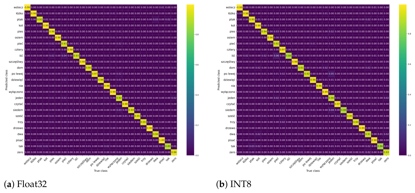
). As discussed in Section 5, parameter count alone is not predictive of accuracy in this regime: the largest model (CNN) is in fact the least accurate, indicating that the inductive bias of each architecture family, rather than raw capacity, is the dominant factor.

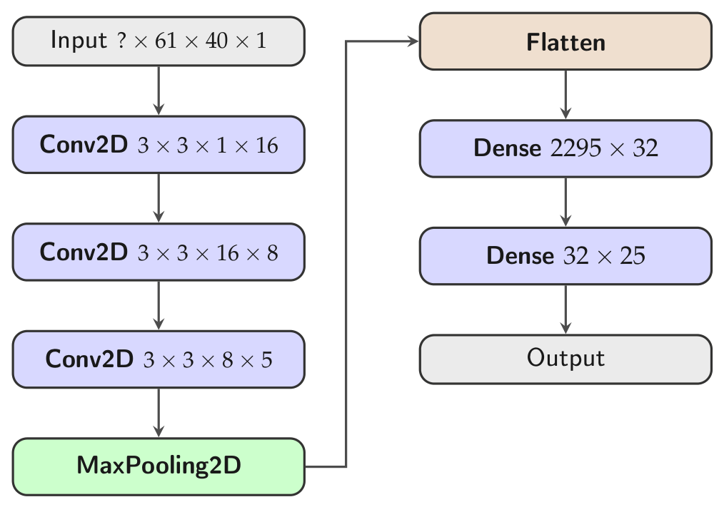
The CNN model is designed to function as an acoustic feature extractor. The model architecture is shown in Figure 3. The architecture utilizes standard two-dimensional convolutional layers to capture local time–frequency correlations, such as formants and pitch shifts. The multidimensional output is subsequently flattened and processed through fully connected dense layers, culminating in a softmax classifier that outputs the target vocabulary probabilities.

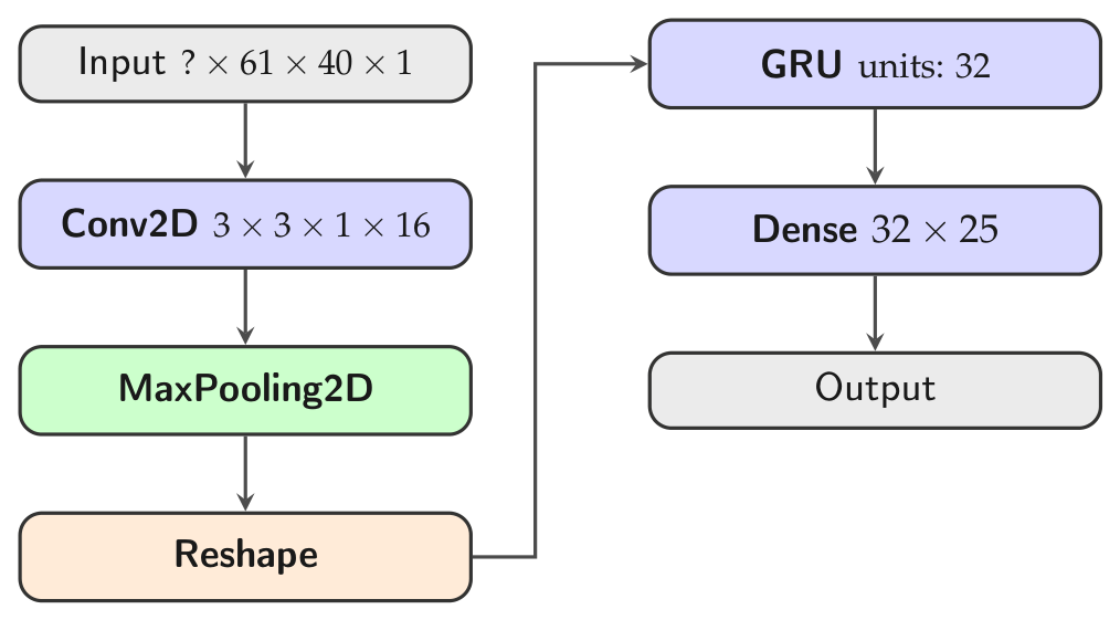
To better capture the sequential nature of speech, a hybrid CRNN architecture was implemented (Figure 4). The initial convolutional layer forms a spatial front end that reduces the input dimensionality. Next, the spatial dimensions are flattened while the temporal axis is preserved, forming a time-series representation. This is fed into a single GRU layer with 32 units (see Figure 4), which allows the model to capture long-term phonetic dependencies. The final layer is a dense classification layer with a softmax activation function.

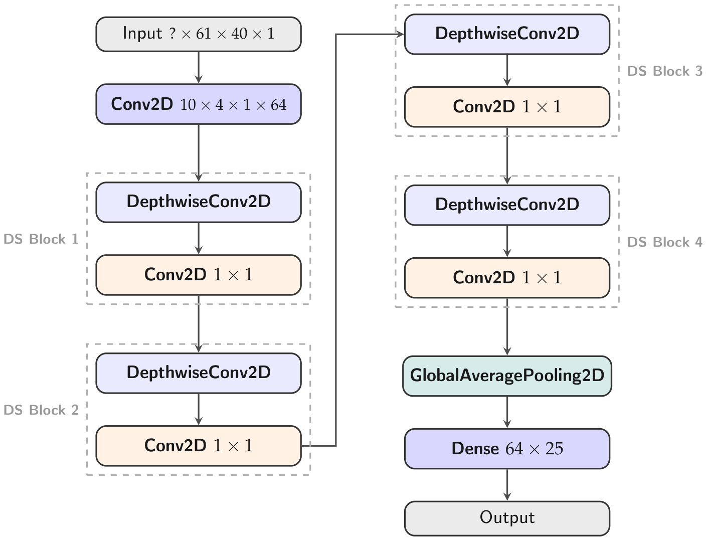
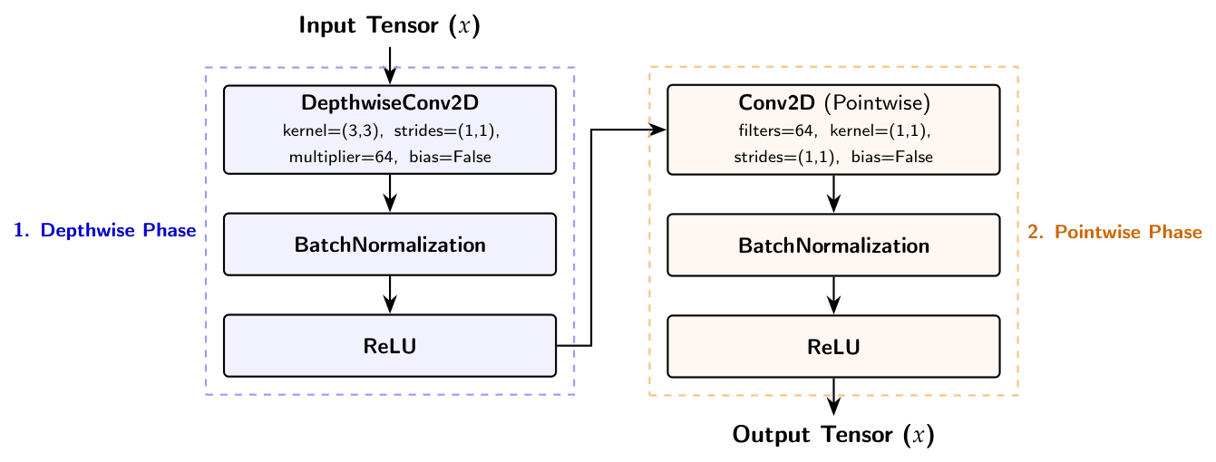
The DS-CNN architecture design is based on [3]. Model structure is shown in Figure 5. The model contains 4 DS blocks (Figure 6). Each block consists of a depthwise phase and a pointwise phase. In the depthwise part, a spatial filtering step applies a $3\times 3$ kernel independently to each input channel. It is followed by batch normalization for training stabilization and a ReLU activation function. In the pointwise part, a $1\times 1$ convolution is used to linearly combine the feature maps generated by the depthwise phase into output channels. As in the first phase, it is followed by batch normalization and a ReLU activation function. Formally, a depthwise separable convolution factorizes a standard convolution into a depthwise and a pointwise step. For an input with $C_{\mathrm{in}}$ channels, $C_{\mathrm{out}}$ output channels, and a $D_k\times D_k$ kernel applied to feature maps of spatial size $D_f\times D_f$, a standard convolution costs $D_k^2{C}_{\mathrm{in}}{C}_{\mathrm{out}}{D}_f^2$ multiply–accumulate operations, whereas the depthwise separable form costs $D_k^2{C}_{\mathrm{in}}{D}_f^2+C_{\mathrm{in}}{C}_{\mathrm{out}}{D}_f^2$. The resulting reduction factor is

$${\displaystyle \frac{D_k^2{C}_{\mathrm{in}}{D}_f^2+C_{\mathrm{in}}{C}_{\mathrm{out}}{D}_f^2}{D_k^2{C}_{\mathrm{in}}{C}_{\mathrm{out}}{D}_f^2}}={\displaystyle \frac{1}{C_{\mathrm{out}}}}+{\displaystyle \frac{1}{D_k^2}},$$

(4)

which, for the $3\times 3$ kernels used here, gives close to a ninefold reduction in cost and motivates the use of the DS-CNN for microcontroller deployment.

For completeness, we give the forward-propagation equations of the three proposed models, using the notation of Section 3 (input $X\in {\mathbb{R}}^{T\times K}$, logits $\mathbf{z}$, and posteriors $\mathbf{p}=\mathrm{softmax}\left(\mathbf{z}\right)$ from Equation (1)).

CNN. With $A^{\left(0\right)}=X$, each convolutional layer $l=1,2,3$ computes

$$A^{\left(l\right)}=\mathrm{ReLU}\left(W^{\left(l\right)}\ast A^{(l-1)}+{\mathbf{b}}^{\left(l\right)}\right),$$

(5)

where ∗ denotes two-dimensional convolution. Max pooling and flattening yield $\mathbf{v}=\mathrm{flatten}\left(\mathrm{MaxPool}\left(A^{\left(3\right)}\right)\right)$, which two fully connected layers map to the logits,

$$\mathbf{h}=\mathrm{ReLU}(W_1\mathbf{v}+{\mathbf{b}}_1),\mathbf{z}=W_2\mathbf{h}+{\mathbf{b}}_2.$$

(6)

CRNN. A single convolution and pooling stage produces a feature map that is reshaped along the time axis into a sequence $({\mathbf{x}}_1,\dots ,{\mathbf{x}}_T)$ with ${\mathbf{x}}_t\in {\mathbb{R}}^d$. For $t=1,\dots ,T$, the 32-unit GRU with hidden state ${\mathbf{h}}_t$ updates

$$\begin{array}{cc}\hfill {\mathbf{r}}_t& =\sigma (W_r{\mathbf{x}}_t+U_r{\mathbf{h}}_{t-1}+{\mathbf{b}}_r),\hfill \end{array}$$

(7)

$$\begin{array}{cc}\hfill {\mathbf{u}}_t& =\sigma (W_u{\mathbf{x}}_t+U_u{\mathbf{h}}_{t-1}+{\mathbf{b}}_u),\hfill \end{array}$$

(8)

$$\begin{array}{cc}\hfill {\tilde{\mathbf{h}}}_t& =\tanh \left(W_h{\mathbf{x}}_t+U_h({\mathbf{r}}_t\odot {\mathbf{h}}_{t-1})+{\mathbf{b}}_h\right),\hfill \end{array}$$

(9)

$$\begin{array}{cc}\hfill {\mathbf{h}}_t& =(1-{\mathbf{u}}_t)\odot {\tilde{\mathbf{h}}}_t+{\mathbf{u}}_t\odot {\mathbf{h}}_{t-1},\hfill \end{array}$$

(10)

where $\sigma$ is the logistic sigmoid and ⊙ the Hadamard product. The final hidden state gives the logits $\mathbf{z}=W_o{\mathbf{h}}_T+{\mathbf{b}}_o$.

DS-CNN. An initial standard convolution produces ${\mathbf{A}}^{\left(0\right)}$. Each DS block $b=1,\dots ,4$ applies a depthwise ($\mathrm{DW}$) and then a pointwise ($\mathrm{PW}$) convolution, each followed by batch normalization ($\mathrm{BN}$) and a ReLU activation,

$$\begin{array}{cc}\hfill U^{\left(b\right)}& =\mathrm{ReLU}\left(\mathrm{BN}\left(\mathrm{DW}\left(A^{(b-1)}\right)\right)\right),\hfill \end{array}$$

(11)

$$\begin{array}{cc}\hfill A^{\left(b\right)}& =\mathrm{ReLU}\left(\mathrm{BN}\left(\mathrm{PW}\left(U^{\left(b\right)}\right)\right)\right).\hfill \end{array}$$

(12)

Global average pooling over the spatial dimensions $H\times W$ yields $\mathbf{g}={\displaystyle \frac{1}{HW}}{\sum }_{i,j}{A}_{i,j,:}^{\left(4\right)}$, which a dense layer maps to the logits $\mathbf{z}=W_o\mathbf{g}+{\mathbf{b}}_o$.

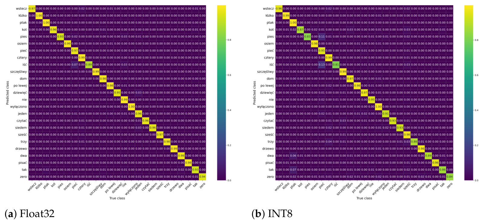
While each architecture follows an established family, the specific instantiations reported here constitute our design contribution. For the CNN, we adopt a three-layer convolutional stack with decreasing channel widths (16, 8, 5) followed by a two-layer classifier, trading depth for a small parameter count. For the CRNN, we reduce the convolutional front end to a single convolution–pooling stage feeding a single 32-unit GRU, which we found sufficient to model the temporal context of one-second commands at minimal cost. For the DS-CNN, we fix four depthwise-separable blocks with a channel multiplier of 64 and no inter-block spatial downsampling, prioritizing accuracy retention under quantization. All three architectures were tuned to a comparable budget on the order of ${10}^4$ parameters, such that the cross-architecture comparison in Section 5 reflects inductive bias rather than raw capacity. The exact per-layer configurations, which are the design variables we set, are given in Figure 3, Figure 4 and Figure 5, and the resulting parameter counts in Table 1.

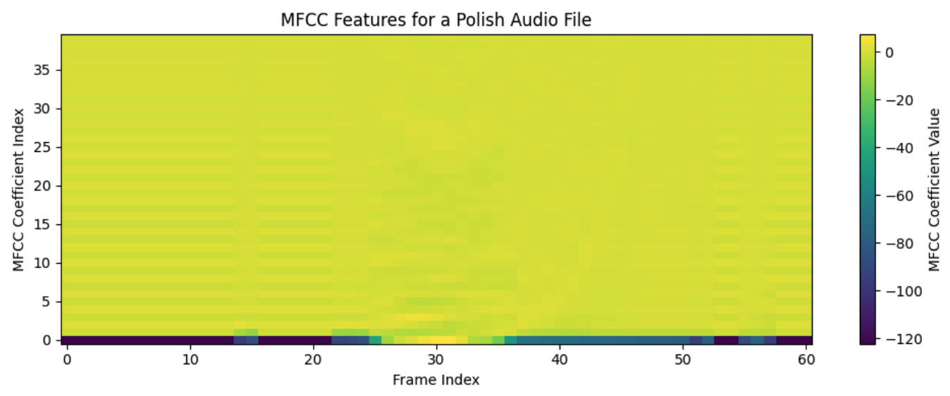
The feature-extraction and input hyperparameters were chosen to match the dataset and the microcontroller budget rather than tuned to the target language. Each one-second clip is represented by a $61\times 40$ MFCC matrix (61 time frames of 40 coefficients). The MFCC front end uses 40 Mel filter banks spanning 64–8000 Hz, a 512-point FFT at a 16 kHz sampling rate, and 50% frame overlap; the 512-point window corresponds to a frame length of 32 ms, and the 50% overlap gives a frame shift of 16 ms, which yields $\lfloor (1000\mathrm{ms}-32\mathrm{ms})/16\mathrm{ms}\rfloor +1=61$ frames per one-second clip. A single static feature stream, without delta or delta-delta coefficients, was retained to limit the input size and the resulting model and tensor-arena memory on the RP2350. We did not tune the number of Mel filters, the number of coefficients, or the frame length and shift to the Polish phoneme inventory, nor did we evaluate dynamic (delta) features. Because Polish phoneme confusability is concentrated in fine spectral detail (owing to its rich fricative and sibilant inventory), a targeted study of these feature choices, including a higher Mel resolution and the addition of delta coefficients, is a promising route to better discrimination of pairs such as “ptak”/“tak” and is left for future work. Similarly, the 32-unit GRU of the CRNN was sized to meet the shared parameter budget rather than selected by an exhaustive search; we did not systematically explore whether a larger recurrent state would improve accuracy at the cost of latency or whether performance is already saturated on this 25-word vocabulary.

The complete on-device inference pipeline is summarized in Algorithm 1; the Float32 and INT8 variants differ only in the input-quantization step.

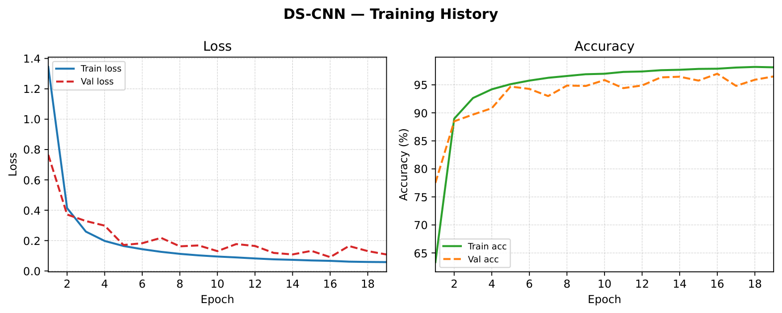
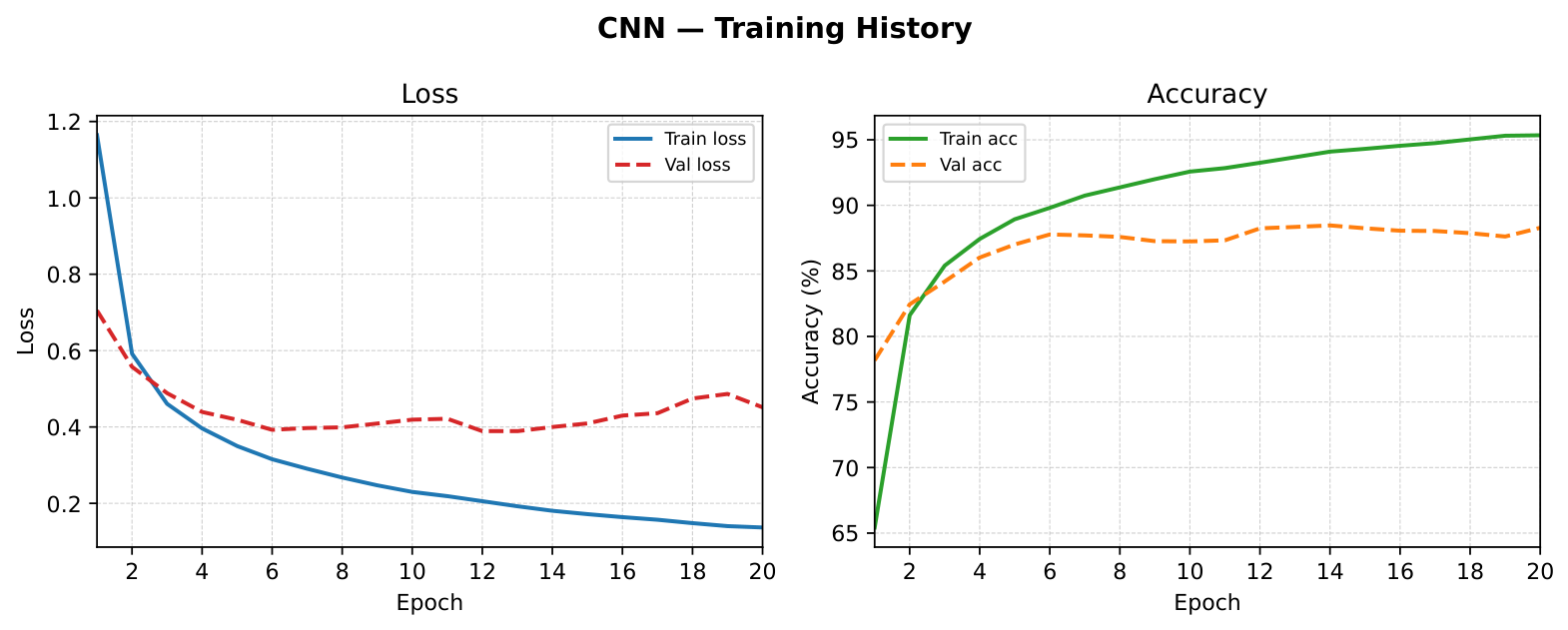
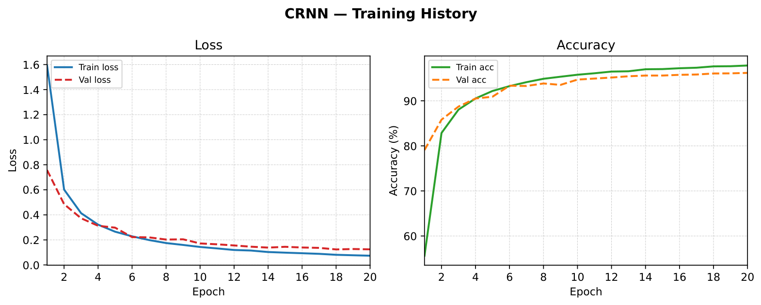
The CNN, CRNN, and DS-CNN models were trained using the Adam optimizer with sparse categorical cross-entropy loss over a maximum of 20 epochs, with a batch size of 64 or 128 (model-dependent) and early stopping (patience = 3, restoring best weights). Because early stopping restored the weights from the epoch of lowest validation loss, the 20-epoch cap acts only as an upper bound: the reported accuracies correspond to the best-validation (converged) checkpoint rather than to premature stopping. 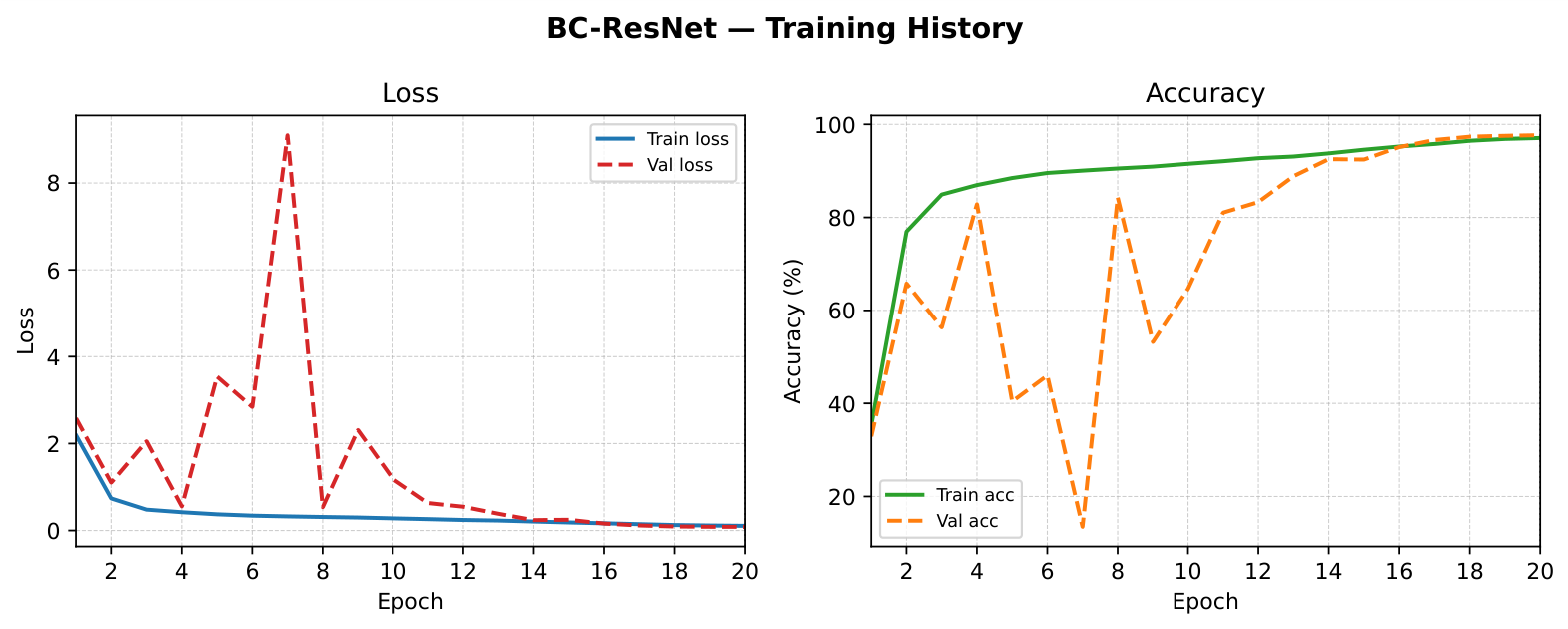The learning curves are available in Appendix B.

Algorithm 1 On-device keyword-spotting inference on the RP2350.

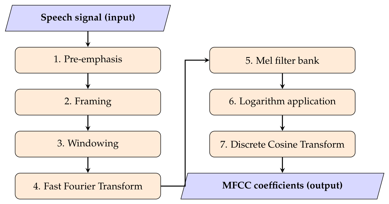
Require: raw audio frame s (1 s, 16 kHz); trained model $f_{\theta }$ (Float32 or INT8); threshold $\tau$; for the INT8 model, input scale S and zero point Z Ensure: recognized keyword or reject   1: $\mathbf{X}\leftarrow ExtractMFCC\left(s\right)$▹ pre-emphasis, framing, windowing, FFT, Mel filter bank, log, DCT (CMSIS-DSP)   2: if $f_{\theta }$ is INT8 then   3:     $\mathbf{X}\leftarrow \mathrm{round}(\mathbf{X}/S)+Z$     ▹ quantize MFCC input to 8-bit   4:     $\mathbf{z}\leftarrow f_{\theta }\left(\mathbf{X}\right)$▹ integer forward pass (TFLite Micro/CMSIS-NN); logits dequantized to ${\mathbb{R}}^N$   5: else   6:     $\mathbf{z}\leftarrow f_{\theta }\left(\mathbf{X}\right)$          ▹ floating-point forward pass   7: end if   8: p ← softmax$\left(\mathbf{z}\right)$               ▹ Equation (1)   9: $\widehat{y}\leftarrow \arg {\max }_i{p}_i$ 10: if $p_{\widehat{y}}\ge \tau$ then 11:     return keyword $\widehat{y}$ 12: else 13:     return reject       ▹ background noise or unknown word 14: end if

The BC-ResNet model followed the training procedure from the original paper [8]: an SGD optimizer with momentum 0.9, L2 weight decay 0.001, an initial learning rate of 0.1 with a 2-epoch warmup and cosine/stepwise decay, over 20 epochs with a batch size of 128. The three proposed models were thus trained under identical conditions so that comparisons among them (the primary object of this study) are controlled. The BC-ResNet reference was instead trained according to its authors’ procedure to reproduce its reported state-of-the-art behavior faithfully; imposing our generic training setup on it could have handicapped the reference and caused its performance to be underestimated. We note that this difference in training protocol is a confounding factor for the BC-ResNet comparison specifically, which we discuss further in the limitations (Section 6).

The dataset was partitioned into a training subset (80%, 112,677 samples) and a test subset (20%, 28,169 samples) using a fixed random seed. The split was not explicitly speaker-independent. Fivefold cross-validation was applied on the training subset for model selection; final accuracy was evaluated on the shared test set.

Regularization was applied in the form of early stopping on validation loss (CNN, CRNN, DS-CNN) and L2 weight decay (BC-ResNet). Data augmentation in the form of white noise injection was applied to the training set only; additional augmentations (pitch shifting, time stretching, and noise) were provided by the dataset authors. All training was performed in TensorFlow 2.10.1/Keras 2.10.0 (CNN, CRNN, DS-CNN) and PyTorch 2.5.1 (BC-ResNet) on a single NVIDIA GeForce GTX 1050 Ti GPU. The BC-ResNet model was subsequently exported to TensorFlow, such that all four models share an identical conversion, INT8 quantization, and on-device inference path; the only difference for BC-ResNet is thus on the training side (framework and procedure), not in the quantization or inference pipeline.

The total number of parameters for each architecture is summarized in Table 1.

4.2. Use of Generative AI Tools

A generative AI–based assistant (Claude 4.8; product details are given in the Acknowledgments) was used to support several parts of this work. In the software development, it assisted with debugging, with drafting helper functions and scripts, and with code validation; all AI-generated code was carefully reviewed and tested by the authors before use. In the preparation of the manuscript, it was used to improve the language of the text (grammar, vocabulary, and overall readability); to assist with the layout and style of the document; to help validate the mathematical formulas, and to perform final consistency checks across the text, figures, and tables. All AI-assisted code, text, and derivations were reviewed and verified by the authors, who take full responsibility for the content, the methods, and the results reported in this paper. The product details of the tools used are given in the Acknowledgments.

5. Results

5.1. Hardware Architecture

In order to investigate the performance of the proposed neural networks in a real-world scenario, a dedicated hardware platform was developed. The system architecture revolves around the Raspberry Pi Pico 2 development board, which features the RP2350 microcontroller (Figure 7). The RP2350 is a high-performance system on a chip (SoC) that employs a unique dual-core, dual-architecture design, providing two Arm Cortex-M33 cores and two RISC-V Hazard3 cores, both operating at a nominal frequency of 150 MHz [21].

In this research, the Arm Cortex-M33 cores were selected due to support for TinyML workloads, such as CMSIS-DSP [22] and Tensorflow Lite for Microcontrollers [18]. The Cortex-M33 implements the Armv8-M architecture, which includes Digital Signal Processing (DSP) instructions and a Single-Precision Floating-Point Unit (FPU). These hardware features are critical for efficient keyword spotting (KWS), as they allow the accelerated computation of Mel-frequency cepstral coefficients (MFCCs) and optimize the execution of quantized neural network kernels. The microcontroller is equipped with 520 KB of on-chip SRAM. The Pico 2 board also provides 4 MB of external QSPI Flash memory [21].

The hardware implementation includes a custom dual-layer printed circuit board (PCB) designed and fabricated to interface the Raspberry Pi Pico 2 with an analog audio front end. This front end utilizes an electret microphone coupled with a low-noise pre-amplifier stage [23] to capture voice commands.

5.2. Testing on the Database

For testing the models, the dataset described in [9] was used. The database contains 1 s voice recordings of single words in 15 languages. All records have been augmented using time shifting, noise injection, pitch variation, etc. [9]. For testing, only Polish words were selected. The models were trained to recognize 25 classes, which are shown in

Table 2. List of Polish words used in experiments.

Word (in English)	Word (in Polish)	Count
backward	wstecz	918
bed	łóżko	4908
bird	ptak	1224
cat	kot	4362
dog	pies	5152
eight	osiem	4884
five	pięć	5164
four	cztery	5086
go	iść	5130
happy	szczęśliwy	4902
house	dom	5004
left	po lewej	1020
nine	dziewięć	4896
no	nie	31,086
off	wyłączono	3236
one	jeden	5612
read	czytać	4882
seven	siedem	4986
six	sześć	5008
three	trzy	5266
tree	drzewo	4380
two	dwa	5320
write	pisać	4816
yes	tak	8480
zero	zero	5124

.

The overall performance and memory requirements of the evaluated neural network architectures were measured in their Float32 format and after integer quantization (INT8).

Table 3. Performance of the evaluated models in Float32 (full-precision) format: classification accuracy, F1-score, model size, and mean on-device inference time on the Raspberry Pi Pico 2 (mean of 100 trials per model). The best value in each column is shown in bold.

Model	Accuracy (%)	F1-Score	Size (KB)	Inference Time (ms)
BC-ResNet	97.81	0.9780	104.98	579.1
DS-CNN	97.06	0.9707	98.85	1693.7
CRNN	96.19	0.9620	218.79	347.9
CNN	88.68	0.8869	300.64	357.7

and

Table 4. Performance of the evaluated models after INT8 quantization: classification accuracy, F1-score, model size, and mean on-device inference time on the Raspberry Pi Pico 2 (mean of 100 trials per model). The best value in each column is shown in bold.

Model	Accuracy (%)	F1-Score	Size (KB)	Inference Time (ms)
BC-ResNet	92.73	0.9258	101.97	501.9
DS-CNN	93.13	0.9331	46.15	311.3
CRNN	94.28	0.9431	182.62	150.3
CNN	85.32	0.8542	79.44	107.5

summarize the accuracy, F1-score, model size, and on-device inference time for the Float32 and INT8 variants, respectively. For all reported F1-scores, the weighted-averaged was computed across classes (each class’s F1 weighted by its number of samples), and no class weighting or oversampling was applied during training. Because the dataset is markedly imbalanced (e.g., “no”(“nie”) with 31,086 samples versus “backward” (“wstecz”) with 918), both the overall accuracy and the weighted F1-score are dominated by the most frequent classes and can mask poor performance on rare keywords; the per-class analysis of Figure 8 is therefore reported to give a more balanced view of per-keyword performance. As point estimates on a test set of roughly $28,000$ samples, the reported accuracies are statistically stable: the half-width of the $95\%$ Wald confidence interval does not exceed $\pm 0.4$ percentage points (for example, $\pm 0.27$ pp at $94\%$ accuracy), and so overlapping intervals do not affect the reported rankings.

The highest accuracy in Float32 format was achieved by the BC-ResNet model (97.81%), followed closely by DS-CNN (97.06%) and CRNN (96.19%). The CNN architecture exhibited the lowest Float32 accuracy at 88.68%. After INT8 quantization, the CRNN model retained the highest accuracy (94.28%), while BC-ResNet experienced the largest absolute accuracy drop (5.08 percentage points). Quantization significantly reduced the model size for the CNN (from 300.64 KB to 79.44 KB) and DS-CNN (from 98.85 KB to 46.15 KB). The file sizes of the CRNN and BC-ResNet architectures remained largely unaffected by the quantization process. Inference time was measured directly on the target hardware platform, the Raspberry Pi Pico 2 microcontroller, as the mean over 100 consecutive inferences per model; all programs were compiled with Releaseoptimization settings. The reported times measure the neural-network forward pass only and exclude MFCC feature extraction, which is a fixed additive cost common to all models; a full end-to-end budget would add this constant term to every entry. The standard deviation did not exceed $0.5$ $\mathrm{m}$$\mathrm{s}$ for any configuration and is therefore omitted. The resulting on-device latencies are reported alongside the accuracy and memory metrics in Table 3 and Table 4.

The shortest mean inference time was recorded for the CNN model in INT8 format ($107.5$ $\mathrm{m}$$\mathrm{s}$). The DS-CNN architecture exhibited the greatest relative speedup following INT8 quantization, with the mean inference time reduced from $1693.7$ $\mathrm{m}$$\mathrm{s}$ to $311.3$ $\mathrm{m}$$\mathrm{s}$ (approximately 5.4-fold). In contrast, the BC-ResNet architecture showed the smallest relative improvement after quantization, with execution time decreasing from $579.1$ $\mathrm{m}$$\mathrm{s}$ to $501.9$ $\mathrm{m}$$\mathrm{s}$. Relative to the one-second analysis window of the input frame, all INT8 models meet the real-time constraint, with inference well below 1 $\mathrm{s}$. In Float32, only the CNN and CRNN remain within this budget, whereas the DS-CNN ($1693.7$ $\mathrm{m}$$\mathrm{s}$) exceeds it and is therefore unsuitable for continuous, always-on operation unless quantized.

5.3. Comparison with Prior Work

To the best of our knowledge, no prior small-footprint KWS results exist for Polish, and so a direct, controlled comparison is not possible.

Table 5. Contextual comparison with representative small-footprint KWS studies. Prior results are on the English Google Speech Commands (GSC) dataset; the present work targets a 25-class Polish vocabulary. Accuracies refer to full-precision (Float32) models and are not directly comparable across datasets and languages.

Study	Architecture	Dataset (Language, Classes)	Accuracy (%)
Zhang et al. [3]	DS-CNN	GSC (English, 12)	95.4
Kim et al. [8]	BC-ResNet-1	GSC (English, 12)	96.6
This work	BC-ResNet (reference)	Polish, 25	97.81
This work	DS-CNN (proposed)	Polish, 25	97.06
This work	CRNN (proposed)	Polish, 25	96.19
This work	CNN (proposed)	Polish, 25	88.68

instead places our full-precision results in the context of representative English-language small-footprint KWS studies evaluated on the Google Speech Commands benchmark. Two observations follow. First, our reimplementation of BC-ResNet reaches 97.81% on the 25-class Polish task, in the same range as the 96.6% reported by its authors on the 12-class English benchmark [8], which supports the validity of our training and evaluation setup. Second, the proposed CRNN and DS-CNN attain accuracies comparable to these state-of-the-art English models while operating on a larger (25-class) and phonetically harder vocabulary. We stress that these numbers are not directly comparable, as the language, vocabulary size, and recording conditions differ; the table is intended for context rather than as a head-to-head benchmark.

5.4. Confusion Matrix

Confusion matrices were generated for all evaluated models to assess prediction stability across individual voice commands. In every matrix, rows correspond to the true class and columns to the predicted class, and so a strong diagonal indicates correct predictions. For readability, the main text summarizes per-class behavior through the accuracy view of Figure 8, while the full per-model confusion matrices, for all four models in both Float32 and INT8 formats, are collected in Appendix A.

To compare per-class behavior across all models and formats at a glance, Figure 8 reports the per-class accuracy, that is, the diagonal of each confusion matrix, with keywords ordered from hardest to easiest. It shows that a small set of phonetically confusable keywords, led by “ptak” (“bird”), concentrates the errors, and that INT8 quantization amplifies these weaknesses most severely for BC-ResNet (whose accuracy on “ptak” falls to 40%) and for the CNN, whereas the CRNN and DS-CNN degrade more gracefully. This view also highlights that the unweighted (macro) per-class accuracy is lower than the sample-weighted accuracy of Table 4 for the fragile models, confirming that their degradation is concentrated in the rarer, phonetically hard classes.

The BC-ResNet model demonstrated robust word recognition performance across the majority of classes in Float32 format. A notable exception was the keyword “bird” (“ptak”), which achieved 83.5% per-class accuracy and was most frequently misclassified as “yes” (tak) in 7.4% of cases and as “two” (“dwa”) in 4.9% of cases.

In the Float32 CNN model, the lowest classification accuracy was recorded for the command “bird” (“ptak”) at 70.8%, which was misclassified as yes (tak) in 16.9% of instances. A further notable error involved the keyword “seven” (“siedem”), which achieved only 72.7% accuracy and was most frequently confused with “four” (“cztery”) in 13.3% of cases.

The Float32 CRNN model exhibited generally strong per-class performance. The weakest classes were “yes” (“tak”) at 89.1%, “one” (“jeden”) at 91.7%, and “go” (“iść”) at 92.6%; the latter was occasionally misclassified as “five” (“pięć”) in 3.6% of cases.

In the Float32 DS-CNN model, the weakest class was “go” (“iść”) at 88.8%, which was most frequently misclassified as five (pięć) in 6.7% of instances. The remaining classes maintained uniformly high per-class accuracy.

Following INT8 quantization, the BC-ResNet model exhibited a substantial accuracy degradation for the keyword “bird” (“ptak”), which fell to 39.9%. This word was most frequently recognized as “yes” (“tak”) (24.3%), “two” (“dwa”) (16.9%), and “four” (“cztery”) (7.4%), representing the most pronounced per-class degradation observed across all quantized models.

In the quantized CNN model, the keyword “bird” (“ptak”) dropped to 61.7%, with “yes” (“tak”) accounting for 21.0% of misclassifications. The class “seven” (“siedem”) also declined to 68.7% accuracy, primarily due to confusion with “four” (“cztery”) in 14.7% of cases.

For the quantized CRNN architecture, the majority of classes maintained satisfactory accuracy. The weakest classes were “yes” (“tak”) at 85.9%, “seven” (“siedem”) at 87.7% (confused with “one” (“jeden”) in 4.1% of cases), and “go” (“iść”) at 87.8% (confused with “five” (“pięć”) in 5.9% of cases).

In the quantized DS-CNN model, the weakest class was “go” (“iść”) at 80.9%, most frequently misclassified as “five” (“pięć”) in 13.4% of instances. The class “dog” (“pies”) also declined to 82.6% accuracy, with the primary source of confusion being “five” (“pięć”) in 10.6% of cases.

6. Discussion

Experimental results demonstrate that deploying high-accuracy keyword spotting (KWS) on a resource-constrained microcontroller like the RP2350 requires navigating various trade-offs. No single model excelled across all metrics, which included full-precision accuracy, robustness to INT8 quantization, memory footprint, and inference speed. Instead, each architecture offers distinct advantages, meaning the best choice depends heavily on the specific constraints of the target application.

In the full-precision (Float32) tests, the BC-ResNet model achieved the highest accuracy at 97.81% while remaining highly parameter-efficient, utilizing only 13,450 parameters. The DS-CNN and CRNN followed closely with scores of 97.06% and 96.19%, respectively. Conversely, the standard CNN lagged significantly at 88.68%, despite containing a massive 75,982 parameters. This confirms that architectures specifically designed for the time and frequency structures of speech, such as DS-CNN [3] and BC-ResNet [8], capture audio patterns far more effectively than generic convolutional layers.

When INT8 quantization was applied to compress the models, the robustness rankings inverted. The CRNN proved most resilient, losing only 1.91 percentage points (96.19% → 94.28%), making it the most accurate quantized model. The DS-CNN experienced a moderate drop (97.06% → 93.13%). The BC-ResNet, however, suffered the most significant decrease, losing 5.08 percentage points (97.81% → 92.73%). This fragility was particularly noticeable with phonetically similar keywords; for instance, the Polish command “ptak” (“bird”) dropped to a 39.9% accuracy rate, frequently being confused with “tak” (“yes”) and “dwa” (“two”) (see Figure A1b). All four models share the same inference and quantization pipeline: each was exported to TensorFlow, quantized to INT8 with the same post-training TensorFlow Lite converter and calibration procedure, and executed under the same TensorFlow Lite Micro runtime. Quantization tooling and inference-time numerical handling are therefore controlled across models, and the observed robustness differences are not attributable to different converters, calibration sets, or runtimes. The BC-ResNet reference does, however, differ on the training side, having been trained in PyTorch with its authors’ procedure rather than in TensorFlow/Keras; this may shape its learned weight and activation distributions and hence its quantization sensitivity, and we acknowledge it as a training-side confound, although it does not arise from the quantization pipeline itself. We further note that we did not isolate the individual contributions of layerwise quantization sensitivity or specific integer kernels. The architectural interpretation we offer is thus a plausible hypothesis rather than an established cause: BC-ResNet’s broadcasted residual operations rely on frequencywise spectral mappings whose reduced dynamic range under eight-bit arithmetic may erode fine spectral detail, whereas the CRNN’s reliance on temporal dynamics may be more tolerant of rounding. A controlled attribution, together with quantization-aware training and a layerwise sensitivity analysis, is left for future work.

The impact of quantization on memory footprint also varied by architecture. The CNN and DS-CNN compressed significantly, shrinking down to 79.44 KB and 46.15 KB, respectively, making the DS-CNN the smallest deployed model in the study. The CRNN compressed only modestly by 16.5% to 182.62 KB, remaining the largest quantized model, as a significant portion of its footprint is attributable to metadata and structural elements rather than core weights. Strikingly, the BC-ResNet barely compressed at all, merely changing from 104.98 KB to 101.97 KB. Because it already relies on very few parameters, its overall size is dominated by structural overhead rather than weight storage, meaning eight-bit weights offer almost no space savings. This demonstrates that quantization does not uniformly result in a fourfold size reduction; the actual savings depend heavily on the model’s architectural design.

Inference latency, measured directly on the RP2350 (Table 3 and Table 4), revealed further differences. The DS-CNN experienced the most significant speed improvement from quantization, dropping from $1693.7$ $\mathrm{m}$$\mathrm{s}$ to $311.3$ $\mathrm{m}$$\mathrm{s}$ (a 5.4× speedup). The standard CNN achieved the fastest quantized inference at $107.5$ $\mathrm{m}$$\mathrm{s}$; however, given its lower accuracy of 85.32%, it is better suited as a low-power trigger than as a primary recognizer. The CRNN provided a strong balance, combining the highest quantized accuracy with a competitive $150.3$ $\mathrm{m}$$\mathrm{s}$ latency. Conversely, the BC-ResNet gained minimal speed, shifting by a factor of only 1.15, from $579.1$ $\mathrm{m}$$\mathrm{s}$ to $501.9$ $\mathrm{m}$$\mathrm{s}$.

These differences are explained by the computational and memory profiles of the models, reported in

Table 6. Computational and memory characteristics of the evaluated TFLite models. “Operations” is the number of multiply–accumulate operations per inference, which is identical for the Float32 and INT8 variants of a model. “Intermediate buffers” is the total size of the intermediate tensors (a proxy for memory traffic), and “Peak buffer” is the largest single intermediate tensor (a proxy for the tensor-arena size). File sizes are reported in Table 3 and Table 4.

Model	Variant	Operations (M)	Intermediate Buffers (KiB)	Peak Buffer (KiB)
BC-ResNet	Float32	4.20	5797.7	95.3
	INT8		1474.4	29.8
DS-CNN	Float32	26.35	1561.5	155.0
	INT8		398.1	38.8
CRNN	Float32	2.52	492.8	140.1
	INT8		167.5	35.0
CNN	Float32	6.87	562.3	286.9
	INT8		579.0	288.6

: INT8 quantization mainly accelerates arithmetic, and so its benefit is largest for arithmetic-bound models and smallest for memory-bound ones. The DS-CNN performs by far the most arithmetic (26.35 M operations per inference), and so replacing floating-point with integer arithmetic yields a large gain, consistent with its 5.4-fold speed increase; its intermediate buffers also shrink substantially (from $1561.5$ KiB to $398.1$ KiB). In contrast, BC-ResNet performs comparatively few operations (4.20 M) yet allocates by far the largest intermediate buffers ($5797.7$ KiB in Float32), indicating that its runtime is dominated by memory movement rather than computation; quantization therefore yields only a modest 1.15-fold improvement despite its low parameter count. The CNN and CRNN lie between these extremes. This profile-based account replaces the earlier qualitative statement and directly attributes the differing latency reductions to the balance between arithmetic and memory operations in each architecture.

An analysis of classification errors across all architectures revealed a tendency to confuse words with similar phonetic structures. In the Polish dataset, “ptak” (“bird”) and “tak” (“yes”) share a near-identical vocalic nucleus and coda, while “iść” (“go”) was frequently confused with “pięć” (“five”). Such pairs become increasingly difficult to distinguish as the effective spectral resolution is lowered by quantization. This pattern suggests that while post-training quantization is sufficient for more robust architectures, quantization-aware training [10] would likely be necessary for sensitive models such as the BC-ResNet to preserve the subtle acoustic cues needed to separate these similar words.

Although this study targets Polish, the proposed pipeline is language-agnostic. The MFCC front end, the network architectures, and the quantization and deployment workflow do not depend on the target language; retargeting to another language requires only a labeled keyword corpus in that language and a change in the output vocabulary size N in Equation (1), with no change in the model structure. What varies across languages is the intrinsic difficulty of the vocabulary: as our error analysis shows, phonetically close keywords, which are especially abundant in consonant-rich Slavic languages such as Polish, are the main driver of errors and of quantization sensitivity. We therefore expect the architectural and quantization trends reported here to transfer to other languages, whereas the absolute accuracies will depend on the phonetic separability of the chosen keyword set.

The successful implementation on the custom PCB validated the RP2350 as a robust platform for TinyML. The ARM Cortex-M33 cores provided sufficient computational power, in particular by exploiting the DSP extension instructions of the Armv8-M architecture, which accelerate both the MFCC feature extraction (via the CMSIS-DSP library) and the quantized neural-network kernels (via the CMSIS-NN back end used by TensorFlow Lite for Microcontrollers). Future research could explore utilizing the dual-core capability of the RP2350 to pipeline the MFCC extraction and neural network inference stages, potentially decreasing latency further.

A key limitation of this study is that all reported metrics were obtained on the pre-recorded, augmented evaluation corpus rather than on live audio captured through the on-board acquisition chain. Consequently, the accuracy and F1-scores characterize the models together with the INT8 quantization and on-device latency behavior but not the complete microphone-to-decision pipeline. Preliminary tests using live input from the electret-microphone front end exhibited a marked degradation in recognition accuracy relative to the dataset evaluation. We attribute this gap primarily to a domain mismatch between the crowdsourced training corpus and the audio captured by the custom front end, rather than to the network architectures themselves, which performed consistently on in-domain data. Acoustic analysis of the raw recordings (

Table 7. Per-sample acoustic measurements obtained from the electret-microphone front-end recordings. SNR was estimated using the lowest-energy decile of $20\mathrm{ms}$ frames as a noise-floor proxy. Roll-off denotes the highest frequency bin within $20\mathrm{dB}$ of the spectral peak. No clipping was detected in any sample (<0.001%).

Sample (Polish)	Sample (English)	RMS (dBFS)	SNR (dB)	Roll-Off (Hz)
jeden	one	$-27.7$	$10.7$	1875
dwa	two	$-27.0$	$11.8$	1109
cztery	four	$-27.7$	$10.7$	1516
pięć	five	$-31.9$	$6.3$	1898
osiem	eight	$-29.4$	$8.7$	1586
dziewięć	nine	$-28.9$	$9.0$	1719
łóżko	bed	$-27.0$	$10.6$	742
Mean ± SD		$-28.6\pm 1.5$	$9.7\pm 1.7$	$1492\pm 393$

) is consistent with this attribution along two dimensions: the SNR, estimated from the lowest-energy decile of $20\mathrm{ms}$ frames (used as a noise-floor proxy in the absence of explicit silence segments), averaged $9.7\mathrm{dB}$ ($\sigma =1.7\mathrm{dB}$, range $6.3$–$11.8\mathrm{dB}$), well below the $20\mathrm{dB}$ threshold commonly required for reliable speech processing, and spectral analysis revealed a mean $-20\mathrm{dB}$ roll-off at $1.5\mathrm{kHz}$ ($\sigma =0.4\mathrm{kHz}$), far below the $4\mathrm{kHz}$ lower bound expected for narrowband-grade speech capture. Consistent RMS levels across recordings (range $4.9\mathrm{dB}$) and the absence of clipping make gain misconfiguration and front-end saturation unlikely as primary factors. We stress, however, that these measurements characterize the captured signal rather than isolate the individual contributions of the microphone, the analog front-end, the MFCC extraction, and ambient noise; we did not perform a controlled ablation that varies each factor independently, and so the attribution should be read as strongly supported by the signal statistics rather than as a fully isolated causal decomposition. Closing this gap will require a controlled front-end characterization that separates these factors, the collection of an in-domain dataset recorded directly through the target hardware, and the application of domain-adaptation techniques together with quantization-aware training; we regard this microphone-level validation as essential future work before the prototype can serve as a consumer-grade voice interface.

Beyond this microphone-level validation, several methodological factors bound the strength of our conclusions. First, the evaluation corpus is aggregated from crowdsourced recordings and does not expose speaker identifiers, and so a strictly speaker-disjoint training/test split was not possible; we therefore cannot fully exclude the possibility that some per-speaker characteristics are shared between the two partitions, which is known to inflate apparent accuracy in keyword spotting. The large and diverse pool of contributors and the heavy data augmentation mitigate but do not eliminate this risk, and a speaker-independent evaluation is an important direction for future work. Second, because all accuracies were obtained on this in-domain corpus, they should be interpreted as a controlled comparison of architectures and quantization schemes and as an upper bound on deployed performance, rather than as a prediction of live-microphone accuracy, which, as noted above, is currently degraded by the acquisition chain. Third, as discussed in Section 4, the BC-ResNet reference was trained with its authors’ procedure rather than our common protocol; this keeps the comparison fair to the reference but introduces a training-protocol confound, and so the relative findings among the three proposed models, which share an identical training setup, constitute the more controlled comparison. Fourth, we applied post-training quantization only, as the standard low-effort deployment path; quantization-aware training, which could recover much of the accuracy lost by sensitive models such as BC-ResNet, was outside the scope of this study and is a natural next step, ideally guided by a per-layer analysis of activation ranges and outlier weights to identify the most quantization-sensitive layers. Finally, we report inference latency but did not perform direct power profiling on the RP2350; for always-on operation, energy per inference (approximately the product of power and latency) is the ultimate metric, and a direct power characterization is an important complement to the latency measurements reported here.

7. Conclusions

This work presented a keyword-spotting pipeline for the Polish language, deployed and benchmarked on a severely resource-constrained microcontroller. Three compact architectures from the CNN, CRNN, and DS-CNN families were designed and benchmarked against the state-of-the-art BC-ResNet reference, both in full precision and after INT8 quantization, with latency measured directly on the Raspberry Pi Pico 2 (RP2350).

The results show that no single architecture is optimal across all deployment criteria. BC-ResNet achieved the highest full-precision accuracy (97.81%) but proved the most fragile under quantization, whereas the proposed CRNN was the most robust and the most accurate quantized model (94.28%), the DS-CNN yielded the smallest INT8 footprint (46.15 KB), and the CNN delivered the lowest latency ($107.5$ $\mathrm{m}$$\mathrm{s}$). Notably, the accuracy ranking inverted after quantization, the memory savings were highly non-uniform across architectures, and all quantized models met the one-second real-time budget on the target device. Error analysis further revealed that the dominant failure mode was the confusion of phonetically similar Polish words (e.g., “ptak”/“tak”, “iść”/“pięć”), which is exacerbated by the reduced numerical precision of INT8 arithmetic.

These findings provide practical guidance for selecting and quantizing small-footprint KWS models for Polish and other consonant-rich, morphologically rich languages. The principal open challenge is to bridge the gap between dataset-based evaluation and live microphone operation; addressing the acquisition-chain and domain-mismatch limitations discussed above, together with quantization-aware training, is the natural next step toward a deployable, always-on Polish voice interface.