A Comparative Study of VMD Methods Based on Different Optimization Algorithms in Non-Stationary Signal Decomposition of Bucket Runners

Abstract

Bucket runners are subjected to periodic discrete jet impacts during high-speed operation, yielding stress signals characterized by strong impact, wide bandwidth, and high non-stationarity, which demand high-frequency separation accuracy. Since VMD decomposition quality depends on the mode number K and the penalty factor α, empirical parameter selection for such non-stationary signals often leads to under-decomposition or modal aliasing. This study employs four metaheuristic algorithms—PSO, WOA, GWO, and SSA—to adaptively optimize VMD parameters. Eight evaluation metrics are established: the optimal mode number, optimized penalty factor, false mode number, over-decomposition score, under-decomposition score, under-decomposition proportion, residual energy proportion, and computation time. The experimental results demonstrate that SSA-VMD yields mode numbers consistent with true signal components and achieves a full over-decomposition score, a 33.33% under-decomposition ratio, and a 3.78% residual energy ratio, exhibiting the best comprehensive performance. In the stress signal decomposition of a hydropower station bucket runner, SSA-VMD extracts eight IMF components. After removing one false mode, the center frequencies of seven effective modes correspond to rotation frequency harmonics and structural natural frequencies, with a residual energy as low as 0.01%. These results verify the method’s effectiveness in non-stationary signal feature extraction.

1. Introduction

1.1. Research Background and Problem Statement

The bucket turbine has become the core equipment for the development of high-head hydraulic resources due to its high applicable head, wide range of high-efficiency operating conditions, and better operating stability under partial load than other models [1,2]. The runner is the core work component. When running at high speed, the runner is subjected to periodic impact of the discrete jet, which leads to a strong impact of the stress signal and a wide frequency band [3]. The runner stress signal contains a large amount of equipment state information. Accurately extracting fault features with a strong noise background is a core technical difficulty in condition monitoring and fault diagnosis of hydropower units [4,5].

Non-stationary stress signal analysis is a common means of mechanical fault diagnosis. The short-time Fourier transform is limited by the fixed window function, and it is difficult to balance the time-domain and frequency-domain resolution. Wavelet transform can do multi-scale analysis, which is more suitable for non-stationary signals than the Fourier transform. However, the selection of the wavelet basis lacks a unified standard, and the analysis results are easily affected by the basis function [6]. In 1998, Huang et al. [7] proposed empirical mode decomposition (EMD), which can adaptively decompose signals according to their own characteristics and provides a new idea for non-stationary signal processing. This method has been used to analyze the pressure fluctuation of pump turbines by the Hilbert–Huang transform [8]. Dai et al. [9] pointed out that adaptive signal decomposition technology is the key link of fault feature extraction. However, EMD has defects such as modal aliasing and endpoint effect, which limit the decomposition accuracy. Improved methods such as ensemble empirical mode decomposition (EEMD) alleviate modal aliasing to a certain extent and have been used in the field of turbocharger blade feature extraction [10]. Combined with EEMD and information entropy, Wang et al. [11] proposed a comprehensive evaluation method for pressure fluctuation in the draft tube of a Francis turbine. However, the EMD method still lacks a solid mathematical theory, and the recursive screening leads to the decomposition results not being unique, and the inherent defects have not been fundamentally solved.

Variational mode decomposition (VMD) is a non-recursive adaptive signal decomposition method proposed by Dragomiretskiy et al. in 2014. It decomposes signals by constructing and solving variational problems. Its frequency separation ability is better than that of EMD and the traditional wavelet transform [12]. VMD has been used in bearing fault diagnosis, vibration signal processing and pressure pulsation analysis of hydropower units [13,14,15]. The fault diagnosis method of VMD–Hilbert spectrum combined with deep learning also verifies the effectiveness of VMD in feature extraction [16]. However, the decomposition effect of VMD depends on the parameter settings, especially the mode number K and the penalty factor α. Too small a K will lead to under-decomposition, and different frequency components are mixed in the same intrinsic mode function. Too large a K will cause over-decomposition and produce false modal components. The penalty factor α determines the bandwidth of the modal components, which directly affects the decomposition accuracy [17]. The stress signal of bucket runners itself has a strong impact and a wide frequency band, which makes the selection of VMD parameters more sensitive. Parameter selection based on experience is prone to under-decomposition or modal aliasing. In the absence of prior knowledge, how to adaptively determine the optimal parameter combination has become a key issue that restricts the application of VMD engineering.

1.2. Research Progress and Existing Gaps

To solve this problem, a variety of swarm intelligence optimization algorithms are introduced into VMD parameter optimization. Particle swarm optimization (PSO) was proposed by Kennedy and Eberhart. As a classical swarm intelligence algorithm, PSO has a simple structure and fast convergence. It has been widely used in various fields [18]. Combining with other intelligent algorithms to optimize VMD parameters has also achieved a good noise reduction effect [19]. The whale optimization algorithm (WOA) was proposed by Mirjalili and Lewis. It simulates the predation behavior of humpback whales and has a good balance between global and local search [20]. It has achieved good results in combination with tabu search or applied to group decomposition parameter optimization [21,22]. The grey wolf optimization (GWO) algorithm was proposed by Mirjalili et al. It simulates the leadership level and hunting mechanism of grey wolves. It has fewer control parameters and is easy to implement [23]. It shows good optimization ability in VMD parameter optimization and has been applied to ultrasonic signal noise reduction, bearing fault diagnosis and other fields [24,25]. The sparrow search algorithm (SSA) was proposed by Xue and Shen to simulate the foraging and anti-predation behavior of sparrows. It has high computational efficiency and strong scalability. The related improved algorithms further improve its optimization performance [26,27,28]. In addition, new intelligent algorithms such as the seagull algorithm are also applied to VMD parameter optimization, which further enriches the selection of optimization methods [29]. In the field of hydropower units, VMD combined with the MOMEDA method has been used for bucket runner fault detection [30]. The influence of different optimization algorithms on the performance of the VMD-LSTM prediction model has also been compared [31]. The pressure pulsation prediction method based on VMD-LSTM further verifies the application value of optimization algorithms in hydraulic machinery signal processing [32]. However, the existing research mostly focuses on mixed-flow and axial-flow turbines or only verifies the combination effect of a single algorithm and VMD, and lacks horizontal comparison under a unified benchmark, which leads to the lack of a clear basis for the selection of intelligent algorithms in engineering applications. Especially for strong-impact non-stationary signals such as bucket runners, the optimization efficiency and decomposition accuracy of different algorithms are not clear, which directly affects the reliability of fault feature extraction.

1.3. Main Work and Contributions

Focusing on the demand for non-stationary signal decomposition of bucket runners, this paper selects four typical intelligent optimization algorithms, PSO, WOA, GWO and SSA, to construct VMD parameter adaptive optimization models. Then, through the decomposition experiment of the constructed signal and the measured non-stationary signal of bucket runners, the parameter optimization ability, convergence characteristics and decomposition accuracy of the four algorithms are compared under the unified experimental benchmark. The performance differences of the four optimization algorithms in the non-stationary signal decomposition of bucket runners are clarified, which provides a basis for the selection of adaptive optimization algorithms for VMD parameters of similar units.

2. Materials and Methods

All computations and simulations in this study were performed using GNU Octave (version 12.6.0, https://octave.org).

2.1. Outline

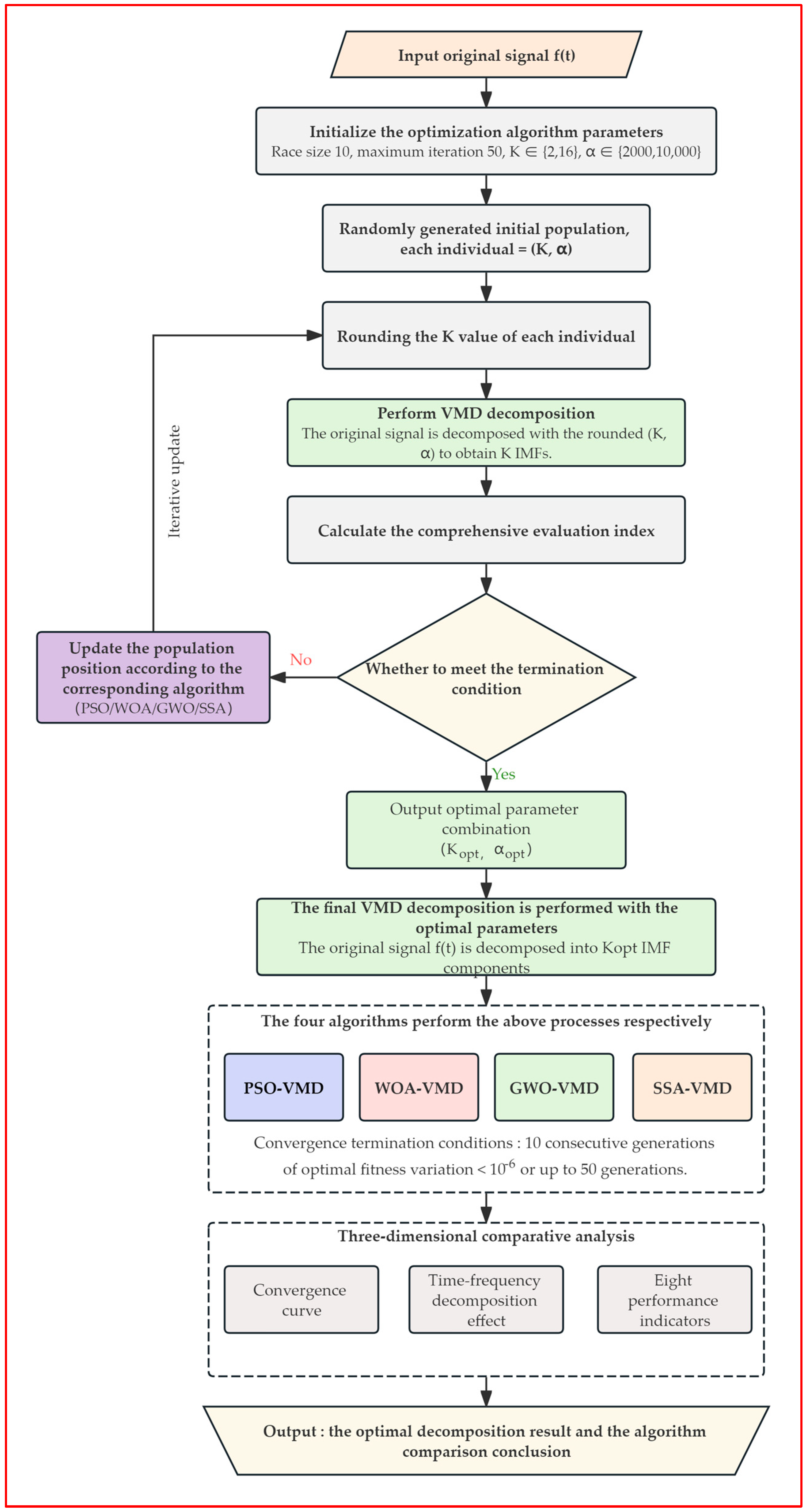
The core idea of this method is shown in Figure 1. The whole process is divided into three steps. Firstly, four swarm intelligence algorithms, PSO, WOA, GWO and SSA, are used to adaptively optimize the two key parameters of VMD, namely, the number of modes and the penalty factor. Then, the comprehensive evaluation index is minimized as the fitness function to drive the algorithm iteration. Finally, the optimal parameters obtained by optimization are used to perform VMD decomposition on the non-stationary signal of bucket runners, and the decomposition effects of the four algorithms are compared by multi-dimensional indicators.

2.2. Basic Principle of Variational Mode Decomposition

VMD transforms the signal decomposition problem into a constrained variational problem to solve and decomposes the original signal f(t) into K eigenmode functions u_k(t) with a finite bandwidth. Each mode is compactly distributed around its center frequency ω_k. The solution process of VMD includes two stages: variational problem construction and alternating direction multiplier method (ADMM) iterative solution.

2.2.1. The Construction of Variational Problems

The Hilbert transform is performed on each mode u_k(t) to obtain the analytical signal, and then the spectrum is moved to the baseband by the exponential term $e^{-j{\omega }_{k}t}$. The L2 norm of the demodulated signal gradient is used to measure the modal bandwidth, and the following constrained variational model is established:

$$\underset{\left\{u_k\right\},\left\{{\omega }_k\right\}}{\min }\left\{{\displaystyle \sum _{k=1}^K{‖{\partial }_t\left[\left(\delta \left(t\right)+\frac{j}{\pi t}\right)*u_k\left(t\right)\right]e^{-j{\omega }_{k}t}‖}_2^2}\right\}$$

(1)

$$s.t.{\displaystyle \sum _{k=1}^K{u}_k}\left(t\right)=f\left(t\right)$$

(2)

In the formula, {u_k} = {u₁, …, u_k} and {ω_k} = {ω₁, …, ω_k} represent the set of all modes and their center frequencies respectively; δ(t) is the Dirac function; j is the imaginary unit; ∂_t is the time derivative; and ${‖\cdot ‖}_2^2$ denotes the square of the L2 norm.

2.2.2. The Solution of Variational Problem

In order to solve the above constrained problem, the quadratic penalty term α and the Lagrangian multiplier λ(t) are introduced to form an unconstrained augmented Lagrangian function:

$$\begin{array}{l}L\left(\left\{u_k\right\},\left\{{\omega }_k\right\},\lambda \right)=\alpha {\displaystyle \sum _{k=1}^K{‖{\partial }_t\left[\left(\delta \left(t\right)+\frac{j}{\pi t}\right)*u_k\left(t\right)\right]e^{-j{\omega }_{k}t}‖}_2^2}\\ +{‖f\left(t\right)-{\displaystyle \sum _{k=1}^K{u}_k\left(t\right)}‖}_2^2+〈\lambda \left(t\right),f\left(t\right)-{\displaystyle \sum _{k=1}^K{u}_k\left(t\right)}〉\end{array}$$

(3)

where α controls the bandwidth constraint strength of each mode, λ(t) is used to strictly constrain the signal reconstruction accuracy, and $〈\cdot ,\cdot 〉$ represents the inner product.

The ADMM is used for iterative solution, and the modal component, center frequency and Lagrange multiplier are updated alternately in the frequency domain.

For the kth mode, its Fourier spectrum ${\widehat{u}}_k^{n+1}\left(\omega \right)$ is updated to

$${\widehat{u}}_k^{n+1}={\displaystyle \frac{\widehat{f}\left(\omega \right)-{\displaystyle {\sum }_{i\ne k}{\widehat{u}}_i\left(\omega \right)+\frac{\widehat{\lambda }\left(\omega \right)}{2}}}{1+2\alpha {\left(\omega -{\omega }_k^n\right)}^2}}$$

(4)

where $\widehat{f}\left(\omega \right)$, ${\widehat{u}}_i\left(\omega \right)$ and $\widehat{\lambda }\left(\omega \right)$ are the Fourier transform of the original signal, other modes and the Lagrange multiplier, respectively, and the superscript n is the number of iterations.

Formula (4) shows that the update of the mode is essentially Wiener filtering of the current residual signal, and the filtering characteristics are determined by α and ω_k.

The center frequency update formula is

$${\omega }_k^{n+1}={\displaystyle \frac{{\displaystyle {\int }_0^{\infty }\omega {\left|{\widehat{u}}_k^{n+1}\left(\omega \right)\right|}^{2}d\omega }}{{\displaystyle {\int }_0^{\infty }{\left|{\widehat{u}}_k^{n+1}\left(\omega \right)\right|}^{2}d\omega }}}$$

(5)

The decomposition quality of VMD is highly dependent on the values of K and α. If K is too small, it will lead to mode mixing, and if K is too large, it will produce false modes. If α is too large, it will be excessively smooth and lose details, and if α is too small, the noise suppression ability will be insufficient. The artificial experience trial-and-error method lacks adaptability, and it is difficult to ensure the stability of the decomposition effect under different signal conditions. This is the starting point for introducing intelligent optimization algorithms to automatically optimize parameters.

2.3. The Basic Principle of Optimization Algorithm

In this paper, four swarm intelligence optimization algorithms are selected as the tools for VMD parameter optimization. The core update mechanisms of each algorithm are given below.

2.3.1. Particle Swarm Optimization Algorithm

PSO simulates the foraging behavior of birds. Each particle i records its own historical optimal position p_i and the global optimal position g of the population, and updates the speed and position according to the following formula:

$$v_i\left(t+1\right)=\omega \cdot v_i\left(t\right)+c_1{r}_1\left[p_i\left(t\right)-x_i\left(t\right)\right]+c_2{r}_2\left[g\left(t\right)-x_i\left(t\right)\right]$$

(6)

$$x_i\left(t+1\right)=x_i\left(t\right)+v_i\left(t+1\right)$$

(7)

where ω is the inertia weight, c₁ and c₂ are learning factors, and r₁ and r₂ are random numbers in [0, 1].

PSO has a simple structure and few control parameters, but it is prone to premature convergence, and the optimization accuracy is limited in high-dimensional and multi-peak problems. In the VMD two-dimensional parameter (K, α) optimization scenario, the low-dimensional characteristics of PSO make its single-step iteration calculation small. However, because it only relies on two information sources of individual optimization and global optimization, it is easy to gather prematurely when there are multiple local minima, resulting in the search for the global optimal parameter combination.

2.3.2. Whale Optimization Algorithm

WOA simulates the bubble-net predation strategy of humpback whales, including three position update mechanisms.

Surrounding prey: With the current optimal individual as the prey, the search range is controlled by the attenuation parameter α:

$$D=\left|C\cdot X^{*}\left(t\right)-X\left(t\right)\right|,\hspace{1em}\hspace{1em}X\left(t+1\right)=X^{*}\left(t\right)-A\cdot D$$

(8)

where A = 2ɑ∙r-ɑ, C = 2r, r are random vectors in [0, 1], and ɑ decays linearly from 2 to 0.

Spiral update: Simulating whales approaching prey along a spiral path:

$$X\left(t+1\right)=D^{\prime }\cdot e^{bl}\cdot \cos \left(2\pi l\right)+X^{*}\left(t\right)$$

(9)

where D’ is the distance between the current individual and the optimal individual, b is the spiral shape constant, and l is the [−1, 1] random number.

Random search: When |A| ≥ 1, the individuals in the population are randomly selected as the reference update position to achieve global exploration.

In the iterative process, the surrounding or spiral mining is selected with a probability of 50%, and the parameter ɑ decays linearly from 2 to 0, achieving a smooth transition from global exploration to local mining. In the VMD parameter optimization, the spiral update mechanism makes WOA have strong local fine search ability on this continuous variable and can perform multi-directional exploration in the neighborhood of the optimal solution, which is conducive to jumping out of the local minimum point on the fitness surface.

2.3.3. Grey Wolf Optimization Algorithm

GWO divides the gray wolf population into four levels of α, β, δ and ω according to the fitness, and the first three jointly guide the search direction. The core update formula is

$$D_j=\left|C_j\cdot X_j\left(t\right)-X\left(t\right)\right|,\begin{array}{cc}& X_j\end{array}\left(t+1\right)=X_j\left(t\right)-A_j\cdot D_j,\hspace{1em}\hspace{1em}j\in \left\{\alpha ,\beta ,\delta \right\}$$

(10)

$$X\left(t+1\right)={\displaystyle \frac{X_{\alpha }+X_{\beta }+X_{\delta }}{3}}$$

(11)

where A = 2ɑ∙r₁ − ɑ, C = 2r₂, r₁, r₂ are random vectors in [0, 1], and ɑ decays linearly from 2 to 0. When |A| > 1, the population is dispersed for global exploration, and when |A| < 1, it gathers for local mining. In the VMD parameter optimization, the three-level leadership mechanism enables GWO to use the solutions of three different quality levels to guide the search direction at the same time, maintain good population diversity in the two-dimensional search space, and reduce the risk of falling into a local optimum due to the misleading of a single optimal solution.

2.3.4. Sparrow Search Algorithm

The SSA divides individuals into three types of roles: producer, follower and alerter.

Producer: The fitness is better, responsible for a wide-ranging search; the location is updated according to exponential decay; and the danger is quickly transferred to the safe area when it is found.

Followers: Individuals with poor fitness follow producers foraging; individuals in the latter part of the population flow to other areas for re-feeding due to insufficient energy.

Vigilance: An amount of 10%~20% of the population is responsible for the perception of danger. Individuals at the edge move closer to the safety center, and individuals in the center move randomly close to their peers.

The SSA realizes the dynamic switching between exploration and mining through multi-role division of labor. It has a fast convergence speed and high optimization accuracy and has excellent performance in benchmark tests and engineering optimization. In the VMD parameter optimization, the large-scale search of the producer is conducive to quickly locking the reasonable value range of K, and the fine tracking of the follower is conducive to fine-tuning α near the current optimal K, while the anti-predator mechanism of the alerter provides the ability to jump out of the local optimum. The characteristics of multi-role collaboration make it have a natural adaptation advantage for the mixed variable optimization of ‘discrete K + continuous α’.

2.4. An Adaptive VMD Parameter Selection Method Based on Optimization Algorithm

2.4.1. Optimize Variables and Range of Values

The number of modes K and the penalty factor α are selected as the variables to be optimized. K is an integer, with a value range of [2, 16]; α is a real number, with a value range of [2000, 10,000]. The lower limit of K is 2 to ensure that at least one modal component and residual can be separated. The upper limit is 16, taking into account the multi-component components that may exist in the stress signal of bucket runners and the calculation efficiency. The range of α is set according to the original VMD literature and the engineering experience of the turbine stress signal, covering the typical range from under-decomposition to over-decomposition, which meets the requirements of adaptive optimization search range.

PSO, WOA, GWO and SSA are continuous domain optimization algorithms, and K is a discrete integer variable. In this paper, the rounding and rounding discretization method is adopted: In each iteration, the algorithm updates the position according to the continuous variable. Before calculating the fitness, the K value is rounded and rounded and then substituted into the VMD decomposition to ensure that the number of modes used in each decomposition is a valid integer. This processing method is simple to implement and will not destroy the original continuous search mechanism of the algorithm.

In addition to K and α, VMD also contains other control parameters. In this paper, the original signal is first subjected to de-DC preprocessing, that is, the time-domain mean of the signal is subtracted to eliminate the interference of DC offset on the decomposition results. The remaining control parameters of VMD are set to fixed values: the Lagrange multiplier updates the step size τ = 0, the DC component is closed, the center frequency is initialized by a uniform distribution, and the convergence tolerance is set to 10⁻⁷. The above parameters remain fixed, and only K and α are used as optimization variables to ensure the uniqueness and reproducibility of the experimental variables.

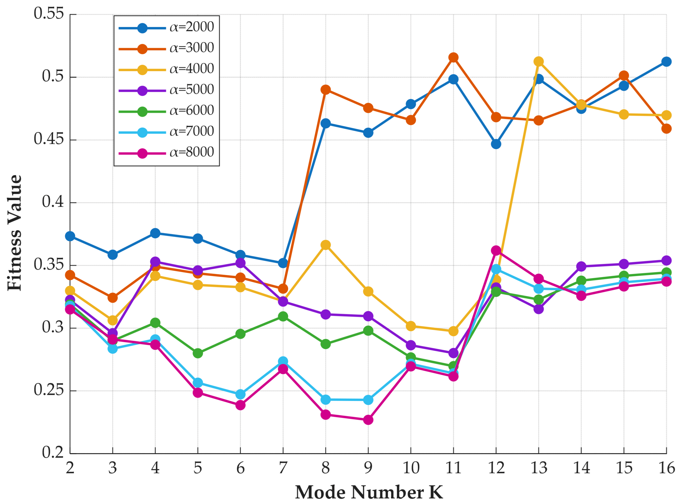
The impact of the rounding discretization was assessed through two analyses. First, the fitness landscape in the K dimension was examined by sweeping K from 2 to 16 at seven fixed α values (2000 to 8000). As shown in Figure 2, the fitness variation between adjacent integer K values is small (maximum absolute difference: 0.111), indicating a relatively smooth landscape rather than a harsh step function. Second, a direct comparison between continuous-domain optimization with rounding and pure integer-encoded optimization was performed over 30 independent runs. Both methods produce identical K_opt (8.0 ± 0.0), nearly identical α_opt (8598 ± 13 vs. 8600 ± 14; p = 0.519), and identical fitness values (0.2228). These results confirm that the rounding discretization does not impair the algorithms’ ability to locate the optimal parameters.

2.4.2. Fitness Function

In this paper, the comprehensive evaluation index is used as the fitness function, which is denoted as fitness1. For the K IMF components u_k(t)(k = 1, 2, …, K) obtained by VMD decomposition, the sample entropy of each component is first calculated. Sample entropy is a nonlinear dynamic index to measure the complexity and regularity of time series. The smaller the value is, the higher the self-similarity of the sequence is, the lower the noise content is, and the more regular the signal is. For the time series u_k(i)(i = 1, 2, …, N) with length N, the calculation steps of sample entropy are as follows:

Step 1: Construct a vector sequence with embedding dimension m:

$$U_k\left(i\right)=\left[u_k\left(i\right),u_k\left(i+1\right),\dots ,u_k\left(i+m-1\right)\right],\hspace{1em}\hspace{1em}i=1,2,\dots ,N-m+1$$

(12)

Step 2: Define the distance between vectors U_k(i) and U_k(j) as the maximum value of the difference between the corresponding elements:

$$d\left[U_k\left(i\right),U_k\left(j\right)\right]=\underset{r=0,1,\dots ,m-1}{\max }\left|u_k\left(i+r\right)-u_k\left(j+r\right)\right|$$

(13)

Step 3: Given a similarity tolerance r (usually taking r = 0.2 × std(u_k)), count the number of distances between each vector U_k(i) and the remaining vector U_k(j) that are less than r, denoted as $B_i^m\left(r\right)$, and calculate the average value:

$$B^m\left(r\right)={\displaystyle \frac{1}{N-m}}{\displaystyle \sum _{i=1}^{N-m}{B}_i^m}\left(r\right)$$

(14)

Step 4: Increase the embedding dimension to m + 1 and repeat steps 1–3 to get

$$B^{m+1}\left(r\right)={\displaystyle \frac{1}{N-m}}{\displaystyle \sum _{i=1}^{N-m}{B}_i^{m+1}}\left(r\right)$$

(15)

Step 5: Sample entropy is defined as

$$\mathrm{SampEn}\left(u_k,m,r\right)=-\ln \left[{\displaystyle \frac{B^{m+1}\left(r\right)}{B^m\left(r\right)}}\right]$$

(16)

In this paper, we take the embedding dimension m = 2 and the similarity tolerance r = 0.2 × std(u_k) and do not resample.

At the same time, the Pearson correlation coefficient between the reconstructed signal and the original signal is calculated:

$$\rho ={\displaystyle \frac{{\displaystyle {\sum }_{i=1}^N\left(X\left(i\right)-\overline{X}\right)\left(Y\left(i\right)-\overline{Y}\right)}}{\sqrt{{{\displaystyle {\sum }_{i=1}^N\left(X\left(i\right)-\overline{X}\right)}}^2}\sqrt{{{\displaystyle {\sum }_{i=1}^N\left(Y\left(i\right)-\overline{Y}\right)}}^2}}}$$

(17)

where X(i) is the original signal, and $Y\left(i\right)={\displaystyle {\sum }_{k=1}^K{u}_k\left(i\right)}$ is the sum of IMF components. The larger the correlation coefficient ρ is, the higher the overall retention degree of the decomposed modal component to the original signal is, and the better the decomposition fidelity is.

In addition, the relative aggregation algebra D = log₁₀(d) is introduced, where d is the actual number of iterations when the VMD algorithm iteratively solves the variational optimization problem. The number of iterations d reflects the computational cost required to achieve convergence in the VMD solution process: the smaller the d, the faster the algorithm converges, and the higher the solution efficiency of the parameter combination; when d is large, it indicates that the internal iteration of VMD converges slowly under the current (K, α) parameter, and the computational overhead increases. The purpose of introducing D is to incorporate computational efficiency into the fitness evaluation system; in the case of similar decomposition quality and fidelity, the parameter combination with faster convergence is preferred. The logarithmic form log₁₀(d) is used to compress the difference in the order of magnitude of the number of iterations, so that the factor is not overly dominant in the comprehensive index.

Based on the above three components, the evaluation index of the kth IMF component is defined as

$${\mathrm{Fit}}_k={\displaystyle \frac{\mathrm{SampEn}\left(u_k\right)}{\rho }}\cdot {\log }_{10}\left(d\right)$$

(18)

The minimum value of this index in all IMF components is taken as the individual fitness:

$$f_{\mathrm{fitness}}=\underset{k=1,\dots ,K}{\min }\left({\displaystyle \frac{\mathrm{SampEn}\left(u_k\right)}{\rho }}\cdot {\log }_{10}\left(d\right)\right)$$

(19)

The comprehensive evaluation index integrates three dimensions of information: Sample entropy reflects the purity and regularity of each IMF component. The smaller the entropy value, the less the noise in the component and the more prominent the feature information. The Pearson correlation coefficient measures the overall fidelity of the decomposition to the original signal. The larger the coefficient, the more complete the original information retained by the reconstructed signal. The relative aggregation algebra reflects the computational efficiency of the VMD solution, and the lower the number of iterations, the higher the efficiency. The combination of the three enables the fitness function to simultaneously guide the optimization algorithm to search for (K, α) parameter combinations with high decomposition quality, good fidelity, and high computational efficiency.

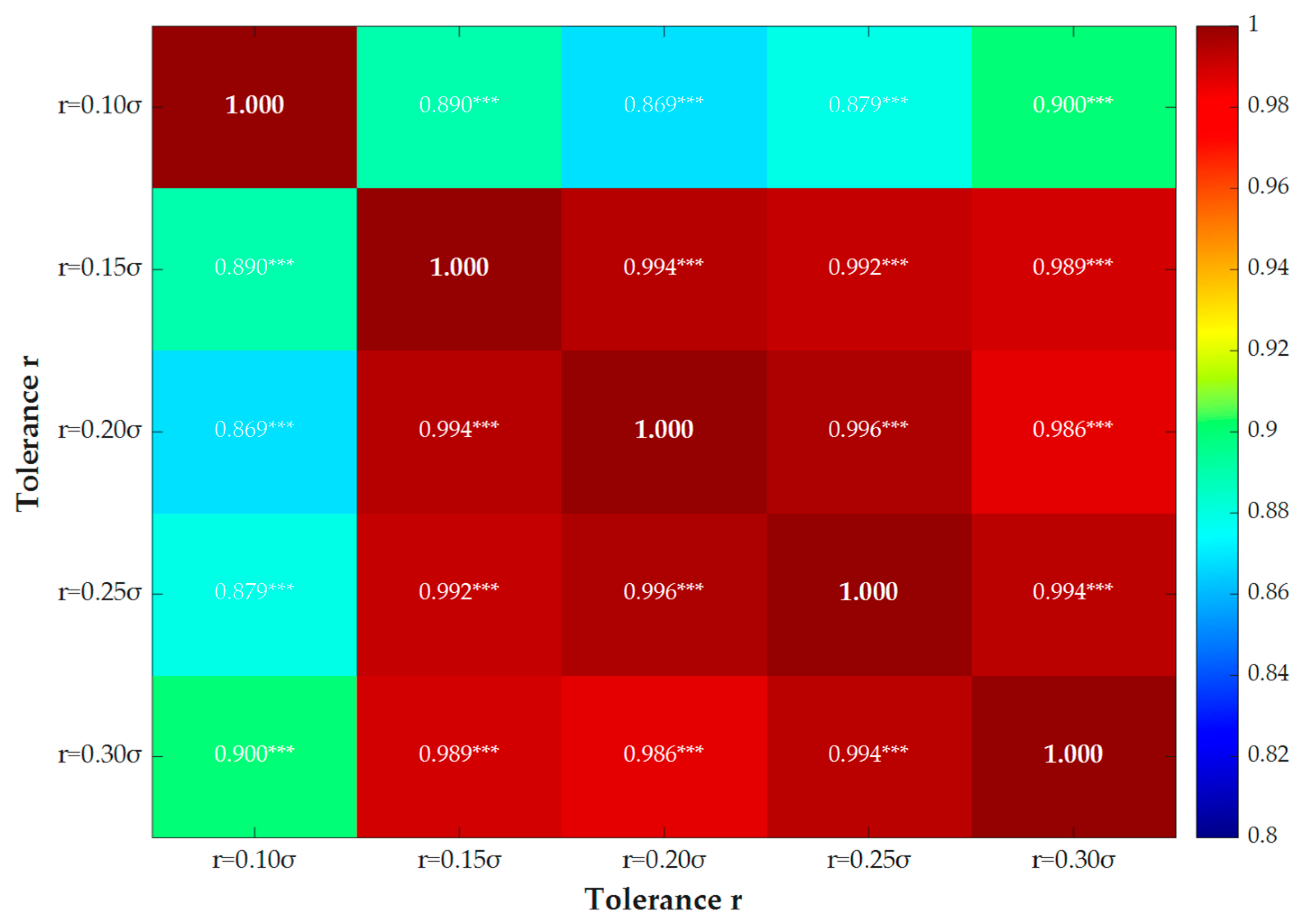
A sensitivity analysis was conducted to verify the robustness of the fitness function to the SampEn tolerance parameter. A total of 500 parameter combinations (α ∈ [2000, 10,000]; K ∈ [2, 16]) were randomly sampled, and the complete fitness value was computed with five tolerance coefficients: r = 0.10, 0.15, 0.20, 0.25, and 0.30 times the standard deviation of each IMF. Figure 3 presents the Spearman rank correlation matrix. The correlation between r = 0.20 and its immediate neighbors (r = 0.15 and r = 0.25) exceeds 0.99 (p < 0.001), and even at r = 0.30, the correlation remains above 0.98. These results confirm that the optimization landscape is highly stable across the range [0.15, 0.25], validating r = 0.20 × std(u_k) as a robust default tolerance coefficient.

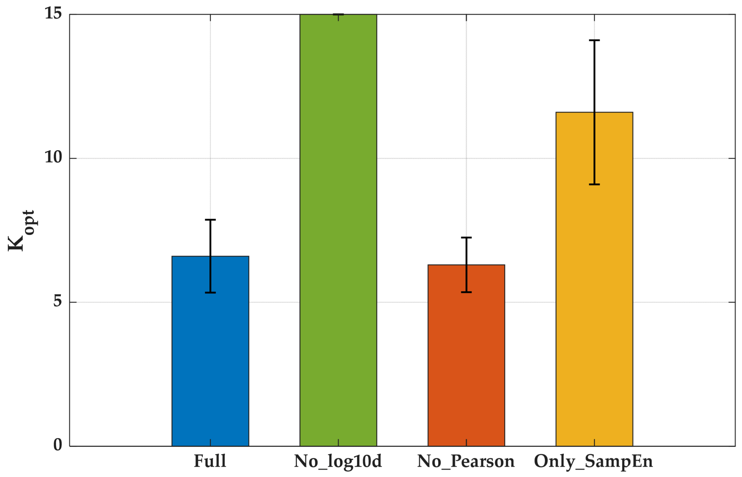
An ablation study was performed to verify the contribution of each component in the fitness function (Equations (18) and (19)). Four variants were tested: (1) Full; (2) No log₁₀(d); (3) No Pearson; and (4) Only SampEn. Each variant was used as the fitness function in SSA-VMD optimization on the measured signal, repeated 10 times. As shown in Figure 4, the full variant yields K_opt = 6.6 ± 1.3, consistent with the physical composition of the bucket runner signal. In contrast, removing log₁₀(d) causes the optimizer to consistently select K = 15 (the upper bound), indicating over-decomposition driven by the absence of convergence cost penalty. Using SampEn alone similarly inflates K_opt to 11.6 ± 2.5. The No Pearson variant produces a K_opt comparable to Full (6.3 ± 0.9), suggesting that Pearson correlation primarily serves as a refinement term rather than a dominant driver. These results demonstrate that the multiplicative combination of all three terms is necessary to guide the optimizer toward physically meaningful decomposition.

2.4.3. Parameter Optimization Process (Parameter Initialization and Search)

Step 1: Initialize the algorithm parameters. The population size is set to 10, the maximum number of iterations is 50, and the initial population is randomly generated. Each individual corresponds to a group (K, α), where K takes integers randomly in [2, 16] and α takes real numbers randomly in [2000, 10,000].

Step 2: For each individual in the population, the K value is rounded and rounded, and the rounded (K, α) performs VMD decomposition on the original signal to obtain K IMF components.

Step 3: Calculate the comprehensive evaluation index as the fitness of the individual according to Equations (12)–(19).

Step 4: Update the population according to the location update rules of the corresponding optimization algorithm.

Step 5: Determine whether the termination condition is satisfied. If the maximum number of iterations is reached, the iteration is stopped; if the variation in the global optimal fitness of 10 consecutive generations is less than 10⁻⁶, it is judged to be convergent, and the iteration is terminated in advance. Early convergence termination not only saves computing resources but also makes the stopping conditions of the algorithm more rigorous.

Step 6: Output the parameter combination (K_opt, α_opt) corresponding to the global optimal individual, where K_opt takes the integer value after the last rounding and performs the final VMD decomposition on the original signal with this parameter.

The four algorithms use a unified population size and number of iterations, and the fitness function and parameter search range are completely consistent to ensure the fairness of the comparison experiment.

2.5. Experimental Verification Scheme and Evaluation Index

This chapter sets up an evaluation index system around the decomposition quality, which is used to horizontally compare the decomposition effects of four optimized VMD methods and traditional empirical parameter VMD. The fitness function in the optimization stage was defined in Section 2.4.2. This chapter is no longer repeated, and only the evaluation scheme is constructed from the dimension of the decomposition effect.

Parameter Optimization Process

In order to comprehensively compare the decomposition effects of the four optimized VMD methods and the traditional empirical parameter VMD, this paper compares and analyzes the three dimensions of fitness curve, time–frequency decomposition effect and eight performance indicators. The eight performance indicators are as follows: the optimal mode number, optimized penalty factor, false mode number, over-decomposition score, under-decomposition score, under-decomposition proportion, residual energy proportion, and computation time. Among them, over-decomposition and under-decomposition are quantitatively evaluated by an independent deduction system. All modal rationality judgments are carried out after eliminating false modes, so as to avoid the interference of meaningless components on the evaluation results.

• Fitness curve

Taking the number of iterations as the abscissa and the global optimal fitness value of the population as the ordinate, the fitness curves of each optimization algorithm are drawn. The faster the curve decreases, the higher the optimization efficiency of the algorithm is. The lower the fitness value after convergence, the better the decomposition quality corresponding to the parameter combination searched by the algorithm.

2.

Residual energy ratio

After VMD decomposition, the residual signal that is not captured by each mode is

$$r\left(t\right)=f\left(t\right)-{\displaystyle \sum _{k=1}^K{u}_k\left(t\right)}$$

(20)

The residual energy ratio is defined as

$${\eta }_r={\displaystyle \frac{{\displaystyle {\sum }_{t=1}^N{r}^2\left(t\right)}}{{\displaystyle {\sum }_{t=1}^N{f}^2\left(t\right)}}}\times 100\%$$

(21)

The smaller the η_r is, the more complete the acquisition of the original signal energy by the modal component is, and the higher the decomposition fidelity is.

3.

The number of optimal modes and the number of false modes

The optimal mode number K_opt is the final decomposition order of each method. Combined with the physical composition of the bucket runner signal, it can be preliminarily judged whether the mode division is reasonable.

Among the IMF components obtained by decomposition, some low-energy components have no clear physical meaning, and most of them are redundant components or noise generated by over-decomposition. In this paper, the proportion of component energy is used as the main criterion of false mode, supplemented by a frequency-domain spectrum peak test. The specific rules are as follows.

The energy ratio of the kth IMF component is defined as

$${\eta }_k={\displaystyle \frac{{\displaystyle {\sum }_{t=1}^N{u}_k^2\left(t\right)}}{{\displaystyle {\sum }_{t=1}^N{f}^2\left(t\right)}}}\times 100\%$$

(22)

Main criterion: If η_k < 0.3%, it is preliminarily judged as a false modal candidate. The selection of the threshold is based on the energy distribution of each redundant component after multiple sets of VMD over-decomposition experiments on the bucket runner signal. The upper-bound empirical value of the redundant component energy is 0.3%, and the components below this threshold have no identifiable physical characteristics in the time domain and frequency domain. The empirical validation of this threshold using the constructed signal with the known ground truth is presented in Section 3.1.5.

Auxiliary criterion: Further check the spectrum of the candidate components that meet the main criterion. If there is no obvious narrowband spectral peak in the frequency domain, it is confirmed as a false mode.

The total number of false modes is K_spurious, and the number of effective modes after removal is

$$K_{\mathrm{eff}}=K_{\mathrm{opt}}-K_{\mathrm{spurious}}$$

(23)

4.

Evaluation of over-decomposition degree

Over-decomposition refers to the phenomenon where the number of modes is too large, and the same physical component is divided into multiple spectral adjacent modes. In this paper, the over-decomposition is determined by the modal separation index, which combines the center frequency difference of adjacent modes with the respective 3 dB bandwidth to quantify the spectral overlap.

5.

Calculation of 3 dB bandwidth

For each IMF component, the spectral peak A_max and its corresponding frequency f_p are located in the frequency domain, and the difference between the left and right frequency points at the peak drop of 3 dB (i.e., the amplitude drop to A_max/√2) is used as the 3 dB bandwidth:

$$BW=f_{\mathrm{right}}-f_{\mathrm{left}}$$

(24)

where f_right and f_left are the frequencies at which the left and right sides of the spectrum peak are lower than the half-power point for the first time, respectively, and are accurately calculated by linear interpolation.

6.

Modal separation calculation

Firstly, the spectrum analysis of the original signal is performed, and the dominant frequency f_peak corresponding to the maximum amplitude of the spectrum is extracted to set the percentage threshold λ₁. λ₁ times the dominant frequency is used as the critical interval for the over-decomposition determination. According to the pre-processing experimental results, this paper takes λ₁ = 0.25 (i.e., 25% of the dominant frequency).

The effective IMFs after eliminating the spurious modes are sorted according to the center frequency from small to large, and the relative frequency separation degree of any ith and jth modes is calculated only within the effective mode, which does not involve the comparison with the residual or out-of-band components:

$${\mathrm{sep}}_{ij}={\displaystyle \frac{2\left|f_i-f_j\right|}{B{W}_i+B{W}_j}}$$

(25)

where f_i and f_j are the central frequencies of the two modes, respectively.

If sep_ij ≥ λ₁∙f_peak, it shows that the frequency interval between the two modes is sufficient, and there is no over-decomposition; if sep_ij ≤ λ₁∙f_peak, the two modal frequencies are close to each other, which is determined to be an over-decomposition event.

7.

Over-decomposition quantitative score

The deduction system is adopted: the initial score is R_over, 1 point is deducted for each over-decomposition event, and the final score is recorded as S_over:

$$S_{\mathrm{over}}=R_{\mathrm{over}}-N_{\mathrm{over}}$$

(26)

where N_over is the number of modal pairs satisfying sep_ij ≤ λ₁∙f_peak, R_over is a positive integer, and 10 is taken in this paper. The higher S_over is, the lighter the degree of over-decomposition is.

8.

Evaluation of under-decomposition degree

Under-decomposition refers to the phenomenon where the number of modes is too small and multiple independent physical components are mixed in the same mode. In this paper, the forced quadratic decomposition method is used to determine the under-decomposition. The method is as follows.

For each valid IMF component, the second VMD decomposition is enforced, and the number of sub-modes K₂ = 2 is fixed. The penalty factor α₂ of the second decomposition is 1.2 times the optimal value α_opt of the first decomposition. The sensitivity analysis and empirical justification for this multiplier are provided in Section 3.1.6.

$${\alpha }_2=1.2\times {\alpha }_{\mathrm{opt}}$$

(27)

The remaining control parameters follow the setting of one decomposition to ensure the consistency of the decomposition bandwidth constraint and the reproducibility of the experiment.

The percentage threshold λ₂ is set, and λ₂ times the maximum amplitude value A’_max of the original IMF spectrum is taken as the amplitude determination threshold. According to the results of preprocessing experiments, this paper takes λ₂ = 0.35 (i.e., 35% of the spectral peak), which can effectively distinguish the real physical components from the decomposed noise. If the maximum amplitude of the two sub-mode spectra of the secondary decomposition is greater than λ₂∙A’_max, it indicates that the original mode still contains two separable independent components, and it is determined that the mode has under-decomposition.

The deduction system is adopted: the initial score is R_under, 1 point is deducted for each under-decomposition event, and the final score is recorded as S_under:

$$S_{\mathrm{under}}=R_{\mathrm{under}}-N_{\mathrm{under}}$$

(28)

where N_under is the number of under-decomposed modes, R_under is a positive integer, and 10 is taken in this paper. The higher the S_under, the lighter the degree of under-decomposition.

At the same time, the proportion of under-decomposition is defined as

$${\eta }_{\mathrm{under}}={\displaystyle \frac{N_{\mathrm{under}}}{K_{\mathrm{eff}}}}\times 100\%$$

(29)

This index quantifies the proportion of under-decomposition under each method.

S_over and S_under are independent of each other, and the rationality of modal division is evaluated from the two opposite dimensions of ‘excessive separation’ and ‘insufficient separation’, respectively, which jointly reflect the matching degree between parameter selection and signal characteristics. The empirical validation of this scoring system using the constructed signal is presented in Section 3.1.7.

3. Results and Discussion

3.1. Structural Signal Analysis

3.1.1. Overview of Artificially Constructed Signal

In order to test the modal separation ability, the effectiveness of parameter optimization, and the rationality of the over-decomposition and under-decomposition evaluation indexes of the four optimized VMD methods, a complex artificial signal is constructed in this paper. The signal expression is

$$\begin{array}{l}f\left(t\right)=0.45e^{-32t_{\mathrm{mod}}}\cos \left(280\pi t_{\mathrm{mod}}\right)\left[\cos \left(32\pi t\right)+2.8\right]\\ +0.06e^{-12t_{\mathrm{mod}}}\cos \left(180\pi t_{\mathrm{mod}}\right)\cos \left(32\pi t\right)+0.03e^{-6t}\cos \left(80\pi t\right)\\ +0.05\cos \left(64\pi t_{\mathrm{mod}}\right)\cos \left(320\pi t\right)+0.04\sin \left(48\pi t\right)\cos \left(440\pi t\right)\\ +0.28\cos \left(320\pi t\right)+0.15\cos \left(440\pi t\right)+0.12\cos \left(120\pi t\right)\\ +0.02\cos \left(96\pi t\right)+0.08n\left(t\right)\end{array}$$

(30)

The periodic modulation time variable is defined as

$$t_{\mathrm{mod}}=d\left(t,0.1\right)$$

(31)

The structural signal is composed of 10 components, including nine deterministic components and one Gaussian white noise term, covering six main frequency centers. The signal has four kinds of non-stationary characteristics: periodic attenuation impact, amplitude modulation–frequency modulation coupling, same-frequency superposition and strong and weak coexistence. The time-domain impact characteristics and frequency-domain multi-component coupling characteristics of the non-stationary signal of bucket runners are simulated. The specific parameters of each component are shown in

Table 1. Construct the parameters of each component of the signal.

Number of Terms	Amplitude	Center Frequency (Hz)	Type
1	0.45	140	Periodic attenuation impact
2	0.06	90	Amplitude-modulated–frequency-modulated component
3	0.03	40	Steady-state attenuation harmonics
4	0.05	160	Amplitude-modulated–frequency-modulated component
5	0.04	220	Amplitude modulation component
6	0.28	160	Stationary harmonic
7	0.15	220	Stationary harmonic
8	0.12	60	Stationary harmonic
9	0.02	48	Stationary harmonic
10	0.08	-	Gaussian white noise

The sampling parameters of the simulation signal are set as follows: sampling frequency f_s = 1000 Hz, time interval ∆t = 0.001 s, and total sampling points n = 1200.

.

3.1.2. Analysis of Fitness Curve (Convergence Analysis of Optimization Algorithms)

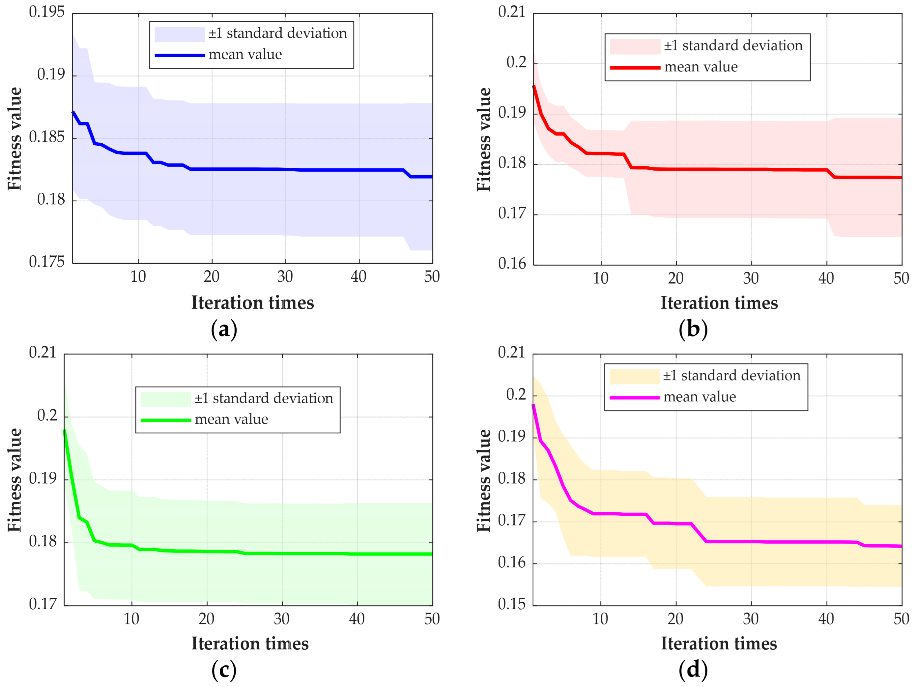
Figure 5a–d present the fitness convergence curves of four algorithms averaged over 30 independent runs, with shaded bands indicating ±1 standard deviation. WOA-VMD converges most rapidly by the 25th iteration, while PSO-VMD and GWO-VMD stabilize by the 41st and 45th iterations, respectively. SSA-VMD converges by the 46th iteration and demonstrates the narrowest variance band (std = 0.0059), reflecting the most consistent search behavior among the four algorithms.

In terms of mean fitness values, GWO (0.1642) achieves the lowest, followed by PSO (0.1774), WOA (0.1782), and SSA (0.1819). However, Wilcoxon rank-sum tests confirm that no statistically significant difference exists between SSA and the other three algorithms (p > 0.05 for all pairwise comparisons). This indicates that the four algorithms achieve comparable optimization performance on the constructed signal.

3.1.3. Time–Frequency Diagram Analysis (Time–Frequency Diagram Analysis of the Structural Signal)

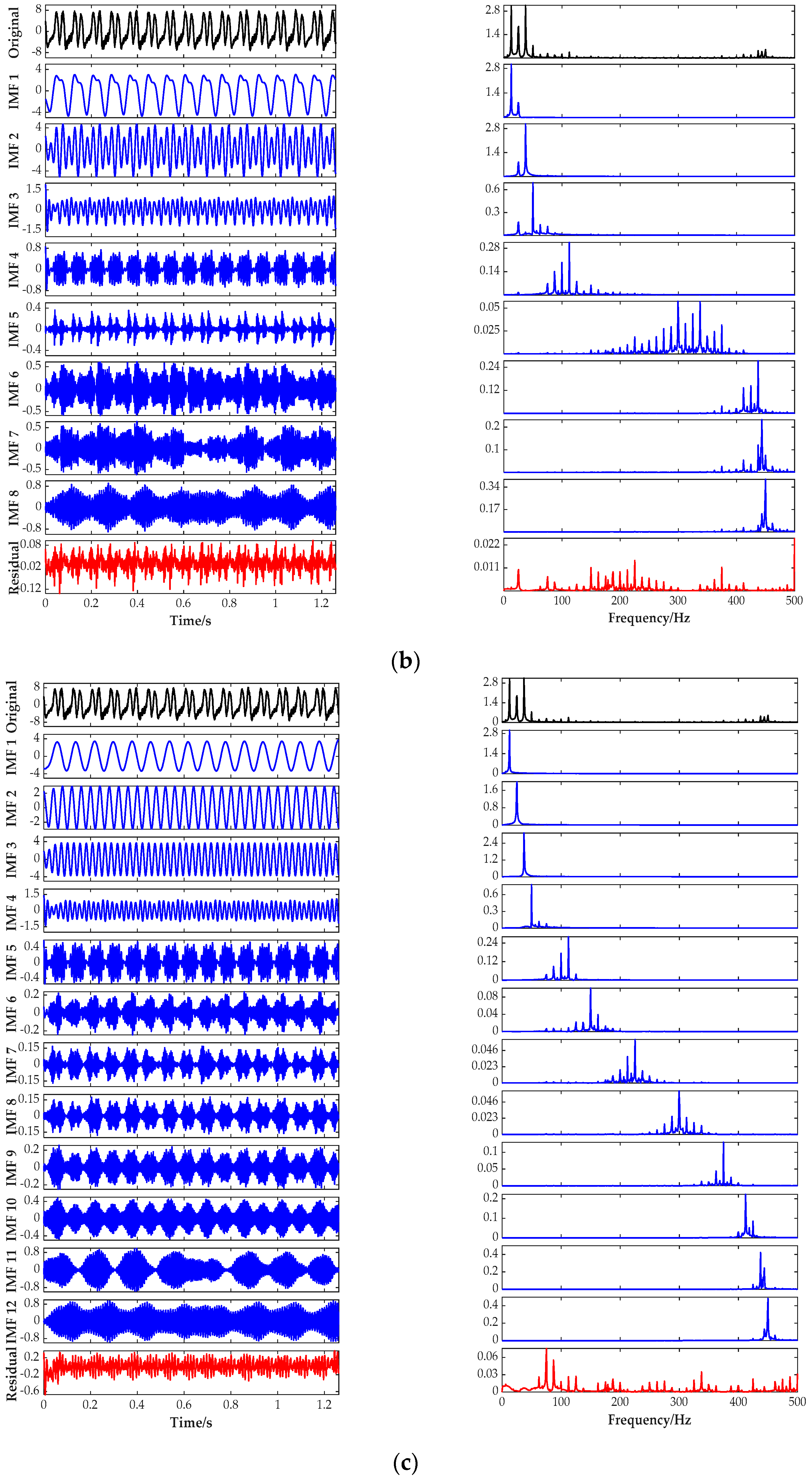
Figure 6a–e give the time domain decomposition results and corresponding spectra of the five algorithms for the constructed signal. It can be seen from the figure that there are obvious multi-component aliasing characteristics in the IMF waveforms of the traditional empirical parameter VMD (K_opt = 4). The IMF1 spectrum shows a broadband distribution, covering the range of 40–120 Hz, indicating that multiple frequency components are compressed in the same mode. The envelope structure is irregular, and K_opt = 4 is far from enough to cover the six main frequency centers of the simulation signal.

The number of modes of PSO-VMD (K_opt = 12) is large, and some IMFs have extremely low amplitude in the time domain, a nearly flat waveform, and no obvious narrowband peak in the spectra, showing redundant component characteristics. At the same time, the waveform morphology of some adjacent effective modes is highly similar, and the spectra overlap, indicating that there is an over-decomposition phenomenon.

Although the number of modes of WOA-VMD (K_opt = 13) and GWO-VMD (K_opt = 14) is high, the waveforms of multiple effective IMFs still contain more than two frequencies of oscillation at the same time. Broadband aliasing can be observed in the spectra, and the components are not completely separated.

In contrast, the effective modal waveforms of SSA-VMD (K_opt = 9) are the purest, and the spectra show a single narrowband peak. The center frequency corresponds to the main frequency center of the simulated signal one by one. The IMF corresponding to the impact attenuation component clearly shows an attenuation envelope structure with a period of 0.1 s, and the characteristic peaks corresponding to the impact frequency in the spectrum are clearly distinguishable, indicating that SSA-VMD has the best separation effect on each physical component. In the decomposition results of SSA-VMD, each component of the test signal presents a single center frequency feature and does not interfere with others. The useful signal component and the noise component are clearly separated. Therefore, in terms of optimizing the VMD parameter combination, SSA-VMD has the best global search effect.

3.1.4. Quantitative Comparison of Decomposition Quality (Quantitative Comparison of Decomposition Quality of the Structural Signal)

Table 2. Performance indicators. (Performance indicators of the structural signal).

Optimistic Algorithm	Kopt	Kspurious	αopt	Sover	Sunder	ηunder	ηr	T (s)
VMD	4	0	2000	10	8	50.00%	7.56%	-
SSA-VMD	9	3	3990	10	8	33.33%	3.78%	123.1
PSO-VMD	12	6	9900	7	9	16.67%	4.65%	432.4
WOA-VMD	13	4	2130	9	4	66.67%	0.55%	260.0
GWO-VMD	14	5	2730	5	6	44.44%	0.67%	258.1

shows the quantitative comparison results of five methods on eight performance indicators.

From the perspective of modal number, SSA-VMD outputs K_opt = 9, which is consistent with the number of nine deterministic components of the signal. After removing three false modes, the effective modal number K_eff = 6, corresponding to six main frequencies; PSO-VMD, WOA-VMD and GWO-VMD all select a higher number of modes, the output K_opt is 12, 13 and 14 respectively, and the number of false modes is six, four and five respectively. The high proportion of false modes indicates that the parameter combination makes VMD split the continuous energy or noise base in the signal into redundant components without physical meaning, and the effectiveness of the decomposition results is reduced. Compared with the other four optimization algorithms, the VMD output K_opt = 4 is significantly lower.

From the perspective of the penalty factor α, VMD adopts the empirical default value of 2000. SSA-VMD selects α_opt = 3990, which is a moderate increase and provides sufficient bandwidth constraint without excessive mode splitting. PSO-VMD selects the highest α_opt = 9900, nearly five times the default value. The excessively large penalty factor forces VMD to adopt an overly narrow bandwidth for each mode, which is the primary reason for the maximum number of six false modes and the severe over-decomposition observed. WOA-VMD and GWO-VMD select α_opt = 2130 and 2730, respectively, both close to the default value, indicating that these two algorithms fail to significantly adjust the bandwidth constraint during optimization, which partly explains their inadequate separation of similar frequency components and severe under-decomposition.

From the perspective of the degree of over-decomposition, the SSA-VMD and VMD scores are both 10 points, and there is no aliasing pair adjacent to the spectrum within the effective mode; The degree of over-decomposition of GWO-VMD is the most serious, with a score of only five points and five over-decomposition events.

From the perspective of the degree of under-decomposition, PSO-VMD has the highest score of 9 points. There is only one under-decomposition event in the effective mode, and the proportion of under-decomposition is the lowest, which is 16.67%. The scores of SSA-VMD and VMD are both eight points, and there are two under-decomposition events. However, the under-decomposition ratios of SSA-VMD and VMD are different, at 33.33% and 50% respectively, which is due to the difference in the number of effective modes. WOA-VMD has the most serious under-decomposition degree, and the under-decomposition score is only four points. There are six under-decomposition events, and the proportion of under-decomposition is as high as 66.67%, indicating that the parameter combination fails to make VMD effectively separate similar frequency components.

From the perspective of residual energy ratio, the residual energy ratios of WOA-VMD and GWO-VMD are relatively low, at 0.55% and 0.67%, respectively. However, this is due to the high number of decomposition modes, which leads to a low energy ratio and cannot represent high decomposition quality. The residual energy ratio of SSA-VMD is 3.78%, which achieves a good balance between decomposition fidelity and resolution.

From the perspective of computational efficiency, SSA-VMD achieves the shortest optimization time of T = 123.1 s, which is attributed to the strong global search capability and fast convergence of the sparrow search algorithm. WOA-VMD and GWO-VMD require 260 s and 258.1 s, respectively, approximately four times that of SSA-VMD, reflecting their relatively slower convergence in the multi-parameter optimization landscape. PSO-VMD consumes the longest time of T = 432.4 s, nearly seven times that of SSA-VMD, which is related to its tendency to be trapped in local optima during the search process, requiring more iterations to converge. Since VMD uses fixed empirical parameters without an optimization process, no computation time is recorded.

In summary, the traditional empirical parameter VMD is limited by the subjectivity of manual parameter selection and prone to under-decomposition. PSO-VMD, with the highest number of false modes, an excessively large penalty factor (α_opt = 9900), and the longest computation time (432.4 s), results in a large number of redundant modes and obvious over-decomposition, although the separation effect within the effective mode is the best. WOA-VMD has the highest fidelity but the worst separation, and its moderate computation time (260 s) does not translate into effective parameter optimization. GWO-VMD exhibits coexisting over-decomposition and under-decomposition with a comparable computational cost (258.1 s). SSA-VMD demonstrates the best comprehensive performance across all eight performance indicators: the output K_opt = 9 matches the signal’s deterministic components, the penalty factor α_opt = 3990 achieves a well-balanced bandwidth constraint, the residual energy ratio of 3.78% maintains a good trade-off between fidelity and resolution, and with the shortest computation time of only 123.1 s, it provides the clearest correspondence between the purity of the time-domain waveform and the physical composition. The effectiveness of SSA in the adaptive optimization of VMD parameters is fully verified, which provides a methodological basis for the subsequent decomposition experiment of actual bucket runner signals.

Notably, SSA-VMD achieves the best decomposition quality (the fewest spurious modes; Sover = 10) despite not having the lowest fitness, indicating that fitness alone is insufficient to evaluate optimization performance and validating the necessity of the multi-indicator evaluation system.

3.1.5. Validation of the Spurious Mode Identification Threshold

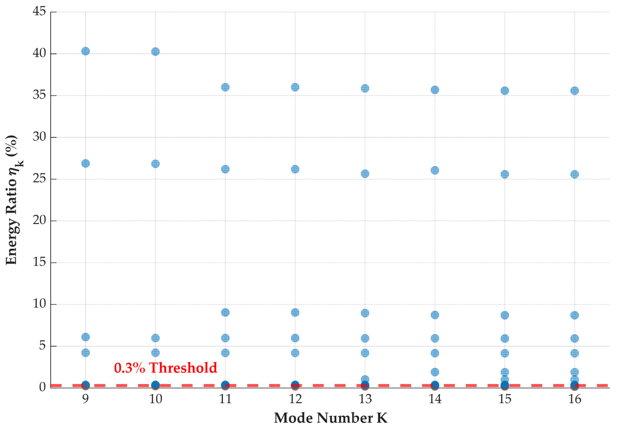
To validate the 0.3% energy threshold, the constructed signal was decomposed using VMD with a K ranging from 9 to 16 at a fixed penalty factor α = 4000, producing a series of controlled over-decomposition scenarios. Since the signal contains nine deterministic components (Table 1), the spurious modes introduced by over-decomposition provide labeled ground truth for threshold evaluation.

As shown in

Table 3. Validation results of the 0.3% energy threshold across different over-decomposition levels.

K	ηk < 0.3%	ηk ≥ 0.3%	False Maximum ηk (%)	Real Minimum ηk (%)	Safety Clearance (%)
9	3	6	0.2520	0.3671	0.1150
10	3	7	0.2536	0.3460	0.0925
11	3	8	0.2715	0.3434	0.0719
12	4	8	0.2460	0.3422	0.0962
13	4	9	0.2473	0.3364	0.0891
14	5	9	0.2422	0.3048	0.0626
15	5	10	0.2414	0.3034	0.0620
16	6	10	0.2370	0.3015	0.0645

, the maximum η_k among spurious modes (0.254%) remains consistently below 0.3%, while the minimum η_k among meaningful components (0.302%) stays above 0.3%, with a safety gap of at least 0.048% across all tested K values. Figure 7 presents the energy distribution across different K values, where the bimodal clustering of η_k above and below the 0.3% line confirms the threshold’s effectiveness with zero misclassification.

3.1.6. Verification of the Multiplier in the Under-Decomposition Test

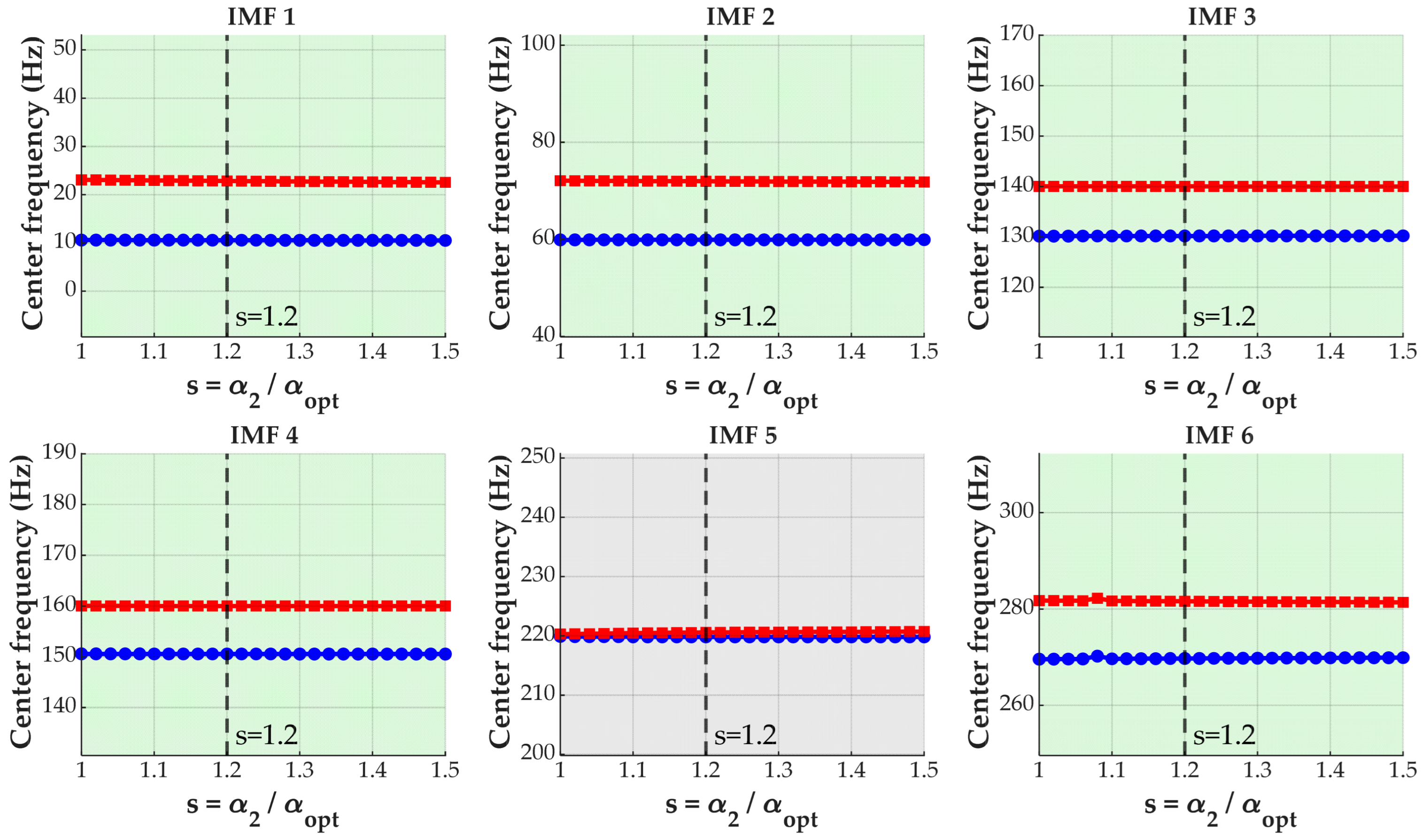
The under-decomposition test applies a secondary VMD decomposition with penalty factor α₂ = 1.2 × α_opt to each valid IMF. To verify that this multiplier produces genuine frequency separation without inducing artificial spectral splitting, a sensitivity analysis was conducted by varying s = α₂/α_opt from 1.0 to 1.5 in steps of 0.02. For each valid IMF, two sub-modes were extracted, and their frequency separation was monitored. Adaptive thresholds of 5% and 20% of the signal main frequency (140.0 Hz) were adopted for the no-separation boundary (7.0 Hz) and over-separation boundary (28.0 Hz), respectively.

The results are summarized in

Table 4. Separation degree of sub-modes at s = 1.2 for each valid IMF component.

IMF	Center Frequency (Hz)	S = 1.2 Degree of Separation (Hz)	Decision
1	16.42	12.3	Effective segregation
2	60.53	12.1	Effective segregation
3	138.89	9.8	Effective segregation
4	159.37	9.5	Effective segregation
5	219.87	0.8	Single-component mode
6	276.92	11.9	Effective segregation

and Figure 8. Five out of six valid IMFs (IMF1, IMF2, IMF3, IMF4, and IMF6) exhibit stable frequency separation in the range of 9.5–12.3 Hz at s = 1.2, all falling within the effective interval [7.0, 28.0] Hz. These separations remain well below the over-separation threshold across the entire range s ∈ [1.0, 1.5], confirming that the observed sub-mode splitting is physically meaningful rather than an artifact of the penalty factor. In contrast, IMF5 (center frequency: 219.9 Hz) remains unseparated throughout the test range (separation = 0.8 Hz at s = 1.2), indicating that it is a single-component mode with no hidden sub-components. The multiplier 1.2, therefore, provides a sufficient bandwidth reduction to expose genuinely mixed components while maintaining a robust safety margin against false detections.

3.1.7. Validation of the Decomposition Quality Scoring System

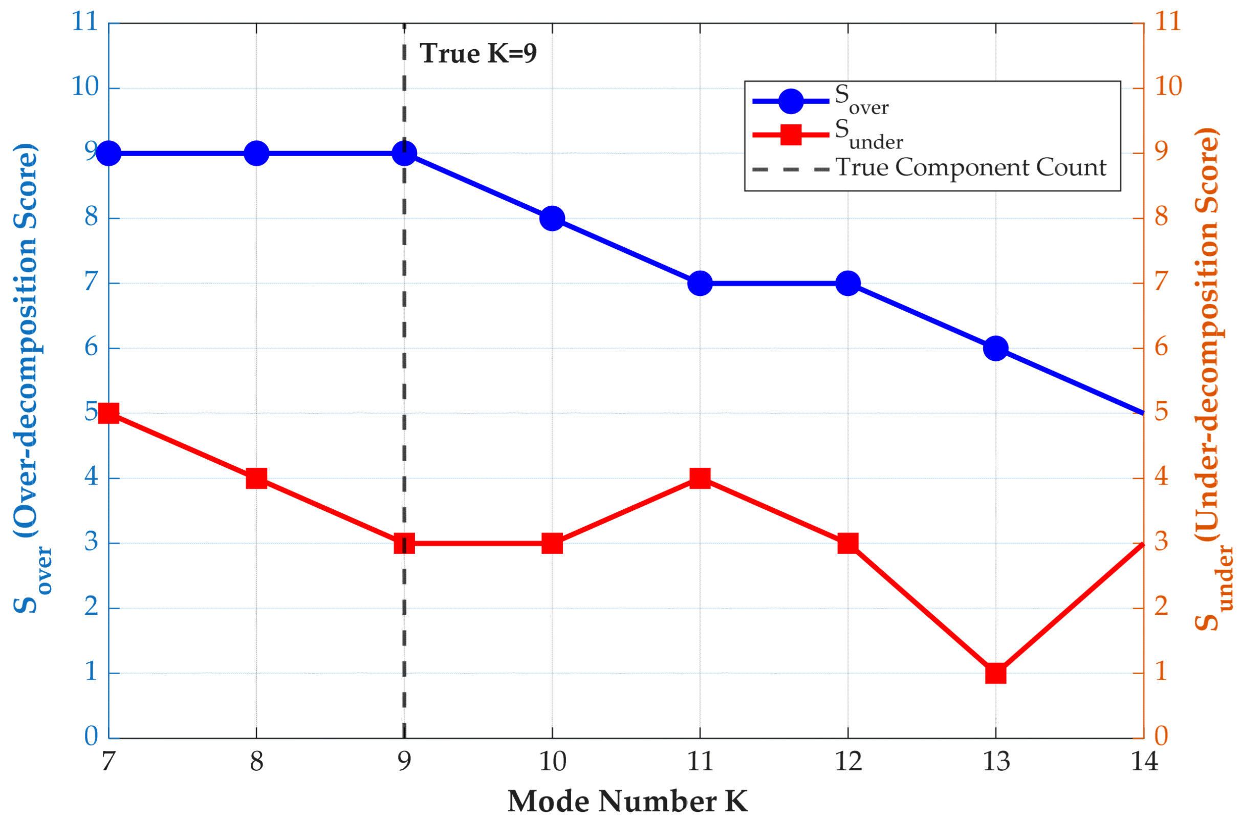
The decomposition quality scoring system was validated using the constructed signal with the known ground truth. VMD was applied with K ranging from 7 to 14. As shown in Figure 9, S_over remains at 9 for K ≤ 9 and decreases progressively for K > 9, correctly identifying the onset of over-decomposition. The consistent N_over = 1 for K ≤ 9 reflects two naturally adjacent frequency components in the constructed signal.

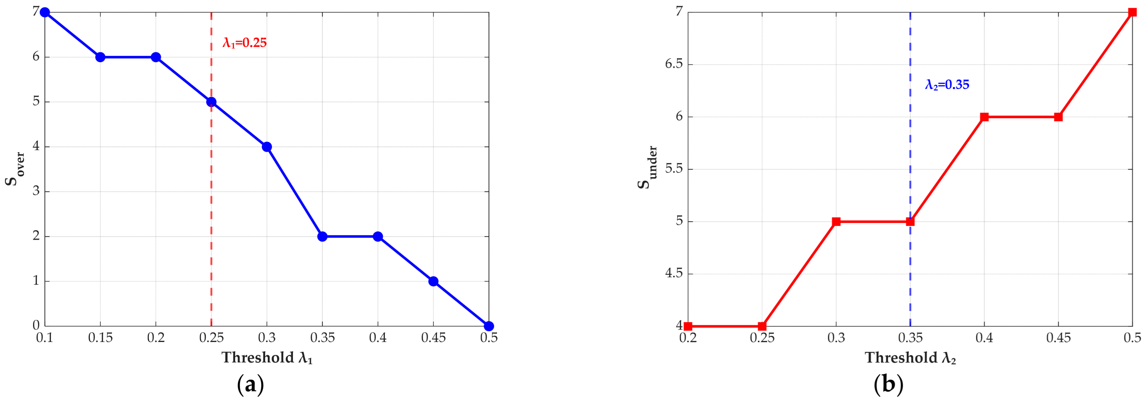
Sensitivity analyses of the threshold parameters (Figure 10) confirm that λ₁ = 0.25 and λ₂ = 0.35 lie within stable regions where small perturbations do not change the scoring results, validating these empirical choices.

3.1.8. Robustness Analysis Under Different Noise Levels

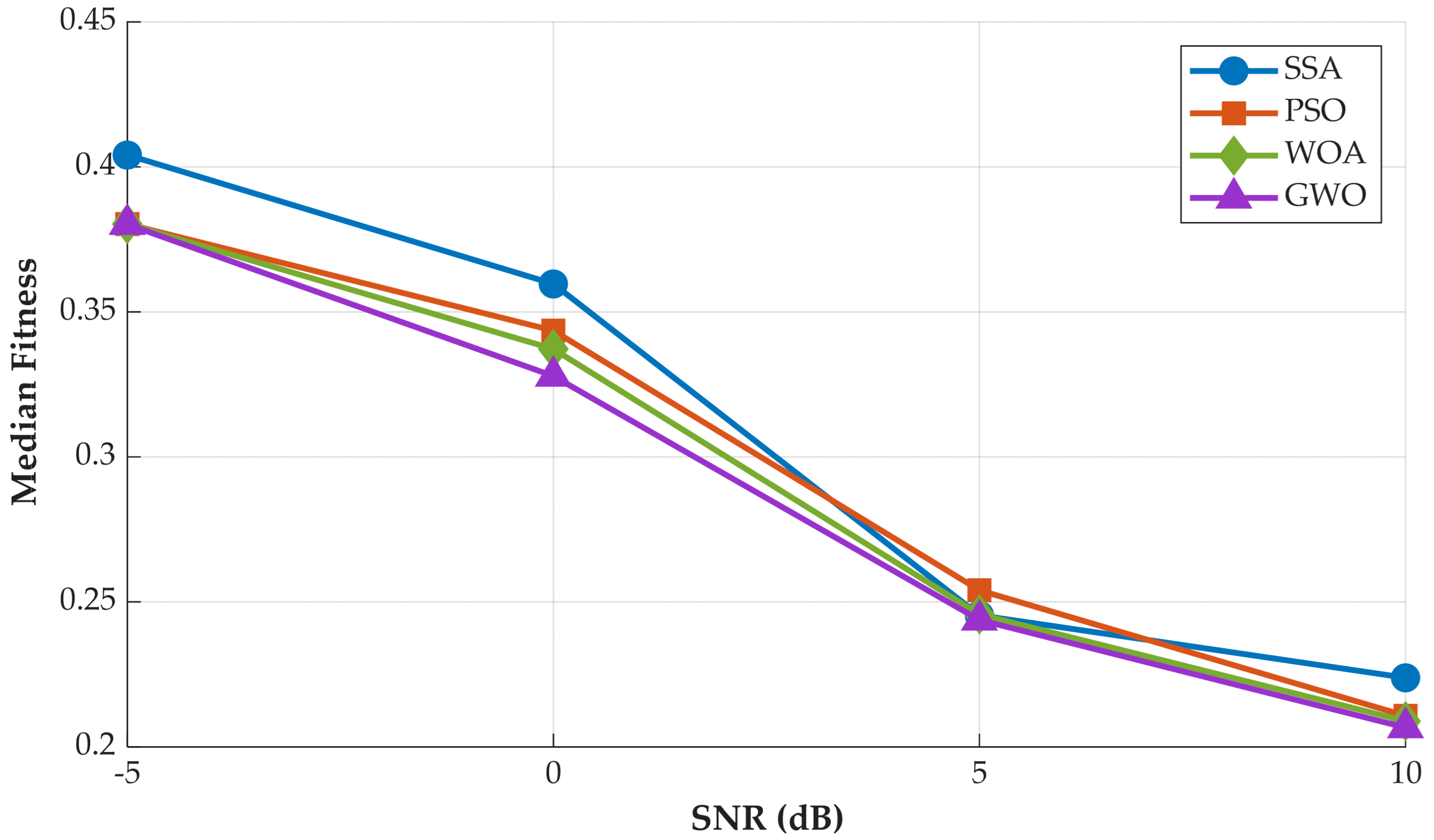
Robustness analysis was conducted by adding Gaussian white noise at four SNR levels (−5, 0, 5, and 10 dB) to the constructed signal. Each algorithm was run 30 times at each SNR level. As shown in

Table 5. Separation degree of sub-modes at s = 1.2 for each valid IMF component. (Fitness values and degradation ratios of different algorithms under different SNR levels.)

Algorithm	SNR = −5 dB	SNR = 0 dB	SNR = 5 dB	SNR = 10 dB	Degradation
SSA	0.4171 ± 0.0583	0.3477 ± 0.0356	0.2713 ± 0.0486	0.2280 ± 0.0304	80.5%
PSO	0.3891 ± 0.0365	0.3359 ± 0.0332	0.2625 ± 0.0334	0.2090 ± 0.0152	80.5%
WOA	0.3888 ± 0.0339	0.3317 ± 0.0347	0.2594 ± 0.0384	0.2071 ± 0.0162	82.0%
GWO	0.3879 ± 0.0341	0.3288 ± 0.0348	0.2555 ± 0.0352	0.2063 ± 0.0168	84.0%

and Figure 11, all four algorithms exhibit increasing fitness values as the SNR decreases, confirming the expected degradation under stronger noise conditions. GWO consistently achieves the lowest fitness across all SNR levels, while SSA shows the highest values. However, SSA demonstrates the most robust performance with the smallest degradation ratio (80.5%), compared with GWO (84.0%). This indicates that SSA’s multi-role exploration mechanism provides more stable optimization behavior under varying noise conditions.

3.2. Measured Signal Decomposition

3.2.1. Overview of Measured Signal

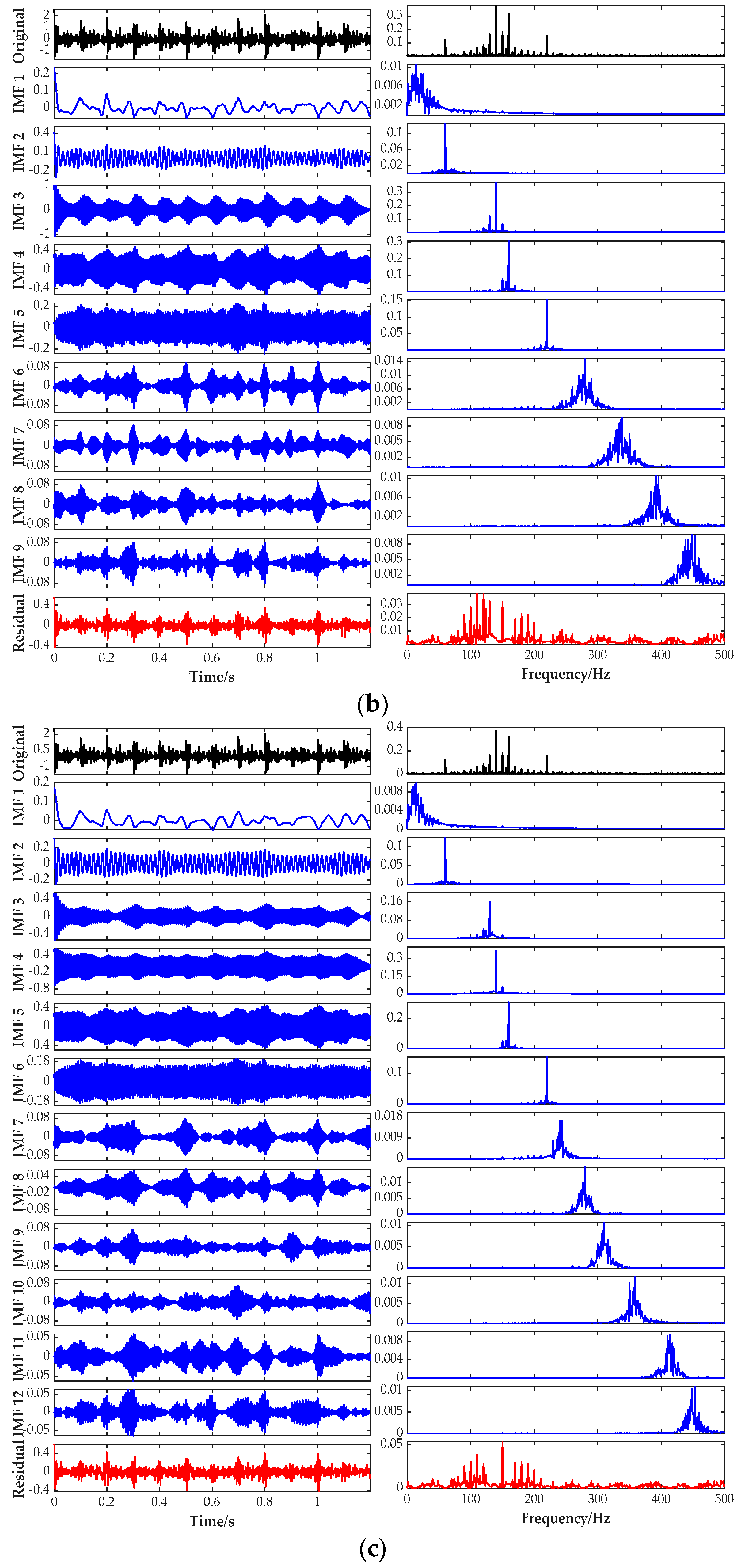
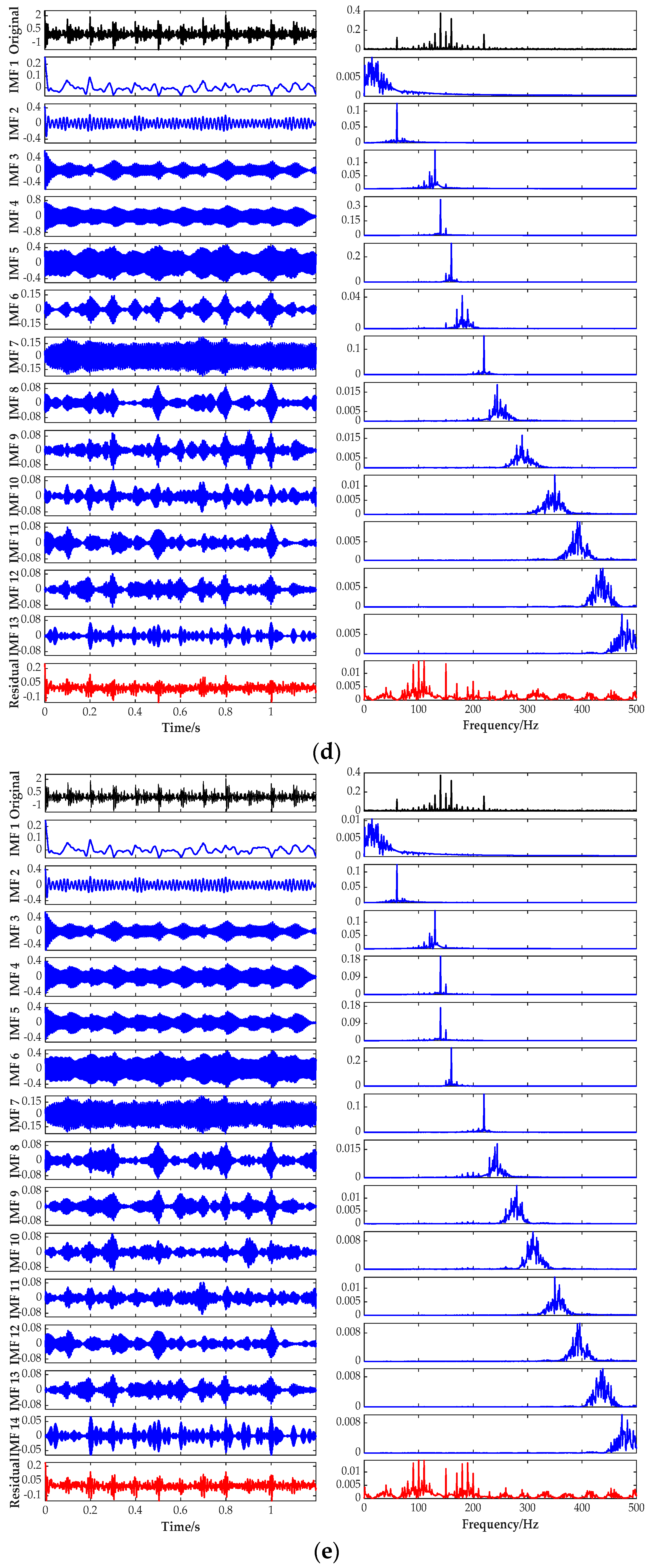
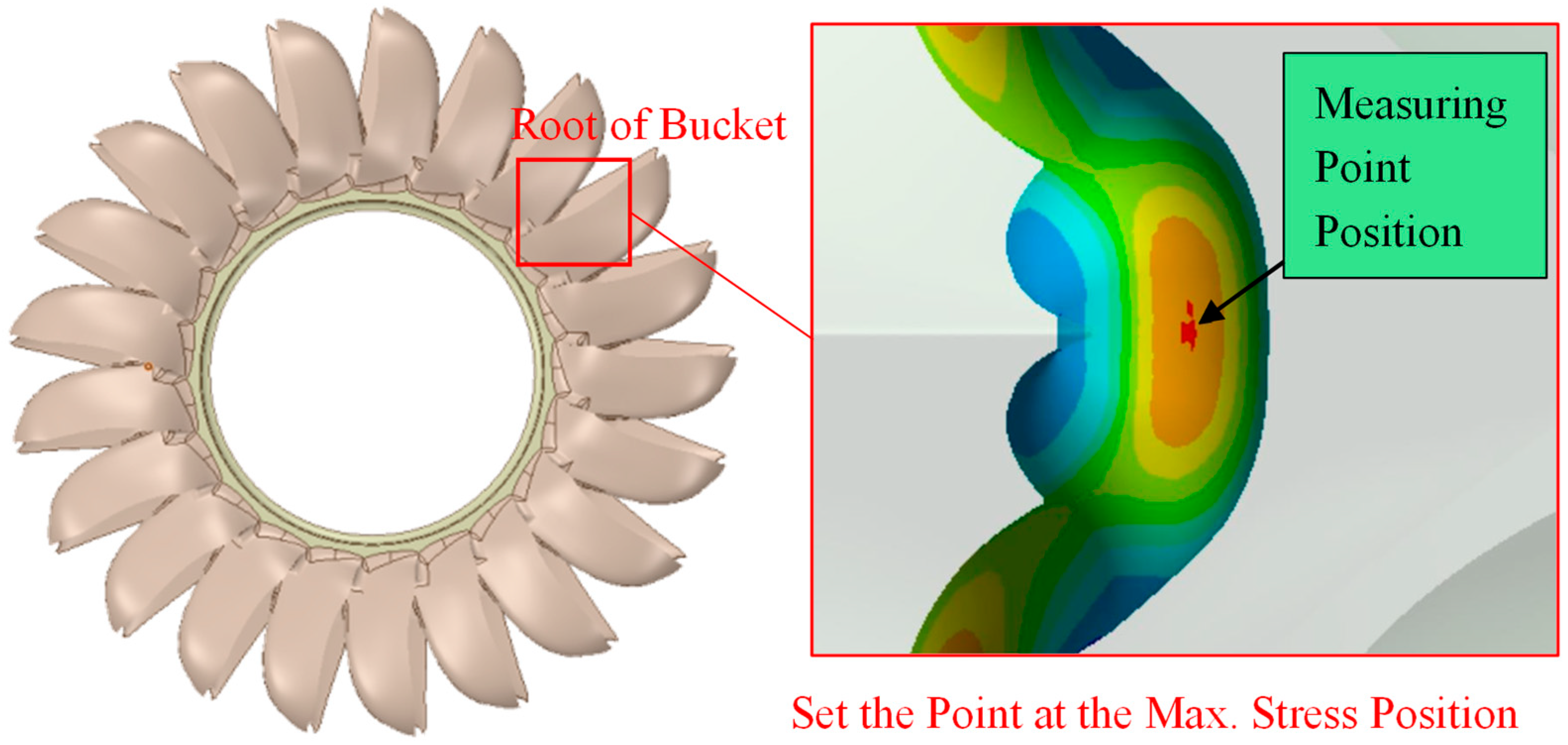
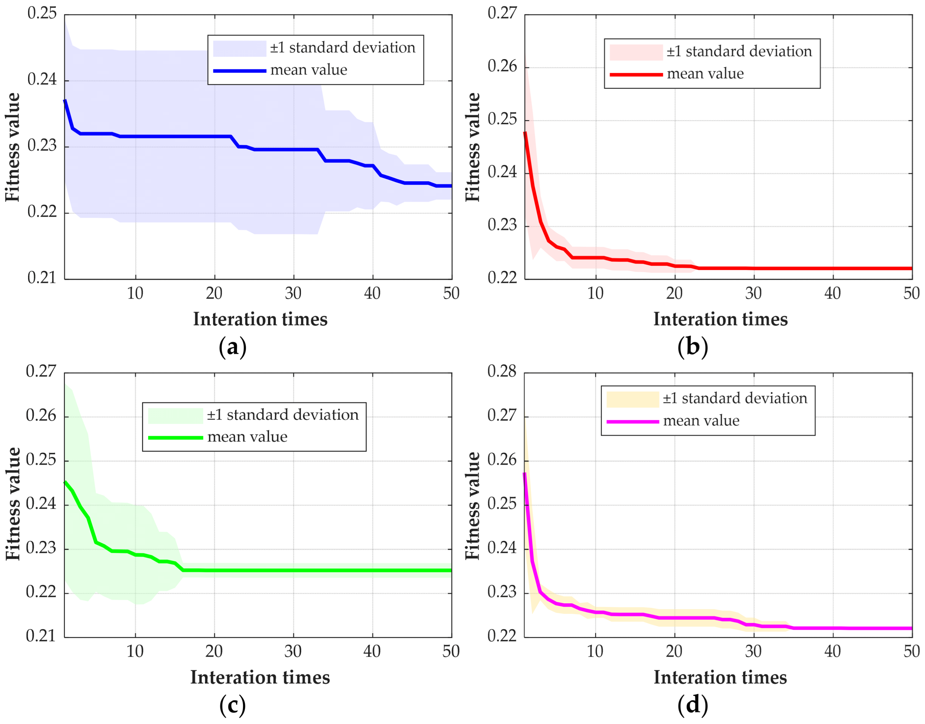
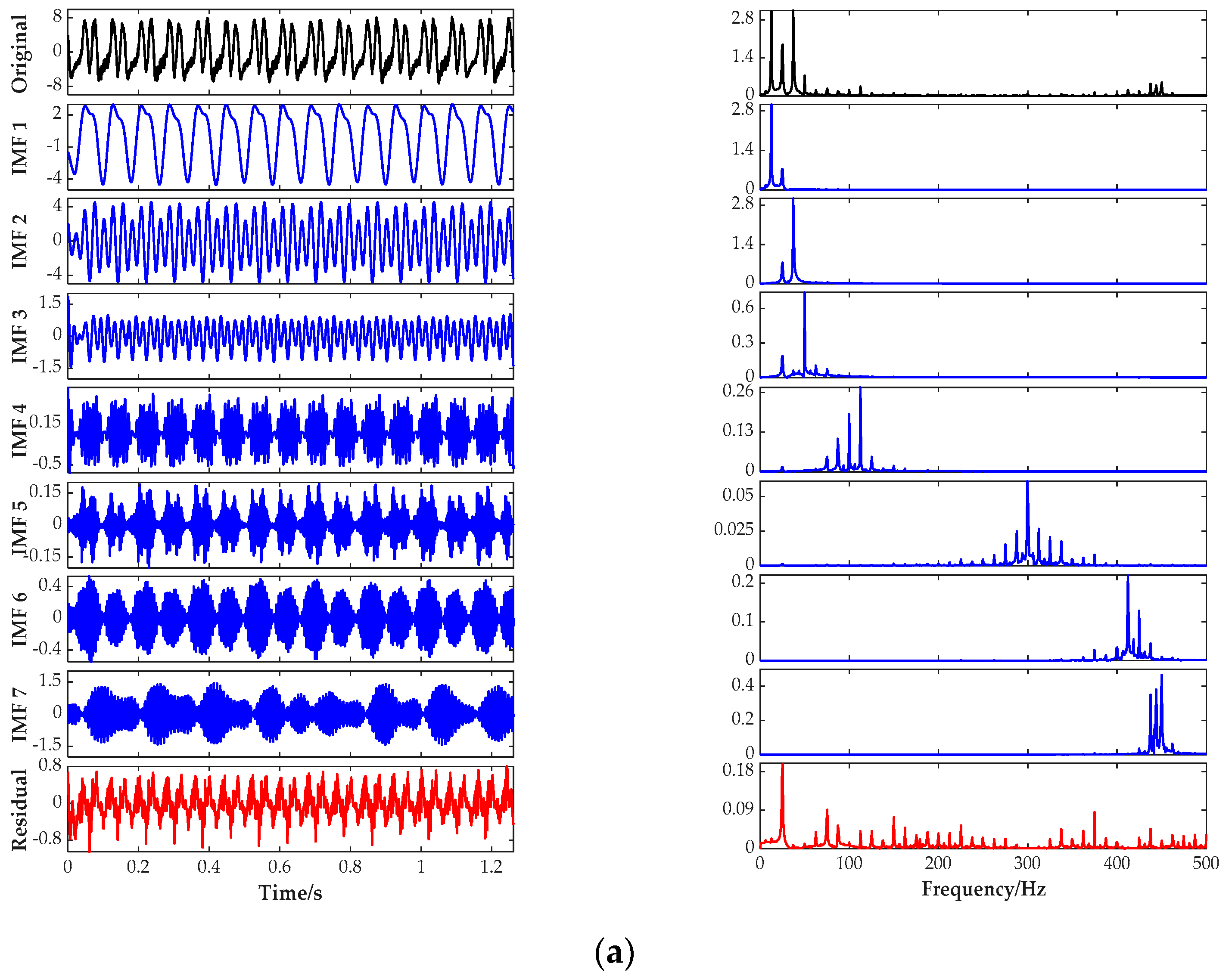
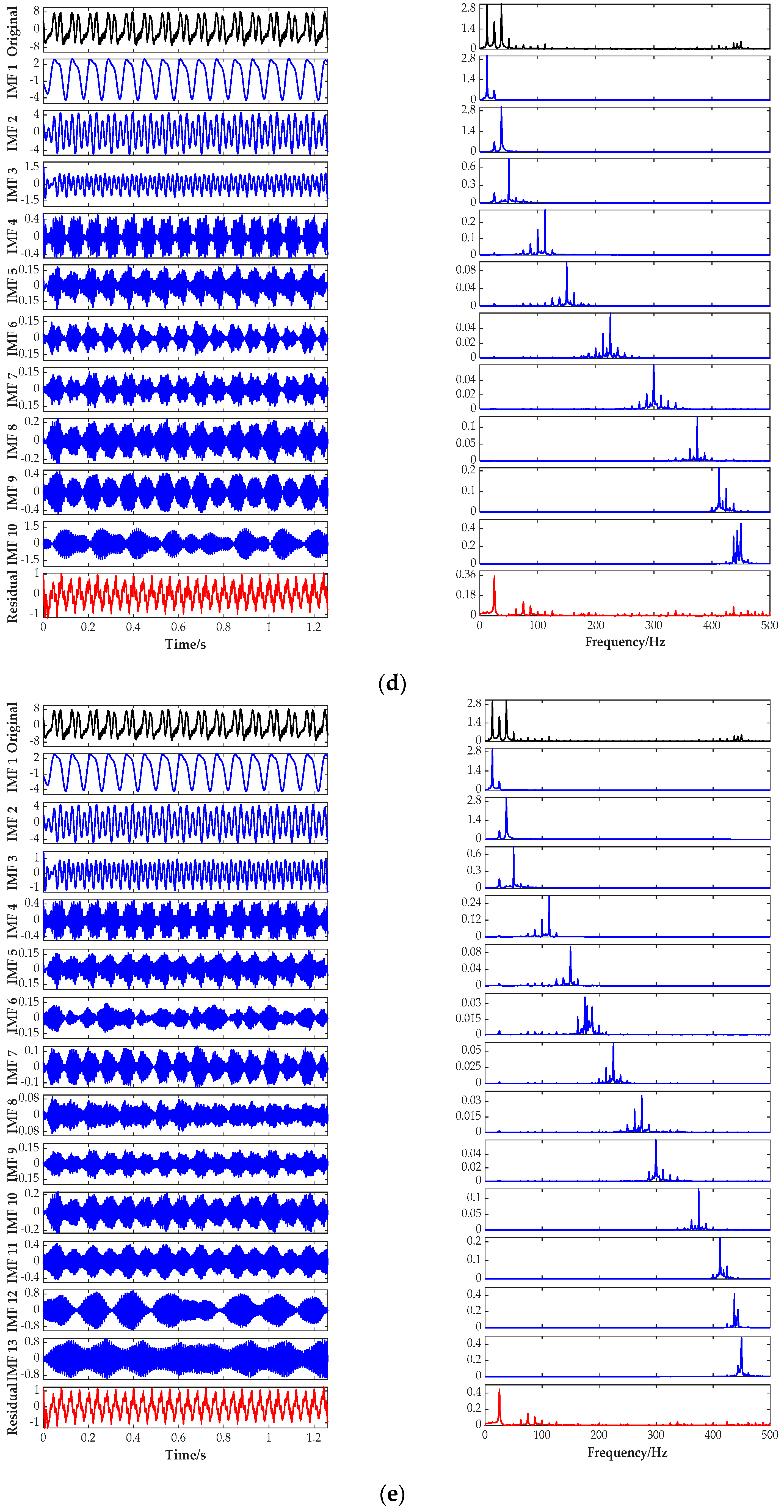
In this example, the stress monitoring data of the 4# bucket of a hydropower station are decomposed and analyzed to verify the effectiveness of the proposed method. The relevant parameters of data acquisition are shown in

Table 6. Data-acquisition-related data.

Rated Speed	Working Condition	Measuring Point Position	Sampling Frequency	Sampling Point
375 r/min	50 MW	The maximum stress point at the root of the bucket	1000 Hz	1260

. The rated speed of the unit is 375 r/min, and the corresponding unit rotation frequency is f_r = 375/60 = 6.25 Hz. The measuring point is located at the maximum stress point at the root of the bucket (as shown in Figure 12), and the measurement method adopts the right-angle strain flower and half-bridge method. During the operation of the bucket turbine, the jet impacts the surface of the bucket at a high speed. Each bucket will produce a transient stress impact when passing through the jet, with the resulting bucket passing frequency. The bucket stress signal contains the transient response of the jet impact, the bucket passing frequency and its harmonic components, as well as the low-frequency modulation and random noise caused by the fluctuation in the working condition, which has typical non-stationary multi-component characteristics. The fitness curves of the four optimization methods are shown in Figure 13. The time-domain diagram and spectrum diagram of different optimization methods of the water bucket stress signal of the unit are shown in Figure 14.

3.2.2. Analysis of Fitness Curve

Figure 13a–d present the fitness convergence curves of four algorithms for the measured signal, averaged over 30 independent runs. PSO-VMD and GWO-VMD converge to identical fitness values (0.2221) with zero variance, suggesting consistent convergence to the same solution. WOA-VMD converges most rapidly by the 16th iteration, while PSO-VMD stabilizes by the 23rd iteration. GWO-VMD requires until the 36th iteration to stabilize. SSA-VMD converges by the 47th iteration with the narrowest variance band (std = 0.0021), demonstrating the most consistent search behavior. Although its mean fitness (0.2241) is slightly higher than PSO/GWO, Wilcoxon rank-sum tests confirm no statistically significant difference (p > 0.05).

3.2.3. Time–Frequency Diagram Analysis (Time–Frequency Diagram Analysis of the Measured Signal)

9.

Comparison of time–frequency decomposition results of each algorithm

It can be seen from Figure 14a–e that there are obvious broadband aliasing characteristics in the IMF spectrum of the traditional empirical parameter VMD (K_opt = 7). Multiple physical components are compressed in the same mode, and the accuracy of mode division is insufficient.

The number of modes of PSO-VMD (K_opt = 12) and GWO-VMD (K_opt = 13) is higher. Among them, multiple IMFs have extremely low amplitudes in the time domain, nearly flat waveforms, and no obvious narrowband peaks in the spectrum, showing the characteristics of redundant components and low effective information density.

Although the mode number of WOA-VMD (K_opt = 10) is low, there is still multi-component aliasing in the waveform of some effective modes, and the spectrum shows a broadband distribution, and the component separation is not thorough enough.

In contrast, the time-domain waveform of the effective modes retained by SSA-VMD (K_opt = 8) after eliminating redundant modes is relatively pure, the spectrum shows a single narrowband peak, and the boundary between the components is clear. The mode with the largest amplitude corresponds to the main impact component of the bucket stress signal. Periodic stress impact characteristics can be observed in the time-domain waveform, which is consistent with the expected shape of the transient response of the bucket when passing through the jet, and the decomposition effect is optimal.

10.

The physical correspondence of the effective modes of SSA-VMD

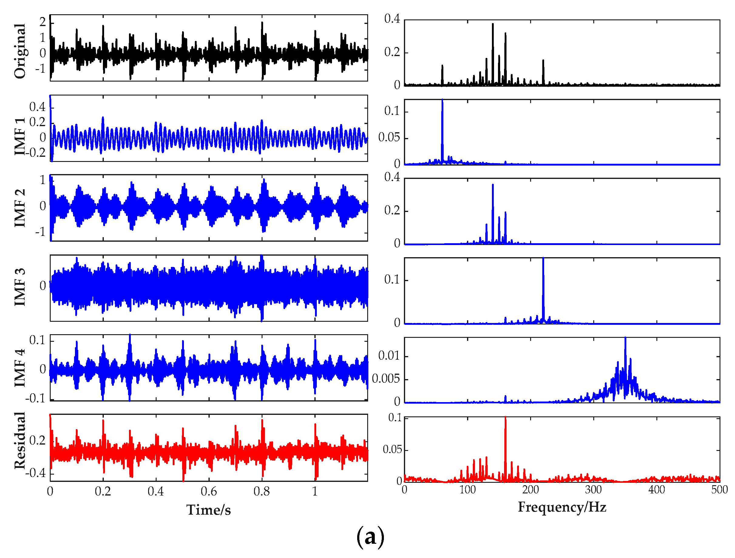
It can be seen from

Table 7. Effective modal frequency and physical correspondence of SSA-VMD.

Modal Component	Center Frequency (Hz)	Peak Frequency (Hz)	Physical Correspondence
IMF1	14.03	12.68	2fr = 12.50 Hz; the low-frequency harmonic components of stress pulse
IMF2	36.24	37.24	6fr = 37.50 Hz; intermediate-frequency harmonic components of stress pulse
IMF3	48.99	49.92	8fr = 50.00 Hz; intermediate-frequency harmonic components of stress pulse
IMF4	105.45	112.52	18fr = 112.50 Hz; the high-order harmonic of rotating frequency, located in the harmonic band near the frequency fBP = 131.25 Hz of the bucket passing through, reflects the periodic characteristics of the jet impact
IMF5	312.68	299.52	False mode, for residual noise
IMF6	429.35	437.4	The natural vibration frequency of the bucket structure is excited by the jet impact
IMF7	441.57	443.74	The natural vibration frequency of the bucket structure is close to the IMF6 frequency
IMF8	449.03	450.08	The natural vibration frequency of the bucket structure constitutes a dense high-frequency modal group with IMF6 and IMF7

that SSA-VMD outputs eight IMF components, and seven effective modes are retained after eliminating the false mode IMF5. By matching the peak frequency of each IMF with the integer multiple harmonics of the unit frequency f_r = 6.25 Hz, the deviation between the peak frequency of IMF1 ~ IMF4 and the corresponding harmonics is within 0.5 Hz. Among them, IMF1, IMF2 and IMF3 correspond to 2f_r, 6f_r and 8f_r respectively, reflecting the harmonic components of the bucket stress pulse. The peak frequency of IMF4 corresponds to 18f_r, and the center frequency is slightly lower. This may be due to the asymmetry of the spectrum distribution of this mode. Its frequency is in the harmonic band near the bucket passing frequency f_BP. Although it is not directly equal to f_BP, it still reflects the periodic stress response caused by jet impact.

The IMF6 ~ IMF8 frequencies are higher, and the three constitute a dense high-frequency modal group, which has significantly exceeded the distribution range of the rotating frequency harmonics and is more likely to correspond to the natural vibration frequency of the bucket structure, resulting in free attenuation oscillation under jet impact excitation. The above analysis shows that SSA-VMD can effectively separate the frequency components of different physical sources from the non-stationary signal of bucket runners, analyze the harmonic structure of the stress pulse in the low-frequency band, and capture the natural vibration characteristics of the bucket structure in the high-frequency band, which verifies the applicability of the method in the feature extraction of engineering signals.

3.2.4. Quantitative Comparison of Decomposition Quality (Quantitative Comparison of Decomposition Quality of the Measured Signal)

Table 8. Performance indicators. (Performance indicators of the measured signal.)

Optimistic Algorithm	Kopt	Kspurious	αopt	Sover	Sunder	ηunder	ηr	T (s)
VMD	7	2	2000	10	8	0.48%	40.00%	-
SSA-VMD	8	1	8610	9	8	0.01%	28.57%	107.8
PSO-VMD	12	5	2040	10	8	0.10%	28.57%	176.4
WOA-VMD	10	5	3800	10	8	1.07%	40.00%	220.0
GWO-VMD	13	7	4880	10	8	1.55%	33.33%	171.5

shows the quantitative comparison results of five methods on eight performance indicators.

From the perspective of the number of modes, SSA-VMD outputs K_opt = 8, and the number of false modes is the lowest. There is only one false mode, and the number of effective modes after removal is K_eff = 7. Although the number of modes of PSO-VMD and WOA-VMD is different, which is 12 and 10 respectively, the number of false modes is the same, which is five. The false mode of WOA-VMD accounts for 50%, indicating that its parameter combination also has an over-decomposition tendency. The number of modes of GWO-VMD is 13, and the number of false modes is seven.

From the perspective of the penalty factor α, VMD adopts the empirical default value of 2000. SSA-VMD selects α_opt = 8610, which is over four times the default value. The significantly elevated penalty factor provides a strong bandwidth constraint, enabling VMD to effectively separate closely spaced frequency components while producing only one false mode, which demonstrates that SSA successfully identified a high-quality parameter combination. PSO-VMD selects α_opt = 2040, nearly identical to the default value, indicating that the algorithm failed to meaningfully adjust the bandwidth constraint during the optimization process. WOA-VMD selects α_opt = 3800, representing a moderate increase, while GWO-VMD selects α_opt = 4880, a higher value; however, both algorithms still produce five and seven false modes respectively, suggesting that the penalty factor alone is insufficient without an appropriate modal number to achieve clean decomposition.

From the perspective of the degree of over-decomposition, in addition to the SSA-VMD score of nine points, there is one over-decomposition event in the effective mode; the over-decomposition scores of the other four methods were all 10 points.

From the perspective of the degree of under-decomposition, the under-decomposition scores of the five methods are all eight points, indicating that there are two under-decomposition events in the effective mode, indicating that there may be two physical components with similar frequencies in the measured signal, and the frequency interval is close to the separation limit of VMD. Current parameter optimization strategies have failed to completely separate these two components. However, from the perspective of the proportion of under-decomposition, SSA-VMD and PSO-VMD have the lowest proportion of under-decomposition, both of which are 28.57%; WOA-VMD and VMD had the highest proportion of under-decomposition, both of which were 40%, indicating that the decomposition was not complete, and the adjacent components were not effectively separated.

From the perspective of the residual energy ratio, the residual energy ratio of SSA-VMD is the lowest, which is 0.01%. The reason is that the parameter combination optimized by SSA just makes the sum of the eight modes of VMD highly approach the original signal, indicating that the modal component captures the original signal energy more completely and the decomposition fidelity is high.

From the perspective of computational efficiency, SSA-VMD achieves the shortest optimization time of T = 107.8 s, which is attributed to the strong global search capability and fast convergence of the sparrow search algorithm. GWO-VMD and PSO-VMD require 171.5 s and 176.4 s, respectively, approximately 1.6 times that of SSA-VMD, reflecting their relatively slower convergence under the multi-parameter optimization landscape. WOA-VMD consumes the longest time of T = 220 s, over twice that of SSA-VMD, which is related to its large search space exploration and slower convergence speed. Since VMD uses fixed empirical parameters without an optimization process, no computation time is recorded.

In summary, from the perspective of the number of modes, SSA-VMD produces the fewest false modes, and the parameter combination is the most accurate for the division of signal components. From the penalty factor perspective, SSA-VMD selects α_opt = 8610, the highest among all methods, which provides a strong bandwidth constraint and enables effective separation of closely spaced frequency components, whereas PSO-VMD barely adjusts this parameter from the default value. From the perspective of the degree of over-decomposition, SSA-VMD is the only method that has over-decomposition events, but its over-decomposition score is still nine points, and the degree of over-decomposition is relatively light. Although the other four methods do not have over-decomposition, they all cost a high number of modes or false modes. From the perspective of the degree of under-decomposition, there are two under-decomposition events in each of the five methods, indicating that there are indeed two physical components in the measured signal whose frequency intervals are close to the VMD separation limit. SSA-VMD and PSO-VMD have the lowest proportion of under-decomposition, and the separation effect is relatively good. From the perspective of the proportion of residual energy, SSA-VMD achieves a complete capture of the original signal energy with a very low residual energy of 0.01%, and the decomposition fidelity is the highest among the five methods. From the perspective of computational efficiency, SSA-VMD requires only 107.8 s, the shortest among all optimization algorithms, while WOA-VMD takes the longest at 220 s. Therefore, SSA-VMD has the best comprehensive performance in the decomposition of measured bucket stress signal across all eight performance indicators, which verifies the effectiveness of SSA-optimized VMD parameter combination in practical engineering signal processing.

An important finding of this study is that the fitness value does not perfectly correlate with decomposition quality. SSA-VMD consistently exhibits slightly higher fitness than PSO/GWO, yet achieves superior decomposition metrics (fewer spurious modes and higher Sunder). On the measured signal, PSO and GWO converge to identical fitness values (0.2221) with zero variance, suggesting convergence to the same local optimum that minimizes the fitness function but produces excessive over-decomposition. On the constructed signal, although PSO and GWO achieve lower fitness than SSA, their decomposition quality remains inferior. SSA’s broader exploration identifies parameter combinations with better physical meaning, even when the proxy fitness is not minimized. This finding validates the necessity of the multi-indicator evaluation system proposed in this paper, as relying solely on fitness would mislead the optimization toward suboptimal decomposition.

3.2.5. Comparison with Deterministic Search Baselines

Note that the following baseline comparison reports statistical results over 30 independent SSA-VMD runs. The mean optimal parameters (K = 8.2 ± 1.0; α = 8465 ± 492) are consistent with the single-run optimal result (K = 8; α = 8610) used in the preceding decomposition analysis, confirming the reliability of the selected parameters.

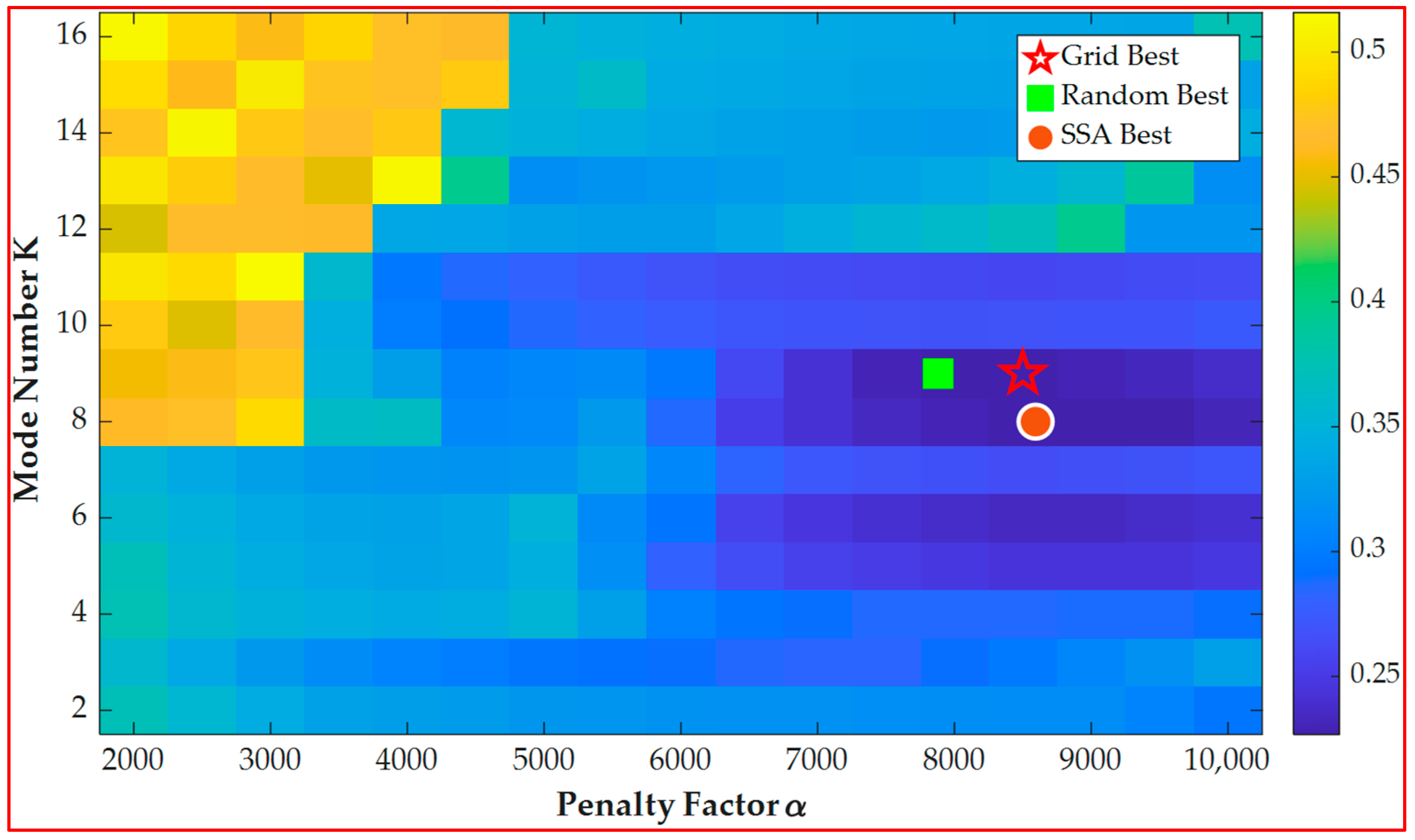
Two deterministic search baselines were implemented to validate the effectiveness of the metaheuristic optimization. Grid search exhaustively evaluated all 255 combinations of K ∈ {2, 3, …, 16} and α ∈ {2000, 2500, …, 10,000}. Random search uniformly sampled 255 random (K, α) pairs from the same ranges. Both baselines used the same fitness function as SSA-VMD.

As shown in

Table 9. Comparison of SSA-VMD with deterministic search baselines.

Method	Evals	Kopt	αopt	Fitness	Sover	Sunder	T (s)
Grid search	255	9	8500	0.2268	10	8	485.1
Random Search	255	9	7881	0.2268	10	8	447.3
SSA-VMD	500	8.2 ± 1.0	8465 ± 492	0.2269 ± 0.0058	10	9	285.9

, all three methods identify K = 8–9 as the optimal mode number, with comparable fitness values (0.2268–0.2269) and perfect over-decomposition scores (S_over = 10). SSA-VMD achieves the highest under-decomposition score (S_under = 9 vs. 8), indicating that its continuous-domain search identifies parameter combinations with more thorough component separation.

Figure 15 presents the fitness landscape from grid search, with the optimal solutions from all three methods marked. The SSA-VMD solution lies in a region adjacent to but not identical with the grid search optimum, demonstrating that metaheuristic search can explore intermediate parameter values that fixed grids cannot reach.

4. Conclusions

In this paper, aiming at the problem of modal decomposition of non-stationary stress signals of bucket runners, four optimization algorithms, SSA, PSO, WOA and GWO, were combined with VMD to construct four optimized VMD methods. By constructing two examples of signals and measured signals, the fitness curve, time–frequency decomposition effect and eight performance indicators were systematically compared and analyzed. The main conclusions are as follows:

(1) On the constructed signal, the four algorithms achieve comparable fitness values with no statistically significant difference (Wilcoxon p > 0.05). SSA-VMD demonstrates the most consistent search behavior (std = 0.0059) and outputs K_opt = 9, consistent with the true component count. Although GWO achieves the lowest mean fitness (0.1642), its decomposition quality is inferior to SSA-VMD, indicating that fitness alone is insufficient to evaluate optimization performance.

(2) On the measured stress signal of the 4# bucket runner, SSA-VMD produces the fewest spurious modes (3), the highest over-decomposition score (S_over = 10), and the highest under-decomposition score (S_under = 9), effectively separating the harmonic components and natural vibration frequencies of the bucket structure. The calculation time of SSA-VMD (123.1 s) is about 3.5 times faster than that of PSO-VMD (432.4 s).

(3) The quantitative evaluation system of decomposition quality based on eight evaluation indexes proposed in this paper comprehensively measures the decomposition quality of VMD from eight performance indexes, the optimal mode number, optimized penalty factor, false mode number, over-decomposition score, under-decomposition score, under-decomposition proportion, residual energy proportion, and computation time, which overcomes the one-sidedness of single-index evaluation and provides a systematic evaluation method for optimizing the performance evaluation of VMD parameter combination.

(4) SSA’s multi-role division mechanism enables an effective balance between exploration and exploitation, avoiding premature convergence to local optima that appear favorable in fitness but yield inferior decomposition quality. An important finding is that the fitness value does not perfectly correlate with decomposition quality: SSA-VMD consistently exhibits slightly higher fitness than PSO/GWO yet achieves superior decomposition metrics. While the fitness values are comparable across algorithms, SSA-VMD consistently achieves superior decomposition quality, providing reliable method support for accurate decomposition of non-stationary bucket runner signals.

(5) Future work will extend the robustness evaluation to broader signal conditions, validate the method on fault-seeded experiments, and investigate online VMD variants for real-time monitoring.

Several limitations should be noted. The synthetic-signal robustness experiments, while covering multiple SNR levels and noise types, do not exhaustively address all signal conditions, such as varying frequency distances and modulation strengths. The method has not yet been validated on signals containing known faults. Additionally, the optimization process requires approximately 500 VMD evaluations per run, which may limit real-time applicability.

References

1. Sun, L.; Fan, W.; Zhou, H.; Wang, Z.; Guo, P. Numerical Assessment of the Hydrodynamic Excitation Characteristics of a Pelton Turbine. Sustainability 2024, 16, 10667. [Google Scholar] [CrossRef]
2. Mettille, M.; Decaix, J.; Bullani, A.; Valluy, B.; Münch-Alligné, C. Non-viscous flow simulations of six jet Pelton turbines: The effect of jet interference and of erosion on the performance of the runner. In Proceedings of the 9th IAHR Meeting of the WorkGroup on Cavitation and Dynamic Problems in Hydraulic Machinery and Systems-IAHRWG, Universitatea Politehnica Timisoara, Timisoara, Romania, 10–12 October 2025; Volume 1483. [Google Scholar] [CrossRef]
3. Egusquiza, M.; Egusquiza, E.; Valero, C.; Presas, A.; Valentín, D.; Bossio, M. Advanced condition monitoring of Pelton turbines. Measurement 2018, 119, 46–55. [Google Scholar] [CrossRef]
4. Egusquiza, M.; Egusquiza, E.; Valentin, D.; Valero, C.; Presas, A. Failure investigation of a Pelton turbine runner. Eng. Fail. Anal. 2017, 81, 234–244. [Google Scholar] [CrossRef]
5. Xu, S.; Dao, F.; Zeng, Y.; Qian, J. Fault diagnosis of hydro-turbine runner based on improved masking signal method incorporate RLMD. Appl. Acoust. 2025, 228, 110371. [Google Scholar] [CrossRef]
6. Peng, Z.; Chu, F. Application of the wavelet transform in machine condition monitoring and fault diagnostics: A review with bibliography. Mech. Syst. Signal Process. 2004, 18, 199–221. [Google Scholar] [CrossRef]
7. Huang, N.; Shen, Z.; Long, S.; Wu, M.; Shih, H.; Zheng, Q.; Yen, N.; Tung, C.; Liu, H. The empirical mode decomposition and the Hilbert spectrum for nonlinear and non-stationary time series analysis. Proc. R. Soc. A Math. Phys. Eng. Sci. 1998, 454, 903–995. [Google Scholar] [CrossRef]
8. Xiao, W.; Gui, Z.; Lu, Z.; Xiao, R.; Tao, R. Pressure pulsation of pump turbine at runaway condition based on Hilbert Huang transform. Front. Energy Res. 2024, 12, 1344676. [Google Scholar] [CrossRef]
9. Dai, J.; Tang, J.; Huang, S.; Wang, Y. Signal-Based Intelligent Hydraulic Fault Diagnosis Methods: Review and Prospects. Chin. J. Mech. Eng. 2019, 32, 75. [Google Scholar] [CrossRef]
10. Wang, F. Pulsation Signals Analysis of Turbocharger Turbine Blades Based on Optimal EEMD and TEO. Pol. Marit. Res. 2019, 26, 78–86. [Google Scholar] [CrossRef]
11. Wang, W.; Chen, Q.; Yan, D.; Geng, D. A novel comprehensive evaluation method of the draft tube pressure pulsation of Francis turbine based on EEMD and information entropy. Mech. Syst. Signal Process. 2019, 116, 772–786. [Google Scholar] [CrossRef]
12. Dragomiretskiy, K.; Zosso, D. Variational Mode Decomposition. IEEE Trans. Signal Process. 2014, 62, 531–544. [Google Scholar] [CrossRef]
13. Xiao, Q.; Li, S.; Zhou, L.; Shi, W. Improved Variational Mode Decomposition and CNN for Intelligent Rotating Machinery Fault Diagnosis. Entropy 2022, 24, 908. [Google Scholar] [CrossRef] [PubMed]
14. Lu, Z.; Tao, R.; Xiao, R.; Li, P. Forecasting the hydropower unit vibration based on adaptive variational mode decomposition and neural network. Appl. Soft Comput. 2024, 150, 111040. [Google Scholar] [CrossRef]
15. An, X.; Yang, J. Denoising of hydropower unit vibration signal based on variational mode decomposition and approximate entropy. Trans. Inst. Meas. Control 2016, 38, 282–292. [Google Scholar] [CrossRef]
16. Wang, W.; Guo, S.; Zhao, S.; Lu, Z.; Xing, Z.; Jing, Z.; Wei, Z.; Wang, Y. Intelligent Fault Diagnosis Method Based on VMD-Hilbert Spectrum and ShuffleNet-V2: Application to the Gears in a Mine Scraper Conveyor Gearbox. Sensors 2023, 23, 4951. [Google Scholar] [CrossRef] [PubMed]
17. Jian, J.; Lu, Z.-R.; Liu, J.; Wang, L. De-mixing variational mode decomposition and its application on operational modal analysis in the presence of closely spaced modes. Measurement 2025, 242, 116057. [Google Scholar] [CrossRef]
18. Kennedy, J.; Eberhart, R. Particle swarm optimization. In Proceedings of the 1995 IEEE International Conference on Neural Networks (ICNN 95), University of Western Australia, Perth, Australia, 27 November–1 December 1995; pp. 1942–1948. [Google Scholar] [CrossRef]
19. Hu, H.; Ao, Y.; Yan, H.; Bai, Y.; Shi, N. Signal Denoising Based on Wavelet Threshold Denoising and Optimized Variational Mode Decomposition. J. Sens. 2021, 2021, 5599096. [Google Scholar] [CrossRef]
20. Mirjalili, S.; Lewis, A. The Whale Optimization Algorithm. Adv. Eng. Softw. 2016, 95, 51–67. [Google Scholar] [CrossRef]
21. Miao, Y.; Zhao, M.; Makis, V.; Lin, J. Optimal swarm decomposition with whale optimization algorithm for weak feature extraction from multicomponent modulation signal. Mech. Syst. Signal Process. 2019, 122, 673–691. [Google Scholar] [CrossRef]
22. Fang, C.; Chen, Y.; Deng, X.; Lin, X.; Han, Y.; Zheng, J. Denoising method of machine tool vibration signal based on variational mode decomposition and Whale-Tabu optimization algorithm. Sci. Rep. 2023, 13, 1505. [Google Scholar] [CrossRef] [PubMed]
23. Mirjalili, S.; Mirjalili, S.M.; Lewis, A. Grey Wolf Optimizer. Adv. Eng. Softw. 2014, 69, 46–61. [Google Scholar] [CrossRef]
24. Li, H.; Li, S.; Sun, J.; Huang, B.; Zhang, J.; Gao, M. Ultrasound signal processing based on joint GWO-VMD wavelet threshold functions. Measurement 2024, 226, 114143. [Google Scholar] [CrossRef]
25. Jin, Z.; He, D.; Wei, Z. Intelligent fault diagnosis of train axle box bearing based on parameter optimization VMD and improved DBN. Eng. Appl. Artif. Intell. 2022, 110, 104713. [Google Scholar] [CrossRef]
26. Xue, J.; Shen, B. A novel swarm intelligence optimization approach: Sparrow search algorithm. Syst. Sci. Control Eng. 2020, 8, 22–34. [Google Scholar] [CrossRef]
27. Du, H.; Wang, J.; Qian, W.; Zhang, X. An Improved Sparrow Search Algorithm for the Optimization of Variational Modal Decomposition Parameters. Appl. Sci. 2024, 14, 2174. [Google Scholar] [CrossRef]
28. Lyu, G.; Luo, C.; Wu, S.; Wang, C.; Ma, W.; Yang, M.; Wang, P.; Yang, S. An enhanced variational mode decomposition method for processing hydrodynamic data of underwater gliders. Measurement 2025, 244, 116468. [Google Scholar] [CrossRef]
29. Cheng, W.; Zhou, Q.; Wu, S.; Xing, J.; Chen, X.; Du, S.; Xu, Z.; Zhang, R. EI-ISOA-VMD: Adaptive denoising and detrending method for nuclear circulating water pump impeller. Measurement 2025, 242, 115890. [Google Scholar] [CrossRef]
30. Vashishtha, G.; Chauhan, S.; Yadav, N.; Kumar, A.; Kumar, R. Adaptive MOMEDA model based variational mode decomposition for Pelton wheel fault detection. Eng. Res. Express 2022, 4, 025044. [Google Scholar] [CrossRef]
31. Fang, M.; Zhang, F.; Yang, Y.; Tao, R.; Xiao, R.; Zhu, D. The influence of optimization algorithm on the signal prediction accuracy of VMD-LSTM for the pumped storage hydropower unit. J. Energy Storage 2024, 78, 110187. [Google Scholar] [CrossRef]
32. Fang, M.; Zhang, F.; Cao, Z.; Tao, R.; Xiao, W.; Zhu, D.; Gui, Z.; Xiao, R. Prediction accuracy improvement of pressure pulsation signals of reversible pump-turbine: A LSTM and VMD-based optimization approach. Energy Sci. Eng. 2024, 12, 102–116. [Google Scholar] [CrossRef]
Figure 1. Flow chart of adaptive selection of VMD parameters based on optimization algorithm.
Applsci 16 07817 g001
Figure 2. Fitness landscape in the K dimension at different α-values.
Applsci 16 07817 g002
Figure 3. Spearman rank correlation of fitness rankings across tolerance coefficients r (*** p < 0.001).
Applsci 16 07817 g003
Figure 4. Comparison of optimal mode number Kopt across fitness function variants.
Applsci 16 07817 g004
Figure 5. Fitness curves of different algorithms (Fitness curves of different algorithms for the structural signal): (a) SSA-VMD fitness curve. (b) PSO-VMD fitness curve. (c) WOA-VMD fitness curve. (d) GWO-VMD fitness curve.
Applsci 16 07817 g005
Figure 6. Decomposition of time–frequency diagrams by different algorithms (Decomposition of time-frequency diagrams by different algorithms for the structural signal) (all amplitude units are MPa, and black lines represent the original signal, blue lines represent the IMF components, and red lines represent the residual.): (a) VMD decomposition time–frequency diagram. (b) SSA-VMD (SSA-VMD) decomposition time–frequency diagram. (c) PSO-VMD (PSO-VMD) decomposition time–frequency diagram. (d) WOA-VMD (WOA-VMD) decomposition time–frequency diagram. (e) GWO-VMD (GWO-VMD) decomposition time–frequency diagram.
Applsci 16 07817 g006aApplsci 16 07817 g006bApplsci 16 07817 g006c
Figure 7. IMF energy distribution across different K values.
Applsci 16 07817 g007
Figure 8. Sensitivity analysis of the scaling factor s on sub-mode frequency separation for each valid IMF (In each subplot, blue circle markers represent the center frequency of sub-mode 1 and red square markers represent the center frequency of sub-mode 2 as a function of the scaling factor s.).
Applsci 16 07817 g008
Figure 9. Validation of scoring system: Sover and Sunder vs. K.
Applsci 16 07817 g009
Figure 10. Sensitivity analysis of threshold parameters: (a) λ1 on Sover (K = 14); (b) λ2 on Sunder (K = 7).
Applsci 16 07817 g010
Figure 11. Comparison of fitness distribution across SNR levels for four algorithms.
Applsci 16 07817 g011
Figure 12. The position of bucket runner and measuring point position.
Applsci 16 07817 g012
Figure 13. The fitness curves of different algorithms (Fitness curves of different algorithms for the measured signal): (a) SSA-VMD fitness curve. (b) PSO-VMD fitness curve. (c) WOA-VMD fitness curve. (d) GWO-VMD fitness curve.
Applsci 16 07817 g013
Figure 14. Decomposition of time–frequency diagram by different algorithms (Decomposition of time-frequency diagrams by different algorithms for the measured signal) (all amplitude units are MPa, and black lines represent the original signal, blue lines represent the IMF components, and red lines represent the residual.): (a) VMD decomposition time–frequency diagram. (b) SSA-VMD (SSA-VMD) decomposition time–frequency diagram. (c) PSO-VMD (PSO-VMD) decomposition time–frequency diagram. (d) WOA-VMD (WOA-VMD) decomposition time–frequency diagram. (e) GWO-VMD (GWO-VMD) decomposition time–frequency diagram.
Applsci 16 07817 g014aApplsci 16 07817 g014bApplsci 16 07817 g014c
Figure 15. Grid search fitness landscape with optimal solutions from three methods.
Applsci 16 07817 g015