A Data-Driven Framework for Condition Monitoring and Early Warning of Low-Efficiency Events in Photovoltaic Systems

Abstract

Reliable photovoltaic (PV) operation requires monitoring strategies that can detect performance degradation before it develops into persistent efficiency loss. This study proposes an interpretable data-driven framework for condition monitoring and early warning of low-efficiency events using only inverter-based electrical measurements. The novelty of this study lies in its focus on detecting low-efficiency operating conditions from inverter electrical data, rather than merely classifying individual PV fault types. Thirty-minute operational data from a 110 kW grid-connected PV plant in Kastamonu, Türkiye, covering January 2023–December 2025, were analyzed. Phase currents, phase voltages, total active power, and DC power were transformed into electrical health indicators, including mean current, mean voltage, current and voltage variability, phase imbalance index, and conversion efficiency. Correlation and imbalance analyses showed highly synchronized three-phase operation, with a mean phase imbalance index of 0.004865. Conversion efficiency remained stable, with an instantaneous mean of 0.964. Generalized Additive Model results explained 66.4% of efficiency variability and identified mean current as the dominant nonlinear determinant, while phase imbalance acted as a secondary but significant factor. A Random Forest classifier achieved 96.34% accuracy, 3.87% out-of-bag error, and 53.4% recall for rare low-efficiency events. Decision-tree rules indicated high risk when mean current fell below 9.4 A and very low risk above 12 A. The framework provides a practical, sensor-minimal, and interpretable approach for PV performance monitoring and proactive maintenance.

1. Introduction

Photovoltaic (PV) systems are playing an increasingly important role in meeting the growing energy demand with sustainable resources, and their installed capacity is rapidly increasing worldwide. Thanks to technological advancements and falling costs, large-scale solar power plants, in particular, have become a significant component of the electricity generation portfolio [1]. However, the economic success of PV systems depends not only on their installed power capacity but also on their ability to operate efficiently and reliably over the long term. Therefore, continuous monitoring of system performance and early identification of situations that may lead to efficiency losses have become an important research area in recent years [2,3].

Numerous factors may adversely affect photovoltaic energy production and reduce conversion efficiency. These include partial shading, soiling, module mismatch, hot spot formation, bypass diode failures, electrical connection problems, inverter-related abnormalities, and various degradation mechanisms Although these phenomena arise from different physical causes, they often lead to similar operational consequences, including reduced power output, lower conversion efficiency, and ultimately economic losses. Therefore, in modern photovoltaic system operation, it is important not only to identify specific fault types but also to detect operating conditions that may adversely affect system performance at an early stage, before they develop into more persistent efficiency losses [4,5,6].

From an operational perspective, the impact of a fault on system performance and energy production is more significant than its underlying physical cause. Partial shading, contamination, electrical imbalances, and equipment-related problems, although stemming from different mechanisms, generally lead to similar performance losses such as reduced power generation and decreased system efficiency. Therefore, in recent years, condition monitoring and performance-oriented monitoring approaches, which focus on the early detection of performance losses rather than simply diagnosing specific fault types, significantly contribute to maintenance and operational activities regardless of the source of the faults [7,8]. On the other hand, modern photovoltaic power plants continuously generate large amounts of operational data from inverters and SCADA systems. Electrical variables such as phase currents, phase voltages, active power, and DC power contain important information about the system’s operating characteristics [9,10]. However, existing studies have predominantly focused on power forecasting, fault detection, and fault classification, whereas comparatively less attention has been paid to the development of interpretable electrical condition indicators for the early detection of performance degradation in photovoltaic systems [5,8]. Recent advances in machine learning have considerably improved photovoltaic monitoring and fault diagnosis by employing deep learning architectures, hybrid models, image-based inspection techniques, and multi-sensor data fusion. While these approaches have achieved promising predictive performance, many rely on additional environmental sensors, thermal or visual imaging, or computationally intensive models that reduce deployment flexibility and model interpretability. Consequently, relatively few studies have addressed the development of sensor-minimal and interpretable early-warning frameworks capable of identifying emerging performance degradation using only routinely available inverter measurements. This gap highlights the need for practical monitoring approaches that combine operational simplicity, explainable decision-making, and early detection of low-efficiency operating conditions.

This study proposes a data-driven and interpretable framework for evaluating the electrical condition of photovoltaic systems and early detection of low-efficiency events using only inverter-based operational electrical measurements. For this purpose, electrical condition indicators such as average current, average voltage, current variability, voltage variability, and Phase Imbalance Index were derived from three-phase current and voltage measurements. In the first stage, the electrical stability and phase balance of the system were examined using correlation analyses and imbalance indicators. Subsequently, the photovoltaic conversion efficiency was analyzed at different time scales to evaluate the temporal dynamics of system performance. Generalized Additive Models (GAMs) were used to reveal nonlinear relationships between efficiency and electrical condition indicators, while Random Forest (RF) and Decision Tree (DT) methods were employed to identify low-efficiency events and develop early warning rules. The workflow is summarized in Figure 1.

Although inverter-based monitoring and SCADA data have been widely used in photovoltaic research, most existing studies employ these data either for fault diagnosis or for improving predictive accuracy through increasingly sophisticated machine learning models. The present study adopts a different perspective. Rather than identifying specific fault categories, the proposed framework evaluates the electrical operating condition of the PV system and detects situations that may precede sustained efficiency loss. The methodological contribution lies in integrating electrical health assessment, phase imbalance analysis, nonlinear efficiency modelling, probabilistic risk estimation, and interpretable decision rules into a single operational workflow using only routinely available inverter measurements. As a result, the framework provides information that is directly applicable to condition monitoring and maintenance decision-making without requiring additional sensing infrastructure.

Accordingly, the main contributions of this study can be summarized as follows:

• An operational monitoring framework is developed that uses only routinely available inverter measurements to identify emerging low-efficiency operating conditions.
• Electrical health indicators describing current behavior, voltage behavior, and phase imbalance are derived and linked to photovoltaic conversion efficiency.
• Generalized Additive Models and Random Forest are employed in a complementary manner to explain efficiency degradation while simultaneously estimating the probability of low-efficiency events.
• The analytical findings are translated into practical decision rules that can support routine condition monitoring and maintenance planning.

2. Literature Review

Given the wide variety of factors that can negatively impact photovoltaic system performance, there is a growing need for monitoring frameworks capable of detecting performance degradation at an early stage [11]. Current studies utilize various techniques such as infrared thermography, electroluminescence imaging, current-voltage (I-V) curve analysis, additional sensor-based measurement systems, and artificial intelligence methods [12,13,14]. In recent years, machine learning and deep learning methods have become widely used in fault detection and performance evaluation of photovoltaic systems [15,16,17].

Abdelsattar et al. [17] have comprehensively evaluated advanced Machine Learning (ML) models such as CatBoost, Gradient Boosting (GB), Random Forest, and XGBoost for fault detection and performance anomaly identification in PV systems. In their tests using a large dataset of approximately 97,333 observations, they stated that all evaluated models showed high success rates, but the CatBoost model exhibited the highest performance in fault detection. Zong et al. proposed a time-series and SVM-based model to distinguish between shading and aging faults exhibiting similar electrical characteristics in PV arrays. They reported that the method, tested with an LED simulation device, achieved a diagnostic accuracy of 99.5% for known fault characteristics and 95.2% for unknown characteristics. The results demonstrate that this approach offers a proactive and reliable solution for improving the operational safety and efficiency of PV systems [18]. Amiri et al. proposed a hybrid deep learning approach combining Convolutional Neural Network (CNN) and Bi-Gated Recurrent Unit (Bi-GRU) architectures for fault detection and diagnosis in PV systems. In the study, a database representing healthy and faulty operating conditions was created, and different fault types such as open circuit, short circuit, and partial shading were detected and classified [19]. Ling et al. proposed a deep learning-based approach for detecting faults in PV panels using infrared imagery. Combining CNN-based edge detection with the You Only Look Once version 5 (YOLOv5) classifier, the method yielded successful results on data from real PV power plants [20]. Veerasamy et al. proposed a Discrete Wavelet Transform (DWT) and Long Short-Term Memory (LSTM) based approach for detecting High Impedance Faults (HIFs) in PV integrated power systems. In their study, which utilized features obtained from three-phase current signals, the proposed LSTM model reported a classification accuracy of 91.21% and a success rate of 92.42% in detecting high impedance faults [21]. Alrifaey et al. developed a hybrid deep learning model consisting of Wavelet Packet Transform (WPT), Stacked Autoencoder (SAE), Deep Equilibrium Optimizer Algorithm (DEOA), and LSTM structures for fault detection and classification in grid-connected PV systems. The proposed method improved fault diagnosis performance through automatic feature extraction and selection, achieving an accuracy rate of 99.93% in tests [16]. Teta et al. [22] proposed a method combining transfer learning and ensemble learning for fault diagnosis in grid-connected PV systems. In the study, time series data were converted into two-dimensional images, and features extracted with MobileNet were evaluated in an ensemble classifier based on Support Vector Machines (SVM), Random Forest (RF), and Decision Tree (DT). The proposed method provided an effective approach for fault diagnosis in PV systems by achieving high accuracy in both noise-free and noisy datasets. Lodhi et al. proposed a deep learning-based stacked ensemble (DSEL) approach combining DNN (Deep Neural Network), LSTM, and Bi-LSTM (Bidirectional Long Short-Term Memory) models for fault detection and classification in PV arrays. The study evaluated open circuit, short circuit, bridge fault, partial shadowing, and decay faults, demonstrating that the proposed model yielded more successful results with high accuracy rates compared to existing machine learning and deep learning-based methods, both in noise-free and noisy datasets [23]. Bougoffa et al. developed a hybrid deep learning approach combining Stacked Sparse Autoencoder (SSAE) and Optimized Multi-Layer Perceptron (OMLP) for fault diagnosis in PV systems. Using current, voltage, irradiation, and module temperature data, the study demonstrated high accuracy in detecting various fault types such as open circuits, short circuits, partial shading, and module degradation [24]. Kull et al. proposed a hybrid approach combining Adaptive Deep Belief Networks (A-DBN) and Light Gradient Boosting Machine (LightGBM) for fault diagnosis in photovoltaic systems using SCADA-based real-world field data. The study classified different fault types, including open circuit, grounding, partial shading, busbar, fouling, and hot spots, using data such as DC voltage, DC current, irradiation, inverter power, module temperature, and performance ratio. The results showed that the proposed method provides an effective solution for real-time fault diagnosis in PV systems, achieving over 98% accuracy [25].

Although methods proposed in the literature have yielded successful results in fault detection and classification in photovoltaic systems, the majority of studies focus on identifying specific fault types. Furthermore, many approaches require image processing techniques, additional sensors, or complex deep learning architectures, creating various limitations in terms of interpretability and applicability in field applications. However, the number of studies that assess the overall operating status of the system using explainable indicators derived from electrical operating data and aim to identify conditions that may lead to efficiency loss at an early stage is still limited. This study proposes an interpretable condition monitoring approach based solely on electrical operating data obtained from inverter-based monitoring systems for the early detection of low-efficiency events in photovoltaic systems. The relationships between condition indicators derived from current and voltage variables and photovoltaic conversion efficiency were analyzed using GAM and RF methods. The findings were then converted into decision rules easily interpreted by operators using a DT model. Thus, the study provides a clear and practical framework focusing on the early identification of operating conditions that negatively impact system performance, rather than the classification of specific failure types. The key methodological differences between the proposed framework and representative studies reported in the literature are summarized in

Table 1. Key methodological differences between previous studies and the proposed framework.

Representative Approaches in the Literature	Proposed Framework
Fault diagnosis	Performance-oriented monitoring
Fault classification	Low-efficiency event detection
Additional sensors often required	Only inverter measurements
Separate analytical steps	Integrated workflow
Model output	Operational decision rules

.

As shown in Table 1, the proposed framework is intended to support performance-oriented condition monitoring by integrating interpretable analytical steps into a unified workflow using only routinely available inverter measurements.

3. Materials and Methods

The risk detection stage was developed to estimate the probability that the PV system would enter a low-efficiency operating regime based on electrical health indicators, phase imbalance characteristics, and efficiency-related temporal features. In PV systems, fault detection and diagnostic frameworks commonly rely on monitored electrical variables because abnormal current, voltage, and power patterns may indicate degradation, mismatch, imbalance, or incipient failure conditions [2,26]. Therefore, the proposed risk detection module formulates the problem as a supervised probabilistic classification task rather than a simple rule-based alarm mechanism. This formulation is consistent with recent PV fault diagnosis studies in which machine learning and ensemble learning approaches are used to detect nonlinear and multivariate degradation patterns [26,27].

Let t denote the monitoring time window after temporal aggregation of the original high-frequency measurements. For each window, the three-phase current and voltage measurements were defined as $I_{A,t}, I_{B,t}, I_{C,t}$ and $V_{A,t}, V_{B,t}, V_{C,t}$ respectively. The mean current and current standard deviation were calculated as:

$${\overline{I}}_t={\displaystyle \frac{I_{A,t}+I_{B,t}+I_{C,t}}{3}}$$

(1)

$$s_{I,t}=\sqrt{{\displaystyle \frac{{\left(I_{A,t}-{\overline{I}}_t\right)}^2+{\left(I_{B,t}-{\overline{I}}_t\right)}^2+{\left(I_{C,t}-{\overline{I}}_t\right)}^2}{2}}}$$

(2)

Similarly, the mean voltage and voltage standard deviation were calculated as:

$${\overline{V}}_t={\displaystyle \frac{V_{A,t}+V_{B,t}+V_{C,t}}{3}}$$

(3)

$$s_{V,t}=\sqrt{{\displaystyle \frac{{\left(V_{A,t}-{\overline{V}}_t\right)}^2+{\left(V_{B,t}-{\overline{V}}_t\right)}^2+{\left(V_{C,t}-{\overline{V}}_t\right)}^2}{2}}}$$

(4)

The phase imbalance index was included as a key explanatory feature because electrical imbalance may reflect unequal phase loading, component mismatch, or abnormal operating conditions in three-phase PV-connected systems. The phase imbalance index was computed as:

$${\mathrm{PII}}_t={\displaystyle \frac{\mathrm{m}\mathrm{a}\mathrm{x}\left(I_{A,t},I_{B,t},I_{C,t}\right)-\mathrm{m}\mathrm{i}\mathrm{n}\left(I_{A,t},I_{B,t},I_{C,t}\right)}{{\overline{I}}_t}}$$

(5)

The conversion efficiency of the PV system was expressed as the ratio between total active AC power and total DC power:

$${\eta }_t={\displaystyle \frac{P_{\mathrm{AC},t}}{P_{\mathrm{DC},t}}}$$

(6)

where $P_{AC,t}$ is the total active power and $P_{DC,t}$ is the total DC input power. The response variable was defined as a binary low-efficiency risk indicator. For a prediction horizon h, the target variable was formulated as:

$$Y_{t,h}=\left\{\begin{array}{ll}1,& m_{t,h}<{\tau }_{\eta },\\ 0,& m_{t,h}\ge {\tau }_{\eta }.\end{array}\right.$$

(7)

where $Y_{t,h}=1$ indicates that a low-efficiency condition occurs within the future horizon h, and ${\tau }_n$ denotes the low-efficiency threshold. In this study, the low-efficiency threshold, ${\tau }_n$, was defined as the 5th percentile of the inverter conversion efficiency distribution calculated exclusively from the training dataset. Observations with efficiency values equal to or below this threshold were labelled as low-efficiency conditions. The threshold was then applied unchanged to the independent test datasets, thereby preserving the chronological independence of the evaluation periods and preventing information leakage. The percentile-based definition was preferred because no universally applicable absolute efficiency limit was available for the investigated inverter and operating conditions. Furthermore, the lower 5th percentile represents the extreme lower tail of the empirical efficiency distribution, enabling statistically rare yet operationally meaningful low-efficiency events to be identified while retaining a sufficient number of positive samples for robust model training.

The predictor vector used for risk estimation was defined as:

$$x_t=\left[{\overline{I}}_t,s_{I,t},{\overline{V}}_t,s_{V,t},{\mathrm{PII}}_t,P_{\mathrm{AC},t},{\eta }_{t-l},\Delta {\eta }_{t-l},{\mathrm{DoY}}_t,{\mathrm{ToD}}_t\right]$$

(8)

where η_t−l represents lagged efficiency, Δη_t−l represents the recent change in lagged efficiency, DoY_t denotes day-of-year, and ToD_t denotes time-of-day. Lagged and rolling-window predictors were preferred because PV monitoring data are temporally dependent and because early-warning models should rely on information available before the occurrence of the low-efficiency event.

The dataset was partitioned chronologically into a training set (70%) and an independent test set (30%). The earliest observations were assigned to the training subset for model development, while the most recent observations were reserved for performance evaluation. This chronological partitioning strategy preserves the temporal order of the photovoltaic monitoring data and prevents information leakage that could arise from random data shuffling.

Since low-efficiency events may occur less frequently than normal operating periods, class imbalance was handled through inverse-frequency class weighting:

$$w_c={\displaystyle \frac{N}{2N_c}}, c\in \{0,1\}$$

(9)

where N is the total number of training observations and N_c is the number of observations in class c. Both the Generalized Additive Model and the Random Forest model were trained to estimate the conditional risk probability:

$${\widehat{p}}_{t,h}=P\left(Y_{t,h}=1\mid x_t\right)$$

(10)

The final binary decision was obtained using a probability threshold:

$${\widehat{Y}}_{t,h}=\left\{\begin{array}{ll}1,& {\widehat{p}}_{t,h}\ge {\tau }_p,\\ 0,& {\widehat{p}}_{t,h}<{\tau }_p.\end{array}\right.$$

(11)

where ${\tau }_p$ is the operational decision threshold. When the cost of missing a low-efficiency event is higher than the cost of a false alarm, the threshold may be selected using a cost-sensitive formulation:

$${\tau }_p={\displaystyle \frac{C_{\mathrm{FP}}}{C_{\mathrm{FP}}+C_{\mathrm{FN}}}}$$

(12)

where C_FP and C_FN represent the costs of false positive and false negative decisions, respectively. Model performance was evaluated using sensitivity, specificity, precision, recall, F1-score, receiver operating characteristic analysis, precision–recall analysis, and the Brier score. ROC analysis was used to assess overall discrimination ability [28], while precision–recall analysis was emphasized under class imbalance because it is more informative when the positive class is relatively rare [29]. The Brier score was used to evaluate the accuracy of probabilistic predictions [30].

$$\mathrm{BS}={\displaystyle \frac{1}{N}}{\displaystyle \sum _{i=1}^N}{\left({\widehat{p}}_i-Y_i\right)}^2$$

(13)

3.1. Generalized Additive Model (GAM) for Interpretable Risk Estimation

A Generalized Additive Model (GAM) was employed as an interpretable statistical model to estimate the probability of low-efficiency risk [31]. GAMs extend generalized linear models by replacing strictly linear predictor effects with smooth nonlinear functions, thereby allowing the relationship between electrical indicators and risk probability to be learned from the data while retaining interpretability. This property is particularly suitable for PV risk monitoring because variables such as current level, voltage variability, phase imbalance, and active power may exhibit nonlinear associations with system degradation or low-efficiency operation.

The low-efficiency response variable was assumed to follow a Bernoulli distribution. The proposed GAM structure was formulated as:

$$\mathrm{logit}\left(p_{t,h}\right)=\mathrm{l}\mathrm{o}\mathrm{g}\left({\displaystyle \frac{p_{t,h}}{1-p_{t,h}}}\right)$$

(14)

$$\begin{gathered} \mathrm{logit}\left(p_{t,h}\right)={\beta }_0+f_1\left({\overline{I}}_t\right)+f_2\left(s_{I,t}\right)+f_3\left({\mathrm{PII}}_t\right)+f_4\left({\overline{V}}_t\right)+f_5\left(s_{V,t}\right) \\ +f_6\left(P_{\mathrm{AC},t}\right)+f_7\left({\eta }_{t-l}\right)+f_8\left(\Delta {\eta }_{t-l}\right)+f_9\left({\mathrm{DoY}}_t\right)+f_{10}\left({\mathrm{ToD}}_t\right)+f_{11}\left({\overline{I}}_t,{\mathrm{PII}}_t\right) \end{gathered}$$

(15)

where ${\beta }_0$ is the intercept, f_j(⋅) are univariate smooth functions, and $f_{11}(\overline{I_t}, {PII}_t)$ represents a two-dimensional interaction smooth between mean current and phase imbalance. The inclusion of this interaction is physically meaningful because the same imbalance level may have different operational implications under low-current and high-current regimes.

Each smooth function was represented using a penalized spline basis: Each smooth function was represented using a penalized regression spline basis. For the j-th predictor, the smooth function was expressed as:

$$f_j\left(z\right)={\displaystyle \sum _{k=1}^{K_j}}{\theta }_{jk}{b}_{jk}\left(z\right)$$

(16)

where b_jk(z) is the k-th basis function, θ_jk is the corresponding coefficient, and K_j is the basis dimension. Thin-plate regression splines were used for continuous electrical predictors because they provide a flexible and efficient basis representation for smooth nonlinear effects [32]. Cyclic smooth terms were used for temporal variables such as day-of-year and time-of-day in order to capture periodic seasonal and diurnal operating patterns.

The penalized log-likelihood function of the GAM was formulated as:

$$l_p\left(\theta \right)={\displaystyle \sum _{t=1}^N}{w}_t\left[Y_{t,h}\mathrm{l}\mathrm{o}\mathrm{g}\left(p_{t,h}\right)+\left(1-Y_{t,h}\right)\mathrm{l}\mathrm{o}\mathrm{g}\left(1-p_{t,h}\right)\right]-{\displaystyle \frac{1}{2}}{\displaystyle \sum _{j=1}^J}{\lambda }_j{\theta }_j^T{S}_j{\theta }_j$$

(17)

where w_t is the class weight, λ_j is the smoothing parameter, and S_j is the penalty matrix controlling excessive curvature in the estimated smooth functions. The smoothing parameters were estimated using restricted maximum likelihood because REML-based smoothing parameter estimation provides stable inference for semiparametric generalized models [32].

The Generalized Additive Model was implemented in R 3.0.3 using the mgcv package. Smooth terms were estimated using penalized regression splines with smoothing parameters selected by Restricted Maximum Likelihood (REML). Unless otherwise specified, the default basis dimension and optimization settings of the package were retained to avoid unnecessary model complexity while preserving interpretability.

The interpretability of the GAM was assessed through smooth partial effects. For a predictor z, the change in the odds of entering a low-efficiency regime between two operating points z_a and z_b was expressed as:

$$\mathrm{OR}\left(z_a,z_b\right)=\mathrm{e}\mathrm{x}\mathrm{p}\left[f_j\left(z_a\right)-f_j\left(z_b\right)\right]$$

(18)

An odds ratio greater than one indicates that the risk of a low-efficiency event increases when the predictor moves from z_b to z_a, holding the remaining predictors constant. In this study, this interpretation enables the identification of critical operating regions in which increasing phase imbalance, current variability, or voltage instability is associated with a higher probability of efficiency degradation. Therefore, the GAM was used not only as a predictive model but also as an explanatory layer for understanding how electrical health indicators contribute to risk formation.

Model adequacy was examined through residual diagnostics, effective degrees of freedom, smooth-term significance, validation-set performance, and concurvity checks. Smooth terms with excessive complexity but weak validation contribution were simplified to reduce overfitting. This procedure ensured that the GAM retained sufficient flexibility to capture nonlinear effects while maintaining interpretability, which is a key requirement for operation-oriented PV monitoring and decision support.

3.2. Random Forest Model for Nonlinear Risk Classification

A Random Forest classifier [33] was employed to identify operating conditions associated with low-efficiency events and to quantify the relative importance of electrical health indicators. Unlike conventional statistical models, Random Forest can capture nonlinear relationships and interaction effects without requiring predefined functional forms, making it particularly suitable for complex photovoltaic operating behavior.

Within the proposed framework, the Random Forest model served two complementary purposes. First, it was used as a predictive classifier to estimate the probability of low-efficiency operation. Second, it provided a diagnostic layer for identifying the electrical variables most strongly associated with increased efficiency-loss risk. Consequently, the model was used not only for classification but also as an operational risk-ranking tool supporting preventive maintenance decisions.

To preserve the temporal structure of the photovoltaic monitoring data, the observations were partitioned chronologically into a training set (70%) and a testing set (30%). The Random Forest classifier was trained using the training subset, while its predictive performance was evaluated on the independent chronologically held-out test subset. Chronological partitioning was preferred because adjacent photovoltaic observations are temporally dependent and random partitioning may produce overly optimistic performance estimates.

The Random Forest model was implemented using R package randomForest. The model consisted of 500 trees (ntree = 500) and the number of variables randomly sampled at each split (mtry) was defined as a default value for classification problems. All other model parameters were set to default values in the package. The variable importance was computed via permutation-based Mean Decrease Accuracy and Mean Decrease Gini.

Model interpretability was incorporated through permutation-based variable importance and partial dependence analysis. Variable importance was used to quantify the relative contribution of each predictor to low-efficiency risk estimation, while partial dependence plots were employed to examine the marginal effects of key electrical indicators on predicted risk probabilities.

The Random Forest model was interpreted jointly with the Generalized Additive Model (GAM). While GAM was used to reveal smooth and statistically interpretable relationships between electrical indicators and photovoltaic conversion efficiency, Random Forest was employed to identify nonlinear interactions, threshold-dependent behavior, and complex predictive patterns. Consistent findings across both approaches were considered stronger evidence of emerging low-efficiency operating conditions. This complementary framework combines the interpretability of GAM with the predictive flexibility of machine-learning methods, thereby enhancing the robustness of the proposed early-warning system for photovoltaic performance monitoring.

4. Experiment and Results

This section presents the methods of data collection for the implementation of the proposed methodology and the findings obtained as a result of the methodology.

4.1. Data Collection

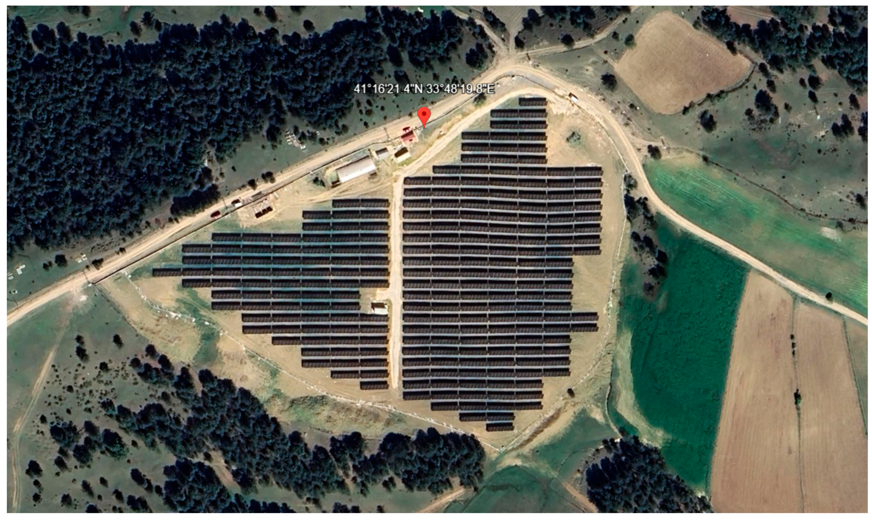
The dataset used in this study was gathered from a grid-coupled PV power facility (Figure 2) with a 110 kW installed capacity, in Kastamonu, Türkiye (Latitude: 41.2726° N, Longitude: 33.8055° E). The power plant uses monocrystalline photovoltaic panels, each with a power output of 400 Wp. The electrical characteristics of the panels used are given in

Table 2. PV panel electrical characteristics.

Label Values	Unit
Peak Power (Pmax)	400 Wp
Module Efficiency (%)	20.06
Maximum Power Voltage (Vmp)	41.10 V
Maximum Power Current (Imp)	9.75 A
Open Circuit Voltage (Voc)	49.83 V
Short Circuit Current (Isc)	10.38 A
Power Tolerance	0~+5 W
Operating Temperature	−40~+85 °C

. In practice, the operational records were obtained straight from the plant monitoring system between January 2023 and December 2025, and they were logged with a 30 min sampling interval, so everything lines up in half hour steps.

Overall, the dataset is made up only of electrical readouts that are typically already available in inverter centered monitoring systems. The stored variables cover three phase currents (Phase A, Phase B and Phase C currents), as well as three phase voltages (Phase A, Phase B and Phase C voltages), plus total DC power, total active AC power, and the cumulative daily energy yield. Together, these values help describe the electrical behavior and the conversion efficiency, or power transformation performance, of the PV installation.

Before any analysis started, the time references were synchronized and the acquired data went through standard preprocessing steps, which included data cleansing and basic consistency checks. Because the proposed method is meant to stay practical, and also be simple to deploy, we relied solely on those electrical operational measurements, with no extra environmental sensors, no thermal imaging setups, and no specialized diagnostic tools or similar instrumentation.

4.2. Analytical Structure of the Results

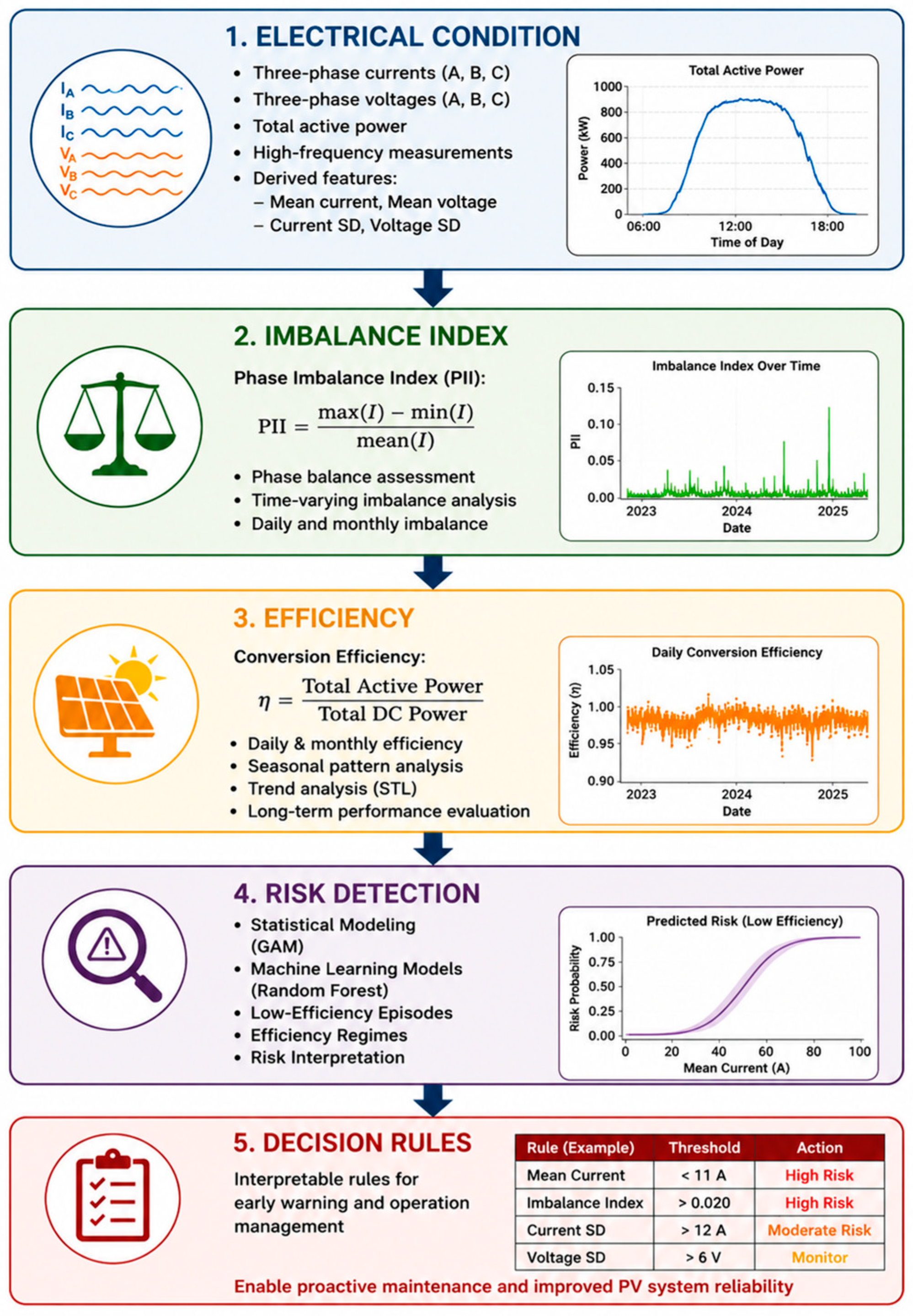
This section presents the empirical results obtained from high-resolution electrical measurements collected from a three-phase photovoltaic system. The dataset consists of 30 min operational records, including phase currents, phase voltages, total active power, and total DC power. In addition to these directly measured variables, several derived indicators were constructed to characterize the electrical behavior and conversion performance of the system. These indicators include mean current, mean voltage, current standard deviation, voltage standard deviation, the Phase Imbalance Index, and photovoltaic conversion efficiency.

The empirical analysis was designed to move from electrical health assessment to efficiency modelling and finally to early-warning risk detection. This layered structure was adopted because photovoltaic performance cannot be adequately evaluated by conversion efficiency alone. A system may exhibit high average efficiency while still experiencing transient phase imbalances, short-term loading irregularities, or low-efficiency events under specific operating conditions. Therefore, the results are organized to first examine whether the electrical system operates in a balanced and stable manner, then to identify the main determinants of conversion efficiency, and finally to assess whether low-efficiency events can be detected using interpretable machine learning models.

The first part of the analysis evaluates the electrical health of the system by examining the relationships among the three phase currents and voltages. Phase correlations, rolling correlations, and the Phase Imbalance Index are used to determine whether the three-phase structure remains synchronized over time. Daily and monthly imbalance indicators are then examined to assess whether phase imbalance exhibits temporal clustering, seasonal behavior, or signs of gradual deterioration. This step is important because phase imbalance may not always be visible from average power output alone, yet it can provide early information about operational instability.

The second part of the results focuses on photovoltaic conversion efficiency. Conversion efficiency is treated as the central performance indicator of the study because it directly reflects the relationship between DC input power and AC output power. The analysis considers instantaneous, daily, and monthly efficiency values in order to distinguish short-term fluctuations from persistent performance patterns. In addition, seasonal-trend decomposition is used to examine whether efficiency follows recurring annual patterns or shows evidence of long-term decline. This enables the study to separate normal seasonal variation from potential degradation-related behavior.

The third part of the analysis investigates the electrical determinants of efficiency. The central empirical relationship is formulated as Equation (6). This formulation allows conversion efficiency to be interpreted as a function of electrical loading, voltage behavior, phase balance, and short-term variability. Since these relationships may be nonlinear, the analysis uses a GAM to estimate smooth effects of the selected electrical indicators on efficiency. This approach makes it possible to identify whether current, voltage, or phase imbalance affects efficiency in a linear manner or whether their effects vary across operating regimes.

The final part of the results develops an early-warning framework for low-efficiency events. Random Forest classification is used to evaluate whether low-efficiency observations can be detected from high-frequency electrical variables. This model is complemented by efficiency episode analysis, efficiency regime comparison, and decision-tree-based operational threshold rules. The aim is not only to classify low-efficiency events, but also to translate model outputs into interpretable operating conditions that can support maintenance-oriented decision-making.

The Results section is organized according to three research questions. First, RQ1 asks whether high-frequency inverter-based electrical measurements indicate balanced and stable three-phase operation over time. This question is addressed by examining phase correlations, rolling correlations, the Phase Imbalance Index, and daily/monthly imbalance patterns. Second, RQ2 asks which electrical indicators explain variations in photovoltaic conversion efficiency and whether these relationships are nonlinear. This question is examined using instantaneous, daily, and monthly efficiency statistics, seasonal-trend decomposition, trend testing, and Generalized Additive Model estimation. Third, RQ3 asks whether low-efficiency operating events can be detected from high-frequency electrical measurements and whether the resulting model outputs can be converted into interpretable operational warning rules. This question is addressed using Random Forest classification, efficiency episode and regime analyses, decision tree thresholds, and operational risk rules.

Unlike conventional photovoltaic monitoring approaches that rely primarily on meteorological variables such as irradiance and temperature, the present framework uses only electrical measurements obtained directly from the inverter. This allows the development of a practical monitoring strategy that does not require additional environmental sensors. The main contribution of the results is therefore twofold: first, they show how current, voltage, and phase imbalance indicators can be used to characterize photovoltaic system health; second, they demonstrate how the same variables can be transformed into an interpretable early-warning framework for detecting low-efficiency operating conditions.

4.3. Main Empirical Findings

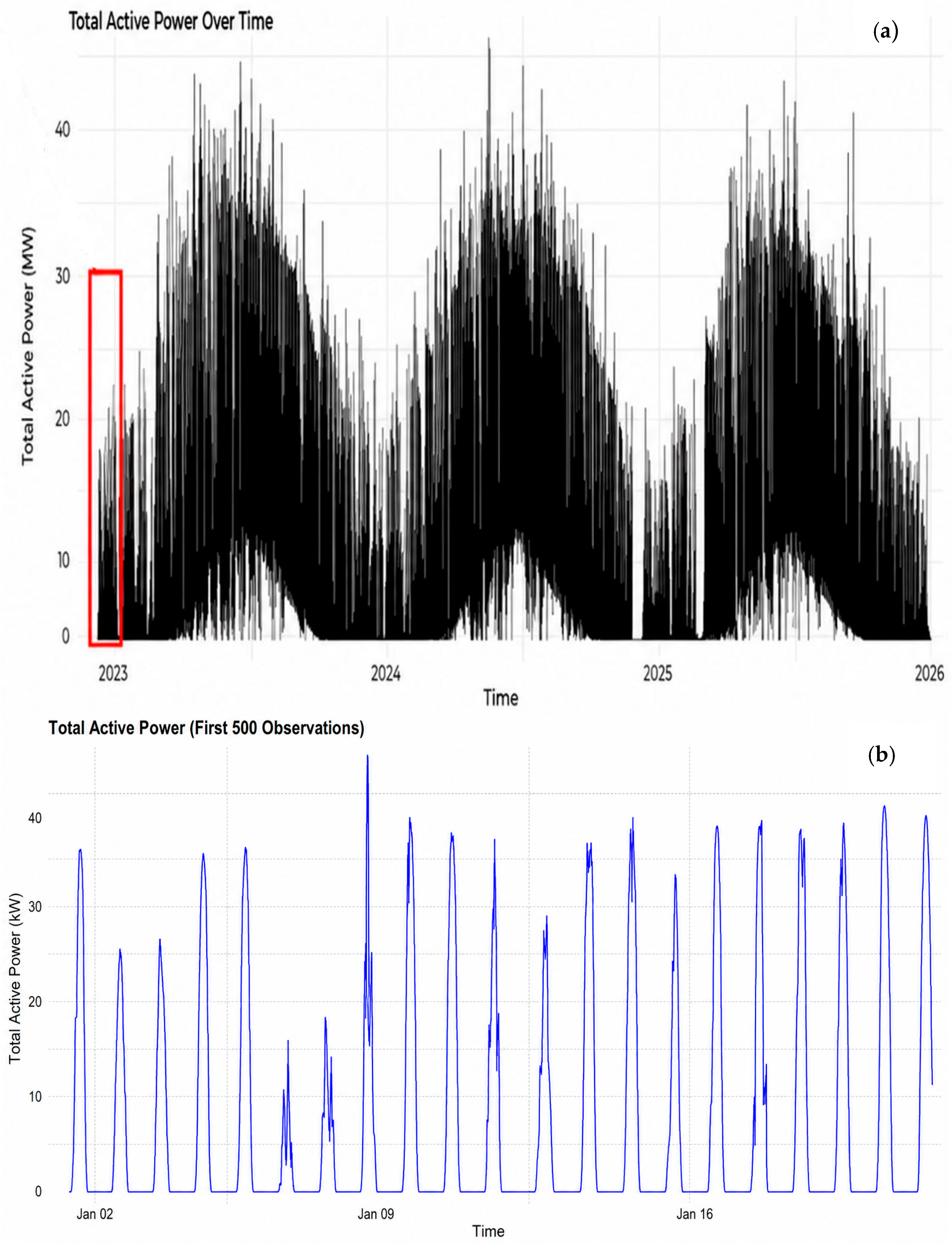
As an initial step in the empirical analysis, the temporal behavior of total active power was examined to characterize the photovoltaic generation profile, identify dominant seasonal structures, and define an analytically meaningful dataset restricted to active production periods. As shown in Figure 3a, the full-period total active power series exhibits a clear multi-scale seasonal structure. The long-term pattern indicates annual variability in power generation, while the repeated high-frequency fluctuations reflect the intraday solar production cycle. This dual-seasonal behavior suggests that photovoltaic power output is not governed only by short-term daylight availability, but is also shaped by seasonal changes in atmospheric and meteorological conditions, including solar elevation, day length, irradiance availability, and environmental operating conditions.

The magnified segment in Figure 3a and the detailed view in Figure 3b further clarify the intraday structure of the series. Power generation increases after sunrise, reaches higher levels during daylight hours, and declines toward sunset, producing a recurrent daily rise-and-fall pattern. This behavior confirms that the total active power series should not be treated as a strictly stationary process. Instead, the observed power dynamics are characterized by recurring temporal dependencies operating at different frequencies. Therefore, subsequent modelling and risk-detection analyses were designed to account for both short-term operational variability and longer-term seasonal behavior.

This visual inspection also provides the empirical justification for the data preprocessing strategy adopted in the study. Since nighttime observations correspond to structurally non-generating periods, their inclusion could distort the estimated relationships among phase currents, phase voltages, active power, DC power, conversion efficiency, and low-efficiency risk. Accordingly, observations recorded outside active production hours were excluded, and the analytical dataset was restricted to measurements collected between 07:00 and 18:30. After this filtering step, the final dataset contained approximately 27,000 high-frequency observations covering the period from 1 January 2023 to 31 December 2025. The retained observations therefore represent active photovoltaic operating conditions and provide a suitable basis for evaluating electrical health, conversion efficiency dynamics, and early-warning risk detection using inverter-based electrical measurements.

In a three-phase photovoltaic inverter system, total active power is determined by the combined contribution of phase currents, phase voltages, and the operating power factor. In its general phase-wise form, active power can be expressed as:

$$\mathrm{P} = V_A{I}_A\cos {\varphi }_A+V_B{I}_B\cos {\varphi }_B+V_C{I}_C\cos {\varphi }_C$$

(19)

where P denotes total active power, V is the line-to-line voltage, I is the line current, and $cos \varphi$ represents the power factor. Under stable inverter operation, voltage is generally maintained within a relatively narrow operating range, whereas current responds more directly to variations in solar generation and loading conditions. Therefore, total active power is expected to exhibit a stronger association with phase currents than with phase voltages.

Table 3. Correlation matrix of phase currents, phase voltages, and total active power during active PV generation periods.

Variable	Current a	Current b	Current c	Voltage a	Voltage b	Voltage c	Total Active Power
Current a	1.000	1.000	1.000	0.301	0.303	0.303	1.000
Current b	1.000	1.000	1.000	0.301	0.303	0.303	1.000
Current c	1.000	1.000	1.000	0.302	0.304	0.303	1.000
Voltage a	0.301	0.301	0.302	1.000	0.993	0.993	0.299
Voltage b	0.303	0.303	0.304	0.993	1.000	1.000	0.302
Voltage c	0.303	0.303	0.303	0.993	1.000	1.000	0.301
Total active power	1.000	1.000	1.000	0.299	0.302	0.301	1.000

reports the correlation structure among the three phase currents, three phase voltages, and total active power. It should be noted that the Pearson correlation coefficients reported in Table 3 represent global linear associations calculated over the entire observation period. Phase currents and active power exhibit pronounced diurnal patterns associated with the daily PV generation cycle, while phase voltages may display weaker concurrent temporal variations due to inverter–grid interactions. Consequently, part of the observed correlations may reflect synchronized temporal operating patterns rather than direct electrical dependence among the variables. Moreover, repeated nighttime and near-zero generation observations may inflate the apparent correlations among current- and power-related variables. Accordingly, the coefficients in Table 3 should be interpreted as descriptive indicators of system-wide co-movement and phase synchronization under a shared temporal operating cycle, rather than as evidence of direct or causal dependence. The subsequent GAM and Random Forest analyses complement this descriptive assessment by examining nonlinear relationships and threshold-dependent behavior; however, these analyses are not intended to establish causality.

To further assess the potential influence of multicollinearity, Variance Inflation Factors (VIFs) were calculated for all electrical predictors. The resulting values were 3.801 for mean current, 1.004 for mean voltage, 2.373 for the phase imbalance index, 3.641 for current standard deviation, and 1.010 for voltage standard deviation. Since all VIF values remained below the commonly accepted threshold of 5, the results indicate that multicollinearity was not sufficiently severe to compromise model interpretation. Although some predictors exhibited strong pairwise correlations, the observed level of redundancy was considered acceptable, and the full predictor set was therefore retained for the subsequent GAM and Random Forest analyses.

The results reveal an almost perfect positive correlation among the phase currents, with coefficients equal or very close to 1.00. This indicates that the current profiles of phases A, B, and C evolved in a highly synchronized manner during active generation periods. Such behavior provides initial evidence of balanced current distribution across the three phases and suggests that no substantial persistent divergence occurred among the phase current signals.

A similarly strong association was observed among the phase voltages. The voltage–voltage correlations ranged from 0.993 to 1.000, indicating a highly stable and synchronized voltage structure across the three phases. This result is consistent with the expected behavior of a well-regulated three-phase inverter system, in which voltage levels remain comparatively stable over time. In contrast, the correlations between phase voltages and total active power were substantially lower, approximately 0.30. This weaker association suggests that short-term fluctuations in power output were not primarily driven by voltage variation, but rather by changes in current-related operating conditions.

The correlation between each phase current and total active power was nearly perfect, with coefficients close to 1.00. This finding confirms that variations in active power generation were predominantly governed by current dynamics. From an electrical health perspective, the simultaneous presence of very high current–current correlations, very high voltage–voltage correlations, and near-perfect current–power correlations indicates a stable and synchronized three-phase operating structure. These results support the interpretation that the PV system maintained balanced electrical behavior during most active generation periods.

However, correlation-based evidence should be interpreted with caution. High correlation coefficients mainly capture linear co-movement and may partly reflect the common diurnal and seasonal generation profile shared by all electrical variables. They do not necessarily exclude short-duration imbalance events, transient phase-loading disparities, or time-localized operational irregularities. For this reason, the correlation analysis was used as an initial electrical synchronization assessment rather than as a complete diagnostic measure of phase balance. To obtain a more direct and time-sensitive measure of phase asymmetry, the Phase Imbalance Index was subsequently computed. This additional indicator allows the analysis to move beyond global linear association and to examine whether phase-loading disparities emerge at specific hours, days, or operating conditions. Thus, while the correlation results provide strong evidence of overall three-phase synchronization, the imbalance analysis is necessary to identify transient deviations that may be relevant for system health monitoring and low-efficiency risk assessment.

To complement the correlation-based assessment of three-phase synchronization, the Phase Imbalance Index was calculated to provide a more direct and time-sensitive measure of phase-loading asymmetry. While global correlation coefficients are useful for identifying overall co-movement among phase variables, they may not fully capture short-duration deviations, localized imbalance episodes, or time-dependent operational irregularities. Therefore, the imbalance index was used to evaluate whether the apparently synchronized three-phase structure was also preserved at the observation level and across different temporal aggregation scales.

As reported in

Table 4. Descriptive statistics of the Phase Imbalance Index during active PV generation periods.

Statistic	Phase Imbalance Index
Mean	0.004865
Median	0.003841
Third Quartile (Q3)	0.005917
Maximum	0.123134

, the Phase Imbalance Index remained very low throughout the study period. The mean value was 0.004865, while the median was 0.003841, indicating that the typical imbalance level was below 0.5% during active generation periods. The third quartile was 0.005917, showing that at least 75% of the observations remained below approximately 0.6% imbalance. These values provide strong empirical evidence that the PV system maintained a highly balanced three-phase current structure under normal operating conditions. Although the maximum observed imbalance reached 0.123134, this value should not be interpreted as representative of the typical system behavior. Rather, the large distance between the maximum and the central tendency measures suggests the presence of occasional localized imbalance episodes superimposed on an otherwise stable operating pattern. The daily and monthly imbalance analyses further support this interpretation. Average imbalance values remained predominantly below 1% at both aggregation levels, confirming that the system preserved a high degree of phase symmetry over time. Nevertheless, the temporal evolution of the imbalance index indicates that phase imbalance was not entirely random. Periods of clustering were observed, with relatively higher imbalance values appearing particularly toward the final months of each year. This pattern suggests that seasonal operating conditions, changing load characteristics, environmental influences, or end-of-year production conditions may temporarily affect phase balance behavior. Importantly, these fluctuations did not develop into a persistent upward trend, indicating that the observed deviations are more consistent with temporary operational or environmental effects than with progressive electrical deterioration.

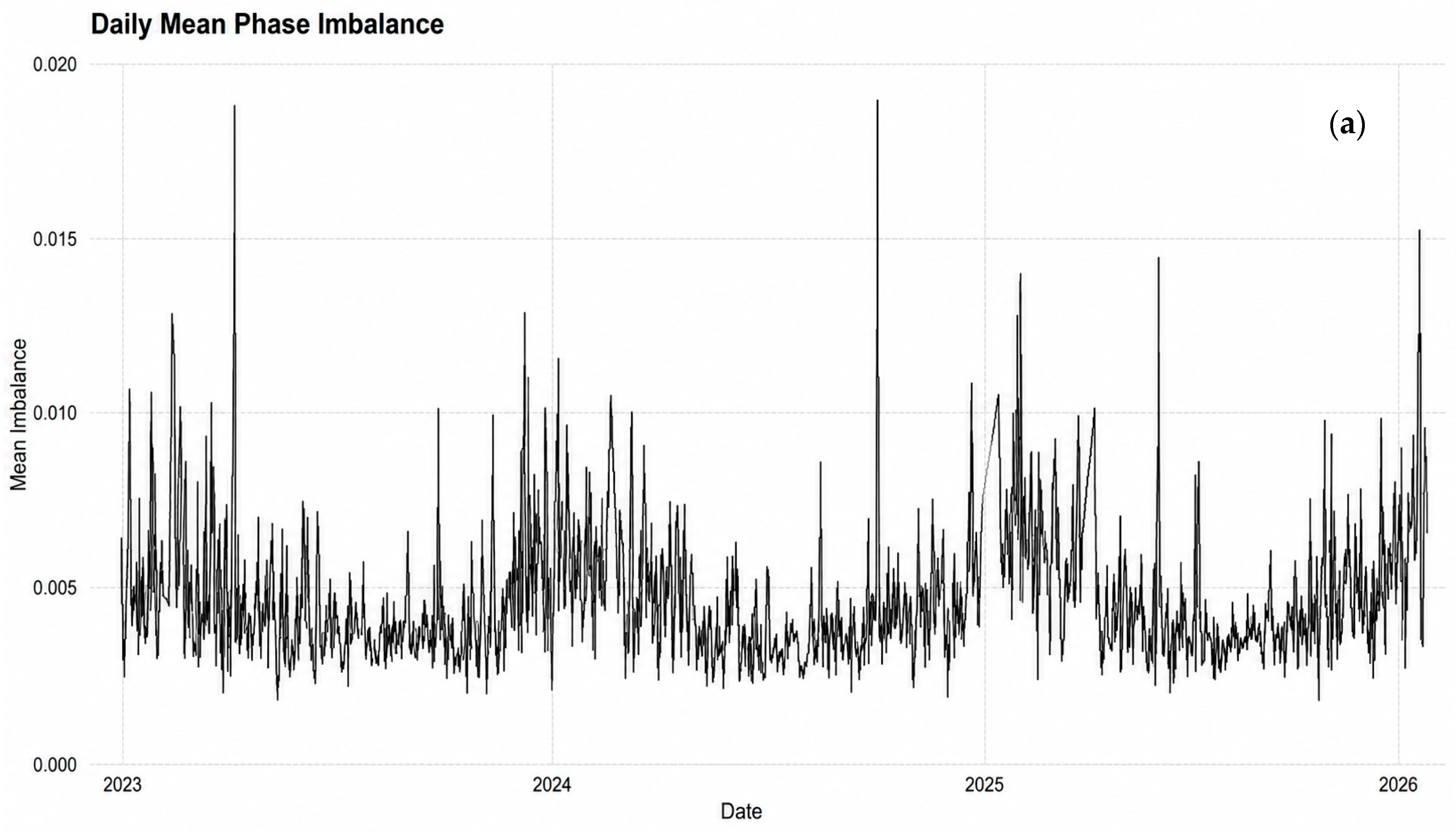
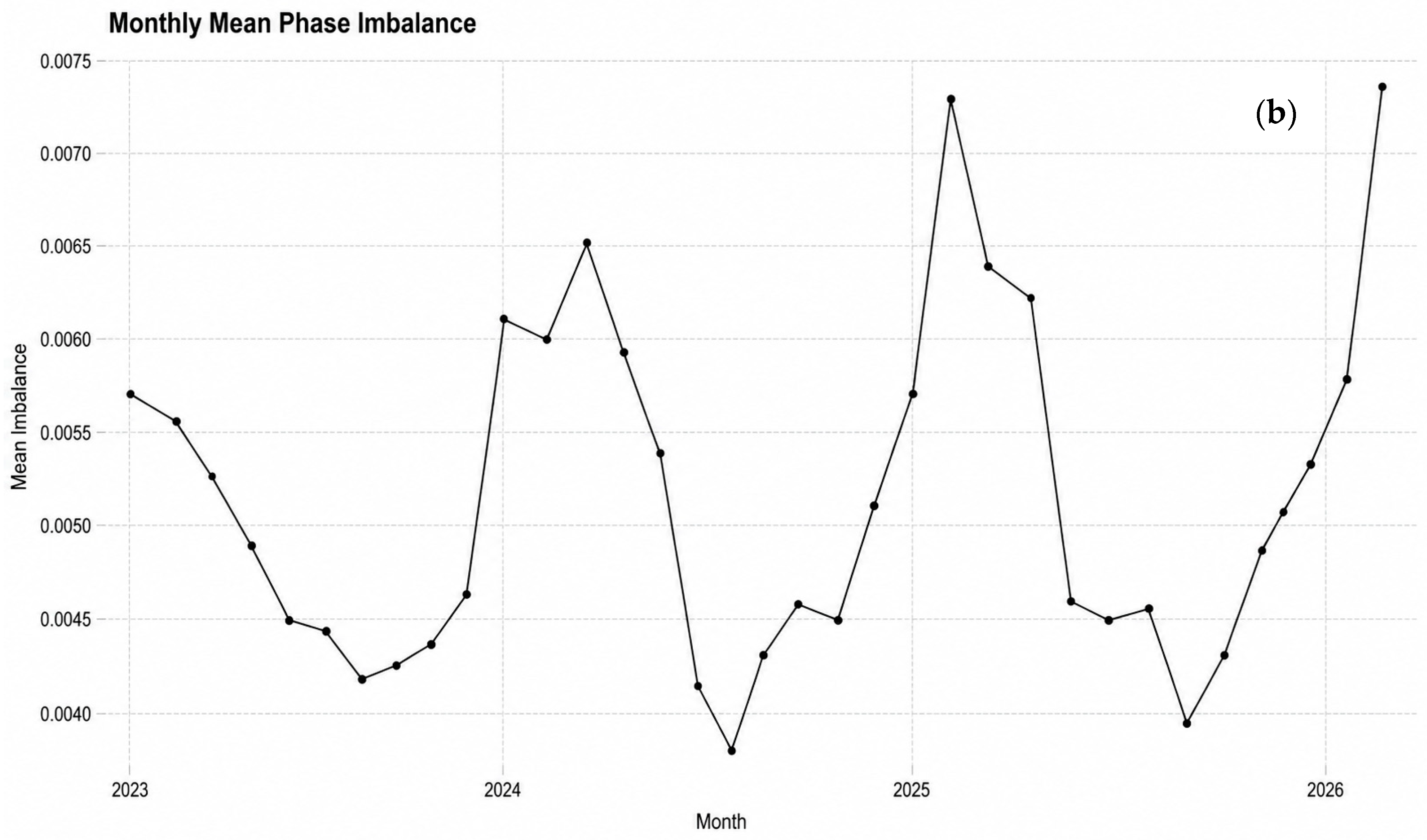
The temporal behavior of the Phase Imbalance Index is further illustrated in Figure 4. The daily imbalance series in the upper panel shows that most daily mean values remained at low levels, generally below 1%, confirming stable phase balance over time. Nevertheless, the daily pattern also reveals intermittent spikes, indicating that the system occasionally experienced short-lived increases in phase imbalance. These deviations were not persistent, but their occurrence suggests that phase balance may be temporarily affected by operating conditions, load variation, environmental changes, or short-duration electrical disturbances.

The monthly series in the lower panel provides a smoother view of the same behavior and reveals a clearer low-frequency temporal pattern. Monthly mean imbalance values remained within a narrow range, again supporting the conclusion that the PV system preserved a high degree of phase symmetry during the study period. However, the monthly profile does not appear completely random. Relatively higher imbalance levels are visible toward the final months of some years and around transition periods between annual cycles. This indicates that phase imbalance may be influenced by seasonal or operational conditions, even though the magnitude of these changes remains small.

Importantly, Figure 4 does not indicate a sustained monotonic increase in phase imbalance over the observation period. Instead, the system exhibits low baseline imbalance with temporary peaks and clustered fluctuations. This distinction is important from an electrical health perspective. A persistent upward trend could suggest progressive deterioration or worsening phase asymmetry, whereas the observed pattern is more consistent with temporary operating effects superimposed on an otherwise stable three-phase structure.

Overall, the descriptive statistics and temporal imbalance profiles provide consistent evidence that the photovoltaic system maintained stable and balanced three-phase operation during most active generation periods. At the same time, the presence of occasional imbalance spikes suggests that the Phase Imbalance Index remains useful as an operational monitoring variable. Even when the average imbalance level is low, localized deviations may contain relevant diagnostic information and may help identify operating periods in which electrical stability, power generation, or conversion efficiency could be affected. Having established that the system generally operated under balanced three-phase conditions, the next step is to examine whether variations in phase imbalance are associated with production performance and conversion efficiency.

4.4. Association Between Phase Imbalance and Active Power Generation Performance

The following analysis investigates the relationship between the Phase Imbalance Index and total active power generation, and subsequently evaluates its contribution to efficiency dynamics together with current- and voltage-related indicators. A moderate negative association was observed between the phase imbalance index and total active power generation ($\rho$ = −0.35), indicating that higher levels of phase imbalance tend to coincide with lower electricity production. In other words, an increase in phase imbalance appears to be associated with a reduction in power output. However, visual inspection of the scatter distribution suggests that this relationship may not be strictly linear, implying that the impact of phase imbalance on system performance may not be adequately captured by a simple linear model. Although the phase imbalance index does not appear to be a strong explanatory variable for power generation, identifying the periods during which elevated imbalance levels occur remains important for assessing potential operational risks and maintaining system reliability.

PV system performance is governed by complex electrical processes in which the relationships between operational variables and conversion efficiency are often nonlinear. Conventional linear regression models assume a constant marginal effect of explanatory variables across the entire range of observations, which may not adequately represent the behavior of photovoltaic systems under varying operating conditions. In contrast, GAM allow predictor variables to be modeled through smooth, data-driven functions, enabling the detection of nonlinear patterns without imposing a predefined functional form [35]. Therefore, GAM was preferred in this study to investigate the potentially nonlinear effects of mean current, mean voltage, and phase imbalance on photovoltaic conversion efficiency and to provide a more flexible representation of the underlying electrical dynamics.

4.4.1. The Results of GAM Analysis

The results demonstrate a strong explanatory performance for photovoltaic conversion efficiency, with an adjusted R² value of 0.664 and a deviance explained of 66.4%. These values indicate that the selected electrical indicators account for a substantial proportion of the variability in system efficiency. The high explanatory power of the model suggests that efficiency dynamics can be effectively characterized using a combination of current, voltage, and phase imbalance measurements. Furthermore, the close agreement between the adjusted R² and deviance explained values indicates a stable model structure without evidence of substantial overfitting.

Examination of the smooth terms reveals in

Table 5. Significance and Nonlinear Effects of Electrical Predictors in the GAM.

Variable	EDF	F	p
Mean Current	8.96	1883	<0.001
Mean Voltage	1.27	4.96	0.026
Imbalance	8.54	12.78	<0.001

that mean current is the most influential predictor of efficiency (df = 8.963, F = 1883.114, p < 0.001). The relatively large effective degrees of freedom indicate a pronounced nonlinear relationship between current and conversion efficiency, confirming that efficiency changes cannot be adequately represented by a simple linear function. Similarly, the phase imbalance index also exhibits a statistically significant nonlinear effect on efficiency (df = 8.538, F = 12.783, p < 0.001), suggesting that even relatively small variations in phase balance contribute to efficiency fluctuations. In contrast, mean voltage shows only a weak but statistically significant influence (df = 1.276, F = 4.965, p = 0.0257). The effective degree of freedom close to one indicates that the voltage–efficiency relationship is largely linear and considerably less important than the effects associated with current and phase imbalance. Overall, the GAM results identify mean current as the dominant determinant of photovoltaic conversion efficiency, while phase imbalance acts as a secondary but meaningful factor influencing system performance. The nonlinear nature of both mean current and phase imbalance effects highlights the importance of flexible modeling approaches such as GAM for capturing complex operational behaviors in photovoltaic systems.

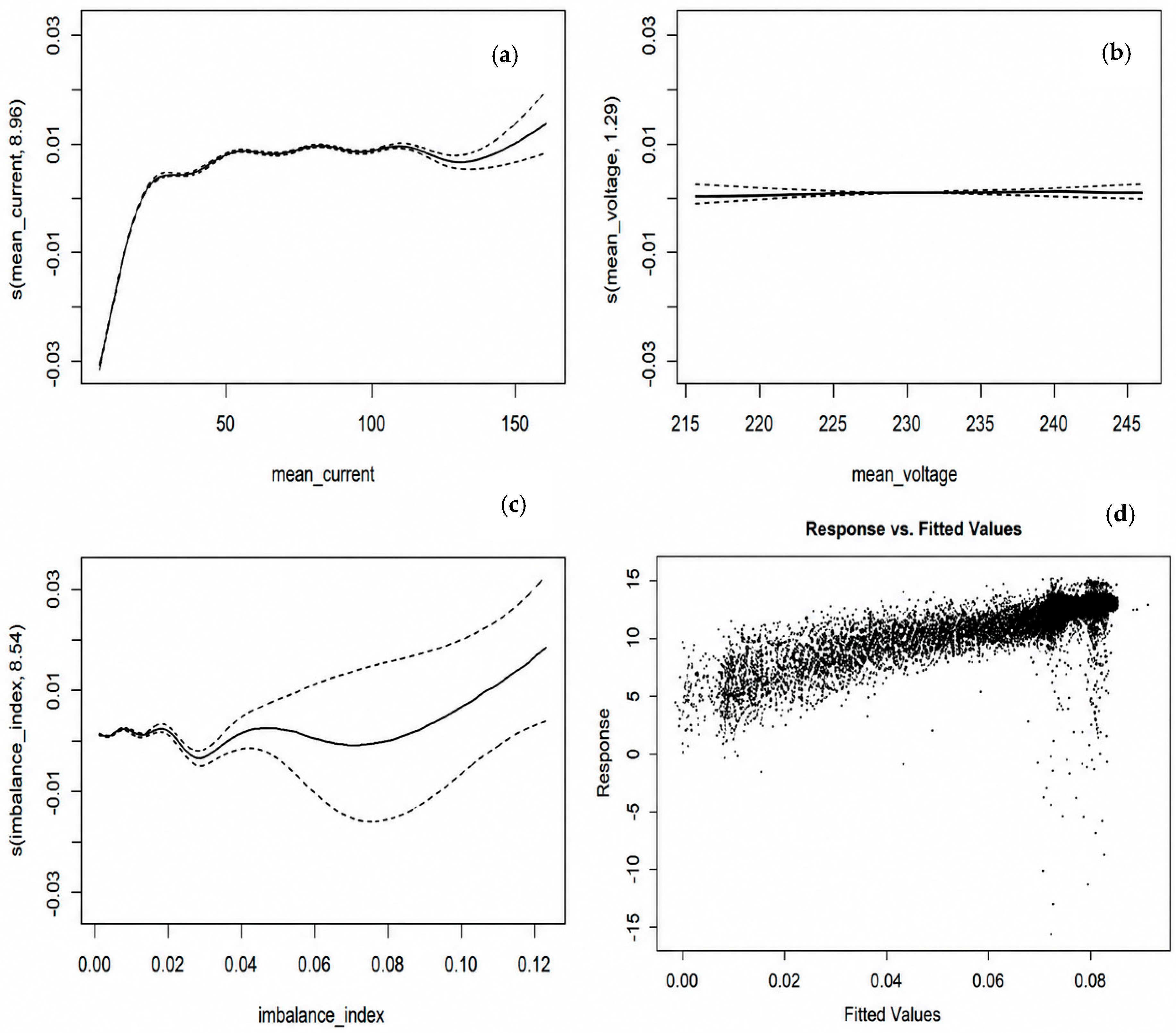
The partial effect plots obtained from the GAM revealed distinct nonlinear relationships between photovoltaic conversion efficiency and the examined electrical parameters. Mean current emerged as the most influential predictor, exhibiting a pronounced nonlinear effect characterized by rapid efficiency changes at lower current levels and a more stable pattern at moderate and high current ranges. In contrast, mean voltage showed only a limited contribution, with a nearly linear and relatively weak effect on efficiency. Although phase imbalance remained generally low throughout the study period, its effect was found to be statistically significant and nonlinear, indicating that variations in phase balance may influence system performance under certain operating conditions. Overall, the results demonstrate that GAM successfully captures complex operational relationships that cannot be adequately represented by conventional linear models.

The response-versus-fitted values plot (Figure 5) indicates that the GAM provides a satisfactory representation of photovoltaic conversion efficiency. Most observations are concentrated around the fitted values without exhibiting strong systematic patterns, suggesting an adequate model specification. Although a small number of observations deviate from the main distribution, particularly at higher efficiency levels, the overall structure confirms that the model captures the dominant variation in system performance. These findings are consistent with the relatively high explanatory power of the model (adjusted R² = 0.664), indicating that the selected electrical variables successfully explain a substantial proportion of efficiency variability.

Figure 5 illustrates the nonlinear relationships estimated by the Generalized Additive Model. The smooth effect of mean current shows the strongest pattern. At low current levels, the smooth function assumes negative values, indicating that low-current operating conditions are generally associated with lower photovoltaic conversion efficiency. As current increases, the effect rises rapidly and then stabilizes, suggesting that operation within higher current ranges generally corresponds to more efficient energy conversion. This behavior can be interpreted in light of the operating characteristics of photovoltaic systems and grid-connected inverters. Under normal operating conditions, the inverter maximum power point tracking (MPPT) algorithm continuously adjusts the operating point so that the PV array voltage remains within a relatively narrow range around the maximum power point, whereas the output current responds much more directly to variations in solar irradiance and other operating conditions. Consequently, disturbances such as partial shading, soiling, module mismatch, degradation, or transient weather conditions are generally reflected more strongly in the current than in the voltage. From the inverter perspective, low-current operating conditions are typically associated with reduced input power and partial-load operation, under which fixed internal losses constitute a larger proportion of the processed power. As a result, these operating conditions are generally associated with lower overall conversion efficiency. Therefore, mean current should not be interpreted as the physical cause of efficiency degradation; rather, it serves as an informative electrical indicator that reflects the combined effects of multiple operating conditions influencing PV system performance. Accordingly, the statistical relationship identified by the GAM is supported by the underlying operating characteristics of photovoltaic systems and grid-connected inverters. The effect of mean voltage is nearly flat across the observed voltage interval. Although statistically significant, its practical contribution to efficiency variation appears limited. This suggests that voltage remained relatively stable during operation and was not the main driver of efficiency changes. The effect of mean voltage is nearly flat across the observed voltage interval.

The phase imbalance index shows a weaker but nonlinear effect. At low imbalance levels, the effect is small, which is consistent with the generally balanced operation of the system. However, the curve becomes more variable at higher imbalance values, indicating that elevated imbalance may affect efficiency under specific operating conditions. The wider confidence intervals in this region suggest greater uncertainty, likely due to the limited number of high-imbalance observations. The response-versus-fitted plot indicates that the GAM captures the main structure of conversion efficiency reasonably well. Most observations follow the fitted pattern, although some lower-efficiency deviations remain. These deviations support the need for additional risk-detection analysis to identify low-efficiency operating episodes more explicitly.

To evaluate the stability of photovoltaic conversion performance, conversion efficiency was summarized at three temporal aggregation levels: instantaneous, daily, and monthly. This comparison allows short-term fluctuations to be distinguished from more persistent efficiency patterns. While instantaneous values reflect high-frequency operational variability, daily and monthly averages provide a clearer indication of the system’s sustained conversion performance over time.

As shown in

Table 6. Descriptive statistics of photovoltaic conversion efficiency at different temporal aggregation levels.

Statistic	Instantaneous Efficiency	Daily Mean Efficiency	Monthly Mean Efficiency
Minimum	0.788	0.910	0.948
1st Quartile	0.960	0.959	0.959
Median	0.969	0.964	0.963
Mean	0.964	0.962	0.962
3rd Quartile	0.972	0.968	0.967
Maximum	0.987	0.973	0.970

, the photovoltaic system exhibited consistently high conversion efficiency throughout the observation period. At the instantaneous level, the mean efficiency was 0.964, while the median was 0.969, indicating that most operating periods were characterized by effective DC-to-AC conversion. The narrow interquartile range, from 0.960 to 0.972, further suggests that efficiency values were concentrated within a stable high-performance interval.

The minimum instantaneous efficiency value of 0.788 indicates the presence of occasional low-efficiency observations. However, these deviations appear to be short-lived rather than persistent, as the minimum efficiency increased to 0.910 at the daily level and 0.948 at the monthly level. This pattern shows that temporal aggregation substantially reduces the effect of isolated low-efficiency events.

Daily and monthly efficiency values remained highly stable. Monthly mean efficiency was 0.962, with values ranging only from 0.948 to 0.970. The close agreement between the mean and median values across all aggregation levels indicates that the efficiency distribution was not strongly skewed by prolonged low-performance periods. Taken together, these results suggest that the PV system maintained stable conversion performance over time, with only occasional transient efficiency losses and no descriptive evidence of persistent low-efficiency operation.

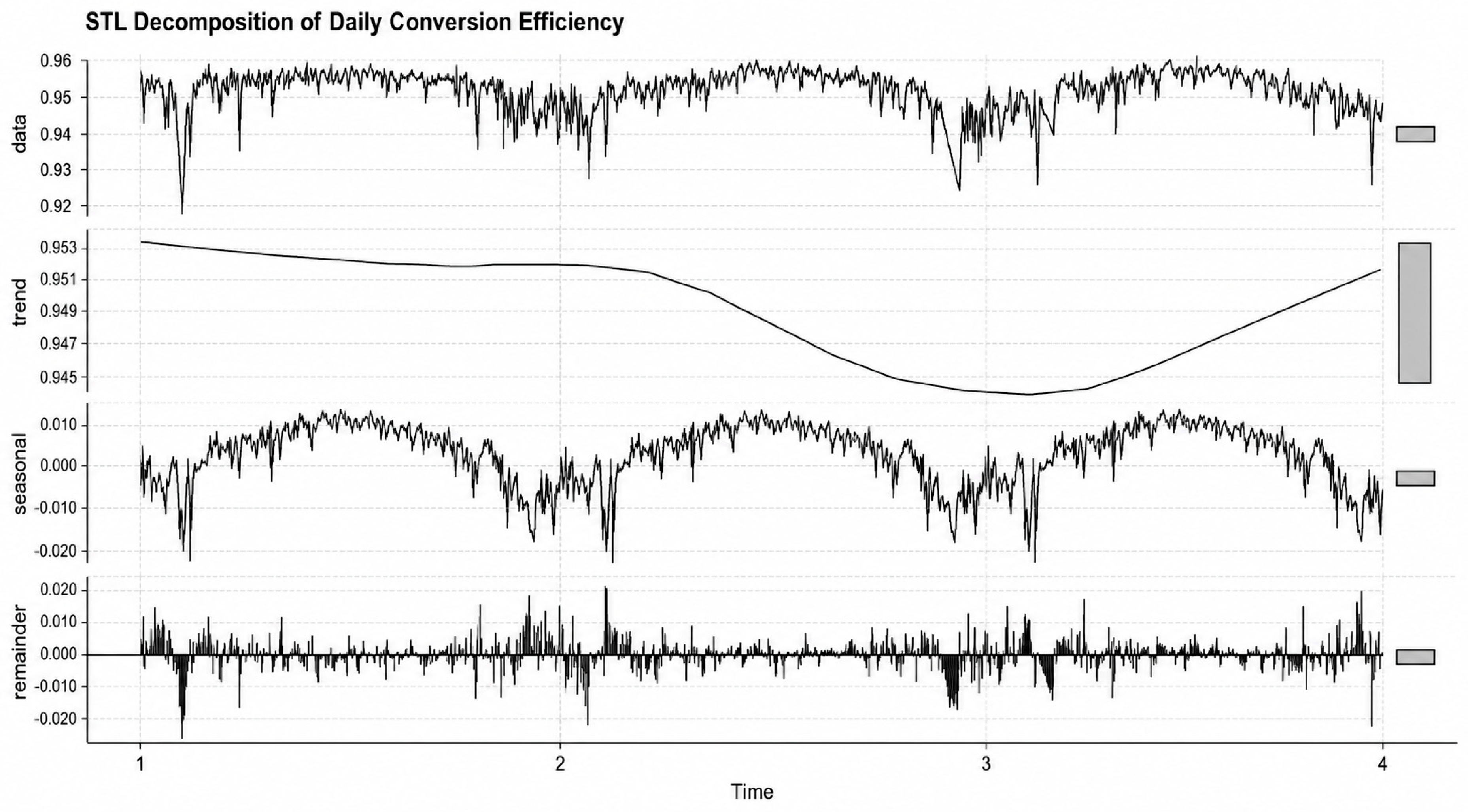
To further examine the temporal behavior of photovoltaic conversion efficiency, STL decomposition was applied to the daily efficiency series. This analysis allows the observed efficiency pattern to be decomposed into three components: a long-term trend, a recurring seasonal component, and an irregular remainder. In this way, temporary fluctuations can be distinguished from systematic seasonal variation and potential long-term performance changes. As shown in Figure 6, the observed daily efficiency series remained generally stable, although several short-term downward deviations were visible during the study period. The trend component reveals a moderate decline during the middle of the observation window, followed by a gradual recovery toward the end of the period. This pattern suggests that the system did not experience a continuous or irreversible loss of conversion performance. Instead, the mid-period reduction appears to reflect temporary operating conditions rather than persistent degradation.

The seasonal component shows a clear and recurring annual structure, indicating that conversion efficiency was influenced by seasonal operating conditions. This is consistent with the expected behavior of PV systems, where changes in solar availability, environmental conditions, and seasonal operating regimes may affect conversion performance. The presence of this seasonal pattern also confirms that efficiency should not be interpreted as a purely stationary variable over time.

The remainder component remains mostly centered on zero and does not display a strong systematic pattern. This indicates that the STL decomposition successfully captured the dominant trend and seasonal dynamics in the daily efficiency series. However, the presence of several isolated residual spikes suggests that occasional short-term disturbances or atypical operating conditions still affected efficiency on specific days.

The STL results should be interpreted together with the formal trend analysis. The Mann–Kendall test identified a weak but statistically significant negative trend in daily efficiency, with τ = −0.1206 and p = 5.16 × 10⁻⁹, while Sen’s slope was extremely small at −0.000004. Therefore, although a slight downward tendency can be detected statistically, its practical magnitude is limited. In combination with the STL decomposition, these findings suggest minor long-term efficiency variation rather than substantial performance degradation. The system therefore maintained relatively stable conversion performance, with predictable seasonal fluctuations and occasional short-term low-efficiency deviations.

4.4.2. The Results of Efficiency Analysis

To better understand the operating conditions associated with different efficiency states, the analysis was extended from aggregate efficiency statistics to episode-based and regime-based comparisons. This step provides a more operational interpretation of conversion efficiency by examining whether low- efficiency, normal- efficiency, and high-efficiency periods are associated with distinct current levels. Since previous analyses indicated that mean current was the dominant determinant of efficiency, this comparison helps clarify whether low-efficiency behavior is primarily linked to low-loading conditions.

As shown in

Table 7. Efficiency Episode and Efficiency Regime Statistics.

Episode	Mean Efficiency	Mean Current
Low Efficiency	0.923	13.7 A
Normal Efficiency	0.966	50.4 A
High Efficiency	0.977	62.4 A
Regime	Mean Efficiency	Mean Current
Low Regime	0.950	21.0 A
Medium Regime	0.969	53.1 A
High Regime	0.973	73.5 A

, low-efficiency episodes were characterized by a substantially lower mean current than normal- and high-efficiency episodes. The mean current during low-efficiency episodes was only 13.7 A, whereas normal-efficiency and high-efficiency episodes were associated with mean current levels of 50.4 A and 62.4 A, respectively. This contrast indicates that reduced conversion efficiency occurred predominantly under low-current operating conditions. In terms of efficiency values, the low-efficiency group had a mean efficiency of 0.923, compared with 0.966 in the normal-efficiency group and 0.977 in the high-efficiency group. The regime-based analysis in Table 7 confirms the same pattern. Mean current increased monotonically from 21.0 A in the low-efficiency regime to 53.1 A in the medium-efficiency regime and 73.5 A in the high-efficiency regime. This progressive increase demonstrates that the efficiency regimes are strongly differentiated by operating current levels. In contrast, the difference in mean efficiency between the medium- and high-efficiency regimes was relatively small, increasing from 0.969 to 0.973, which suggests that after the system reaches a sufficient current range, additional current increases produce more limited efficiency gains.

These findings are consistent with the GAM results, which identified mean current as the dominant nonlinear predictor of conversion efficiency. They also provide a clear operational interpretation: low-efficiency behavior is mainly associated with low-current, low-loading conditions rather than a persistent system-wide degradation process. Therefore, mean current can be considered a key diagnostic variable for distinguishing unfavorable operating states from normal and high-performance conditions. Notably, the average current observed during high-efficiency episodes was approximately 4.5 times greater than that observed during low-efficiency episodes. This substantial difference further emphasizes the dominant role of operating current in governing photovoltaic conversion efficiency.

This episode-based and regime-based evidence also provides the basis for the subsequent early-warning analysis. Since low-efficiency periods are strongly concentrated under low-current conditions, machine learning models and decision rules can use current-related thresholds, together with phase imbalance indicators, to identify operating states with elevated low-efficiency risk.

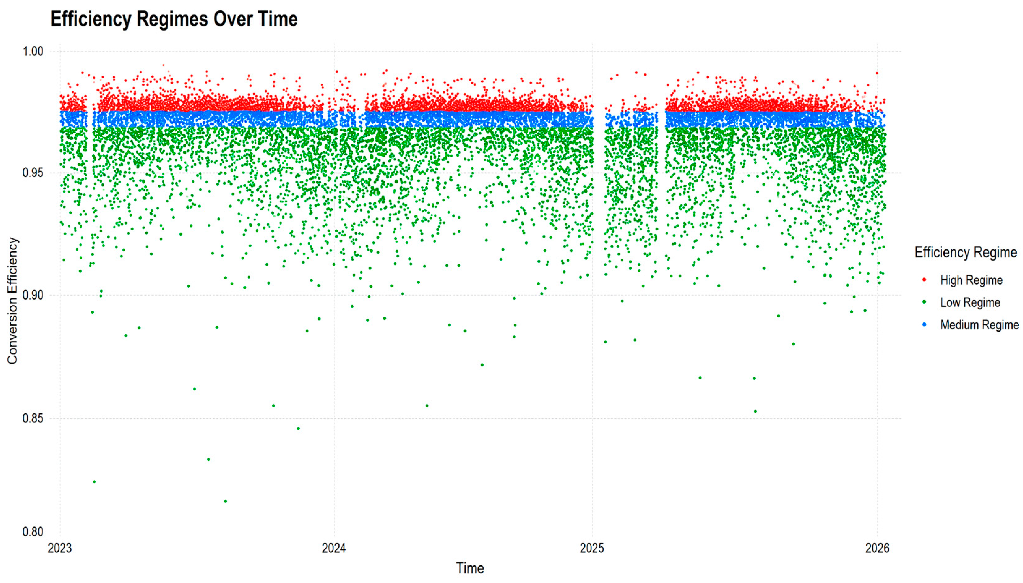
Figure 7 shows the temporal distribution of low-, medium-, and high-efficiency regimes over the study period. Medium-efficiency and high-efficiency observations form relatively stable bands around the upper efficiency range, indicating that the PV system generally maintained consistent conversion performance. Low-efficiency observations appear intermittently across the period and show greater downward dispersion, suggesting that reduced efficiency occurred mainly as short-term episodes rather than as a persistent degradation pattern. The absence of a sustained downward shift in the regime structure supports the conclusion that the system remained operationally stable over time.

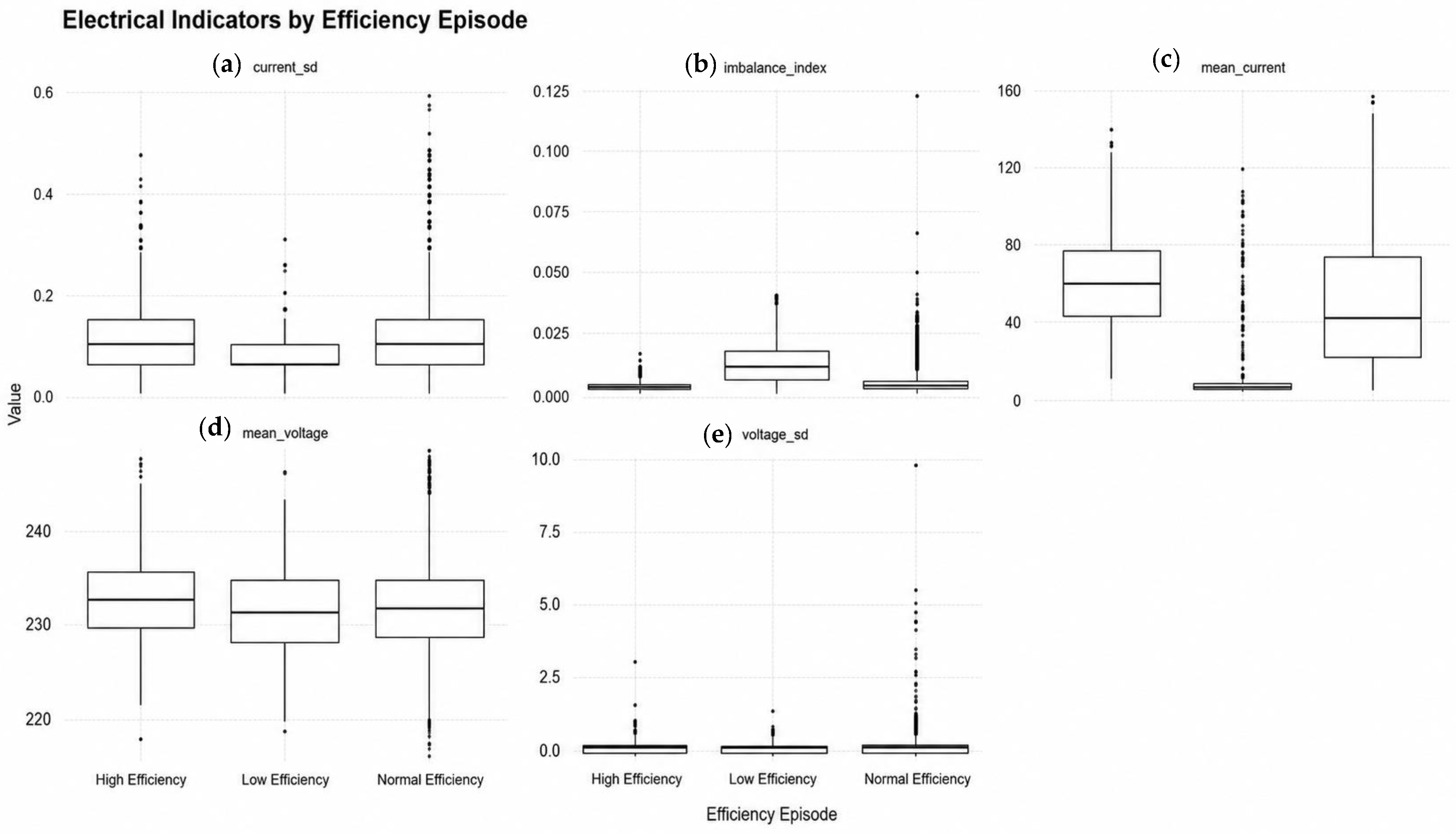
Figure 8 compares the distributions of key electrical indicators across low-efficiency, normal-efficiency, and high-efficiency episodes. The most distinct separation is observed for mean current, where low-efficiency episodes are concentrated at substantially lower current levels, confirming that reduced efficiency is mainly associated with low-loading operating conditions. The phase imbalance index is also higher and more dispersed during low-efficiency episodes, suggesting that phase asymmetry may intensify efficiency losses under unfavorable operating states. In contrast, mean voltage remains relatively similar across efficiency groups, while current and voltage variability show several outliers but weaker group separation. These patterns indicate that efficiency episodes are primarily differentiated by current-related behavior and, secondarily, by phase imbalance rather than voltage instability. As a result, the findings suggest that photovoltaic conversion efficiency is mainly governed by loading conditions, while phase imbalance acts as a secondary performance determinant. In other words, Efficiency regimes are primarily differentiated by operating current levels and, to a lesser extent, by phase imbalance conditions, whereas voltage-related indicators remain relatively stable across regimes.

4.4.3. Early-Warning Detection of Low-Efficiency Operating Conditions

Building on the evidence that low-efficiency episodes are mainly associated with low-current operating conditions and, to a lesser extent, elevated phase imbalance, this section evaluates whether such events can be detected in advance using high-frequency inverter-based electrical measurements. For this purpose, a Random Forest classifier was developed to estimate the probability of low-efficiency operation, and decision-tree-based threshold rules were subsequently derived to translate the model outputs into interpretable early-warning indicators for PV system monitoring. The Random Forest model (

Table 8. Random Forest Classification Performance for Low-Efficiency Event Detection.

Metric	Value
Total Observations	20,108
Low-Efficiency Observations	1006 (5.0%)
Normal-Efficiency Observations	19,102 (95.0%)
Number of Trees	500
Out-of-Bag (OOB) Error	3.87%
Overall Accuracy	96.34%
True Positives (Low Efficiency Correctly Identified)	156
False Negatives (Missed Low-Efficiency Events)	136
False Positives (False Alarms)	85
Recall for Low-Efficiency Events	53.4%

) demonstrated strong predictive performance in identifying low-efficiency events, achieving an overall classification accuracy of 96.34% with an out-of-bag error rate of only 3.87%. Low-efficiency events were defined as observations with inverter conversion efficiency values at or below the 5th percentile threshold estimated from the training dataset. Accordingly, only 5% of the observations were assigned to the low-efficiency class. Although the dataset exhibited a highly imbalanced structure, with low-efficiency observations representing only 5% of all records, the model successfully detected approximately 53% of low-efficiency events while maintaining a relatively low false-alarm rate. These results indicate that the proposed framework can identify a substantial proportion of efficiency losses without generating excessive operational warnings.

The moderate recall of 53.4% for low-efficiency events is likely associated with the pronounced class imbalance, as low-efficiency observations constitute only a small fraction of the available data. Under such conditions, the impurity-based splitting and majority-voting mechanisms of a standard Random Forest may favor the dominant normal-operation class, thereby increasing the number of false-negative predictions. In addition, observations close to the low-efficiency threshold may exhibit electrical characteristics that overlap with those of normal operating periods, making the minority class more difficult to distinguish. Consequently, some low-efficiency events were classified as normal despite the high overall accuracy. Therefore, model performance should be interpreted by considering minority-class recall and F1-score together with overall accuracy. Future improvements may include class-weighted learning, balanced sampling, cost-sensitive classification, and decision-threshold optimization to reduce missed low-efficiency events.

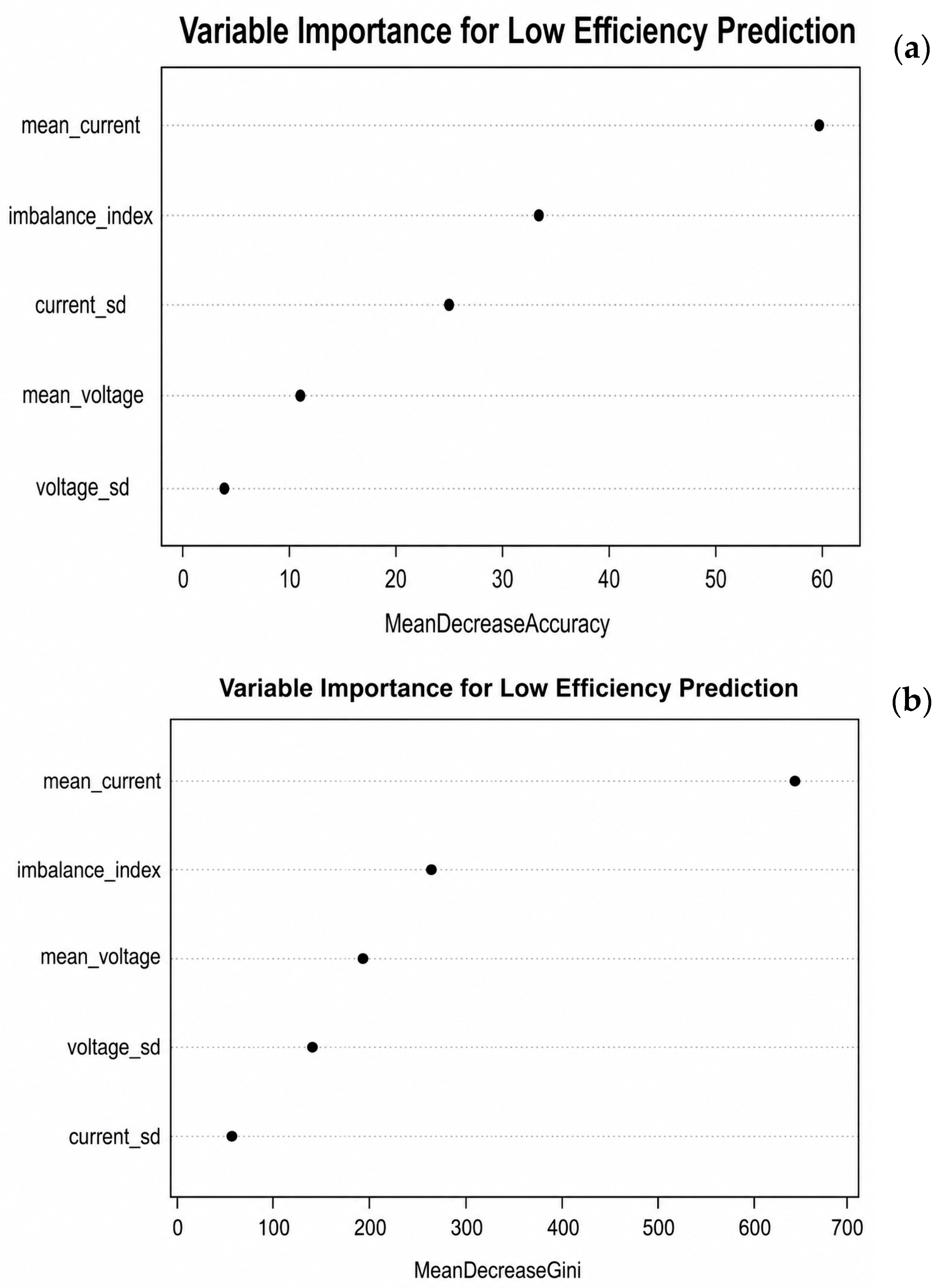
The variable importance analysis (

Table 9. Variable Importance Measures from the Random Forest Model.

Variable	Mean Decrease Accuracy	Mean Decrease Gini
Mean Current	60.17	617.72
Imbalance Index	33.19	250.40
Current SD	25.92	70.75
Mean Voltage	9.41	200.17
Voltage SD	4.14	158.25

) revealed that mean current was by far the most influential predictor of low-efficiency events, substantially outperforming all other electrical indicators in both Mean Decrease Accuracy and Mean Decrease Gini measures.

To assess the extent to which Random Forest performance depended on mean current, an ablation analysis was performed by retraining the model after excluding this variable while retaining the same chronological data partition and modeling configuration. The detailed results of this analysis are presented in Appendix A (

Table A1. Random Forest ablation analysis assessing the contribution of mean current.

Model	Accuracy	Recall	Precision	F1
Full RF	96.15	46.73	71.09	56.39
RF without Mean Current	95.67	34.27	68.75	45.74
Change (percentage points)	−0.48	−12.46	−2.34	−10.65

). Removing mean current reduced recall from 46.73% to 34.27% and the F1-score from 56.39% to 45.74%, corresponding to decreases of 12.46 and 10.65 percentage points, respectively. Precision decreased from 71.09% to 68.75%, whereas accuracy changed only marginally from 96.15% to 95.67%. Because low-efficiency events constitute the minority class, the reductions in recall and F1-score are more informative than the limited change in overall accuracy. These findings confirm that mean current is the dominant predictor, while the remaining electrical indicators retain meaningful predictive information.

This finding is consistent with the GAM, efficiency regime, and episode analyses, all of which identified current-related operating conditions as the primary determinant of photovoltaic conversion efficiency. Notably, the phase imbalance index emerged as the second most important predictor despite its generally low magnitude throughout the study period. This result suggests that even small deviations from phase balance may contribute to efficiency losses under certain operating conditions. In contrast, voltage-related indicators exhibited comparatively weaker explanatory power.

Taken together, the classification and variable importance results show that low-efficiency events can be partially detected from inverter-based electrical measurements, with mean current emerging as the dominant risk indicator and phase imbalance providing additional diagnostic value under unfavorable operating conditions.

Figure 9 presents the variable importance measures obtained from the Random Forest model. Mean current emerged as the most influential predictor of low-efficiency events according to both Mean Decrease Accuracy (60.17) and Mean Decrease Gini (617.72) metrics, indicating that loading conditions are the primary determinant of photovoltaic conversion efficiency. The phase imbalance index ranked as the second most important variable, outperforming voltage-related indicators despite its relatively low average magnitude throughout the study period. This finding suggests that even minor deviations from phase balance may contribute to efficiency losses under certain operating conditions. The consistency of these results with the GAM, efficiency episode, and regime analyses strengthens the evidence that current-related operating conditions and phase balance characteristics jointly govern the occurrence of low-efficiency events in photovoltaic systems. An important observation is that phase imbalance remained relatively low throughout the monitoring period, yet consistently emerged as a significant predictor across multiple analytical approaches. This finding suggests that even minor electrical asymmetries may contain valuable information for identifying efficiency-related operating risks.

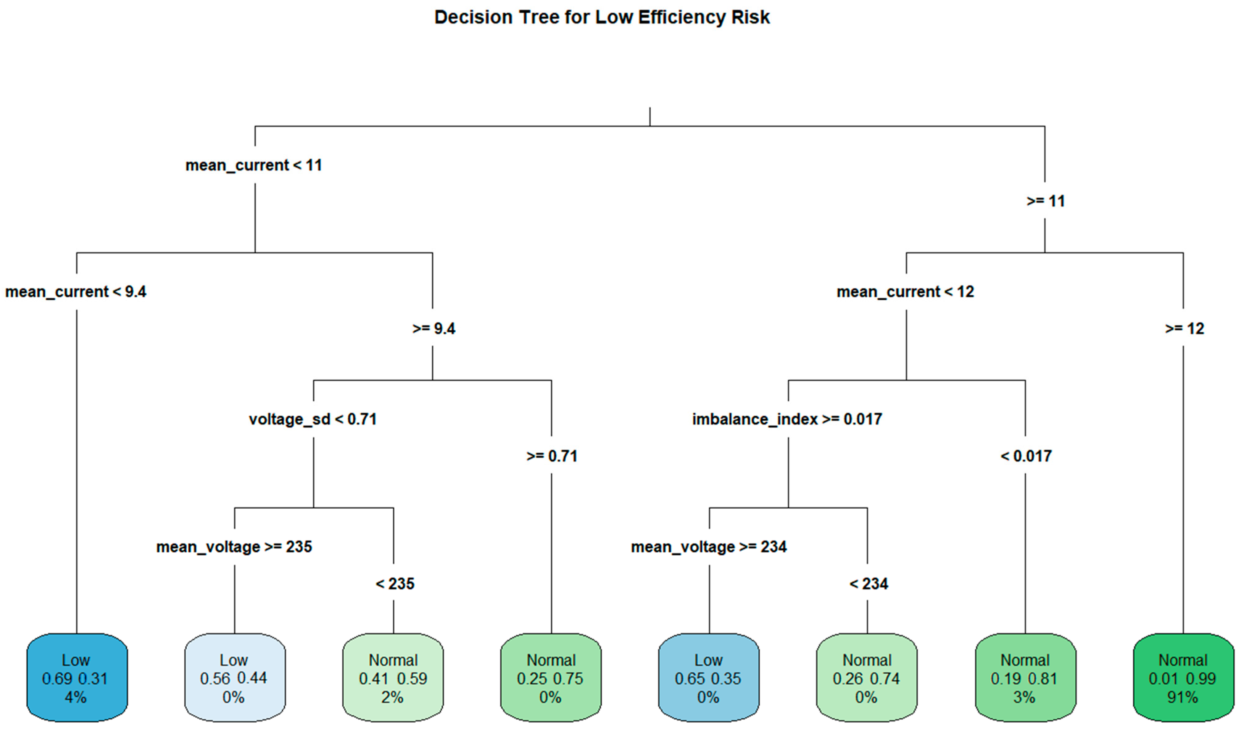
The decision tree analysis identified mean current as the primary operational threshold governing efficiency performance (Figure 10). Specifically, low-efficiency events became substantially more likely when mean current fell below approximately 10–11 A. Furthermore, phase imbalance emerged as a secondary risk factor, particularly under low-current operating conditions, where imbalance levels above 0.017 were associated with a marked increase in low-efficiency probability. These findings suggest that simple threshold-based monitoring rules can be used as an effective early-warning framework for photovoltaic performance management.

Table 10. Decision-tree-based operational thresholds for low-efficiency risk classification.

Rule	Operating Condition	Probability of Low Efficiency	Risk Level
R1	Mean Current < 9.4 A	69.4%	High
R2	Mean Current between 9.4 A and 11 A	40.8–55.6%	Moderate
R3	Mean Current < 12 A and Imbalance Index ≥ 0.017	65.0%	High
R4	Mean Current < 12 A and Imbalance Index < 0.017	26.4%	Low–Moderate
R5	Mean Current ≥ 12 A	0.7%	Very Low
R6	Mean Current ≥ 12 A and stable phase balance	<1%	Normal Operating Region

translates the model-based findings into interpretable operational rules for low-efficiency risk classification. The decision rules show that mean current is the primary threshold variable governing low-efficiency risk. When mean current falls below 9.4 A, the probability of low-efficiency operation increases to 69.4%, corresponding to a high-risk condition. Similarly, when mean current remains between 9.4 A and 11 A, the system enters a moderate-risk region, with low-efficiency probabilities ranging from 40.8% to 55.6%.

The results also show that phase imbalance becomes particularly important under low-current operating conditions. When mean current is below 12 A and the Phase Imbalance Index is at least 0.017, the probability of low-efficiency operation increases to 65.0%, indicating a high-risk state. By contrast, when the current is below 12 A but phase imbalance remains lower than 0.017, the estimated risk decreases to 26.4%, suggesting a low-to-moderate risk condition. This confirms that phase imbalance does not act as the dominant risk factor on its own, but it can amplify low-efficiency risk when the system is already operating under unfavorable low-current conditions.

A clear normal operating region is also identified. When mean current is at least 12 A, the probability of low-efficiency operation decreases sharply to 0.7%, and under stable phase-balance conditions it remains below 1%. This threshold structure provides a practical early-warning logic: low current should be treated as the main warning signal, while elevated phase imbalance should be interpreted as an additional risk amplifier.

These decision rules provide an operationally interpretable end point for the proposed monitoring framework. The results demonstrate that high-frequency inverter-based electrical measurements can be transformed into actionable indicators for PV system health monitoring, efficiency assessment, and early detection of low-efficiency operating conditions. In this respect, the proposed framework moves beyond descriptive performance evaluation and provides a practical decision-support structure for proactive maintenance and improved photovoltaic system reliability. Across the GAM, efficiency episode analysis, efficiency regime analysis, Random Forest classification, and decision-tree modeling, mean current consistently emerged as the dominant determinant of photovoltaic conversion efficiency. The remarkable agreement among these independent analytical approaches strengthens confidence in the proposed framework and indicates that current-related loading conditions represent the primary mechanism governing efficiency variation in the examined photovoltaic system.

5. Discussion

The findings of this study show that high-frequency inverter-based electrical measurements can provide meaningful information for both photovoltaic system health assessment and early detection of low-efficiency operating conditions. The correlation and phase imbalance analyses indicated that the examined PV system maintained a highly synchronized and electrically balanced three-phase structure during most active generation periods. However, the presence of occasional imbalance spikes also showed that global correlation analysis alone is not sufficient for operational monitoring. This supports the use of additional electrical condition indicators, such as the Phase Imbalance Index, to detect localized and time-dependent deviations that may not be visible from average power or voltage profiles alone.

The results also indicate that photovoltaic conversion efficiency is primarily governed by current-dependent operating conditions. This finding was consistent across the GAM, efficiency episode analysis, efficiency regime comparison, and Random Forest variable importance results. In particular, low-efficiency episodes were concentrated under low-current conditions, whereas voltage-related indicators remained comparatively stable across efficiency groups. This suggests that, for the monitored system, reduced efficiency was more closely related to loading conditions than to voltage instability. The nonlinear effect of mean current identified by the GAM further confirms that the current–efficiency relationship cannot be adequately represented by a simple linear model.

These findings are consistent with the broader PV monitoring literature, which emphasizes that electrical variables contain valuable diagnostic information about system performance and fault-related behavior [9,10]. However, the proposed framework differs from many previous studies in its objective and practical implementation. Several recent studies have reported very high classification performance using advanced machine learning, deep learning, image-based diagnostics, transfer learning, or hybrid architectures for specific PV fault types, such as open-circuit faults, short-circuit faults, partial shading, module degradation, hot spots, and high-impedance faults [17,19,26]. While these approaches provide strong diagnostic accuracy, many of them require image data, irradiance and temperature measurements, additional sensors, laboratory-based fault labels, or complex deep learning structures.

In contrast, the present study focuses on the early detection of low-efficiency operating conditions rather than the classification of predefined physical fault types. This distinction is important from an operational perspective. In real PV plants, different physical problems such as shading, soiling, mismatch, inverter-side irregularities, and electrical imbalance may produce similar performance symptoms, especially reduced power output and lower conversion efficiency [4,5,6,7,8]. Therefore, detecting harmful operating states before they evolve into persistent efficiency loss can be as valuable as identifying the exact fault mechanism. The proposed framework addresses this need by using only routinely available inverter measurements and by converting model outputs into interpretable risk rules. Accordingly, the practical value of the proposed framework lies in providing an early indication that system performance is deviating from its normal operating behaviour, thereby prompting timely inspection rather than identifying the exact physical cause of the deviation. Compared with deep learning-based PV fault diagnosis models, the proposed framework was designed to balance predictive performance, interpretability, and deployment simplicity. Deep learning architectures can automatically learn complex nonlinear and temporal representations from raw or high-frequency measurements and may achieve higher classification performance when sufficiently large, well-labelled datasets and adequate computational resources are available. However, these potential performance gains are generally accompanied by higher data requirements, greater computational cost, more extensive hyper-parameter tuning, and less transparent decision mechanisms. In contrast, the proposed framework provides different levels of interpretability: the GAM reveals the nonlinear effects of individual electrical indicators, the Random Forest captures interactions among these indicators, and the Decision Tree translates the dominant patterns into explicit operating thresholds. This structure facilitates the interpretation of low-efficiency warnings in terms of physically meaningful inverter operating conditions and supports their translation into maintenance decisions. Nevertheless, the use of engineered electrical indicators and conventional machine-learning models may provide less flexibility for identifying subtle temporal patterns than deep learning architectures, as reflected by the moderate recall of 53.4% for rare low-efficiency events. Therefore, the proposed framework is not claimed to universally outperform deep learning models in predictive accuracy; rather, it provides a practical trade-off among predictive performance, model interpretability, data requirements, computational burden, and field deployability. Because no deep learning model was evaluated using the same chronological data partition in this study, a direct quantitative comparison of prediction accuracy remains beyond the present scope.

The Random Forest results demonstrated that low-efficiency events can be partially detected from electrical indicators, with an overall accuracy of 96.34% and a recall of 53.4% for rare low-efficiency observations. This recall value is lower than the very high accuracies reported in some controlled fault classification studies [17,22,24], but the comparison should be interpreted carefully. The present problem is more operationally challenging because low-efficiency events are rare, imbalanced, and not necessarily associated with a single well-defined fault label. Therefore, the contribution of the model lies not only in classification performance but also in its ability to identify risk-relevant operating conditions and support practical early-warning decisions.

The decision-tree-based thresholds provide the most directly actionable output of the framework. Mean current below approximately 9.4 A was associated with a high probability of low-efficiency operation, while mean current above 12 A corresponded to a very low-risk operating region. Phase imbalance acted as a secondary risk amplifier, particularly under low-current conditions. This result is operationally important because it transforms complex model behavior into simple monitoring rules that can be interpreted by plant operators without requiring advanced machine learning expertise. In this respect, the proposed approach contributes to the literature by linking data-driven modelling with explainable decision support.

Despite these contributions, several limitations define the scope of the present findings and motivate specific directions for future research. First, because the framework was developed and evaluated using data from a single PV plant, the identified current and phase-imbalance thresholds may reflect the installed inverter rating, plant configuration, local climatic conditions, and site-specific operating regime. External validation across PV plants with different capacities, inverter technologies, and climatic conditions is therefore required to determine whether these thresholds are transferable or require site-specific recalibration. Second, the deliberate exclusion of solar irradiance, temperature, and maintenance-related information supports sensor-minimal deployment but restricts the physical attribution of detected low-efficiency events. In particular, low-current and low-efficiency observations cannot be unambiguously distinguished as normal low-irradiance operation, shading, soiling, or inverter-side performance degradation. Future studies should therefore assess the incremental value of a limited set of environmental and maintenance variables while preserving the interpretability and low deployment cost of the framework. Third, because low-efficiency events were defined using the lower 5th percentile of the training-set efficiency distribution rather than independently verified physical fault labels, the model identifies statistically rare low-efficiency operating states but does not determine their underlying fault mechanisms. Linking detected events with inverter alarms, maintenance records, field inspections, and labelled fault episodes would improve diagnostic specificity. Future work should also compare fixed percentile-based thresholds with seasonally adaptive or operating-condition-dependent thresholds.

Fourth, model performance was evaluated using a single chronological 70/30 hold-out partition. Although this design preserves temporal order and reduces information leakage, it does not fully quantify performance variability across different seasons, years, or operating regimes. Repeated blocked time-series validation, rolling-origin evaluation, and prospective testing on later operational periods should therefore be used to assess temporal robustness and model drift. Fifth, the recall of 53.4% indicates that a substantial proportion of rare low-efficiency events remained undetected, most likely because of class imbalance and overlapping electrical characteristics near the decision boundary. Future studies should investigate class-weighted or balanced ensemble models, cost-sensitive learning, probability calibration, and decision-threshold optimization, with particular emphasis on false-negative costs and precision–recall performance rather than overall accuracy alone. Finally, because no deep learning model was evaluated using the same input variables and chronological data partition, the predictive-performance–interpretability trade-off could not be quantified directly. A controlled comparison with temporal deep learning architectures under an identical experimental configuration would provide a more objective assessment of this trade-off.

Overall, the results suggest that routine inverter-based electrical measurements can be transformed into practical indicators of PV system health, efficiency behavior, and low-efficiency risk. Compared with more complex fault diagnosis approaches, the proposed framework offers a simpler, interpretable, and operationally deployable alternative for continuous condition monitoring and proactive maintenance decision-making.

6. Conclusions

This study proposed an interpretable data-driven framework for monitoring photovoltaic system health and detecting low-efficiency operating conditions using high-frequency inverter-based electrical measurements. The results showed that the examined PV system generally maintained stable three-phase operation, low phase imbalance, and high conversion efficiency during active generation periods. Across the GAM, efficiency regime analysis, Random Forest model, and decision-tree rules, mean current emerged as the dominant predictor of conversion efficiency and low-efficiency risk of conversion efficiency and low-efficiency risk, while phase imbalance acted as a secondary but operationally relevant risk factor.

Unlike conventional photovoltaic monitoring studies that primarily rely on meteorological variables such as solar irradiance and temperature, the proposed framework utilizes only high-frequency electrical measurements obtained directly from the inverter. This enables the development of an interpretable and operationally practical early-warning system without requiring additional environmental sensors. The derived decision rules further show that complex model outputs can be translated into simple thresholds for proactive maintenance and real-time performance monitoring.

The limitations of the present study also define the next research steps. Because the framework was evaluated using data from a single PV plant, multi-site validation is required to assess the transferability of the identified operating thresholds across different inverter technologies, plant capacities, and climatic conditions. Because meteorological and maintenance-related variables were excluded, future studies should evaluate whether a limited set of contextual measurements can distinguish normal low-load operation from environmentally or technically induced efficiency loss while preserving interpretability. Since low-efficiency events were defined statistically rather than through verified physical fault labels, future work should link detected events with inverter alarms, maintenance records, and field inspections and compare fixed thresholds with seasonally adaptive alternatives. Finally, the use of a single chronological hold-out period and the moderate recall for rare low-efficiency events motivate rolling-origin validation, class-weighted learning, probability calibration, and decision-threshold optimization to improve temporal robustness and reduce missed events.

The present study is based on data from one photovoltaic power plant, but the proposed analytical framework is not limited to this power plant. The workflow includes machine learning, explainable AI and multi-criteria decision-making techniques based on operational variables routinely monitored; thus, it can be adapted to other grid-connected photovoltaic systems with proper local calibration. However, the importance of variables and decision thresholds could be dependent on climatic conditions, system configuration and operational characteristics. Hence, the proposed framework needs to be recalibrated before its direct application to other PV installations.