Risk Assessment of River-Channel Washout Disasters for Long-Distance Oil and Gas Pipelines Considering Storm-Induced Flood Scour Effects

Abstract

River-channel washout is one of the common geological hazards threatening the safety of long-distance oil and gas pipelines, particularly under storm-flood conditions, when pipeline sections crossing rivers and gullies are more susceptible to damage. Existing assessment methods for river-channel washout are effective for single river cross-sections or post-disaster field investigations; however, their application remains limited when dealing with long-distance pipeline systems characterized by numerous river- and gully-crossing sections and large spatial variability in upstream catchment conditions. To address this issue, this study investigates storm-flood discharge and scour-depth calculation methods suitable for river- and gully-crossing sections of long-distance oil and gas pipelines, and establishes a quantitative evaluation index system that considers river-channel washout susceptibility, pipeline vulnerability, and pipeline failure consequences. Based on investigation results of river-channel washout hazards along multiple pipeline systems, including the Zhongxian–Yichang section of the Zhongwu Pipeline, the Hubei–Hunan section of the Lanzhou–Zhengzhou–Changsha Pipeline, and the Phase I Jiangxi Natural Gas Pipeline Network, the hazard characteristics and influencing factors of river-channel washout affecting long-distance oil and gas pipelines are analyzed and summarized. The proposed method was applied to 19 river- and gully-crossing pipeline sections in the Phase I Jiangxi Natural Gas Pipeline Network under different rainfall intensities. The results show that, under light-to-moderate rainfall conditions, 15 sites were classified as relatively low risk and 4 sites as medium risk. Under both the 50-year and 100-year return-period rainstorm scenarios, 12 sites were classified as relatively low risk, 6 sites as medium risk, and 1 site as relatively high risk. The results also indicate that the risk probability of some sites increases with increasing rainfall intensity. Among them, Site No. 19 shows the highest risk probability, increasing from 0.0997 under light-to-moderate rainfall conditions to 0.1474 and 0.1488 under the 50-year and 100-year return-period rainstorm scenarios, respectively. The proposed method can provide a reference for meteorological risk assessment of river-channel washout hazards along long-distance oil and gas pipelines.

1. Introduction

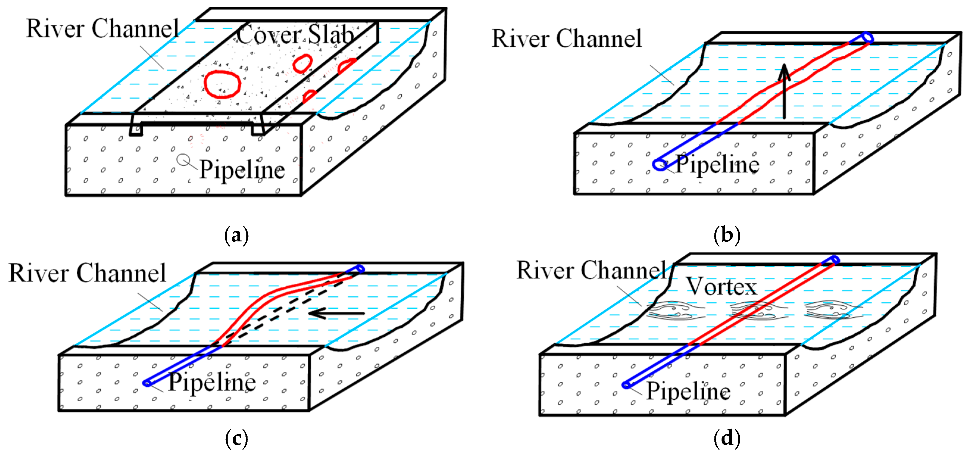
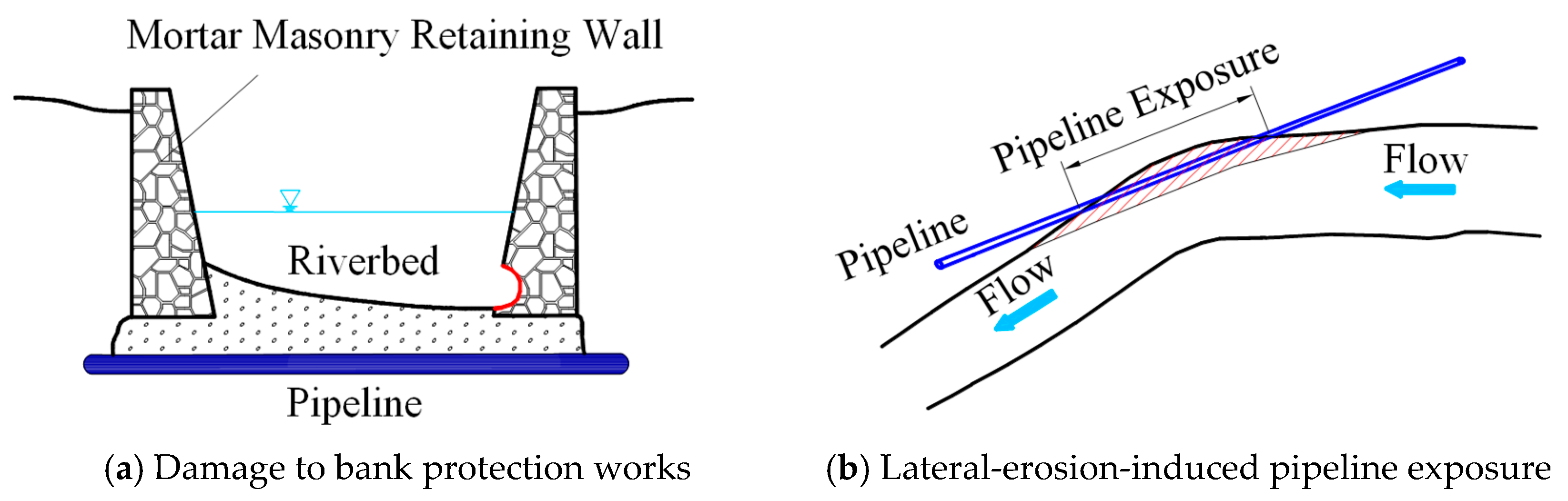
Long-distance oil and gas pipelines are an important component of energy transportation systems, and their routes commonly traverse various engineering geological units, such as mountainous areas, hills, plains, and river valleys. Influenced by geomorphology, soil and rock properties, meteorological and hydrological conditions, and human engineering activities, geological hazards along pipeline corridors are complex and diverse. Among them, river-channel washout is a type of hazard that is widely distributed, occurs frequently, and has a significant impact on pipeline safety. River-channel washout commonly occurs where pipelines cross rivers or gullies, or are laid along river channels. Under storm-flood conditions, river water level and flow velocity increase rapidly, and strong scouring, erosion, and downcutting of the riverbed and banks may occur. These processes can lead to thinning of pipeline cover, pipeline exposure, floating, free spanning, and damage to hydraulic protection structures. In severe cases, they may induce pipeline deformation, instability, or even failure [1,2,3,4,5]. Engineering practice has shown that river-channel washout does not necessarily manifest as sudden overall deformation in the same way as landslides or collapses. However, it is characterized by high occurrence frequency, strong concealment, clear dependence on rainfall processes, and high post-disaster treatment costs. Therefore, it is an important hazard type that cannot be ignored in geological hazard risk management for long-distance oil and gas pipelines [6,7,8].

Regarding river-channel washout and river scour, a relatively mature research foundation has been established both domestically and internationally. In terms of hydrological frequency analysis, the estimation of extreme rainfall and design floods is usually based on annual maximum series or peaks-over-threshold series. With the aid of extreme value theory, the Fisher–Tippett–Gnedenko theorem, and probability models such as the Gumbel distribution, generalized extreme value distribution, and Pearson Type III distribution, design rainfall or peak flood discharge under different return periods can be estimated [9,10,11,12,13,14]. In terms of river scour calculation, existing studies have considered factors such as flow velocity, discharge, water depth, riverbed composition, sediment particle size, bank-slope morphology, and protective structures, and have established local scour and general scour calculation methods applicable to bridges, levees, riverbank protection, and river-channel regulation projects [15,16,17]. These methods can effectively support the analysis of single river cross-sections, local engineering design, and post-disaster review, thereby providing an important hydrological and hydraulic basis for the risk assessment of river-channel washout hazards.

In terms of pipeline geological hazard risk assessment, the main approaches include qualitative evaluation, as well as the use of knowledge-driven and data-driven models to assess geological hazard susceptibility or risk. Knowledge-driven methods, such as geological hazard causation analysis, expert scoring, and the analytic hierarchy process, can fully incorporate engineering experience and are suitable for risk identification along pipeline corridors where data are insufficient or hazard types are complex [18,19,20]. Data-driven methods, such as the information value model, weights-of-evidence method, grey model, extension theory, and machine learning methods, can use existing investigation data to evaluate the hazard, vulnerability, and risk of regional or site-specific geological hazards [21,22,23,24]. Recent studies have also attempted to construct rapid safety assessment frameworks for long-distance oil and gas pipelines under geological hazard conditions by integrating susceptibility assessment, hazard assessment, risk evaluation, safety assessment, and multisource monitoring data [7]. In addition, regarding pipeline water-damage hazards, existing studies have analyzed aspects such as hazard modes, protective structures, pipeline floating stability, free-span safety, scour-depth calculation, and engineering prevention and control measures. These studies have indicated that river-channel washout mainly manifests as riverbed incision, bank lateral erosion, pipeline exposure, pipeline floating, free spanning, and failure of protective engineering works [25,26,27,28,29,30,31].

However, existing studies still have certain limitations when applied to the risk management of river-channel washout hazards along long-distance pipelines. Traditional hydrological frequency analysis and river-scour calculation mainly focus on the scour depth that may occur at a specific cross-section under a given flood condition, but they cannot directly reflect how the scour results affect the risk level of pipelines. Existing pipeline geological hazard risk assessment methods mostly rely on investigation indicators, expert experience, or statistical analysis of historical samples. Although these methods can be used for risk zoning and hazard-site ranking, they insufficiently consider the small-watershed rainfall–runoff process, flow-velocity variation, and scour-depth response induced by storm floods. Long-distance oil and gas pipelines usually include numerous river- and gully-crossing sections that are widely distributed. Different sites vary significantly in watershed area, channel slope, riverbed material, pipeline burial depth, installation mode, and protection conditions. Therefore, relying solely on post-disaster investigation or single-site engineering verification is insufficient to meet the needs of batch-based and scenario-based risk identification. Based on this understanding, this study does not aim to replace existing flood-frequency analysis or scour-calculation methods. Instead, it develops a quantitative risk assessment method for river-channel washout that considers storm-flood-induced scour effects and is oriented toward the operational management of long-distance oil and gas pipelines. The proposed method is based on small-watershed rainfall–runoff calculation under different rainfall return periods. It further estimates flow velocity, flow depth, and scour depth, and integrates indicators such as pipeline burial depth, protection conditions, installation mode, affected pipeline length, and failure consequences. In this way, a coupled risk assessment framework incorporating river-channel washout susceptibility, pipeline vulnerability, and failure consequences is established. Finally, typical river- and gully-crossing sections in the Phase I project of a natural gas pipeline network in Jiangxi Province are selected as case studies to conduct risk assessment and classification under different rainfall scenarios, providing a reference for dynamic identification, risk grading, and flood-season management of pipeline river-channel washout hazards.

2. Analysis of the Hazard Characteristics and Influencing Factors of River-Channel Washout Disasters

2.1. Modes of Action of River-Channel Washout Disasters on Pipelines

When long-distance oil and gas pipelines traverse rivers or gullies, they are commonly installed using methods such as open-cut installation, trenchless crossing, or floodplain laying. River-crossing sections often exhibit strong hydrodynamic forces, pronounced topographic relief, and loose geological materials. Under heavy rainfall conditions, large volumes of surface runoff can develop rapidly within the catchment area, causing a sharp increase in channel discharge. This results in significantly intensified scour, erosion, and undercutting effects. Under the influence of storm-flood events, pipelines and their associated hydraulic protection structures may undergo different forms of river-channel washout damage depending on the failure mechanisms involved. The main damage modes are vertical incision (Figure 1) and lateral erosion [32] (Figure 2).

Among these processes, the vertical incision of the riverbed is the main factor leading to damage of pipelines laid along river channels or installed by open-cut crossing through gullies, as well as their hydraulic protection works. Storm-flood events cause the vertical incision of the riverbed to intensify, and the channel base to be gradually incised and lowered. The riverbed downcutting may result in the foundations of hydraulic protection measures, such as bed protection, becoming shallower or being undermined (Figure 1a), thereby posing an indirect threat to the safe operation of the pipeline. Vertical incision may also cause the overburden above pipelines without protective measures to continuously thin, resulting in reduced burial depth or even pipeline exposure, thereby posing a direct threat to the safe operation of the pipeline. The main forms of damage caused by vertical incision to pipelines are as follows: insufficient overburden thickness above the pipeline, which leads to the formation of exposed sections and results in pipeline floating (Figure 1b). Under short-duration high-velocity flow scour, the pipeline continuously buckles and shifts downstream and upward (pipeline migration) (Figure 1c). Oil and gas pipelines that cross rivers using large-scale open-cut burial may develop unsupported spans that do not directly contact the riverbed surface. These suspended sections are subjected to flow-around effects, generating periodic vortex-induced vibrations (free span) [33] (Figure 1d).

Lateral erosion of river flow mainly refers to the susceptibility of concave banks at river bends to scouring and stripping by the water current. Under the action of storm-flood conditions, the river flow pattern changes, and due to centrifugal force, the flow velocity becomes highest along the concave bank and lower along the convex bank. Because the flow along the concave bank is faster and the shear stress is stronger, the bank is more prone to scouring, undercutting, and even collapse (Figure 2a). The lateral erosion of the river channel may undermine the foundations of retaining walls constructed to protect pipelines at the bank slopes. Once the foundation is eroded, the retaining wall loses support and subsequently collapses and fails. As erosion further progresses toward the interior of the floodplain, it may affect pipelines laid within the floodplain, resulting in lateral-erosion-induced pipeline exposure (Figure 2b), which can damage the coating or even the pipeline itself. Severe lateral erosion poses a significant threat to the safety of pipelines installed along the riverbank or crossing the riverbank.

2.2. Mechanisms of River-Channel Washout Under Storm-Flood Conditions

Rainfall causes changes in river discharge and flow velocity, and the increase in discharge and velocity leads to an increase in hydraulic energy, which in turn mobilizes soil and rock particles at the channel bed and banks, resulting in scour. Rainfall within a watershed, after deducting various forms of loss, enters the river network through surface and subsurface pathways. The process in which rainfall becomes effective rainfall after deducting various forms of loss is called the runoff-generation process. The effective rainfall then flows over hillslopes within the watershed, entering the river network through surface and subsurface pathways, and subsequently converges toward the watershed outlet section; this is referred to as the flow-convergence process. According to hydrological principles, the peak flood discharge in the river channel generated by the runoff-generation and flow-convergence processes can be quantitatively calculated. Based on this discharge, the corresponding flow depth and flow velocity for the given water volume can be obtained through hydraulic back-calculation, and the general scour depth of the river cross-section caused by a single storm-flood event can ultimately be computed.

Based on the above fundamental principles, exploring a quantitative risk-assessment method suitable for river-channel washout affecting long-distance oil and gas pipelines requires the use of storm-runoff generation formulas and flow-convergence formulas. By combining channel cross-sectional geometry, sediment composition, and anti-scour properties, and applying appropriate scour-calculation formulas, the scour–deposition variations in the river channel induced by a single rainfall event can ultimately be obtained. The above quantitative calculation approach can yield the longitudinal scour–deposition variations of the river channel and addresses the main component of river-channel washout risk assessment for pipelines.

3. Methods for Calculating River-Channel Scour Depth

Rivers can generally be classified into two major categories: mountain rivers and plain rivers. In mountainous and hilly areas, the hydraulic gradient is large, rainfall-runoff velocity is high, and the sediment-transport capacity of the flow is strong, with suspended sediment typically in a sub-saturated state. Therefore, channel evolution in such regions is dominated by riverbed incision. On the other hand, the beds of mountain rivers are mostly composed of bedrock, cobbles, or boulders, which exhibit strong resistance to scour; as a result, the overall rate of riverbed incision is relatively slow. Nevertheless, storm-flood events generated by intense rainfall can still pose significant threats to pipelines and their associated facilities. In contrast, plain rivers have relatively gentle slopes and weaker sediment-transport capacity, and are generally characterized by sediment deposition. However, the scour–deposition variations occur more rapidly in plain rivers, and the magnitude of these changes tends to be greater.

The scour–deposition variations in river channels are primarily generated through the runoff-convergence processes induced by rainfall, and they exhibit both seasonal and abrupt characteristics. Estimating the scour depth of a river channel under storm-flood conditions is a key indicator for risk assessment of pipeline segments crossing river gullies. The intensity of scour is influenced by multiple factors, including peak-flow velocity, flow depth, watershed area contributing to the channel, channel slope, channel-bed width and depth, and the particle size of the soil and rock materials. The study of methods for calculating scour depth therefore constitutes an important component of the meteorological risk assessment of washout disasters affecting pipeline segments in river gullies.

3.1. Storm-Flood Calculation

The river channels involved in the washout disasters examined in this study mainly refer to ephemeral gullies formed by seasonal rainstorms. During the rainy season, such gullies often generate large floods within a short period under intense rainfall, and the resulting flood flow together with the sediment it carries scours and erodes the soil surrounding the pipeline as well as the hydraulic protection measures. Therefore, this study adopts a storm-flood calculation method based on rainfall–runoff processes [34], which requires comprehensive consideration of several components, including runoff-generation calculation, flow-convergence calculation, and the estimation of peak discharge along with the corresponding flow depth and flow velocity.

3.1.1. Runoff-Generation Calculation

Rainfall can be expressed either as point rainfall or areal rainfall, where the former represents the precipitation measured at a specific station, and the latter reflects the precipitation over a designated area. For analytical convenience, a rainfall event can be divided into several equal time intervals of ∆t. The t-th interval is denoted as t·∆t, and the rainfall hyetograph can thus be represented as 1 × ∆t, 2 × ∆t, …, t × ∆t, such as 3 h, 6 h, or 24 h. The areal rainfall P_areal (mm) can be expressed as:

$$P_{areal} = P_{\mathit{point}}·\alpha$$

(1)

In the equation, P_areal represents the areal rainfall (mm) over a given region during the time interval t·Δt; P_point is the point rainfall (mm); and α is the point–area conversion coefficient, which is related to rainfall duration and watershed area. The point–area conversion coefficient can be obtained from regional statistical data, from which the corresponding scatter plots or curve diagrams are available and can be fitted into a formula.

The net areal rainfall h_t∙∆t (mm) during a time interval t∙∆t is equal to the gross rainfall minus the infiltration loss. In the southern provinces of China, according to local hydrological data, a rainfall–runoff analysis model based on the saturation-excess runoff generation mechanism is applicable, in which precipitation saturates the soil’s vadose and saturated zones and subsequently produces surface runoff. This can be expressed by the following formula:

$$h_{t·∆t} = \left(R_{\mathit{total},t·∆t}\right)-\mathit{min}(R_{\mathit{total},t·∆t},∆t·f_c)$$

(2)

$$R_{\mathit{total},t·∆t}=f(P_{areal,t·∆t}+{ P}_a)$$

(3)

In the equation, h_t∙∆t is the net areal rainfall during the storm interval t∙∆t; f_c is the stable infiltration rate of the soil (mm/h); P_a is the antecedent soil moisture (mm); and R_{total,t∙∆t} is the total runoff produced by the rainfall during the time interval t∙∆t (mm). The total runoff (also referred to as runoff depth) is defined as the water depth obtained by hypothetically spreading the runoff uniformly over the entire watershed area, and is commonly expressed in millimeters. The function f represents the relationship between the total runoff and the sum of the areal rainfall and the soil moisture present before the rainfall. min denotes taking the minimum value.

According to regional meteorological and hydrological data, the values of f_c and P_a can be directly obtained. Based on the field-measured values of R_{total,t∙∆t} and the corresponding values of P_{areal,t∙∆t} + P_a, a quadratic empirical relationship function f between the two can be fitted.

3.1.2. Flow-Convergence Calculation

Methods for flow-convergence calculation include the isochrone method, the unit-hydrograph method, and empirical formulas. By reviewing and comparing the characteristics and applicability of these methods, it is found that the instantaneous unit-hydrograph method and the inference formula developed by the China Institute of Water Resources and Hydropower Research have relatively wide applicability and provide high accuracy [34]. These two methods are commonly used by many provinces in China as the basis for flood-control design in water-resources and hydropower projects, and both have abundant theoretical and practical support. Practical studies show that for rivers with large drainage areas, the instantaneous unit-hydrograph method yields more reasonable design-flood results, whereas for small watershed gullies, the inference formula provides more appropriate results. Considering that long-distance pipelines extend over large distances and cross river channels of different scales with widely varying watershed areas, different flow-convergence calculation methods should be selected according to the watershed size of each river gully.

(1) The instantaneous unit hydrograph refers to the surface-runoff hydrograph at the watershed outlet that is generated by a uniformly distributed unit depth of effective rainfall over the watershed with an infinitesimally small duration. The basic calculation formula of the instantaneous unit-hydrograph method is as follows:

$$u\left(0,t\right) = {\displaystyle \frac{1}{k\Gamma \left(n\right)}}{\left({\displaystyle \frac{t}{k}}\right)}^{n-1}{e}^{-{\displaystyle \frac{t}{k}}}$$

(4)

The procedure for obtaining the discharge process using the instantaneous unit-hydrograph method can be summarized as follows:

$$q\left(t,\Delta t\right) = {\displaystyle \frac{F}{3.6\times \Delta t}}\left({\int }_0^{t}u\left(0,t\right)\mathit{dt}-{\int }_0^{t-\Delta t}u\left(0,t-\Delta t\right)d(t-\Delta t)\right)$$

(5)

$$Q_{t·∆t}=h_{1·∆t}·q\left(1·∆t,\left(t+1\right)·\Delta t\right)+{ h}_{2·∆t}·q\left(2·∆t,t·∆t\right)+\cdots +{ h}_{t·∆t}·q\left(t·∆t,1·∆t\right)$$

(6)

In the above equation, u(0, t) is the dimensionless unit hydrograph; q(t, Δt) is the unit storm-flood discharge for the time interval ∆t (km³/h); Q_t∙∆t is the storm-flood discharge during the time interval t∙∆t (m³/s); F is the watershed area up to the calculation outlet section (km²); Γ is the Gamma function, that is, $\Gamma \left(x\right) ={\int }_0^{+\infty }{t}^{x-1}{e}^{-t}\mathit{dt}\left(x > 0\right)$; n and k are the model parameters of the instantaneous unit hydrograph. In practical applications, n is related to the watershed area F and can be obtained from the n~F relationship tables summarized from watershed data. The parameter k can be calculated using empirical formulas derived from local hydrological data for different regions, based on watershed area F, the weighted slope of the main channel j(‰), n and other coefficients. The meanings of the remaining parameters are the same as previously described. Based on the above formulas, the cumulative flood discharge for each time interval can be obtained, forming the flood-discharge hydrograph. The curve shows an increasing trend followed by a decreasing trend; the maximum value reached during the increasing phase is the peak flood discharge Q_m of the rainfall event. When the curve decreases to zero, it indicates that the surface runoff generated by the rainfall has ceased and the flood resulting from this rainfall event has ended.

(2) The process of calculating the peak flood discharge using the inference-formula method can be expressed by the following equation:

$$Q_{\tau ·∆t} = {[0.278·{\displaystyle \frac{{\left(\frac{L}{j}\right)}^{\frac{1}{3}}}{m}}·\tau ∆t]}^4$$

(7)

$$Q_{t·∆t}=0.278·F·{\displaystyle \frac{{\mathsf{\Sigma }}_{1·∆t}^{t·∆t}{h\left(\mathit{rank}\right)}_{t·∆t}}{t}}$$

(8)

In the equation, h(rank)_t∙∆t is the net areal rainfall for each time interval t∙∆t, arranged in descending order of value, with the corresponding t renumbered from small to large as the rainfall values used for calculation; L is the length of the main channel (km); j is the weighted average slope of the main channel (‰); and m is the regional parameter of the inference formula, obtained from empirical formulas summarized from hydrological data of each subregion that include parameters such as L, j, and fixed coefficients.

In the calculation, it is necessary to solve for the convergence time τ, that is, by jointly solving Equations (7) and (8) to obtain the value of t = τ. At this time, Q_τ∙∆t = Q_t∙∆t = Q_m, which is the surface peak flood discharge. In practical applications, due to the mathematical complexity of the calculation, methods such as the graphical method or the bisection method may be used to obtain the solution.

3.1.3. Calculation of Peak Discharge, Flow Depth, and Flow Velocity

The runoff-generation and flow-convergence calculations described earlier provide the peak discharge according to hydrological principles, whereas the calculation of river-channel scour requires parameters such as the average flow depth and velocity prior to scour. The river cross-section can be simplified as a trapezoid with a side-slope coefficient m (the ratio of the horizontal distance to the vertical distance of the bank slope). Let b (m) denote the water-surface width of the river. Using the following equation, the flow depth h (m) corresponding to a known discharge can be obtained by back-calculation:

$$Q = \omega C \sqrt{\mathit{Ri} }$$

(9)

In the equation, Q is the discharge (m³/s), using the peak discharge value; C is the Chezy coefficient, calculated by the empirical formula $C = {\displaystyle \frac{1}{n}}·R^{{\displaystyle \frac{1}{6}}}$ (where n is the roughness of the river cross-section, and R is the hydraulic radius (m), given by $R = {\displaystyle \frac{bh + m{h}^2}{b + 2h\sqrt{m^2+1}}}$); ω is the flow area (m²), ω = bh + mh²; and i is the local slope at the river cross-section.

In summary, the implicit equation containing the flow depth h (m) and the calculation formula for the flow velocity v (m/s) are as follows:

$$Q={\displaystyle \frac{i^{\frac{1}{2}}{(\mathit{bh} + m{h}^2)}^{\frac{5}{3}}}{n{(b + 2h\sqrt{m^2 + 1})}^{\frac{2}{3}}}}$$

(10)

$$v=Q/\omega ={\displaystyle \frac{i^{\frac{1}{2}}{(\mathit{bh}+m{h}^2)}^{\frac{2}{3}}}{n{(b+2h\sqrt{m^2+1})}^{\frac{2}{3}}}}$$

(11)

3.2. Calculation of River-Channel Scour Depth

There is a substantial body of literature on methods for calculating scour depth in river gullies, each developed for different research subjects and applicable under different conditions. After the completion of pipeline installation in river-gully segments, the bank slopes are often leveled, or bank-protection structures such as mortar masonry or concrete retaining walls are constructed. Therefore, this study adopts the scour-depth calculation model for smooth-bank and levee-protection structures specified in the Design Code for Levee Engineering (GB 50286-2013) [35]. This model aligns well with the actual conditions of pipeline crossings in river-gully sections, and the trial calculations show good agreement with field experience. The calculation formula is as follows:

$$h_s ={ H}_0[{\left({\displaystyle \frac{U_{\mathit{cp}}}{U_c}}\right)}^n-1]$$

(12)

In the equation, U_cp is the average velocity along the near-bank flow vertical (m/s), taken as $U_{\mathit{cp}} = U{\displaystyle \frac{2\eta }{1+\eta }}$; U_c is the critical incipient velocity of the sediment (m/s). When the gully bed is composed of cobble material, it can be calculated using the following formula:

$$U_c = 1.08\sqrt{g{d}_{50}{\displaystyle \frac{{\gamma }_s-\gamma }{\gamma }}}{({\displaystyle \frac{H_0}{d_{50}}})}^{{\displaystyle \frac{1}{7}}}$$

(13)

When the gully bed is composed of clay or sand, the following formula should be used for calculation:

$$U_c = {\left({\displaystyle \frac{H_0}{d_{50}}}\right)}^{0.14}\sqrt{17.6{\displaystyle \frac{{\gamma }_s-\gamma }{\gamma }}{d}_{50} + 0.000000605{\displaystyle \frac{10 +{ H}_0}{d_{50}^{0.72}}}}$$

(14)

where g is the gravitational acceleration (m/s²), taken as 10; d₅₀ is the median particle size of the bed material (m); γ_s, γ are the unit weights of sediment and water (kN/m³), respectively; n is a coefficient related to the planform geometry of the protected bank slope, and may be taken as n = 1/4.

Through the above procedure, the general scour depth h_s (m) of the river cross-section caused by a single storm-flood event can be obtained.

4. Meteorological Risk Assessment Method for River-Channel Washout Disasters

Quantitative evaluation of the pipeline risk level in river-channel segments ultimately requires establishing a linkage between storm-flood-induced channel scour and potential pipeline damage, thereby obtaining a numerical value that reflects pipeline risk. Long-distance oil and gas pipelines are characterized by flammability and explosiveness; therefore, risk assessment must consider not only the susceptibility of geological hazards, but also the vulnerability of the pipeline and the consequences of failure once a hazard occurs [1,2,36]. Based on this understanding, multiple evaluation indicators are defined.

Among the indicators in the quantitative evaluation model, factors such as the lithology of the gully bed or bank slope, the frequency of heavy rainfall during the year, seasonal variations in flow, channel cross-sectional geometry, and the maximum flow velocity are already reflected through the comprehensive quantitative calculation of channel-scour depth. The effectiveness of bank-protection measures, the effectiveness of bed-protection measures, the pipeline installation method and location, the length of pipeline sections exposed to potential hazard, the burial depth of the pipeline, and the consequences of pipeline failure are major influencing factors and should therefore be incorporated into the risk-assessment system. Accordingly, this study establishes a river-channel pipeline risk evaluation system by considering three components: the susceptibility S of river-channel washout disasters in the presence of engineering protection measures, the vulnerability C of the pipeline, and the consequences E of pipeline failure.

Multiple evaluation indicators are defined for susceptibility of river-channel washout disasters and pipeline vulnerability, with each indicator represented by a numerical value within the range of (0, 1] to reflect the magnitude of pipeline risk, that is, the risk probability, denoted as P(R). Under multiple evaluation indicators, P(R) is taken as the product of the probability indices of all indicators.

Three indicators are defined for the disaster susceptibility S: river-channel scour intensity, the effectiveness of bank-protection works, and the effectiveness of bed-protection works. These indicators respectively reflect the likelihood of occurrence under natural conditions and the probability that protective engineering measures can prevent the disaster. For river-channel scour intensity, according to the Design Code for Gas Transmission Pipeline Engineering (GB 50251-2015) [37], the burial depth of the pipeline should not be less than 0.8 m. Therefore, the remaining soil-cover thickness h (m) after scour is used as the evaluation parameter, that is, the pipeline burial depth minus the scour depth h_s obtained in the preceding section. When h is less than 0.8 m, the pipeline faces a safety hazard due to insufficient soil cover, and the smaller the value of h, the more severe the hazard. When h < 0, scour-induced exposure of the pipeline may occur. Therefore, the risk-probability index is defined as a piecewise function of h. For the indicators related to the effectiveness of bank-protection and bed-protection works, it is difficult to quantitatively compute their individual risk-probability indices. For such cases, an indicator-scoring method with fixed index values corresponding to different indicator states is adopted. Since the calculation process is multiplicative, the assigned risk-probability indices already reflect the relative importance of the indicators. Based on accumulated experience and considering the relative significance of each indicator, the index values corresponding to different indicator states are adjusted appropriately, and then normalized to obtain the risk-probability indices, without assigning separate weights to individual indicators. The risk-probability indices (S_ij) corresponding to different evaluation states of the disaster-susceptibility indicators (S_i) for river-channel washout risk assessment are shown in

Table 1. Meteorological risk early-warning susceptibility evaluation table for pipeline river-channel washout.

Evaluation Indicators	Evaluation Indicator States	Risk-Probability Index
S1 River-Channel Scour Intensity	S11: h ≤ 0	1
	S12: 0 < h < 0.8 m	−1.125h + 1
	S13: h ≥ 0.8 m	0.1
S2 Effectiveness of Bank-Protection Works	S21 Unprotected or Loss of Protective Function	1
	S22 Partially Effective; Average Construction Quality	0.7
	S23 Partially Effective with Good Construction Quality	0.6
	S24 Good Effectiveness but Average Construction Quality	0.5
	S25 No Protection Needed, or Good Effectiveness with Good Construction Quality	0.3
S3 Effectiveness of Bed-Protection Works	S31 Unprotected or Loss of Protective Function	1
	S32 Partially Effective; Average Construction Quality	0.8
	S33 Partially Effective with Good Construction Quality	0.6
	S34 Good Effectiveness but Average Construction Quality	0.5
	S35 No Protection Needed, or Good Effectiveness with Good Construction Quality	0.3

.

Similarly, the probability indices for the evaluation indicators of pipeline vulnerability are also difficult to quantify. Therefore, the risk-probability index for each individual vulnerability indicator is determined using fixed index values corresponding to indicator states. Although adopting fixed index values for indicator states reduces flexibility and numerical variability, it enhances objectivity and credibility, decreases the subjectivity involved in scoring, facilitates accurate data acquisition, and enables large-scale practical application by pipeline management personnel. The risk-probability indices (C_ij) corresponding to different evaluation states of the pipeline-vulnerability indicators (C_i) for river-channel washout risk assessment are shown in

Table 2. Meteorological risk early-warning vulnerability evaluation table for pipeline river-channel washout.

Evaluation Indicators	Evaluation Indicator States	Risk-Probability Index
C1 Pipeline Installation Method	C11 Laid Along the Riverbed	1
	C12 Buried Crossing Through a Meandering Channel	0.9
	C13 Buried Crossing Through a Straight Channel	0.7
	C14 Laid on the Floodplain of a Concave Bank	0.7
	C15 Laid on the Floodplain of a Convex or Straight Bank	0.4
C2 Length of Affected Pipeline	C21: >10 m	0.8
	C22: 5~10 m	0.7
	C23: 2~5 m	0.5
	C24: 0~2 m	0.3
C3 Condition of Direct Pipeline Protection Measures	C31 Insufficient Protection or Loss of Protective Function	0.8
	C32 Pipeline Protection Measures Present and Partially Effective	0.5
	C33 No Protection Required or Equipped with Continuous Cover Layers	0.2

.

The occurrence of geological disasters results from the combined action of multiple adverse factors. Therefore, the pipeline damage risk probability (excluding the failure consequences E), P(R), can be obtained by simply multiplying the risk-probability index corresponding to each evaluation-indicator state, that is, by taking the product of the susceptibility S and the vulnerability C. Under multiple influencing factors, P(R) is the cumulative product of all indices. The calculation formula for P(R) is as follows:

$$P\left(R\right) = S\times C = {\displaystyle \prod _{i=1}^3}{S}_i{\displaystyle \prod _{i=1}^3}{C}_i$$

(15)

It should be noted that the multiplicative form used here does not imply strict statistical independence among all evaluation indicators. Instead, it is adopted as a semi-quantitative engineering risk-index aggregation method to represent the combined influence of multiple adverse and protective factors.

The failure-consequence index E of the pipeline is expressed by the following formula:

E = PH × SP × DI × RC

(16)

In the equation, PH is the product hazard coefficient, with values of 5, 6, 7, and 10 assigned according to the category of the product transported by the pipeline (diesel, crude oil, gasoline, natural gas). SP is the leakage coefficient, determined based on the pipeline’s internal diameter, operating pressure, and fluid density, by calculating the leakage quantity (kg) after the leak reaches equilibrium and no longer expands; its value ranges from 1 to 5. DI is the diffusion coefficient, with values ranging from 1.5 to 5, assigned according to the degree of compaction of the surrounding soil and rock and the mobility of the local hydrological system. RC is the receptor coefficient, scored primarily according to the type of area where the pipeline segment is located (e.g., commercial area, industrial area, rural area, or remote area), supplemented by economic value and environmental sensitivity, with values ranging from 0.5 to 4.9.

To maintain numerical consistency with the risk probability, the value of E is normalized. Based on the above, the range of E is [3.75, 1450]. The normalized consequence index E′ is calculated as follows:

E′ = (E − E_min)/(E_max − E_min) = (E − 3.75)/1446.25

(17)

In the equation, E_max represents the maximum value of the pipeline failure consequences, and E_min represents the minimum value of the pipeline failure consequences.

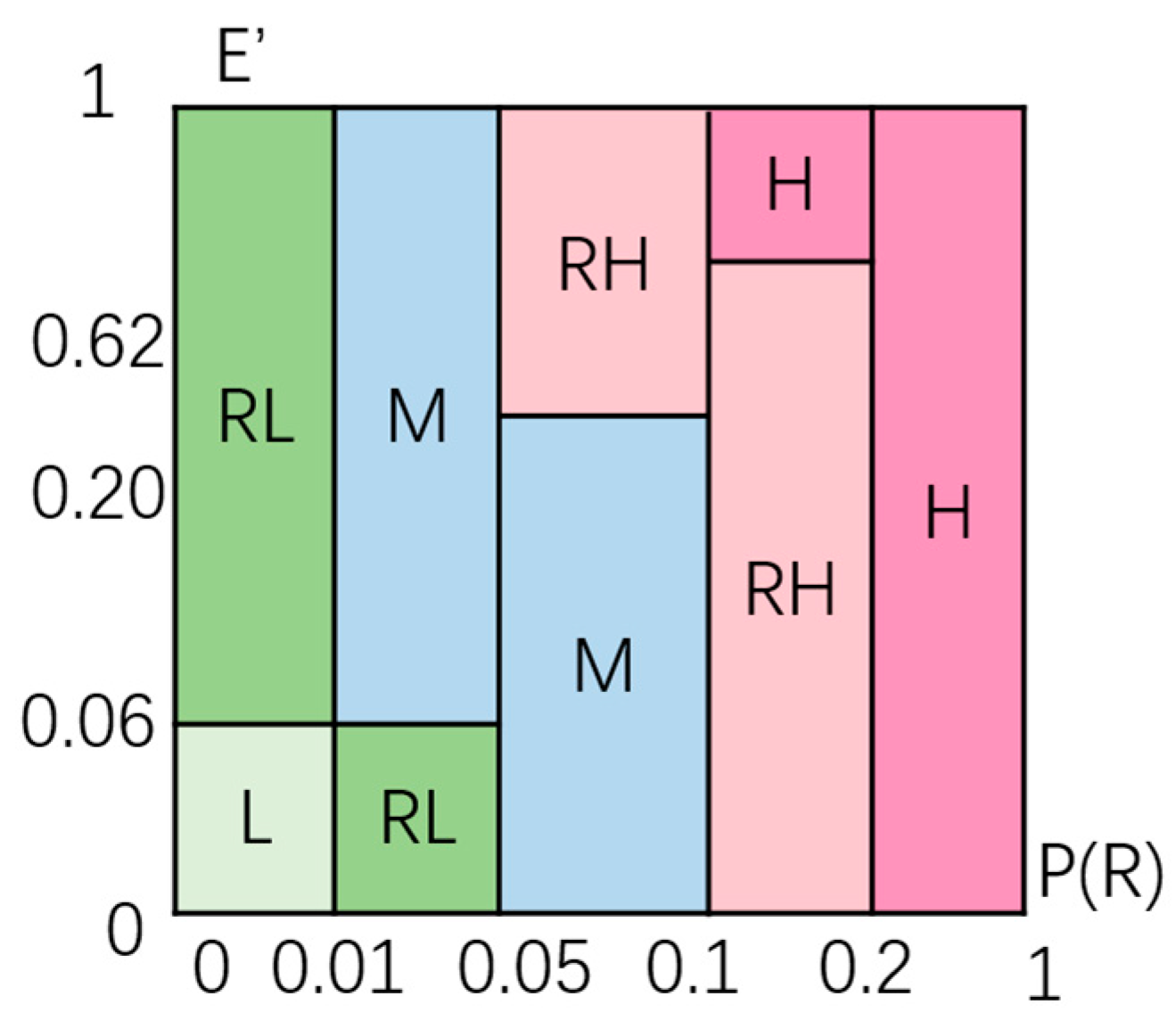
Through the above process, two values are obtained: the pipeline damage risk probability P(R) and the pipeline failure consequence E. The pipeline risk level is classified into five categories: high, relatively high, medium, relatively low, and low. The determination of the risk level is based primarily on the risk probability P(R), supplemented by the normalized failure consequence E′. For cases with relatively low consequence losses, the risk level is determined solely according to the probability classification; for cases with relatively high consequence losses, the risk level should be raised appropriately above that indicated by the probability classification. In this study, fuzzy logic relations [38] are applied, and the threshold values for risk-level classification specified in the Technical Specification for Geological Hazard Risk Management of Oil and Gas Pipelines (SY/T 6828-2024) [36] are referenced to establish a fuzzy-logic relationship diagram for determining the risk level, as shown in Figure 3.

5. Case Application and Analysis

The Phase I natural gas pipeline network of Jiangxi Natural Gas Company ([Nan Chang], China) has a total length of approximately 1020 km and forms a ring network around Poyang Lake through five main trunk lines, supplying gas to eight surrounding cities and several counties. The pipeline traverses areas with highly variable and complex topographic and geomorphological conditions. Jiangxi Province is located in a subtropical humid monsoon climate zone, characterized by mild temperatures and abundant rainfall. Influenced by typhoons, the region has an average annual precipitation of 1638 mm, with considerable spatial and temporal variability and pronounced interannual fluctuations. As a result, heavy rainfall and flash-flood events occur frequently.

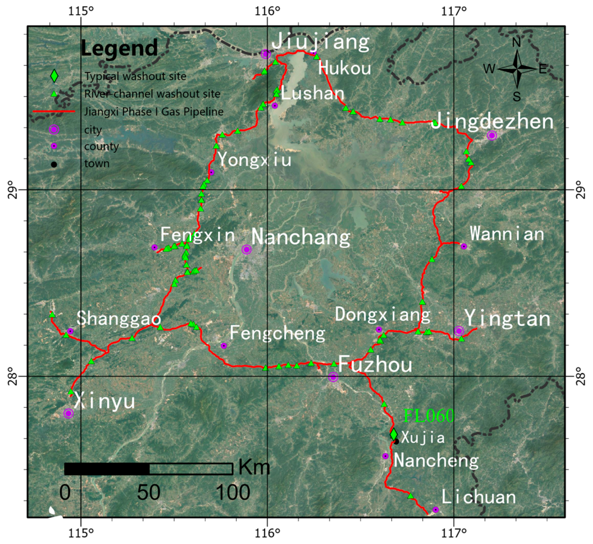
The Jiangxi natural gas pipeline network has been in operation for a relatively short period of time, and as of 2018, several branch lines were still under construction; thus, the system has not yet experienced major storm-flood events. According to recent geological disaster investigation reports, the spatial distribution of river-channel washout disasters is shown in Figure 4, with a total of 69 recorded washout sites. The distribution is spatially uneven: the number of sites is relatively high and densely concentrated in mountainous, hilly, and piedmont areas, whereas fewer sites occur in the plains and are more sparsely distributed. The risk levels are mainly medium and relatively low, with only a small number of relatively high-risk sites. In terms of failure modes, lateral erosion occurs slightly more frequently than vertical incision, though the numbers are relatively close.

In this study, 19 medium and small river-gully sites along the Phase I pipeline of Jiangxi Natural Gas Company—selected based on their potential hazards and early-warning significance, and constructed using open-cut trenching—are chosen as demonstration sites for the early-warning evaluation.

Using geographic information system (GIS) software, specifically ArcGIS Pro 3.5.2 (Esri, Redlands, CA, USA), the river centerlines and contour lines were determined based on high-resolution satellite remote-sensing images—such as QuickBird and WorldView—with spatial resolutions of 0.3–0.5 m, together with 1:50,000 vector topographic maps measured by the Jiangxi Surveying and Mapping Bureau. From these data, watershed and channel parameters such as main-channel length, drainage area, and weighted channel slope were extracted. In this study, the N-year return-period rainfall estimated by probabilistic methods is used to conduct the risk assessment of river-channel washout sites.

5.1. Calculation of Storm-Flood Discharge and River-Channel Scour Depth

Extreme rainfall and design flood estimation are closely related to hydrological frequency analysis [10,12,13]. In the statistical analysis of extreme hydrological events, extreme value theory, especially the Fisher–Tippett–Gnedenko theorem, provides an important theoretical basis for the limiting distribution of annual maximum series [13,14]. In engineering hydrological practice, probability distribution models such as the Gumbel distribution, generalized extreme value distribution, Pearson Type III distribution, and Log-Pearson Type III distribution are commonly used to estimate design rainfall or flood discharge under different return periods [11,12,13]. In this study, the Pearson Type III distribution was adopted based on regional hydrological practice and available rainfall statistics.

The areal rainfall corresponding to a design frequency of a% (i.e., a rainfall event with a return period of 1/a% years) is derived using probabilistic methods based on the Pearson Type III (P-III) probability distribution. The calculation formula is as follows:

$$P_{(a\%)} ={ P}_{\left(\mathit{annual} \mathit{max}\right)}·C_v·K_p\left(a\%\right)$$

(18)

In the equation, a% is the design frequency, corresponding to a return period of N = 1/a% years; P_{(annual max)} is the mean value of the annual maximum point rainfall, which can be obtained from regional meteorological data; C_v is the coefficient of variation of the annual maximum rainfall, which also depends on the statistical duration and can be determined from regional meteorological data; and K_p (a%) is the Pearson Type III probability-distribution value corresponding to the design frequency a%, calculated using the skewness coefficient C_s = 3.5C_v (where C_v is the coefficient of variation defined above), that is:

$$K_p\left(a\%\right) = 1 +{ C}_{\mathit{vt}}·\{{\displaystyle \frac{3.5·C_v}{2}}·f(1 - a\%,1,{\displaystyle \frac{2}{3.5·C_v}})-{\displaystyle \frac{2}{3.5·C_v}}\}$$

(19)

where f (x, β, α) is the probability density function of the gamma distribution. When β = 1, it becomes:

$$f\left(x,1,\alpha \right) = {\displaystyle \frac{x^{\alpha -1}}{{\int }_0^{+\infty }{g}^{\alpha -1}·e^{-g}\mathit{dg}}}·e^{-x}$$

(20)

${\int }_0^{+\infty }{g}^{\alpha -1}·e^{-g}\mathit{dg}$ is the Gamma function Γ(α), where g is the generalized integration variable.

Based on rainfall data statistics from the Jiangxi Hydrology Bureau, the mean values of the annual maximum point rainfall and the coefficients of variation of the annual maximum rainfall for rainfall durations of 1, 3, 6, and 24 h were obtained. According to the characteristics of the rainstorms, the areal design rainfall for durations of 1, 3, 6, and 24 h with design frequencies of 2% (50-year return period) and 1% (100-year return period) was calculated. On this basis, the areal rainfall for each time interval was determined. Finally, following the calculation procedures described above, rainfall–runoff generation, flow convergence, and the peak discharge together with the corresponding flow depth and velocity were computed for each of the 19 river-channel washout sites, and the scour depth of the river channels was ultimately obtained.

5.2. Risk Assessment Results and Discussion

The required information for each evaluation point of pipeline river-channel washout disasters was obtained from geological-disaster field investigations, hydrological data, and geological data. The risk early-warning calculations were then carried out following the methodological framework presented in this study. The computed risk probability P(R) and the corresponding risk levels under the 50-year and 100-year return-period storm-flood scenarios are presented in

Table 3. Output results of meteorological risk early-warning points for the Phase I Jiangxi Pipeline Network.

No.	Light to Moderate Rain		50-Year Return-Period Rainstorm		100-Year Return-Period Rainstorm
	P(R)	Risk Level	P(R)	Risk Level	P(R)	Risk Level
1	0.0048	RL	0.0215	M	0.0216	M
2	0.0020	RL	0.0081	RL	0.0087	RL
3	0.0078	RL	0.0078	RL	0.0078	RL
4	0.0042	RL	0.0042	RL	0.0042	RL
5	0.0016	RL	0.0016	RL	0.0016	RL
6	0.0280	M	0.0280	M	0.0280	M
7	0.0015	RL	0.0015	RL	0.0015	RL
8	0.0050	RL	0.0216	M	0.0232	M
9	0.0017	RL	0.0017	RL	0.0021	RL
10	0.0098	RL	0.0114	M	0.0175	M
11	0.0110	M	0.0110	M	0.0110	M
12	0.0026	RL	0.0026	RL	0.0026	RL
13	0.0196	M	0.0196	M	0.0196	M
14	0.0019	RL	0.0060	RL	0.0065	RL
15	0.0043	RL	0.0043	RL	0.0043	RL
16	0.0017	RL	0.0017	RL	0.0017	RL
17	0.0017	RL	0.0020	RL	0.0027	RL
18	0.0019	RL	0.0019	RL	0.0019	RL
19	0.0997	M	0.1474	RH	0.1488	RH

.

In the table, RL, M, and RH denote relatively low, medium, and relatively high risk, respectively. As shown in Table 3, the risk probabilities and risk levels of the 19 evaluation sites vary under different rainfall scenarios. Overall, under light-to-moderate rainfall conditions, the sites are mainly classified as relatively low risk and medium risk, with no relatively high-risk sites identified. Under the 50-year and 100-year return-period rainstorm scenarios, the risk probabilities of some sites increase, and the risk-level distribution changes from 15 relatively low-risk sites and 4 medium-risk sites under light-to-moderate rainfall conditions to 12 relatively low-risk sites, 6 medium-risk sites, and 1 relatively high-risk site. The responses of different sites to increasing rainfall intensity vary considerably. Site No. 19 has the highest risk probability and changes from medium risk to relatively high risk under stronger rainfall scenarios, while Sites No. 1, No. 8, and No. 10 also change from relatively low risk to medium risk. These results indicate that the proposed method can reflect the variation characteristics of river-channel washout risk under different rainfall scenarios and provide a basis for subsequent risk-level analysis and identification of key sites.

6. Conclusions and Recommendations

This study developed a quantitative risk assessment method for river-channel washout hazards affecting long-distance oil and gas pipelines by considering storm-flood-induced scour effects. The proposed method was applied to 19 river- and gully-crossing sites along the Phase I Jiangxi Natural Gas Pipeline Network. The main conclusions are as follows:

(1)

A risk assessment framework for river-channel washout hazards was established by coupling storm-flood rainfall–runoff calculation, peak discharge estimation, hydraulic parameter back-calculation, river-channel scour-depth calculation, pipeline vulnerability assessment, and failure consequence evaluation. The main innovation of this framework lies in converting storm-flood-induced river-channel scour effects into pipeline risk probability and risk level, thereby linking hydrological–hydraulic processes with pipeline engineering risk assessment.

(2)

The calculation results for the 19 evaluation sites along the Phase I Jiangxi Natural Gas Pipeline Network show that, under light-to-moderate rainfall conditions, the risk probability P(R) ranges from 0.0015 to 0.0997, with 15 sites classified as relatively low risk and 4 sites as medium risk. Under the 50-year return-period rainstorm scenario, P(R) ranges from 0.0015 to 0.1474, with 12 sites classified as relatively low risk, 6 sites as medium risk, and 1 site as relatively high risk. Under the 100-year return-period rainstorm scenario, P(R) ranges from 0.0015 to 0.1488, and the risk-level distribution remains 12 relatively low-risk sites, 6 medium-risk sites, and 1 relatively high-risk site.

(3)

The response of different evaluation sites to increasing rainfall intensity varies. Site No. 19 has the highest risk probability, increasing from 0.0997 under light-to-moderate rainfall conditions to 0.1474 and 0.1488 under the 50-year and 100-year return-period rainstorm scenarios, respectively, with its risk level increasing from medium risk to relatively high risk. Sites No. 1, No. 8, and No. 10 also change from relatively low risk to medium risk under stronger rainfall scenarios, indicating that these sites are relatively sensitive to storm-flood-induced scour.

(4)

The risk of river-channel washout is not controlled solely by rainfall intensity or scour depth, but is jointly influenced by factors such as pipeline burial depth, installation mode, affected pipeline length, protection works, direct pipeline protection measures, and failure consequences. At some evaluation sites, although the remaining soil cover thickness is insufficient under strong rainfall conditions, the final risk level does not increase significantly because the bed-protection and bank-protection measures are relatively effective. This indicates that both storm-flood-induced scour processes and pipeline engineering protection conditions should be considered in the risk assessment of river-channel washout hazards affecting pipelines.

(5)

The proposed method can be used for preliminary risk screening, flood-season risk classification, and inspection-priority determination for river- and gully-crossing sections of long-distance oil and gas pipelines. However, in engineering applications, the model parameters and risk-level classification results should be continuously calibrated using measured rainfall, water level, flow velocity, riverbed scour depth, pipeline burial depth, and the condition of protection works.

7. Discussion and Outlook

In recent years, risk assessment studies of pipeline geological hazards have gradually evolved from knowledge-driven methods, such as expert experience, analytic hierarchy process, and fuzzy comprehensive evaluation, to data-driven methods, including the information value model, neural networks, machine learning, multisource spatial data fusion, and interferometric synthetic aperture radar (InSAR)-based identification. These methods can effectively support regional-scale geological hazard susceptibility zoning and hazard-site ranking. However, most of them use static or semi-static factors, such as geomorphology, lithology, slope, land use, rainfall statistics, and historical hazard distribution, as the main inputs, and they insufficiently reflect the physical processes induced by a specific storm event. Compared with the above methods, this study does not simply propose a new statistical model or machine-learning algorithm. Instead, it incorporates the storm-flood-induced scour process into the pipeline risk assessment framework, so that the calculated river-channel scour results can be further converted into pipeline risk probability and risk level. This improves the physical interpretability and engineering applicability of river-channel washout risk assessment. Similar risk-decomposition ideas have also been proposed for other linear engineering projects under geohazard conditions, in which hazard probability, engineering vulnerability, and failure consequences are combined to support rapid and standardized risk screening [39].

From the calculation results, the risk probabilities of some sites increase with increasing rainfall intensity, but not all sites show significant changes. This is partly related to the structure of the proposed model. Rainfall intensity mainly affects the river-channel scour-intensity indicator through peak discharge, flow velocity, flow depth, and scour depth, whereas indicators such as pipeline installation mode, affected pipeline length, protection condition, and failure consequence generally remain unchanged under different rainfall scenarios. Therefore, the final risk probability does not increase proportionally with rainfall intensity. This result is also related to the engineering conditions of the study area. Although some sites are subject to a certain degree of scour risk, relatively effective bed-protection or bank-protection measures have been implemented, which weakens the influence of increased rainfall intensity on the final risk level. Therefore, the limited variation in risk probability shown in Table 3 does not necessarily indicate model failure, but rather reflects the combined control of storm-flood-induced scour and pipeline engineering protection conditions on river-channel washout risk.

It should be noted that the multiplicative form used in the proposed risk model should be understood as a semi-quantitative engineering risk-index aggregation method, and it does not imply that all evaluation indicators are strictly independent in a statistical sense. The index values for protection effectiveness, pipeline vulnerability, and other factors are mainly determined based on technical specifications, field investigations, and engineering experience, rather than being calibrated using a large historical failure database. In addition, uncertainties exist in rainfall–runoff parameters, riverbed material particle size, channel roughness, and scour-calculation parameters. Considering the limited availability of continuous discharge, water-level, and flood-process observations for most investigated seasonal gullies, the uncertainty of empirical parameters was discussed qualitatively in this study. Future work should combine measured rainfall, water level, flow velocity, and post-flood scour-depth data to conduct quantitative sensitivity analysis of key empirical parameters and further calibrate the model. Therefore, before the proposed method is further incorporated into a pipeline integrity management system, rainfall–runoff calculation, scour-depth estimation, index assignment, and risk-level thresholds should be validated and revised using measured rainfall, water level, flow velocity, post-flood scour depth, pipeline burial-depth remeasurement, and long-term inspection data.

Future studies can incorporate real-time hydrometeorological monitoring, unmanned aerial vehicle (UAV) inspection, remote sensing imagery, underwater inspection, and other data into the existing framework to dynamically update the risk probability and risk level of river-channel washout hazards. This idea is also consistent with recent pipeline safety assessment frameworks that emphasize GIS-based integration of multisource monitoring data and dynamic risk-level updating for pipeline safety management [7]. With the accumulation of monitoring data and historical cases, model parameters and risk thresholds can be continuously optimized, thereby improving the applicability of the proposed method in dynamic flood-season early warning and pipeline management.