A Study on Three-Dimensional Resistivity Model Construction Based on Spherical Radial Basis Function Interpolation

Abstract

The spatial distribution of strata under nappe tectonic conditions is highly complex. Conventional approaches, such as dense borehole exploration or intensive in situ investigation, are often costly and difficult to implement for revealing detailed stratigraphic structures. To address this issue, this study focuses on the nappe tectonic setting of the main orebody in the Kambove mining area and proposes a spherical radial basis function interpolation method incorporating spatial anisotropy to construct a three-dimensional resistivity model, thereby providing a data foundation for subsequent intelligent stratigraphic identification. First, the discrete resistivity measurement points were processed through coordinate unification, elevation correction, and data quality inspection. Then, based on radial basis function interpolation theory, a spherical kernel function and anisotropic ellipsoidal constraints were introduced to achieve the three-dimensional continuous representation of discrete resistivity data. Finally, the interpolation performance of the proposed method was compared with that of linear RBF interpolation and inverse distance weighting with $P=2$ and $P=3$ using random holdout validation. The spherical RBF method yielded an ME of −12.2 Ω·m and the lowest RMSE of 299.0 Ω·m, corresponding to RMSE reductions of 13.6–22.0% relative to the comparison methods. These results indicate that the spherical RBF method provides better local interpolation performance within areas covered by existing measurements. The proposed method preserves the continuity and smoothness of the resistivity field and enhances its representation along the dominant geological structural direction, thereby providing a continuous three-dimensional resistivity basis for subsequent intelligent stratigraphic identification.

1. Introduction

Geophysical exploration provides an efficient and cost-effective means of characterizing stratigraphic distributions, as resistivity, a regionalized variable reflecting variations in the electrical properties of subsurface media, is jointly controlled by factors such as ore grade, water-bearing conditions, and fault–fracture development, thereby enabling different strata to be distinguished by their characteristic resistivity signatures [1,2,3,4]. In applications of the high-density electrical resistivity method, most existing studies are based primarily on two-dimensional inversion profiles, which makes it difficult to accurately characterize the continuous variation in geological bodies outside the survey lines and along the planar direction [5,6]. To address this issue, Hung et al. [7] developed a three-dimensional numerical model to simulate the effects of off-line pipelines, boundary undulations, and resistivity contrasts on two-dimensional electrical resistivity inversion profiles, demonstrating that two-dimensional resistivity interpretation in three-dimensional heterogeneous strata is susceptible to interference from off-line objects. Mishra et al. [8] proposed a quasi-three-dimensional modeling approach to overcome the time-consuming and labor-intensive nature of regular-grid resistivity surveys and their susceptibility to site obstacles, in which the azimuths of non-parallel two-dimensional resistivity inversion profiles were used to introduce y-coordinates for constructing a three-dimensional database, thereby enhancing the spatial visualization of conductive bodies. Jia et al. [9] addressed the limitations of high-density electrical resistivity data, which are commonly acquired along profiles and interpreted through two-dimensional inversion with poor consistency between adjacent survey lines, by employing an irregular “#”-shaped profile layout to supplement lateral information and constructing a resistivity-based geological model using three-dimensional visualization software, thereby achieving the three-dimensional representation of electrical properties in complex goaf subsidence areas. Therefore, transforming two-dimensional resistivity data into a continuous three-dimensional resistivity volume is essential for improving the intuitive representation of results and enhancing the reliability of engineering interpretation.

Spatial interpolation methods provide an effective approach for transforming discrete data into continuous three-dimensional representations, with commonly used techniques including kriging, inverse distance weighting, and radial basis function interpolation [10,11]. Liu et al. [12] coupled the K-nearest neighbor algorithm with kriging for complex three-dimensional geological modeling and improved the accuracy of three-dimensional stratigraphic modeling through virtual borehole densification and data standardization, indicating that relying solely on original sparse data in kriging-based modeling is often insufficient for refined modeling and that data densification and spatial prediction methods are required to enhance model representation. Liu et al. [13] applied inverse distance weighting to three-dimensional geological modeling and demonstrated that its computational accuracy is strongly affected by the search radius and weighting exponent; moreover, because these conventional parameters are commonly determined empirically, the applicability of standard inverse distance weighting is limited under conditions of strong spatial variability. In contrast, radial basis function interpolation constructs a continuous scalar field using kernel functions, thereby enabling an effective three-dimensional continuous representation of discrete attribute points, and is characterized by smooth modeling, a unified computational formulation, and suitability for modeling complex spatial attributes [14]. Zhang et al. [15] employed the radial basis function method to process multilayer stratigraphic interface points and attitude information, thereby establishing a continuous three-dimensional stratigraphic potential field that effectively represented the spatial variation in complex stratigraphic interfaces. Hillier et al. [16] used radial basis functions to perform three-dimensional modeling of discrete geological contact points and attitude constraints, producing continuous, smooth, and spatially reasonable geological interfaces.

These findings indicate that although kriging and inverse distance weighting can be used for discrete attribute interpolation, they are respectively limited by insufficient representation of spatial structures and sensitivity to spatial variability in complex geological settings, whereas radial basis function interpolation is more suitable for transforming discrete x-, y-, z-, and $\rho$-point data derived from multi-line resistivity inversion results into a continuous three-dimensional resistivity model, thereby enabling the continuous three-dimensional representation of resistivity.

Based on these considerations, this study adopts a spherical radial basis function interpolation method to construct a three-dimensional resistivity model from high-density electrical resistivity data of the main orebody in the Kambove mining area by continuously representing discrete resistivity measurement points in three-dimensional space, while spatial anisotropic constraints are incorporated into the interpolation process to enhance the model’s ability to characterize geological directional features, ensuring reasonable continuity along the dominant geological structural direction and preventing unnecessary overextension in other directions, thereby providing a continuous data foundation for subsequent research on intelligent stratigraphic identification models.

2. Research Background and Fundamental Data

2.1. Geological Background of the Main Orebody in the Kambove Mining Area

The Kambove main orebody is located on the Katanga Plateau in southeastern Democratic Republic of the Congo. The mining area lies within the Katanga fold–thrust belt and forms part of the Central African Lufilian Arc. Influenced by regional tectonic evolution, the area has undergone multiple stages of thrusting, compression, and tectonic superposition, resulting in complex contact relationships and spatial assemblages among different geological blocks. Consequently, the main orebody and its surrounding rocks exhibit pronounced spatial heterogeneity and directional characteristics [17,18,19,20].

The principal stratigraphic units developed in the mining area include the Kundelungu Group, Nguba Group, and Roan Group, among which the Roan Group represents an important regional ore-bearing horizon and is mainly composed of clastic rocks, argillaceous rocks, and carbonate rocks [21]. According to existing geological data from the mining area, the main orebody and its adjacent surrounding rocks can be further subdivided into several stratigraphic assemblage units, including KU, CMN, SD, RSC, RSF, RAT, and BR. These stratigraphic assemblages differ in mineral composition, structural integrity, pore–fracture development, water-bearing conditions, and degree of weathering, leading to spatial variations in resistivity properties. To intuitively characterize the spatial distribution of resistivity properties within the main orebody, this study constructs a three-dimensional resistivity model using high-density electrical resistivity data from the Kambove main orebody and the spherical radial basis function interpolation method.

2.2. Acquisition and Preprocessing of High-Density Electrical Resistivity Data

The fundamental data used in this study consist of high-density electrical resistivity survey data from the Kambove main orebody. These data are recorded using individual measurement points as the basic units and include information such as point ID, planar coordinates, elevation, resistivity value, and survey-line number. According to the topographic conditions of the mining area and the spatial distribution characteristics of the main orebody, the high-density electrical resistivity survey lines were mainly arranged along the benches of the open-pit mine. A total of 36 survey lines were deployed, each extending along the bench trend and collectively covering the key exploration area of the main orebody.

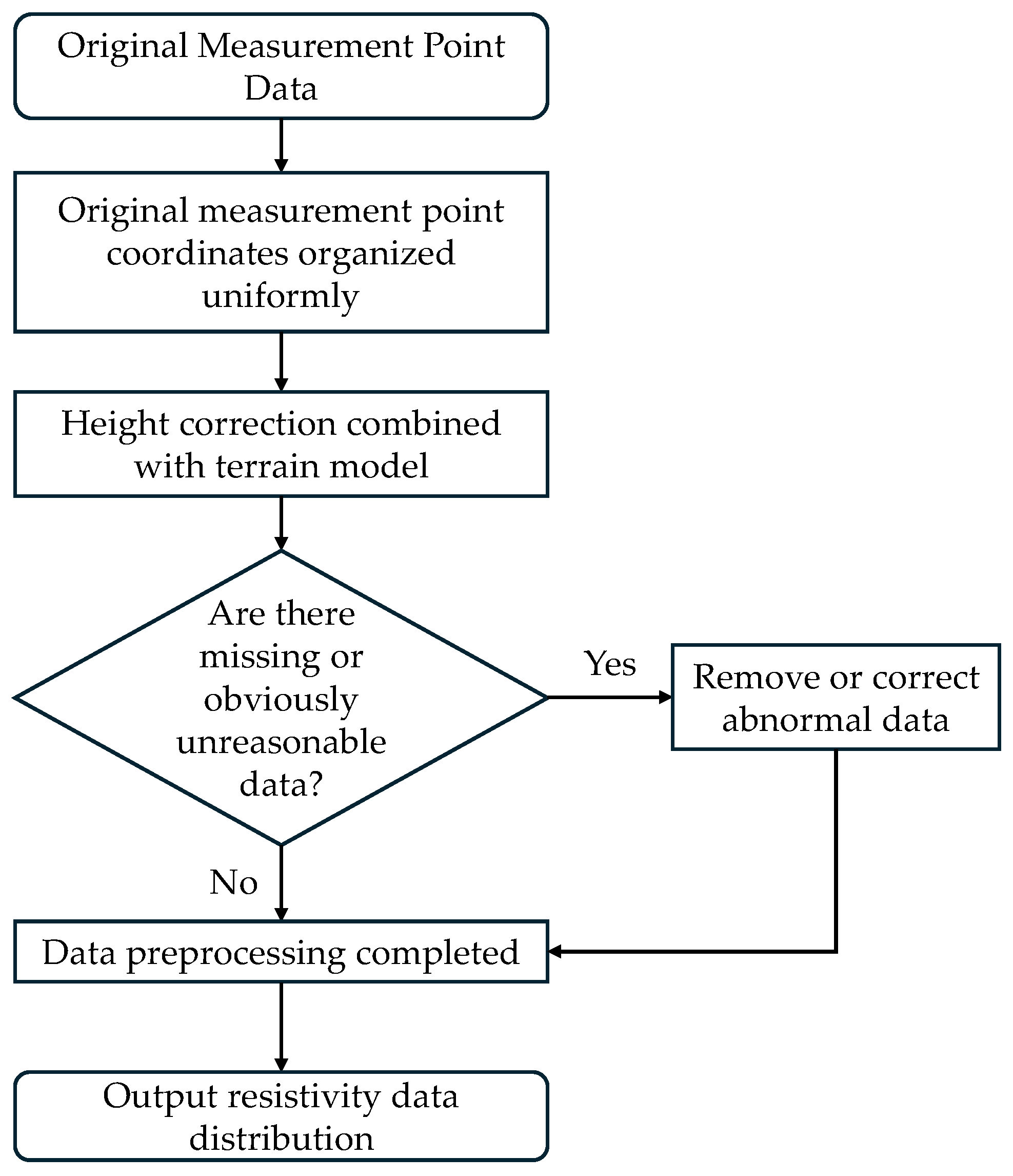
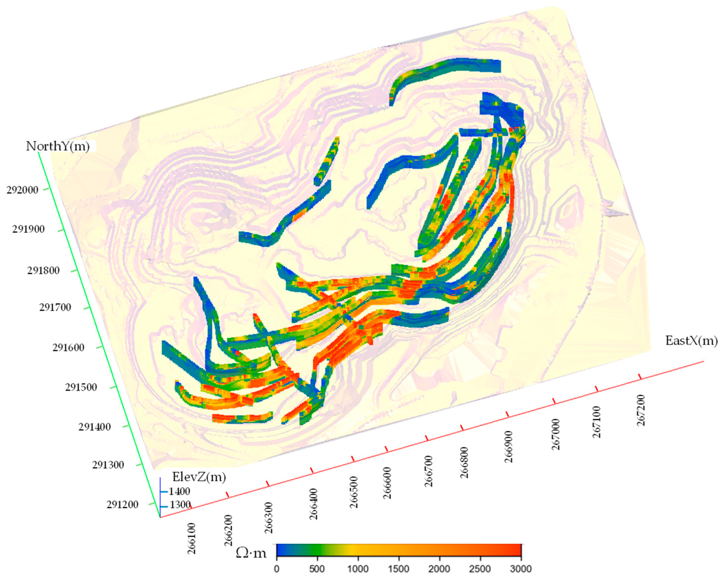
Prior to interpolation, the raw high-density electrical resistivity data were preprocessed, as shown in Figure 1. First, the coordinates of the original measurement points were uniformly organized to ensure that different survey lines and data batches were integrated within the same coordinate system. Second, the elevations of the measurement points were corrected based on the terrain model, allowing the resistivity data to accurately represent their actual positions in three-dimensional space. Subsequently, data completeness and consistency were checked, and missing or obviously unreasonable data were removed or corrected. The final spatial distribution of the resistivity data is shown in Figure 2.

3. Spherical Radial Basis Function Interpolation Method Considering Spatial Anisotropy

3.1. Overview of the Radial Basis Function Interpolation Method

To address the discrete distribution of high-density electrical resistivity data, the insufficient spatial continuity between survey lines, and the difficulty in three-dimensional representation of complex geological bodies, this study introduces radial basis function interpolation to construct a three-dimensional resistivity model. The radial basis function is an exact interpolation method that can be readily extended to high-dimensional spaces. This interpolation method originally emerged in the field of geosciences and has been used to describe the correlation characteristics of spatial interpolation [22]. Its basic principle can be expressed as follows:

$$s(x)=p(x)+{\displaystyle \sum _{i=1}^n{w}_i}\varphi (r_i)$$

(1)

where $s\left(x\right)$ denotes the attribute value, $\varphi$ is the radial basis kernel function, $r_i$ represents the Euclidean distance between the interpolation point and the known sampling point, $w_i$ is the interpolation weight coefficient, and $p\left(x\right)$ denotes a polynomial term.

3.2. Spherical Radial Basis Function Considering Spatial Anisotropy

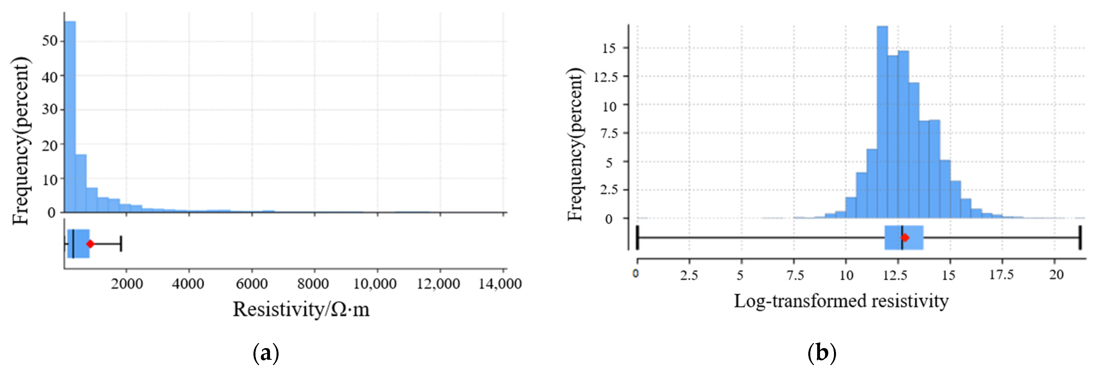
Considering that resistivity is a regionalized variable, a logarithmic transformation was first applied to the original observed resistivity values ${\rho }_i$ prior to modeling, in order to reduce the influence of the large magnitude range of discrete high-density electrical resistivity measurements on the stability of spatial interpolation (Figure 3) [23]. The logarithmic value of the observed target physical property, $z_i$, is defined as follows:

$${\widehat{z}}_i=\ln ({\rho }_i-1.5)+6.9$$

(2)

Geostatistics is based on regionalized variables and uses the semivariogram as a tool to describe spatial correlation [24]. The semivariogram, also referred to as the semivariance function, can characterize both the randomness and structural properties of regionalized variables, making it an effective tool for analyzing spatial variation patterns and spatial structures. Half of the variance of the difference between the values $Z\left(x_i\right)$ and $Z\left(x_i+h\right)$ of the regionalized variable $Z\left(x\right)$ at locations $x_i$ and $x_i+h$, respectively, is defined as the semivariogram of $Z\left(x\right)$ [25], namely:

$$j(h)={\displaystyle \frac{1}{2N(h)}}{\displaystyle \sum _{i=1}^{N(h)}{\left[Z(x_i)-Z(x_i+h)\right]}^2}$$

(3)

where $j\left(h\right)$ denotes the semivariogram; $Z\left(x\right)$ is the regionalized random variable; $h$ represents the separation distance between two sampling points; and $N\left(h\right)$ is the number of observation point pairs separated by the lag distance $h$. $Z\left(x_i\right)$ and $Z\left(x_i+h\right)$ are the measured values of the regionalized variable $Z\left(x\right)$ at locations $x_i$ and $x_i+h$, respectively.

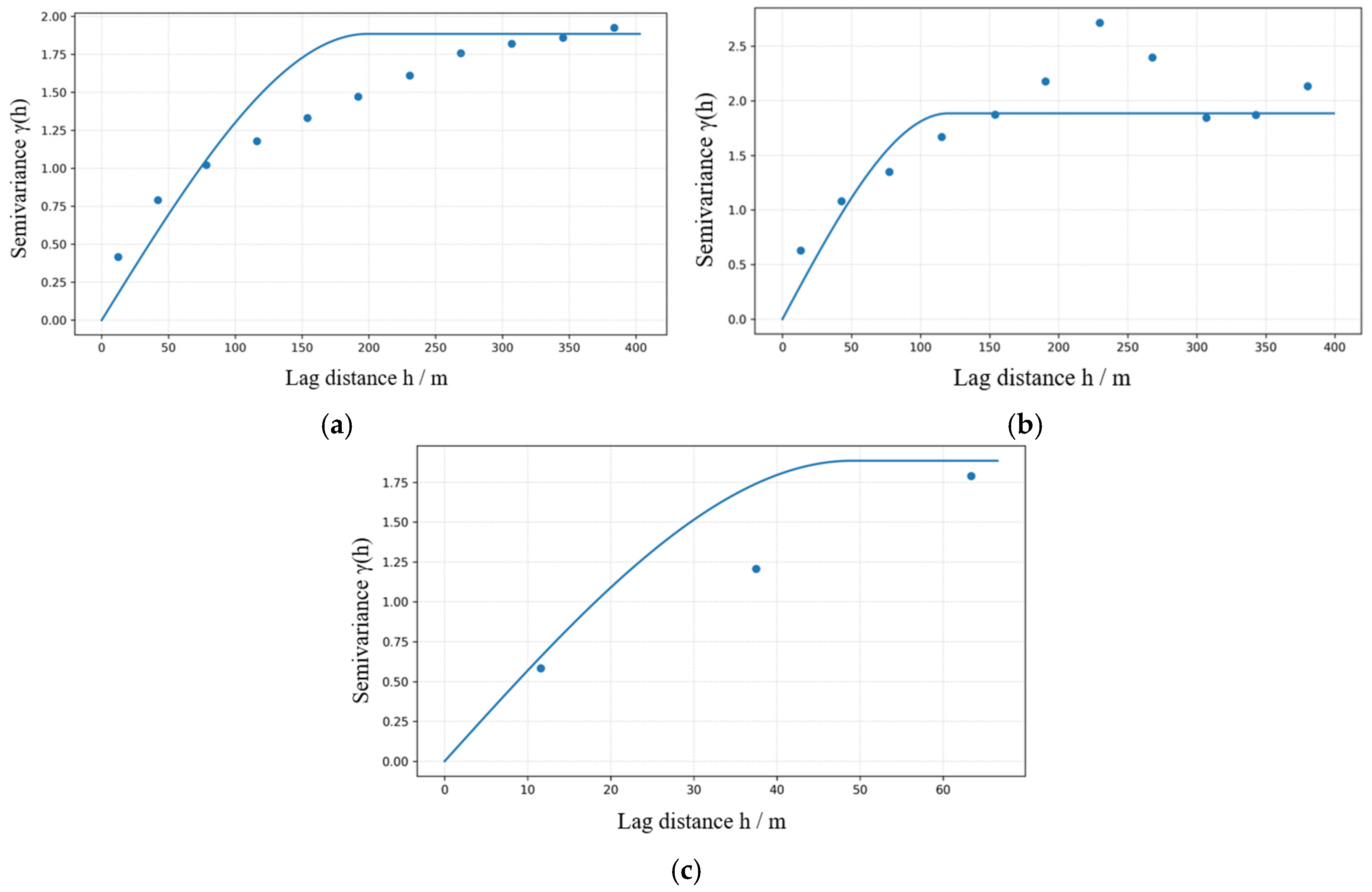
After applying logarithmic transformation to the original resistivity data, semivariogram analyses were conducted along the major axis, semi-major axis and minor axis directions, respectively, and the results were fitted using a spherical model, as shown in Figure 4.

As shown in Figure 4, the directional semivariograms can be fitted using a spherical model, with a total sill of 1.91 and directional ranges of 200, 120, and 49 m along the major, intermediate, and minor continuity directions, respectively, indicating pronounced spatial anisotropy. Taking the major axis range as the reference, the normalized ellipsoidal axis ratios are:

$${\eta }_1:{\eta }_2:{\eta }_3=1:\frac{120}{200}:\frac{49}{200}=1:0.6:0.245$$

The total sill characterizes the overall spatial variation amplitude of the log-transformed resistivity, whereas the directional ranges determine the shape and scaling of the anisotropy ellipsoid. Therefore, only the directional ranges and orientation parameters are used to construct the anisotropic distance transformation matrix.

A global Cartesian coordinate system was defined with the $X$ axis pointing east, the $Y$ axis pointing north, and the $Z$ axis pointing upward. For an interpolation point $x$ and the $i$-th observation point $x_i$, their coordinate difference is:

$$\Delta x_i=x-x_i=\left[\begin{array}{c}X-X_i\\ Y-Y_i\\ Z-Z_i\end{array}\right]$$

(4)

The spatial orientation of the anisotropy ellipsoid is described by the dip azimuth $\alpha$, dip angle $\beta$, and pitch angle $\psi$. The dip azimuth and dip angle jointly define the plane containing the major and intermediate axes of the ellipsoid, whereas the pitch angle defines the orientation of the major axis within this plane.

The unit vectors along the strike direction, down-dip direction, and normal direction of the major–semi-major axis plane are defined as:

$$s=\left[\begin{array}{c}\cos \alpha \\ -\sin \alpha \\ 0\end{array}\right],\hspace{1em}d=\left[\begin{array}{c}\sin \alpha \cos \beta \\ \cos \alpha \cos \beta \\ -\sin \beta \end{array}\right],\hspace{1em}n=\left[\begin{array}{c}\sin \alpha \sin \beta \\ \cos \alpha \sin \beta \\ \cos \beta \end{array}\right]$$

(5)

The unit vectors along the major, intermediate, and minor axes of the anisotropy ellipsoid are then expressed as

$${\mathbf{e}}_1=\cos \psi \mathbf{s}+\sin \psi \mathbf{d},{\mathbf{e}}_2=-\sin \psi \mathbf{s}+\cos \psi \mathbf{d},{\mathbf{e}}_3=\mathbf{n}.$$

(6)

Here, $e_1$, $e_2$ and $e_3$ represent the directions of the major, intermediate, and minor axes, respectively. When $\psi =0^{\circ }$, the major axis is parallel to the strike direction. As $\psi$ increases, the major axis rotates within the major–semi-major axis plane toward the down-dip direction.

The three unit vectors form the orthogonal rotation matrix

$$R=\left[\begin{array}{ccc}{e}_1& e_2& e_3\end{array}\right],\hspace{1em}{R}^{T}R=I.$$

(7)

The normalized directional ranges are:

$${\eta }_1=1,\hspace{1em}{\eta }_2=0.600,\hspace{1em}{\eta }_3=0.245,$$

(8)

and the corresponding directional scaling matrix is

$$S=\mathrm{diag}\left(1,{\displaystyle \frac{1}{{\eta }_2}},{\displaystyle \frac{1}{{\eta }_3}}\right)=\mathrm{diag}\left(1,{\displaystyle \frac{1}{0.600}},{\displaystyle \frac{1}{0.245}}\right)=\mathrm{diag}\left(1,1.6667,4.0816\right).$$

(9)

The anisotropic coordinate transformation matrix $V$ and the corresponding metric tensor $M$ are defined as

$$V=S{R}^T,\hspace{1em}M=V^{T}V=R{S}^2{R}^T.$$

(10)

Accordingly, the anisotropic distance between the interpolation point and the $i$-th observation point is calculated as

$$r_i^{(a)}=\Vert V\Delta x_i{\Vert }_2=\sqrt{\Delta x_i^{T}M\Delta x_i}$$

(11)

For the Kambove main orebody, the ellipsoid orientation parameters determined from the dominant structural and fracture-zone trends were:

$$\beta =0°,\hspace{1em}\alpha =57°,\hspace{1em}\psi =90°$$

Under these orientation parameters, the major axis is horizontal with an azimuth of $57°$, the semi-major axis is horizontal and perpendicular to the major axis, and the minor axis is vertical. The resulting rotation matrix is:

$$R=\left[\begin{array}{ccc}0.8387& -0.5446& 0\\ 0.5446& 0.8387& 0\\ 0& 0& 1\end{array}\right]$$

(12)

The anisotropic transformation matrix is therefore:

$$V=\left[\begin{array}{ccc}0.8387& 0.5446& 0\\ -0.9077& 1.3978& 0\\ 0& 0& 4.0816\end{array}\right]$$

(13)

and the corresponding anisotropic metric tensor is

$$M=\left[\begin{array}{ccc}1.5273& -0.8120& 0\\ -0.8120& 2.2504& 0\\ 0& 0& 16.6597\end{array}\right]$$

(14)

Alternatively, the coordinate difference can first be projected onto the local coordinate system of the ellipsoid:

$$q_i=R^T\Delta x_i=\left[\begin{array}{c}{q}_{1i}\\ q_{2i}\\ q_{3i}\end{array}\right]=\left[\begin{array}{c}0.8387\Delta X_i+0.5446\Delta Y_i\\ -0.5446\Delta X_i+0.8387\Delta Y_i\\ \Delta Z_i\end{array}\right]$$

(15)

The anisotropic distance can then be equivalently written as

$$r_i^{(a)}=\sqrt{q_{1i}^2+{\left({\displaystyle \frac{q_{2i}}{0.600}}\right)}^2+{\left({\displaystyle \frac{q_{3i}}{0.245}}\right)}^2}$$

(16)

This transformation expands the distances along the intermediate and minor axes by factors of $1/0.600$ and $1/0.245$, respectively, thereby converting the original anisotropic ellipsoid into an equivalent spherical coordinate system. When the support-range parameter of the spherical kernel is set to $a=200 \mathrm{m}$, the corresponding effective ranges along the major, intermediate, and minor axes are

$$a{\eta }_1=200 \mathrm{m},\hspace{1em}a{\eta }_2=120 \mathrm{m},\hspace{1em}a{\eta }_3=49 \mathrm{m}$$

which are consistent with the directional semivariogram fitting results.

In radial basis function interpolation, the selection of the kernel function $\varphi \left(r\right)$ directly affects the smoothness of the interpolation results, the ability to represent local variations, and computational stability. Different kernel functions respond differently to the spatial distance r, and are therefore suitable for different types of spatial attribute modeling problems. Common radial basis kernel functions [26] are listed in

Table 1. Common radial basis kernel functions.

Serial Number	Function Name	Radial Basis Kernel Functions
1	Gaussian Kernel Function	$\varphi (r)=e^{-{(cr)}^2}$
2	Multiple Quadratic Functions	$\varphi (r)=\sqrt{r^2+c^2}$
3	Thin-Plate Spline Kernel Function	$\varphi (r)=r^2\log r$
4	Spherical Compactly Supported Function	$\varphi (r)=\left\{\begin{array}{ll}1-{\displaystyle \frac{3r}{2a}}+{\displaystyle \frac{r^3}{2a^3}},\hfill & 0\le r\le a\hfill \\ 0,\hfill & r>a\hfill \end{array}\right.$
5	Linear Radial Basis Function Kernel	$\begin{array}{l}\varphi (r)=r\end{array}$

Note: r denotes the distance between two points; c is the shape parameter; and a is the range parameter.

.

In this study, a spherical radial basis kernel function with compact support was selected as the interpolation kernel to enhance the model’s ability to represent the spatially continuous variation in resistivity properties. where $r$ is replaced by the anisotropic distance $r_i^{\left(a\right)}$, and $a$ is the support-range parameter. This function can effectively fit the smooth and continuous spatial variation trend of geological attributes while maintaining the relative stability of attribute distributions within local regions.

Considering the geological structural characteristics of the Kambove mining area and the density of the high-density electrical resistivity survey grid, the parameters of the mathematical model were rigorously defined as follows (

Table 2. Radial basis function interpolation parameters.

Range Parameter	Regularization Parameter	Global Trend Term	Anisotropic Direction Parameters	Anisotropic Ellipsoid Axis Ratios
200	${10}^{-5}$	zeroth-order constant trend term	Dip = 0°	major axis = 1
			Dip Azimuth = 57°	semi-major axis = 0.6
			Pitch = 90°	minor axis = 0.245

):

(1)

Range parameter: The range parameter was set to $a=200$ m. Given that the range along the major axis direction is 200 m, setting $a=200$ m preserves the spatial correlation along the dominant continuity direction.

(2)

Regularization parameter: To reduce the influence of measurement noise in field resistivity data, a weak Tikhonov regularization term was introduced into the radial basis function interpolation equation, with the regularization parameter set to $\lambda ={10}^{-5}$. Faiyaz et al. [27] adopted a Tikhonov regularization parameter of the same magnitude in an RBF-network-based electrical impedance tomography inverse problem and demonstrated that regularization can mitigate overfitting and improve reconstruction stability for unseen data. Accordingly, $\lambda ={10}^{-5}$ was adopted in this study as a weak non-zero regularization parameter, allowing moderate smoothing of measurement noise and local anomalies while substantially preserving the constraints imposed by the measured log-transformed resistivity values.

(3)

Global trend term: To control the convergence behavior of the field function in boundary and deep extrapolation regions, a zeroth-order constant trend term was introduced as the polynomial form of $p\left(x\right)$. This setting guides the field function to converge smoothly toward the regional background mean of the physical property in deep marginal areas without control points, thereby effectively preventing mathematical divergence and abnormal distortion at the model boundaries.

3.3. Discrete Solution of the Scalar Field Array and Coefficient Matrix Solving

After establishing the anisotropic spherical kernel function model, the core mathematical task of radial basis function interpolation is to solve the interpolation weight coefficient vector $W$ and the trend-term coefficient vector $A$ corresponding to each sampling point. Based on the function-value constraint at the sampling points, $s\left(x_i\right)$ = $z_i$, and the polynomial orthogonality constraint, the following system of linear equations can be constructed [28]:

$$\left[\begin{array}{cc}K+\lambda I& P\\ P^T& 0\end{array}\right]\left[\begin{array}{c}W\\ A\end{array}\right]=\left[\begin{array}{c}Z\\ 0\end{array}\right]$$

(17)

where $K$ is an $n\times n$ symmetric radial basis function matrix whose arbitrary element is defined as $K_{ij}=\varphi \left(r_{ij}^{’}\right)$, characterizing the spatial correlation induced by geometric anisotropy between each pair of known observation points. I denotes the $n\times n$ identity matrix, and $\lambda I$ is a diagonal Tikhonov regularization term introduced to improve the numerical stability of the system and balance fidelity to the observations against the smoothness of the interpolated field. In this study, the regularization parameter was set to $\lambda ={10}^{-5}$. This weak non-zero regularization permits slight deviations from exact interpolation, thereby reducing sensitivity to measurement noise and local anomalies while largely preserving the constraints imposed by the observed data. $P$ is an $n\times m$ low-order global trend polynomial matrix. Under the zeroth-order constant trend term adopted in this study, $m=1$, and $P$ is represented by an $n\times 1$ column vector of ones. $W$ is the $n\times 1$ vector of interpolation weight coefficients to be determined, expressed as $W={[w_1,w_2,\dots ,w_n]}^T$; $A$ is the $m\times 1$ vector of unknown polynomial coefficients associated with the global trend term; and $Z$ is the $n\times 1$ vector of known target values of the observed scalar field, namely, the log-transformed discrete measured resistivity data: $Z={[z_1,z_2,\dots ,z_n]}^T$.

4. Three-Dimensional Resistivity Field Modeling Results

4.1. Three-Dimensional Resistivity Model

An adaptive-resolution meshing technique was employed to discretize the study area into three-dimensional regular voxels with a base resolution of 2.5 m. Subsequently, the established continuous radial basis function scalar field was evaluated at the center of each voxel to obtain the predicted log-transformed resistivity values. These values were then converted back to the original resistivity scale using the inverse transformation:

$${\widehat{\rho }}_i=e^{\left({\widehat{z}}_i-6.9\right)}+1.5$$

(18)

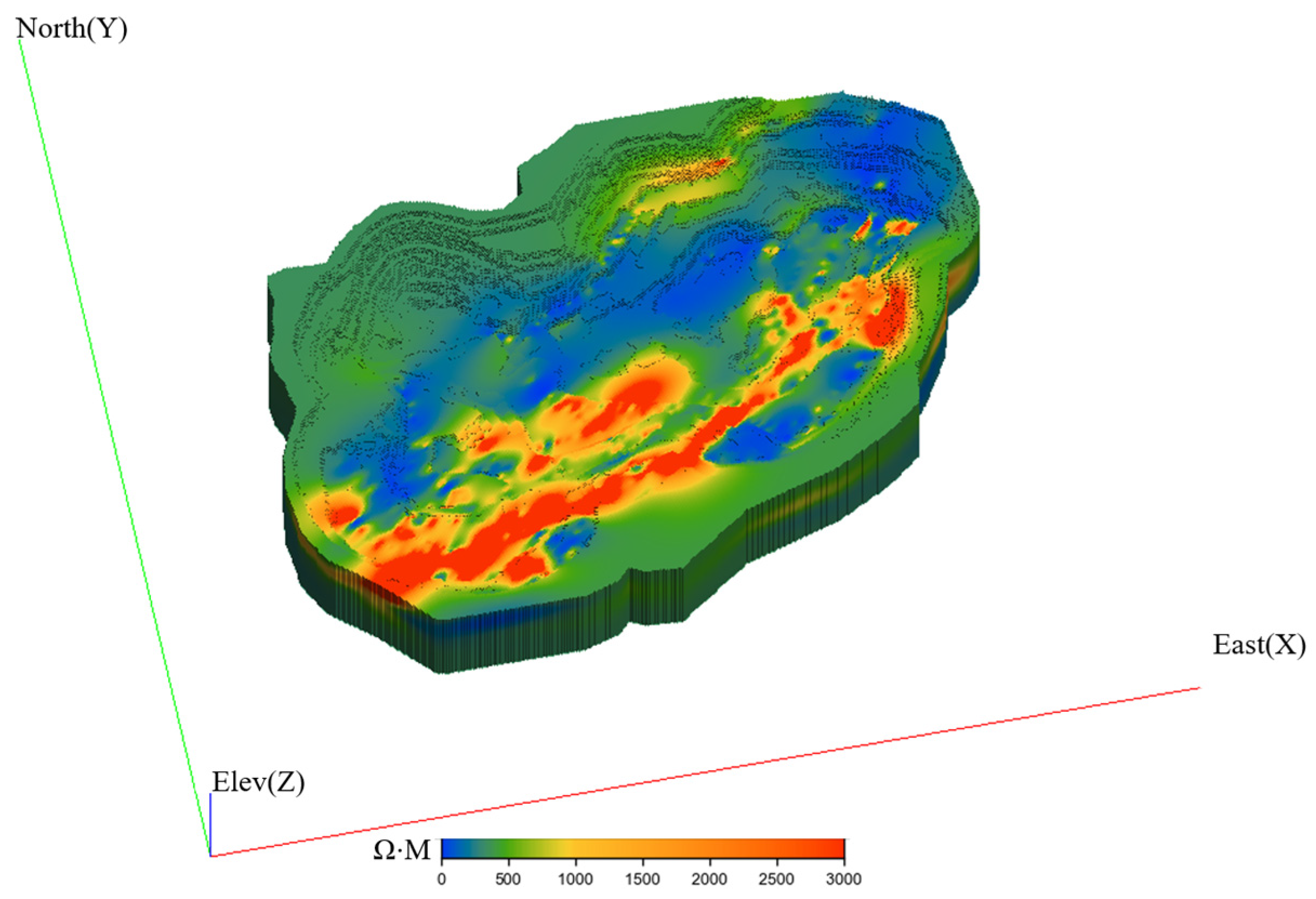
where ${\widehat{z}}_i$ denotes the predicted log-transformed resistivity value and ${\widehat{\rho }}_i$ denotes the corresponding resistivity value on the original scale. The resulting three-dimensional resistivity model is shown in Figure 5.

The three-dimensional resistivity model reveals pronounced spatial heterogeneity and continuous variations in resistivity across the mining area. Overall, high-resistivity zones are predominantly concentrated from the south-central to southeastern parts of the model and locally exhibit continuous patchy or belt-like distributions. Low-resistivity zones are mainly distributed in the northern, northeastern, and some central areas, showing a certain degree of spatial continuity. Moderate-resistivity zones are more widely distributed and generally occur between the high- and low-resistivity zones, forming relatively smooth transitional belts. These modeling results indicate that resistivity within the mining area varies significantly in both the horizontal and vertical directions.

4.2. Comparative Evaluation and Random Holdout Validation of the Resistivity Model

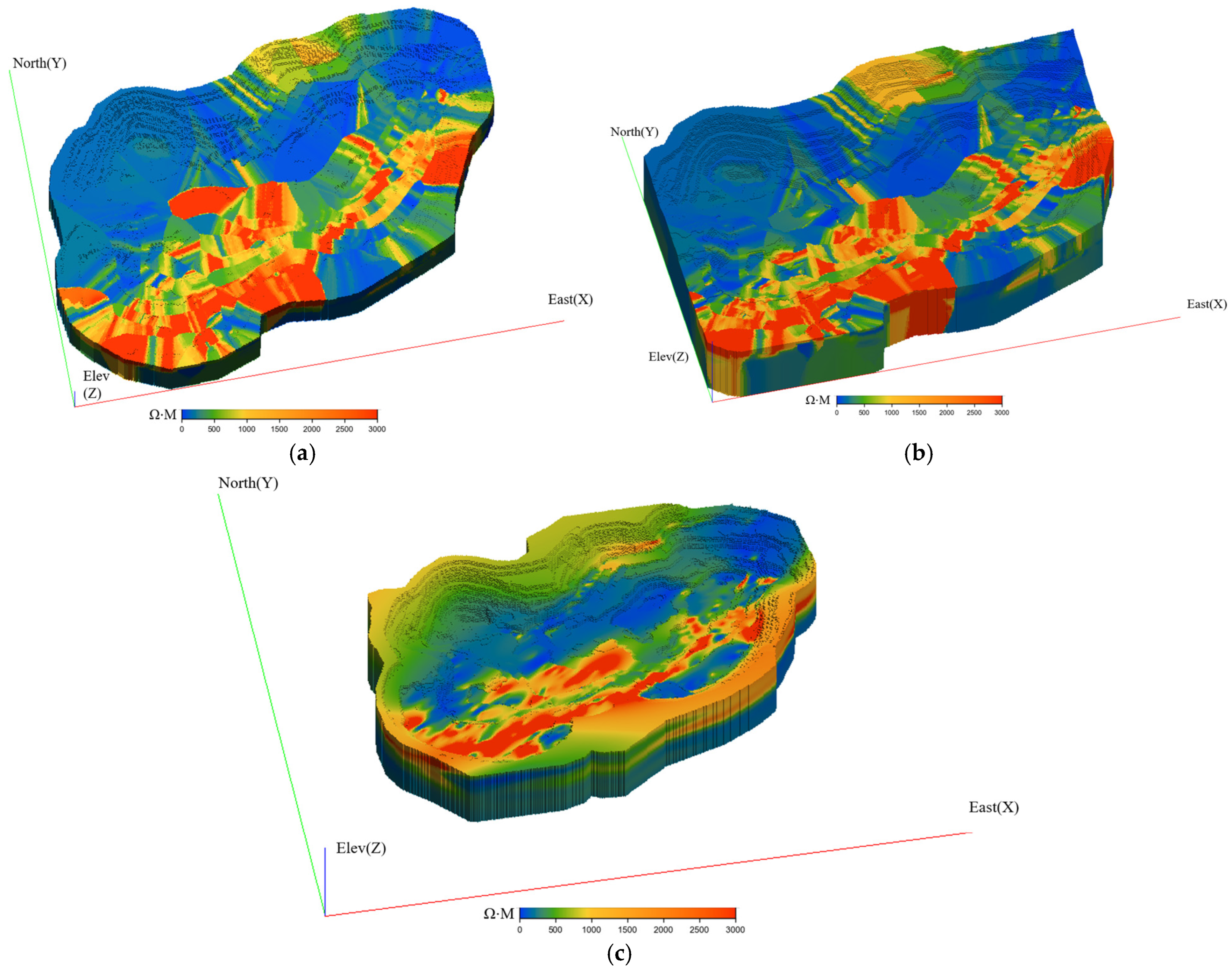
To evaluate the applicability of the spherical radial basis function interpolation method to three-dimensional resistivity model construction, its results were compared with those obtained using inverse distance weighting and linear radial basis function interpolation, as shown in Figure 6. For the inverse distance weighting interpolation, a search radius of 612 m was adopted, and the anisotropy ratios were set identical to those used in the spherical RBF method. Resistivity models were constructed using power parameters of 2 and 3, respectively. For the linear RBF interpolation, all parameter settings were identical to those of the spherical RBF method, except that the spherical kernel was replaced with a linear radial basis function kernel.

To compare the local interpolation performance of the different methods, random holdout validation was employed. A total of 2600 observed resistivity values were randomly selected as the validation set, while the remaining 29,364 observations were used for model construction. Each interpolation model was constructed using the same training and validation datasets, and the predicted values at the withheld locations were compared with the corresponding observations. The mean error (ME) and root mean square error (RMSE) were then calculated for each interpolation method. The validation results are presented in

Table 3. Results of random holdout validation.

Interpolation Methods	ME (Ω·m)	RMSE (Ω·m)
Spherical RBF	−12.2	299.0
Linear RBF	−7.3	351.7
IDW (P = 2)	13.9	383.2
IDW (P = 3)	29.7	346.0

.

Prediction errors were defined as $e_i={\widehat{\rho }}_i-{\rho }_i$, where ${\widehat{\rho }}_i$ and ${\rho }_i$ denote the predicted and observed resistivity values, respectively. The ME and RMSE were calculated on the original resistivity scale after inverse transformation as follows:

$$\mathrm{ME}={\displaystyle \frac{1}{n}}{\displaystyle \sum _{i=1}^n({\widehat{\rho }}_i-{\rho }_i)}$$

(19)

$$\mathrm{RMSE}=\sqrt{{\displaystyle \frac{1}{n}}{\displaystyle \sum _{i=1}^n{({\widehat{\rho }}_i-{\rho }_i)}^2}}$$

(20)

The random holdout validation results show that the spherical radial basis function (RBF) interpolation method yielded an ME of −12.2 Ω·m and an RMSE of 299.0 Ω·m. The relatively small absolute ME indicates that the model exhibits limited overall systematic bias. Its RMSE was the lowest among the four methods, representing reductions of approximately 15.0%, 22.0%, and 13.6% relative to linear RBF interpolation, IDW with $P=2$, and IDW with $P=3$, respectively. These results indicate that spherical RBF interpolation provides better local interpolation accuracy and overall error control within areas covered by existing measurements. However, because random holdout validation may place validation points close to training observations, spatial autocorrelation may lead to optimistic estimates of prediction error. Therefore, the reported ME and RMSE should be interpreted as measures of local interpolation performance under the current sampling configuration rather than as direct evidence of predictive accuracy in completely unsampled regions between survey lines. Overall, the compact support of the spherical kernel limits the influence of distant observations and suppresses unrealistic spatial propagation. Although its computational procedure is relatively complex, the spherical RBF method better preserves the continuity and smoothness of the resistivity field and is therefore more consistent with the objective of constructing a continuous three-dimensional resistivity model.

5. Conclusions

(1)

Through coordinate unification, elevation correction, quality control, and logarithmic transformation, the stability and comparability of the input data were improved. The resulting three-dimensional resistivity model constructed on this basis can clearly represent the spatial distribution and transitional relationships of high-, medium-, and low-resistivity zones within the study area, indicating that spherical RBF interpolation is suitable for three-dimensional continuous representation of resistivity properties in complex mining environments.

(2)

The incorporation of spatial anisotropy constraints enhances the model’s ability to characterize geological directional features. Semivariogram analysis reveals significant directional differences in the spatial continuity of log-transformed resistivity within the study area. By introducing anisotropic direction parameters and ellipsoidal axis ratios, the interpolation results exhibit strong continuity along the dominant geological structural orientation while suppressing unrealistic spatial spreading in subordinate directions, thereby producing a three-dimensional resistivity field that is more consistent with the structural and stratigraphic characteristics of the mining area.

(3)

In the random holdout validation, the spherical RBF method yielded an ME of −12.2 Ω·m and the lowest RMSE of 299.0 Ω·m, corresponding to RMSE reductions of 13.6–22.0% relative to linear RBF interpolation and the two IDW methods. These results demonstrate that the spherical RBF method provides better local interpolation performance within areas covered by existing measurements. However, because random holdout validation may be affected by spatial autocorrelation between the training and validation observations, the reported errors should not be interpreted as an independent assessment of predictive accuracy in completely unsampled regions. The compact support of the spherical kernel limits the influence of distant samples and suppresses unrealistic spatial propagation, thereby better preserving the continuity and smoothness of the resistivity field. The resulting model provides a continuous three-dimensional data basis for subsequent intelligent stratigraphic identification. Future work should incorporate borehole lithology, geological logging, and spatially independent observations to further evaluate model reliability.

(4)

The present study has not yet systematically evaluated the computational cost and scalability of the proposed method, although these factors are important for its practical application to large-scale mineral deposits. Future work will therefore employ datasets of different sizes under a unified hardware and software environment to quantitatively assess the method’s runtime, peak memory consumption, and performance variation with increasing data volume. These evaluations will clarify its computational feasibility and scalability for large-scale three-dimensional resistivity modeling and provide a basis for subsequent algorithm optimization and engineering applications.

References

1. Hasan, M.; Shang, Y.; Meng, H.; Shao, P.; Yi, X. Application of Electrical Resistivity Tomography (ERT) for Rock Mass Quality Evaluation. Sci. Rep. 2021, 11, 23683. [Google Scholar] [CrossRef] [Scilit] [PubMed]
2. Wang, Y.; Xue, G.; Han, J.; Luo, X.; Wang, B.; Ge, C.; Xu, H.; Guan, H.; Wang, Q.; Zhang, K.; et al. Progress in geophysical exploration of groundwater and its technical innovation. Geol. China 2025, 52, 1325–1351. [Google Scholar] [CrossRef]
3. Yang, B.; Zhang, X.; Liu, Z.; Xu, K. Technique and Application of Joint Magnetotelluric and Seismic Modeling and Constrained Inversion Based on Clustering and Multivariate Geostatistics. Oil Geophys. Prospect. 2021, 56, 670–677. [Google Scholar] [CrossRef]
4. Friedel, S. Resolution, stability and efficiency of resistivity tomography estimated from a generalized inverse approach. Geophys. J. Int. 2003, 153, 305–316. [Google Scholar] [CrossRef] [Scilit]
5. Dai, Q.; Xiao, B.; Feng, D. 3-D Inversion of the High Density Resistivity Method Based on Multi Profiles 2-D Exploration Data and Its Application. Geotech. Investig. Surv. 2011, 4, 84–89. [Google Scholar]
6. Meng, F.; Zhang, G.; Chen, M.; Li, H. 3-D Inversion of High Density Resistivity Method Based on 2-D High-Density Electrical Prospecting Data and Its Engineering Application. Geophys. Geochem. Explor. 2019, 43, 672–678. [Google Scholar] [CrossRef]
7. Hung, Y.; Lin, C.; Lee, C.; Weng, K. 3D and Boundary Effects on 2D Electrical Resistivity Tomography. Appl. Sci. 2019, 9, 2963. [Google Scholar] [CrossRef] [Scilit]
8. Mishra, U.; Bakshi, A.; Mandal, A. Enhanced 3D Visualization Based on Inverse Modeling of Non-Parallel 2D ERT Profiles: An Example for Assessing COPR Waste Dump Site in Umaran, India. J. Earth Syst. Sci. 2026, 135, 32. [Google Scholar] [CrossRef] [Scilit]
9. Jia, L.; Guo, X.; Zhang, F.; Huan, H. Fast Implementation of 3-D Visualization of High-Density Resistivity Data and Application in Complex Goaf Subsidence Areas. Geol. Resour. 2017, 26, 81–83. [Google Scholar] [CrossRef]
10. Chen, Y.; Fu, J.; Ma, H.; Zhu, Z. Research on Fault-Inclusive 3D Geological Implicit Modeling Method and Its Application. J. Jilin Univ. Earth Sci. Ed. 2025, 55, 1–12. [Google Scholar] [CrossRef]
11. Cui, M.; Hou, E.; Lu, T.; Hou, P.; Feng, D. Study on Spatial Interpolation Methods for High Precision 3D Geological Modeling of Coal Mining Faces. Appl. Sci. 2025, 15, 2959. [Google Scholar] [CrossRef] [Scilit]
12. Liu, X.; Zhang, P.; Guo, Y.; Ma, G.; Liu, M. Study of a High-Precision Complex 3D Geological Modelling Method Based on a Fine KNN and Kriging Coupling Algorithm: A Case Study for Jiangsu, China. Front. Earth Sci. 2023, 11, 1325907. [Google Scholar] [CrossRef] [Scilit]
13. Liu, H.; Chen, S.; Hou, M.; He, L. Improved Inverse Distance Weighting Method Application Considering Spatial Autocorrelation in 3D Geological Modeling. Earth Sci. Inform. 2020, 13, 619–632. [Google Scholar] [CrossRef] [Scilit]
14. Guo, J.; Wu, L.; Zhou, W. Automatic Ore Body Implicit 3D Modeling Based on Radial Basis Function Surface. J. China Coal Soc. 2016, 41, 2130–2135. [Google Scholar] [CrossRef]
15. Zhang, B.; Du, L.; Khan, U.; Tong, Y.; Wang, L.; Deng, H. AdaHRBF v1.0: Gradient-Adaptive Hermite–Birkhoff Radial Basis Function Interpolants for Three-Dimensional Stratigraphic Implicit Modeling. Geosci. Model. Dev. 2023, 16, 3651–3674. [Google Scholar] [CrossRef] [Scilit]
16. Hillier, M.J.; Schetselaar, E.M.; de Kemp, E.A.; Perron, G. Three-Dimensional Modelling of Geological Surfaces Using Generalized Interpolation with Radial Basis Functions. Math. Geosci. 2014, 46, 931–953. [Google Scholar] [CrossRef] [Scilit]
17. Qian, Z.; Zhang, J. Design of Slope Monitoring Scheme for Kambove Open-Pit Mine. Mod. Min. 2024, 40, 127–131. [Google Scholar] [CrossRef]
18. Dewaele, S.; Muchez, P.; Vets, J.; Fernandez-Alonzo, M.; Tack, L. Multiphase Origin of the Cu–Co Ore Deposits in the Western Part of the Lufilian Fold-and-Thrust Belt, Katanga (Democratic Republic of Congo). J. Afr. Earth Sci. 2006, 46, 455–469. [Google Scholar] [CrossRef] [Scilit]
19. Cailteux, J.L.H.; Muchez, P.; De Cuyper, J.; Dewaele, S.; De Putter, T. Origin of the megabreccias in the Katanga Copperbelt (D.R. Congo). J. Afr. Earth Sci. 2018, 140, 76–93. [Google Scholar] [CrossRef] [Scilit]
20. Kampunzu, A.B.; Cailteux, J. Tectonic Evolution of the Lufilian Arc (Central Africa Copper Belt) During Neoproterozoic Pan African Orogenesis. Gondwana Res. 1999, 2, 401–421. [Google Scholar] [CrossRef] [Scilit]
21. Li, C.; Wang, K.; Gao, Y.; Zheng, B.; Zhou, Y. Study on Hydrogeological Conditions and Mine Pit Water Inflow of the Main Ore Body in Kambove Mine. Min. Res. Dev. 2025, 45, 164–171. [Google Scholar] [CrossRef]
22. Wang, X. Based on the Three-Dimensional Expression of Pollutants in the Geological Model. Master’s Thesis, Anhui University of Science and Technology, Huainan, China, 7 December 2022. [Google Scholar]
23. Günther, T.; Rücker, C.; Spitzer, K. Three-Dimensional Modelling and Inversion of DC Resistivity Data Incorporating Topography—II. Inversion. Geophys. J. Int. 2006, 166, 506–517. [Google Scholar] [CrossRef] [Scilit]
24. Jia, Z.; Zhang, J.; Ding, S.; Feng, S.; Xiong, X.; Liang, G. Spatial Variation of Soil Phosphorus in Flooded Area of the Yellow River Based on GIS and Geo-Statistical Methods: A Case Study in Zhoukou City, Henan, China. Chin. J. Appl. Ecol. 2016, 27, 1211–1220. [Google Scholar] [CrossRef] [PubMed]
25. Yang, Z.; Chen, X.; Jing, F.; Guo, B.; Lin, G. Spatial Variability of Nutrients and Heavy Metals in Paddy Field Soils Based on GIS and Geostatistics. Chin. J. Appl. Ecol. 2018, 29, 1893–1901. [Google Scholar] [CrossRef] [PubMed]
26. Zhao, S. Research on Technologies of Digital Mining Models and Optimization for Underground Metal Mines. Ph.D. Thesis, Central South University, Changsha, China, 2025. [Google Scholar]
27. Faiyaz, C.A.; Shahrear, P.; Shamim, R.A.; Strauss, T.; Khan, T. Comparison of different radial basis function networks for the electrical impedance tomography (EIT) inverse problem. Algorithms 2023, 16, 461. [Google Scholar] [CrossRef] [Scilit]
28. Wang, W.; Zhou, J.; Wang, S.; Li, X. Research on Three-Dimensional Modeling of Strata Block Based on Radial Basis Function. Rock Soil Mech. 2012, 33, 939–944. [Google Scholar] [CrossRef]
Figure 1. High-density resistivity data preprocessing flowchart.
Applsci 16 07736 g001
Figure 2. Distribution map of preprocessed resistivity data.
Applsci 16 07736 g002
Figure 3. Distribution map of resistivity data before and after logarithmic transformation. (a) Resistivity data distribution map; (b) Resistivity data distribution map after logarithmic transformation. The red diamond indicates the arithmetic mean.
Applsci 16 07736 g003
Figure 4. Semivariogram curve under spherical model. (a) Semivariogram plot in the major axis direction; (b) semivariogram in the semi-major axis direction; (c) semivariogram in the minor axis directions. The blue dots represent the experimental semivariogram values, and the blue solid lines represent the fitted theoretical semivariogram models.
Applsci 16 07736 g004
Figure 5. Resistivity model constructed using spherical radial basis function interpolation.
Applsci 16 07736 g005
Figure 6. Resistivity models obtained from different methods. (a) Resistivity model by inverse distance weighting (power = 2); (b) resistivity model by inverse distance weighting (power = 3); (c) resistivity model by linear RBF interpolation.
Applsci 16 07736 g006