Airy Stress Function-Based Elastoplastic Analysis of Plates with Holes Using the Nonconforming Morley Finite Element Method

Abstract

This paper presents a stress-function-based finite element formulation for two-dimensional elastoplastic plane-stress problems with holes. The Airy stress function is used as the primary global unknown, and the resulting non-homogeneous biharmonic equation is discretized with the nonconforming Morley finite element. The stresses are obtained from the second derivatives of the discrete Airy function. Consequently, the differential equilibrium equations are satisfied inside each element, while interelement coupling is enforced through the Morley weak formulation. Plastic strains enter the governing equation through an element-wise weak-form contribution, which avoids the direct evaluation of their second derivatives. The local material response is described by associated von Mises plasticity with Kuhn–Tucker conditions and is integrated using cutting-plane and return-mapping algorithms. The formulation is applied to a perforated plate subjected to in-plane tension and compared with a classical displacement-based elastoplastic finite element model. The results show good agreement in the elastic stress concentration, yielding load, stress redistribution, and plastic-zone development. For the present benchmark, the Airy–Morley formulation is computationally competitive and provides a stress-function-based alternative for a restricted class of two-dimensional plane-stress problems.

1. Introduction

Plates with holes are classical examples of stress concentration problems. Stress concentration remains an active topic in modern solid mechanics extending beyond idealized holes: for example, in problems involving surface irregularities and local geometric defects [1]. The stress field near a hole is strongly non-uniform and may lead to local yielding even under moderate remote loading. For this reason, perforated plates are useful benchmarks for numerical methods in plane-stress elasticity and elastoplasticity [2]. In this paper, the word “plate” is used in the sense of a thin body subjected to in-plane loading. Thus, the problem is a plane-stress problem, not a plate-bending problem.

In engineering practice, such problems are usually solved by displacement-based finite element methods (FEM). This is also the standard setting in general-purpose commercial solid-mechanics solvers [3,4,5]. The nodal displacements are the primary unknowns, and the strains and stresses are computed later from the displacement field and the constitutive law. This approach is general and efficient. However, the recovered stress field is not the primary unknown of the global problem. As a result, equilibrium is satisfied only in the weak displacement sense, while stresses are obtained as post-processed quantities.

An alternative approach, which is particularly useful when stress concentrations are the main quantities of interest, is to use stresses or stress functions as the primary variables [6,7]. In two-dimensional elasticity, the Airy stress function provides a classical way to represent stress fields that satisfy equilibrium equations identically. The Airy representation enforces the differential equilibrium equations within each element, whereas interelement coupling is provided by the nonconforming Morley weak formulation. This idea goes back to Airy, who introduced a scalar function to describe internal stress and strain states in beams and related elastic bodies [8]. In modern notation, the Airy stress function Φ(x,y) gives the in-plane stresses by second derivatives of Φ. Therefore, equilibrium is built into the stress representation.

Morley developed variational methods for plane elasticity using the Airy stress function and emphasized that the Airy formulation and plate-bending formulations are closely related because both lead to fourth-order equations [9]. This observation is important for the present work. It means that a numerical method designed for biharmonic problems can also be used for plane-stress problems written in terms of the Airy stress function.

The Morley finite element is a natural candidate for this purpose. It is a nonconforming quadratic triangular element with degrees of freedom given by function values at vertices and normal derivatives at edge midpoints. It was originally developed in the context of plate bending and equilibrium finite elements [10]. From the finite element point of view, the Morley element is much simpler than conforming C¹ elements such as the Argyris element, whose implementation requires high-order interpolation and many nodal derivatives. This difficulty has also motivated alternative C⁰, nonconforming, and continuous/discontinuous discretizations for fourth-order problems [11,12]. Recent developments in higher-continuity finite element approximations, including B-spline-based formulations, also show that increasing interelement continuity remains an active research direction. However, the present work intentionally uses the simpler nonconforming Morley element [13]. The mathematical theory of nonconforming finite elements also identifies the Morley element as a standard tool for biharmonic problems [14].

Stress-based and equilibrium-based finite element methods have a long history. Křížek studied conforming equilibrium FEM for several plane elliptic problems, including linear elasticity and biharmonic problems, using stream functions and the Airy function [15]. Vallabhan and Azene used the Airy stress function in a complementary energy finite element formulation for plane elasticity, obtaining self-equilibrated stresses directly from the stress function [16]. These works show that Airy-based stress formulations are well established in elasticity. However, such formulations are usually more involved than displacement-based FEM, especially when boundary conditions and compatibility constraints are treated in a fully conforming way.

The relation between elasticity, Stokes flow, and biharmonic FEM was also studied by Falk and Morley. They showed that several finite element methods for elasticity and Stokes equations can be reduced to modified Morley methods for the biharmonic equation by elimination procedures analogous to those used in the continuous theory [17]. This supports the view that the Morley element is not only a plate-bending element, but also a useful discrete tool for scalar biharmonic formulations arising from plane elasticity.

The present paper extends this idea to small-strain elastoplastic plane stress. Previous Airy-based $J_2$ formulations lead to a non-homogeneous biharmonic equation with a source term containing derivatives of plastic strains [18]. In the proposed method, the Airy stress function is discretized using the nonconforming Morley element and the plastic source term is introduced in weak form. This transfers the derivatives to the test functions and avoids explicit differentiation of the element-wise plastic strain field.

The present work makes three main contributions. First, the elastoplastic plane-stress problem is formulated in terms of the Airy stress function, leading to a non-homogeneous biharmonic equation with a plastic-strain source term. Second, a Morley finite element discretization is derived in weak form, so that the plastic contribution is assembled as an element-wise right-hand side. Third, the method is tested on a perforated plate subjected to in-plane tension and compared with a classical displacement-based elastoplastic finite element solution.

The paper is organized as follows. Section 2 presents the governing equations and the Airy stress function formulation for plane-stress elastoplasticity. Section 3 derives the weak form and the Morley finite element discretization. Section 4 describes the local cutting-plane and return-mapping algorithms used for the plastic update. Section 5 presents the classical displacement-based finite element model used for comparison. Section 6 discusses numerical results for a plate with a circular hole. Final conclusions are given in Section 7.

2. Governing Equations and Airy-Stress Function Formulation

Let $\Omega \subset {\mathbb{R}}^2$ be a plane-stress domain with boundary Γ. The in-plane coordinates are denoted by $x_{\alpha }$, where $\alpha =1, 2$. Greek indices take the values 1 and 2, and the summation convention is used. A comma denotes partial differentiation, for example a $a_{\alpha ,\beta }={\displaystyle \frac{\partial a_{\alpha }}{\partial x_{\beta }}}$.

Body forces are neglected. The local equilibrium equations are

$${\sigma }_{\alpha \beta ,\beta }=0\hspace{1em}\mathrm{in}\hspace{0.33em}\Omega ,$$

(1)

On the boundary, the traction vector is

$${\overline{t}}_{\alpha }={\sigma }_{\alpha \beta }{n}_{\beta }\hspace{1em}\mathrm{on}\hspace{0.33em}\Gamma$$

(2)

where $n_{\beta }$ is the outward unit normal vector. The small strain tensor is

$${\epsilon }_{\alpha \beta }={\displaystyle \frac{1}{2}}\left(u_{\alpha ,\beta }+u_{\beta ,\alpha }\right)$$

(3)

where $u_{\alpha }$ is the displacement vector. The in-plane compatibility condition is written as

$$2{\epsilon }_{\mathrm{12,12}}-{\epsilon }_{\mathrm{11,22}}-{\epsilon }_{\mathrm{22,11}}=0$$

(4)

The total strain is decomposed into elastic and plastic parts:

$${\epsilon }_{\alpha \beta }={\epsilon }_{\alpha \beta }^e+{\epsilon }_{\alpha \beta }^p$$

(5)

For plane stress, ${\sigma }_{33}=0$, ${\sigma }_{\alpha 3}=0$. The plane-stress constitutive relation is

$${\epsilon }_{\alpha \beta }={\displaystyle \frac{1+\nu }{E}}{\sigma }_{\alpha \beta }-{\displaystyle \frac{\nu }{E}}{\sigma }_{\gamma \gamma } {\delta }_{\alpha \beta }+{\epsilon }_{\alpha \beta }^p$$

(6)

where $E$ is Young’s modulus, $\nu$ is Poisson’s ratio, and ${\delta }_{\alpha \beta }$ is the Kronecker delta. The plastic strain is assumed to be incompressible. Hence,

$${\epsilon }_{33}^p=-\left({\epsilon }_{11}^p+{\epsilon }_{22}^p\right)$$

(7)

The plane-stress von Mises equivalent stress is

$${\sigma }_{\mathrm{eq}}=\sqrt{{\sigma }_{11}^2-{\sigma }_{11}{\sigma }_{22}+{\sigma }_{22}^2+3{\sigma }_{12}^2}$$

(8)

The yield function is

$$f\left(\sigma ,\kappa \right)={\sigma }_{\mathrm{eq}}-{\sigma }_Y\left(\kappa \right)$$

(9)

where $\kappa$ is the scalar hardening variable. For linear isotropic hardening,

$${\sigma }_Y\left(\kappa \right)={\sigma }_{Y0}+H\kappa$$

(10)

Here, ${\sigma }_{Y0}$ is the initial yield stress and $H$ is the hardening modulus. Perfect plasticity is obtained for $\mathrm{H} = 0$. The associated flow rule is written as

$${\dot{\epsilon }}_{\alpha \beta }^p=\lambda {\displaystyle \frac{\partial f}{\partial {\sigma }_{\alpha \beta }}}$$

(11)

where $\lambda$ denotes the plastic multiplier. The Kuhn–Tucker conditions are

$$\lambda \ge 0,\hspace{1em}f\left(\sigma ,\kappa \right)\le 0,\hspace{1em}\lambda f\left(\sigma ,\kappa \right)=0$$

(12)

The Airy stress function $\Phi =\Phi \left(x_1,x_2\right)$ is introduced by

$${\sigma }_{11}={\Phi }_{,22},\hspace{1em}{\sigma }_{22}={\Phi }_{,11},\hspace{1em}{\sigma }_{12}=-{\Phi }_{,12}$$

(13)

This representation satisfies Equation (1) identically. Substitution of the plane-stress constitutive Equation (6) into the compatibility condition (4) gives

$$2{\left({\displaystyle \frac{1+\nu }{E}}{\sigma }_{12}+{\epsilon }_{12}^p\right)}_{,12}-{\left[{\displaystyle \frac{1}{E}}\left({\sigma }_{11}-\nu {\sigma }_{22}\right)+{\epsilon }_{11}^p\right]}_{,22}-{\left[{\displaystyle \frac{1}{E}}\left({\sigma }_{22}-\nu {\sigma }_{11}\right)+{\epsilon }_{22}^p\right]}_{,11}=0$$

(14)

After substituting Equation (13) into Equation (14), the terms containing Poisson’s ratio cancel. Rearranging the plastic-strain terms gives the non-homogeneous biharmonic equation

$${𝛻}^{ 4} \Phi =E\left(2{\epsilon }_{\mathrm{12,12}}^p-{\epsilon }_{\mathrm{11,22}}^p-{\epsilon }_{\mathrm{22,11}}^p\right)$$

(15)

The plastic-strain derivatives in Equation (15) are subsequently transferred to the test function in the weak formulation derived in Section 3. Here,

$${𝛻}^{ 2} \Phi :={\Phi }_{,11}+{\Phi }_{,22}\mathrm{and} {𝛻}^{ 4} \Phi :={\Phi }_{,1111}+2{\Phi }_{,1122}+{\Phi }_{,2222}$$

(16)

The stress field is unchanged if an affine function is added to $\Phi$

$${\Phi }^{*}=\Phi +a x_1+b x_2+c$$

(17)

because ${\Phi }_{, \alpha \beta }^{*}={\Phi }_{, \alpha \beta }$. This property is used in the treatment of traction-free holes.

Although the preceding formulation is general, the present paper focuses on perforated rectangular domains subjected to uniform remote tension. Therefore, the Airy boundary conditions are specialized here to the loading case used later in the numerical study. For a remote uniform tensile stress $p$ in the $x_1$ direction, the external Airy field is chosen as (see Figure 1a)

$${\Phi }_0\left(x_1,x_2\right)={\displaystyle \frac{p}{2}}{x}_2^2$$

(18)

This field gives ${\sigma }_{11}=p$, ${\sigma }_{22}=0$, ${\sigma }_{12}=0$. Thus, on the external boundary ${\Gamma }_{ext}$, the following conditions are imposed:

$$\Phi ={\Phi }_0,\hspace{1em}{\Phi }_{,n}={\Phi }_{0,n}$$

(19)

The normal derivative is ${\Phi }_{,n}={\Phi }_{,\alpha }{n}_{\alpha }$. For ${\Phi }_0$, this gives ${\Phi }_{0,n}=p x_2 n_2$. On a traction-free hole boundary ${\Gamma }_h$, the Airy function is taken in affine form,

$$\Phi =a x_1+b x_2+c\hspace{1em}\mathrm{on}\hspace{0.33em}{\Gamma }_h$$

(20)

with

$${\Phi }_{,n}=a n_1+b n_2\hspace{1em}\mathrm{on}\hspace{0.33em}{\Gamma }_h$$

(21)

The coefficients $a$ and $b$ define the constant gradient of $\Phi$ on the hole boundary, while $c$ defines its level. A common affine addition does not change the stresses, but the relative affine data on different boundary components are determined by three compatibility conditions per hole. These conditions ensure closure of the two displacement components and the rotation around the hole.

The strong Airy problem used in this work consists of Equation (15) in $\Omega$, completed by Equation (19) on ${\Gamma }_{ext}$ and Equations (20) and (21) on ${\Gamma }_h$. The affine coefficients associated with each hole are determined by the global variational equations, which enforce the additional compatibility conditions required in a multiply connected domain.

3. Weak Form and Morley Finite Element Discretization

The weak form is obtained by multiplying Equation (15) by an admissible test function $\eta$ and integrating it over $\Omega$ [19,20].

$${\int }_{\Omega }{𝛻}^4\Phi \eta \mathrm{d}\Omega =E{\int }_{\Omega }\left(2{\epsilon }_{\mathrm{12,12}}^p-{\epsilon }_{\mathrm{11,22}}^p-{\epsilon }_{\mathrm{22,11}}^p\right) \eta \mathrm{d}\Omega$$

(22)

After integration by parts in the admissible Airy space, with homogeneous variations on the prescribed external boundary and admissible affine variations on traction-free holes, the weak form is

$${\int }_{\Omega }{\Phi }_{,\alpha \beta } {\eta }_{,\alpha \beta } \mathrm{d}\Omega =E{\int }_{\Omega }\left(2{\epsilon }_{12}^p {\eta }_{,12}-{\epsilon }_{11}^p {\eta }_{,22}-{\epsilon }_{22}^p {\eta }_{,11}\right) \mathrm{d}\Omega$$

(23)

The left-hand side of Equation (23) means

$${\Phi }_{,\alpha \beta } {\eta }_{,\alpha \beta }={\Phi }_{,11} {\eta }_{,11}+2 {\Phi }_{,12} {\eta }_{,12}+{\Phi }_{,22} {\eta }_{,22}$$

(24)

Thus, the weak problem can be written as follows:

$$a\left(\Phi ,\eta \right)=l^p\left(\eta \right)\hspace{1em}\forall \eta$$

(25)

where

$$a\left(\Phi ,\eta \right)={\int }_{\Omega }{\Phi }_{,\alpha \beta } {\eta }_{,\alpha \beta } \mathrm{d}\Omega$$

(26)

and

$$l^p\left(\eta \right)=E{\int }_{\Omega }\left(2{\epsilon }_{12}^p {\eta }_{,12}-{\epsilon }_{11}^p {\eta }_{,22}-{\epsilon }_{22}^p {\eta }_{,11}\right) \mathrm{d}\Omega$$

(27)

This form is used because derivatives are transferred from ${\epsilon }_{\alpha \beta }^p$ to the test function. Therefore, the numerical scheme does not require direct computation of ${\epsilon }_{\alpha \beta ,\gamma \delta }^p$.

3.1. Morley Finite Element Approximation

Let the finite element mesh be denoted by ${\mathcal{T}}_h={\left\{ {\Omega }_e\right\}}_{e=1}^{n_{ el}}$, where ${\Omega }_e$ is the $e$-th triangular element and $n_{el}$ is the number of elements. The element area is denoted by $A_e$. On each element ${\Omega }_e$, the Airy stress function is approximated by a quadratic polynomial

$${\Phi }_h{|}_{ {\Omega }_e}=c_0^{\left(e\right)}+c_{\alpha }^{\left(e\right)}{x}_{\alpha }+{\displaystyle \frac{1}{2}}{c}_{\alpha \beta }^{\left(e\right)} x_{\alpha } x_{\beta },\hspace{1em}{c}_{\alpha \beta }^{\left(e\right)}=c_{\beta \alpha }^{\left(e\right)}$$

(28)

Therefore, ${\Phi }_{h,\alpha \beta }{|}_{ {\Omega }_e}=c_{\alpha \beta }^{\left(e\right)}$.

The Morley element has six local degrees of freedom. The first three are the values of ${\Phi }_h$ at the vertices $z_r^{\left(e\right)}$:

$$d_r^{ \left(e\right)}\left({\Phi }_h\right)={\Phi }_h\left(z_r^{\left(e\right)}\right),\hspace{1em}r=1,\hspace{0.33em}2,\hspace{0.33em}3$$

(29)

The remaining three degrees of freedom are normal derivatives at the edge midpoints $m_{ r}^{\left(e\right)}$:

$$d_{3+r}^{ \left(e\right)}\left({\Phi }_h\right)={\Phi }_{h,\alpha }\left(m_r^{\left(e\right)}\right)n_{\alpha }^{(e,r)},\hspace{1em}r=1,\hspace{0.33em}2,\hspace{0.33em}3$$

(30)

Here, $n_{\alpha }^{(e,r)}$ is the unit normal vector assigned to the $r$-th edge.

The Morley space is nonconforming. Its functions are quadratic on each element, are continuous at vertices, and have single-valued normal derivatives at edge midpoints.

3.2. Discrete Weak Form

The Morley discretization is obtained by restricting the continuous weak form to the nonconforming space $M_h$. Since $M_h\not\subset H^2\left(\Omega \right)$, the second derivatives are evaluated element-wise. Therefore, the continuous bilinear form (see (26)) is replaced by

$$a_h\left({\Phi }_h,{\eta }_h\right)=\sum _{e=1}^{n_{e l}}{\int }_{{\Omega }_e}{{\Phi }_h}_{,\alpha \beta } {\eta }_{h,\alpha \beta } \mathrm{d}\Omega$$

(31)

Similarly, the plastic-strain contribution is written as (compare Equation (27))

$$l_h^p\left({\eta }_h\right)=E\sum _{e=1}^{n_{e l}}{\int }_{{\Omega }_e}\left(2{\epsilon }_{12}^{p,h}{\eta }_{h,12}-{\epsilon }_{11}^{p,h}{\eta }_{h,22}-{\epsilon }_{22}^{p,h}{\eta }_{h,11}\right) \mathrm{d}\Omega$$

(32)

The discrete problem is therefore as follows: find ${\Phi }_h\in M_h$, satisfying the imposed Airy boundary conditions, such that

$$a_h\left({\Phi }_h,{\eta }_h\right)=l_h^p\left({\eta }_h\right)\hspace{1em}\forall {\eta }_h\in M_h^0$$

(33)

Here, $M_h^0$ denotes the Morley test space with homogeneous Airy data on the prescribed external boundary and admissible affine variations in traction-free holes.

3.3. Element Stiffness Matrix

On element ${\Omega }_e$, the local Morley approximation is written as

$${\Phi }_h{|}_{{\Omega }_e}=a_J^{\left(e\right)}{\phi }_J^{\left(e\right)},\hspace{1em}J=1,\dots ,6$$

(34)

Here, ${\phi }_J^{\left(e\right)}$ are the local Morley basis functions and $a_J^{\left(e\right)}$ are the local degrees of freedom. Since ${\phi }_J^{\left(e\right)}$ are quadratic polynomials, their second derivatives are constant on ${\Omega }_e$. The element stiffness matrix is therefore

$$k_{IJ}^{\left(e\right)}={\int }_{{\Omega }_e}{\phi }_{J,\alpha \beta }^{\left(e\right)}{\phi }_{I,\alpha \beta }^{\left(e\right)} \mathrm{d} \Omega =A_{ e}{\phi }_{J,\alpha \beta }^{\left(e\right)}{\phi }_{I,\alpha \beta }^{\left(e\right)}$$

(35)

In expanded form

$$k_{IJ}^{\left(e\right)}=A_e\left({\phi }_{J,11}^{\left(e\right)} {\phi }_{I,11}^{\left(e\right)}+2 {\phi }_{J,12}^{\left(e\right)} {\phi }_{I,12}^{\left(e\right)}+{\phi }_{J,22}^{\left(e\right)} {\phi }_{I,22}^{\left(e\right)}\right)$$

(36)

3.4. Element Plastic Load Vector

The element load vector generated by the plastic strain field is

$$f_I^{p,\left(e\right)}=E{\int }_{{\Omega }_e}\left(2{\epsilon }_{12}^{p,h}{\phi }_{I,12}^{\left(e\right)}-{\epsilon }_{11}^{p,h}{\phi }_{I,22}^{\left(e\right)}-{\epsilon }_{22}^{p,h}{\phi }_{I,11}^{\left(e\right)}\right)\mathrm{d}\Omega$$

(37)

In the present implementation, the plastic strain is assumed to be constant on each element. Thus, the element vector reduces to

$$f_I^{p,\left(e\right)}=E{A}_e\left(2{\epsilon }_{12,e}^p {\phi }_{I,12}^{\left(e\right)}-{\epsilon }_{11,e}^p {\phi }_{I,22}^{\left(e\right)}-{\epsilon }_{22,e}^p {\phi }_{I,11}^{\left(e\right)}\right)$$

(38)

3.5. Global System and Boundary Constraints

The element matrices and plastic load vectors are assembled into the global stiffness matrix $\mathit{K}$ and the global vector ${\mathit{f}}^p$. The resulting algebraic system is

$$\mathit{K} \mathit{a}={\mathit{f}}^p$$

(39)

where $\mathit{a}$ contains all global Morley degrees of freedom. It contains the values of ${\Phi }_h$ at mesh vertices and the normal derivatives of ${\Phi }_h$ at edge midpoints.

The external boundary conditions prescribe selected components of $\mathit{a}$. The degrees of freedom at each traction-free hole are related through the affine representation of the Airy function. Consequently, the components of $\mathit{a}$ are not independent. Every admissible vector is represented as

$$\mathit{a}={\mathit{a}}^0+\mathit{P} \mathit{z}$$

(40)

The vector ${\mathit{a}}^0$ contains the prescribed values of ${\Phi }_h$ and ${\Phi }_{h,n}$ on the external boundary. The vector $\mathit{z}$ contains the independent unknowns: the free Morley degrees of freedom and the affine coefficients associated with the hole boundaries. The matrix $\mathit{P}$ is the constraint transformation matrix that maps $\mathit{z}$ to the complete vector $\mathit{a}$.

Substitution of this representation into the assembled equations and projection onto the independent degrees of freedom gives

$${\mathit{P}}^T\mathit{K} \mathit{P} \mathit{z}={\mathit{P}}^T\left({\mathit{f}}^p-\mathit{K} {\mathit{a}}^0\right)$$

(41)

This is the system solved numerically for $\mathit{z}$. The complete Airy solution is then obtained from Equation (40). External loading enters through the load-dependent boundary vector ${\mathit{a}}^0$, whereas the current plastic strain field enters through ${\mathit{f}}^p$.

In matrix $\mathit{P}$, three columns per hole correspond to $\mathit{a}$, $\mathit{b}$ and $\mathit{c}$. Therefore, projection in Equation (41) introduces three additional equations that enforce these global compatibility conditions.

3.6. Stress Recovery

Using the local quadratic approximation introduced in Section 3.1, the stress components are recovered directly from the Airy stress function.

$${\sigma }_{11}^{\left(e\right)}={\Phi }_{h,22}{|}_{ {\Omega }_e},\hspace{1em}{\sigma }_{22}^{\left(e\right)}={\Phi }_{h,11}{|}_{ {\Omega }_e},\hspace{1em}{\sigma }_{12}^{\left(e\right)}=-{\Phi }_{h,12}{|}_{ {\Omega }_e}$$

(42)

Because the Morley approximation is quadratic on each element, the recovered stresses are constant within ${\Omega }_e$. These element stresses are used directly in the local elastoplastic update. Area-weighted nodal values are calculated only for visualization.

4. Local Integration of the Elastoplastic Model

The local constitutive update follows standard algorithms for rate-independent associated plasticity. No new material integration method is introduced in this work. The cutting-plane and return-mapping procedures are used as alternative local solvers [21,22,23,24].

At each global iteration, an element strain estimate is reconstructed from the current stress and plastic strain,

$${\epsilon }_{\alpha \beta }^{\left(k\right)}=S_{\alpha \beta \gamma \delta }^{ \mathrm{ps}} {\sigma }_{\gamma \delta }^{\left(k\right)}+{\epsilon }_{\alpha \beta }^{p,\left(k\right)}$$

(43)

where $S_{\alpha \beta \gamma \delta }^{ \mathrm{ps}}$ is the plane-stress elastic compliance tensor and $k$ denotes the current global iteration. Using the plastic strain and hardening variable from the previous converged load step $n$, the elastic trial stress is

$${\sigma }_{\alpha \beta }^{\mathrm{tr}}=C_{\alpha \beta \gamma \delta }^{ \mathrm{ps}}\left({\epsilon }_{\gamma \delta }^{\left(k\right)}-{\epsilon }_{\gamma \delta }^{p,n}\right)$$

(44)

where $C_{\alpha \beta \gamma \delta }^{ \mathrm{ps}}$ is the plane-stress elastic stiffness tensor. If $f^{\mathrm{tr}}=f\left({\sigma }_{\alpha \beta }^{\mathrm{tr}},{\kappa }^n\right)\le 0$, the step is elastic and the internal variables remain unchanged.

4.1. Cutting-Plane Update

If $f^{\mathrm{tr}}>0$, the cutting-plane algorithm applies successive linearized corrections. At local iteration $j$, the correction of the plastic multiplier is

$$\delta {\lambda }^{\left(j\right)}={\displaystyle \frac{f\left({\sigma }_{\alpha \beta }^{\left(j\right)},{\kappa }^{\left(j\right)}\right)}{n_{\alpha \beta }^{\left(j\right)}{C}_{\alpha \beta \gamma \delta }^{ \mathrm{ps}} n_{\gamma \delta }^{\left(j\right)}+H}}$$

(45)

where

$$n_{\alpha \beta }^{\left(j\right)}={\left.{\displaystyle \frac{\partial f}{\partial {\sigma }_{\alpha \beta }}}\right|}_{{\sigma }^{\left(j\right)}}$$

(46)

The plastic strain and the hardening variable are updated as follows:

$${\epsilon }_{\alpha \beta }^{p,(j+1)}={\epsilon }_{\alpha \beta }^{p,\left(j\right)}+\delta {\lambda }^{\left(j\right)}{n}_{\alpha \beta }^{\left(j\right)}\hspace{0.33em},\hspace{1em}{\kappa }^{(j+1)}={\kappa }^{\left(j\right)}+\delta {\lambda }^{\left(j\right)}$$

(47)

The stress is recalculated from the constitutive relation, and the correction is repeated until the yield condition is satisfied.

4.2. Return-Mapping Update

The implicit return-mapping algorithm solves directly for the updated stress and the total plastic multiplier increment, $\mathsf{\Delta }\lambda$. The local residual equations are

$$r_{\alpha \beta }={\sigma }_{\alpha \beta }^{n+1}-{\sigma }_{\alpha \beta }^{\mathrm{tr}}+\mathsf{\Delta }\lambda C_{\alpha \beta \gamma \delta }^{ \mathrm{ps}} n_{\gamma \delta }^{n+1}=0$$

(48)

and

$$r_f=f\left({\sigma }_{\alpha \beta }^{n+1},{\kappa }^n+\mathsf{\Delta }\lambda \right)=0$$

(49)

This nonlinear system is solved using a local Newton iteration. After convergence, the internal variables are updated from

$${\epsilon }_{\alpha \beta }^{p,n+1}={\epsilon }_{\alpha \beta }^{p,n}+\mathsf{\Delta }\lambda n_{\alpha \beta }^{n+1},\hspace{1em}{\kappa }^{n+1}={\kappa }^n+\mathsf{\Delta }\lambda$$

(50)

The updated element plastic strains are used to assemble a new vector ${\mathit{f}}^p$. The global Airy problem and the local constitutive updates are repeated until both the plastic strain field and the yield condition converge.

5. Classical Displacement-Based FEM Model

A conventional displacement-based finite element model is used as a reference solution. The displacement field $u_{\alpha }$ is the primary unknown, and the strain tensor is obtained from Equation (23). The weak form of equilibrium is

$${\int }_{\Omega }{\sigma }_{\alpha \beta } {\epsilon }_{\alpha \beta }\left(\eta \right) \mathrm{d} \Omega ={\int }_{{\Gamma }_t}{\overline{t}}_{\alpha } {\eta }_{\alpha } \mathrm{d} \Gamma$$

(51)

where

$${\epsilon }_{\alpha \beta }\left(\eta \right)={\displaystyle \frac{1}{2}}\left({\eta }_{\alpha ,\beta }+{\eta }_{\beta ,\alpha }\right)$$

(52)

Here, ${\eta }_{\alpha }$ is an admissible test displacement and ${\overline{t}}_{\alpha }$ is the prescribed traction on boundary traction part ${\Gamma }_t$. This is the standard displacement formulation of the finite element method [25,26].

The domain is discretized using three-node triangular elements. The displacement and strain approximations on element ${\Omega }_e$ are

$$u_{\alpha ,h}=N_I u_{\alpha I}\hspace{0.33em},\hspace{1em}{\epsilon }_{\alpha \beta ,h}=B_{\alpha \beta I\gamma }{u}_{\gamma I}$$

(53)

where $N_I$ are the element shape functions and $B_{\alpha \beta I\gamma }$ is the strain-displacement operator. At each load step, stresses and plastic variables are updated element-wise using the same plane-stress constitutive model and the same local integration algorithms as in Section 4. The global non-linear equations are written as

$$\mathit{r}={\mathit{f}}_{\mathrm{ext}}-{\mathit{f}}_{\mathrm{int}}=0$$

(54)

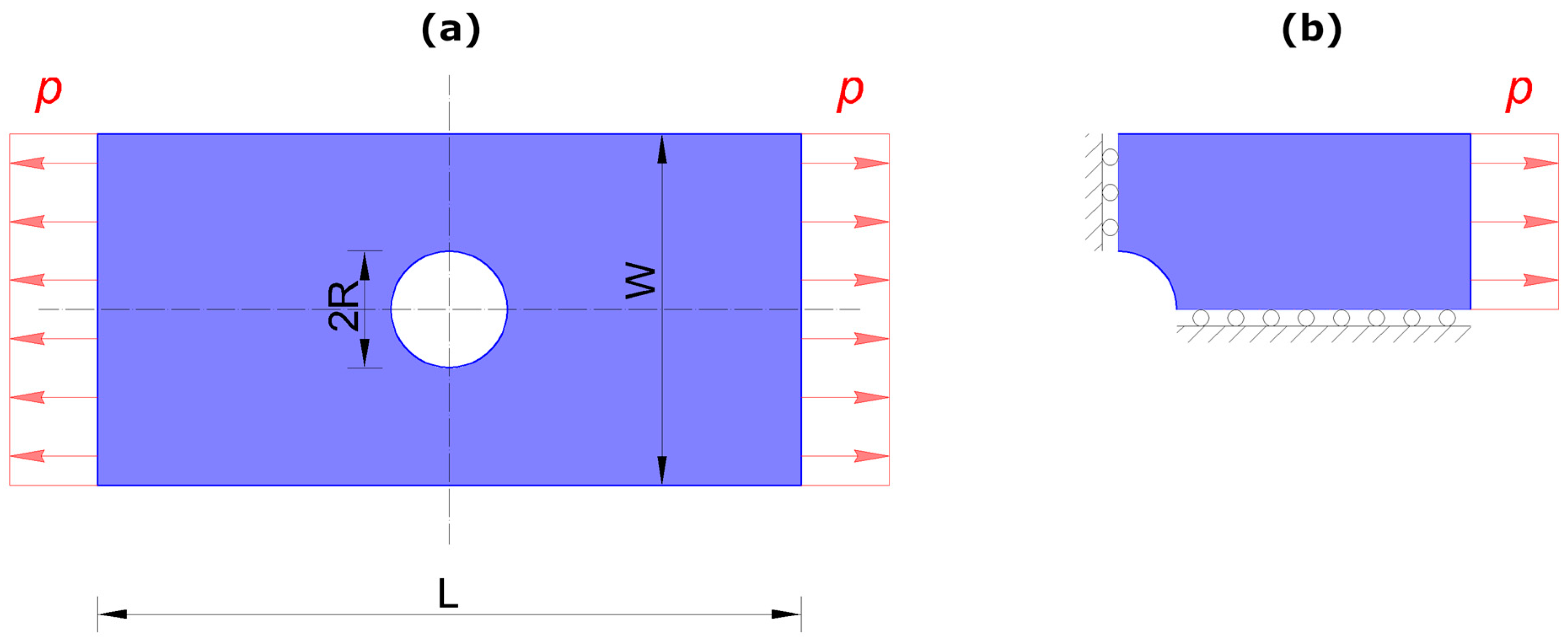
The comparison model uses one quarter of the perforated domain (see Figure 1b). Symmetry conditions are imposed along the coordinate axes, while the external traction is applied to the outer boundary. The same geometry, material parameters, loading history, and local plasticity model are used in both formulations. Thus, the comparison isolates the influence of the global formulation: displacement-based equilibrium in the reference model and Airy stress-function-based equilibrium in the proposed method.

6. Numerical Results

The analyzed geometry and boundary conditions are shown in Figure 1. A rectangular plate with a central circular hole is subjected to uniform tensile traction $p$ applied to its vertical external boundaries. The horizontal external boundaries and the hole boundary are traction-free. The plate is loaded only in its plane, and the plane-stress assumption is used. The Airy–Morley formulation is applied on the complete domain shown in Figure 1a. The classical displacement-based model uses one quarter of the plate, as shown in Figure 1b. In the reduced model, symmetry is imposed by setting the horizontal displacement to zero on the vertical symmetry boundary and the vertical displacement to zero on the horizontal symmetry boundary. The tensile traction is applied to the right external boundary. The geometrical, material, and loading parameters are listed in

Table 1. Geometrical, material, and loading parameters of the analyzed problem.

Parameter	Symbol	Value
Plate length	L	0.60 m
Plate width	W	0.30 m
Hole radius	R	0.05 m
Young’s modulus	E	200 GPa
Poisson’s ratio	v	0.30
Initial yield stress	σY0	300 MPa
Isotropic hardening modulus	H	0
Maximum applied traction	pmax	180 MPa
Number of load increments	N	30
Load increment	Δp	6 MPa
Maximum number of global iterations	-	120

. The material is therefore elastic–perfectly plastic.

Two local constitutive integration procedures are examined in the Airy–Morley formulation: return-mapping (RM) and cutting-plane (CP). The displacement-based reference model uses return-mapping. All computations were carried out in MATLAB version R2025a. The PDE Toolbox was used only to define the geometry and to generate and refine the triangular meshes. The Airy–Morley and displacement-based finite element systems, including matrix assembly, boundary constraints, constitutive updates, nonlinear iterations, and post-processing, were implemented in custom MATLAB routines. No built-in structural solver from PDE Toolbox was used.

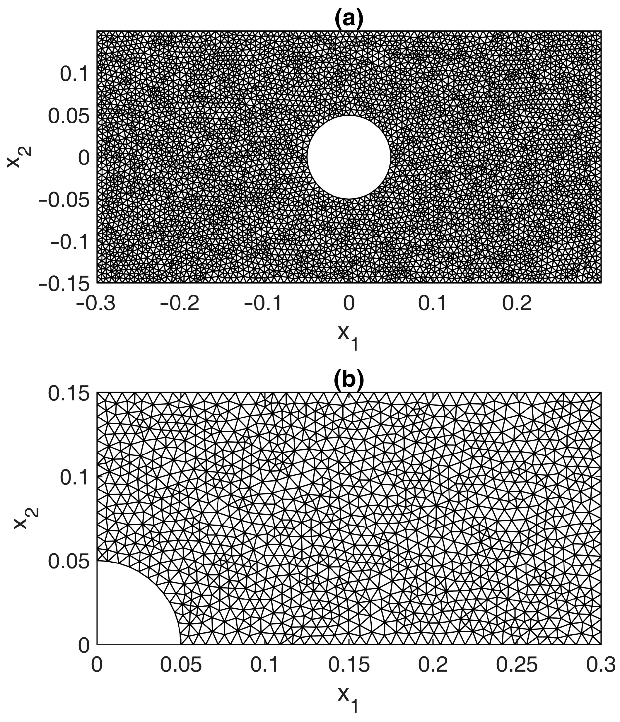
Figure 2 presents the finite element meshes. Their physical densities are comparable. The full Airy–Morley mesh (Figure 2a) contains 5372 nodes and 10,452 triangular elements, corresponding to 6.072 × 10⁴ elements per unit area. It has 21,196 Morley degrees of freedom, of which 20,615 remain independent after the boundary constraints are imposed. The quarter displacement mesh (Figure 2b) contains 1301 nodes and 2480 three-node triangular elements, corresponding to 5.763 × 10⁴ elements per unit area. It has 2602 displacement degrees of freedom and 2552 free unknowns. The displacement-to-Airy mesh-density ratio is 0.949.

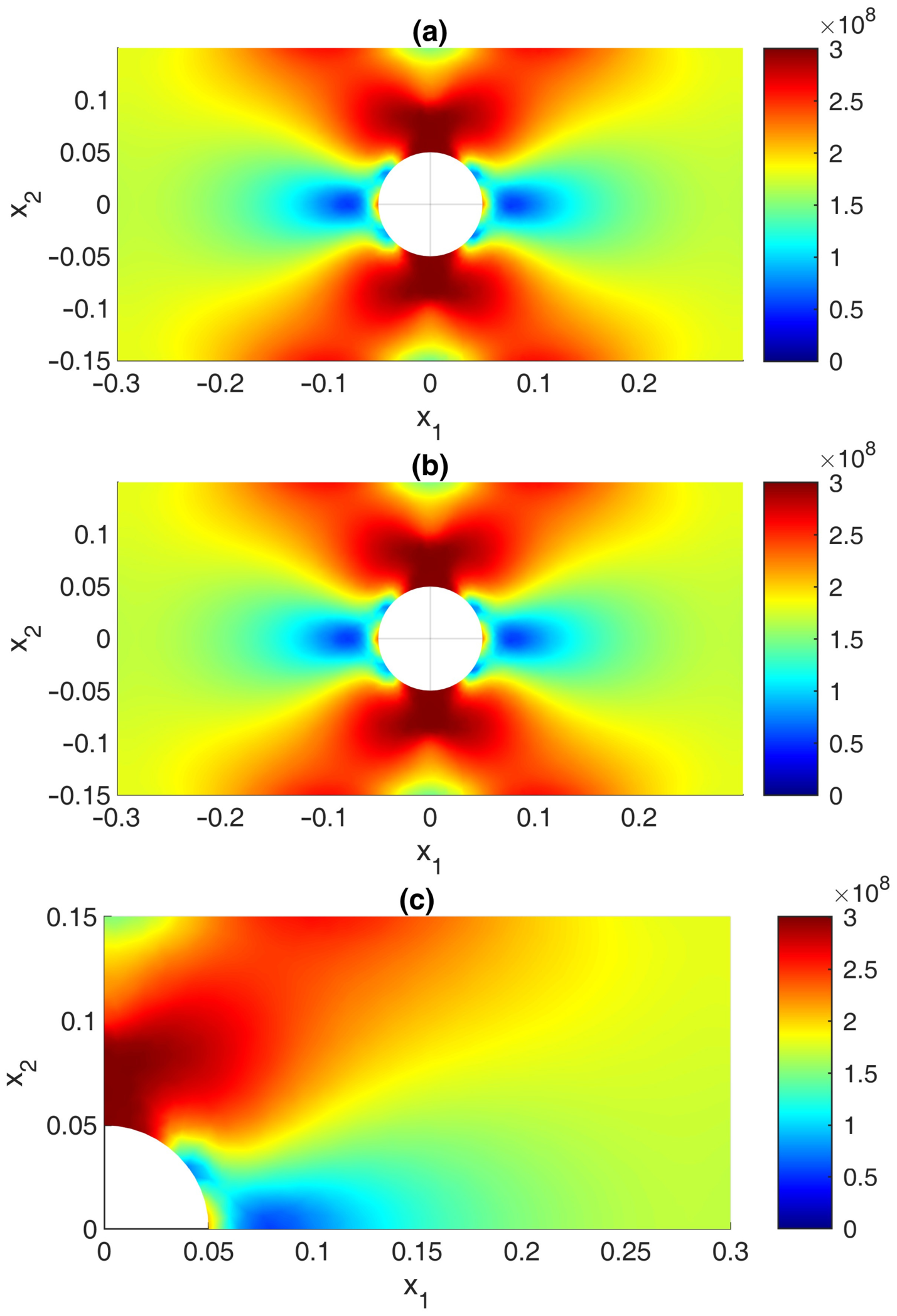
Both discretizations produce element-wise constant stresses. To improve the readability of the contour plots, the element stress components were recovered at mesh nodes by area-weighted averaging and then linearly interpolated within each triangle. The displayed von Mises stress was calculated from these recovered nodal stress components. This recovery procedure was used only for visualization. All maxima, profile errors, plastic-zone measures, residuals, and other numerical quantities were calculated from the original element-wise fields. The plastic strain contours were not smoothed.

6.1. Elastic Verification

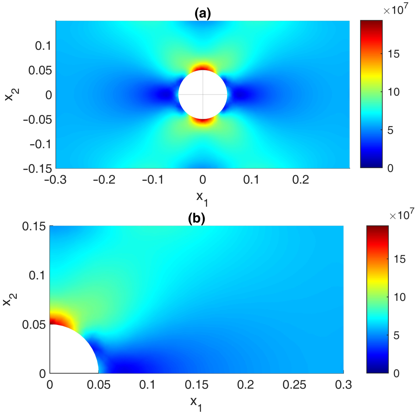
The elastic response is compared at $p=60 \mathrm{MPa}$, before the onset of yielding. Figure 3 shows the recovered von Mises stress fields obtained from the Airy–Morley and displacement formulations. Both models predict the same stress concentration pattern around the hole. The maximum element-wise von Mises stress is 206.951 MPa for the Airy–Morley solution and 208.379 MPa for the displacement solution. The difference between the maxima is approximately 0.69%.

The relative $L^2$ profile differences between the selected element-wise stress profiles are 2.72% for ${\sigma }_{11}$ and 3.90% for the von Mises stress along the horizontal ligament. The corresponding differences are 10.93% for ${\sigma }_{22}$ along the vertical ligament and 10.47% for the circumferential stress near the hole.

The larger differences in ${\sigma }_{22}$ and circumferential stress are associated with their strong local variation near the hole and, in the case of ${\sigma }_{22}$, with relatively small values and changes in sign. The comparison nevertheless confirms that the Airy–Morley formulation reproduces the reference elastic stress field before the plastic constitutive update becomes active.

6.2. Airy Stress Function

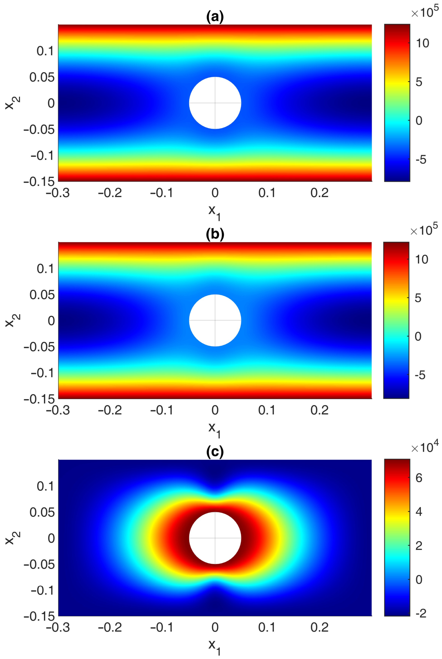
Figure 4a,b compare the elastic and elastoplastic Airy stress functions at the maximum applied traction. Their overall distributions are similar because the external loading dominates both fields. The affine part is removed before comparison because it does not contribute to the stress field. The resulting difference (Figure 4c) is localized around the hole and represents the modification caused by the plastic-strain source term. Although the change in the Airy function is relatively small, its second derivatives produce the observed redistribution of stresses.

6.3. Onset and Development of Plasticity

All three analyses detect the first nonzero plastic strain at $p=90 \mathrm{MPa}$. At the previous load level, $p=84 \mathrm{MPa}$, the maximum equivalent stress is 289.732 MPa in the Airy–Morley solution and 291.730 MPa in the displacement model. Thus, the actual onset of yielding lies between 84 and 90 MPa.

Figure 5 presents the recovered von Mises stress fields at the maximum applied traction. All three models predict the same general redistribution of stress around the hole. After the onset of yielding, the maximum element-wise equivalent stress remains close to the yield stress of 300 MPa, as expected for perfect plasticity.

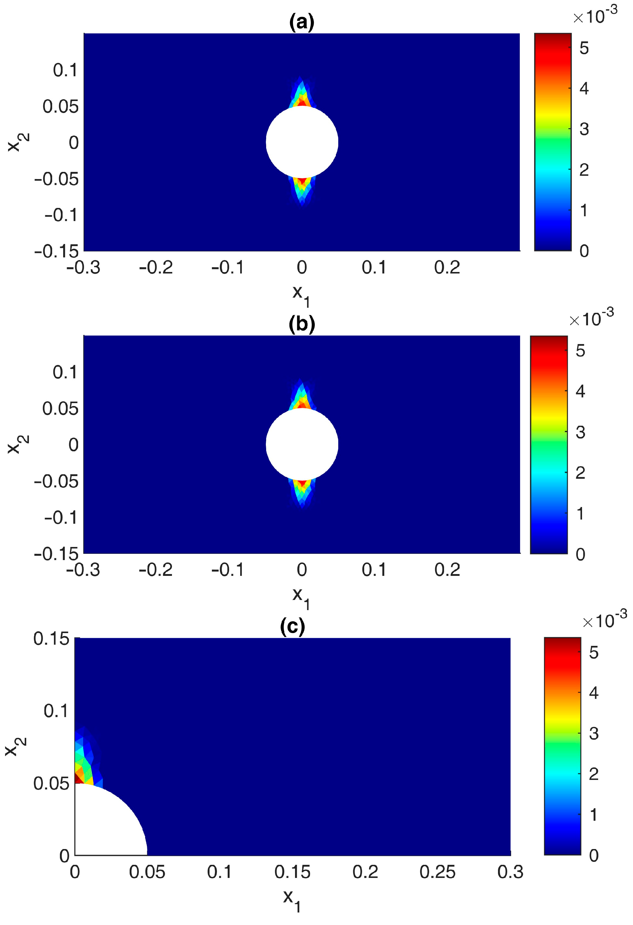
Figure 6 presents the element-wise equivalent plastic strain. In all three solutions, plastic deformation is localized near the upper and lower points of the hole. The positions and general shapes of the plastic zones agree well. To quantify the size of the plastic zone, the plastic area fraction is introduced. For each element, let ${\alpha }_e$ be the accumulated equivalent plastic strain. The plastic area fraction is defined as

$$A_{pl}^{rel}={\displaystyle \frac{{\sum }_{e=1}^{n_{ el}}{A}_{ e} I\left({\alpha }_e>{\alpha }_{tol}\right)}{{\sum }_{e=1}^{n_{ el}}{A}_{ e}}}$$

(55)

Here, $I\left(\cdot \right)$ is the indicator function and ${\alpha }_{tol}$ is a small threshold used to distinguish yielded elements from purely elastic ones. In the present computations, ${\alpha }_{tol}=10^{-9}$. The values reported in

Table 2. Results at $p=180 \mathrm{MPa}.$

Method	Maximum von Mises Stress [MPa]	Maximum Equivalent Plastic Strain	Plastic Area Fraction [%]
Airy–Morley, return-mapping	300.926	4.930 × 10−3	1.805
Airy–Morley, cutting-plane	300.777	4.716 × 10−3	1.805
Displacement FEM	300.000	5.347 × 10−3	1.891

are given as percentages of the analyzed domain area. For the quarter displacement model, the same definition is applied to the quarter domain. By symmetry, this value is directly comparable with the full-domain Airy–Morley result. The final numerical results are summarized in Table 2.

The maximum plastic strain obtained with Airy return-mapping is approximately 7.8% lower than the displacement results. The cutting-plane result is approximately 11.8% lower. In contrast, the predicted plastic area fractions are very close. The difference between the Airy and displacement values is only 0.086 percentage points.

6.4. Influence of the Local Integration Algorithm

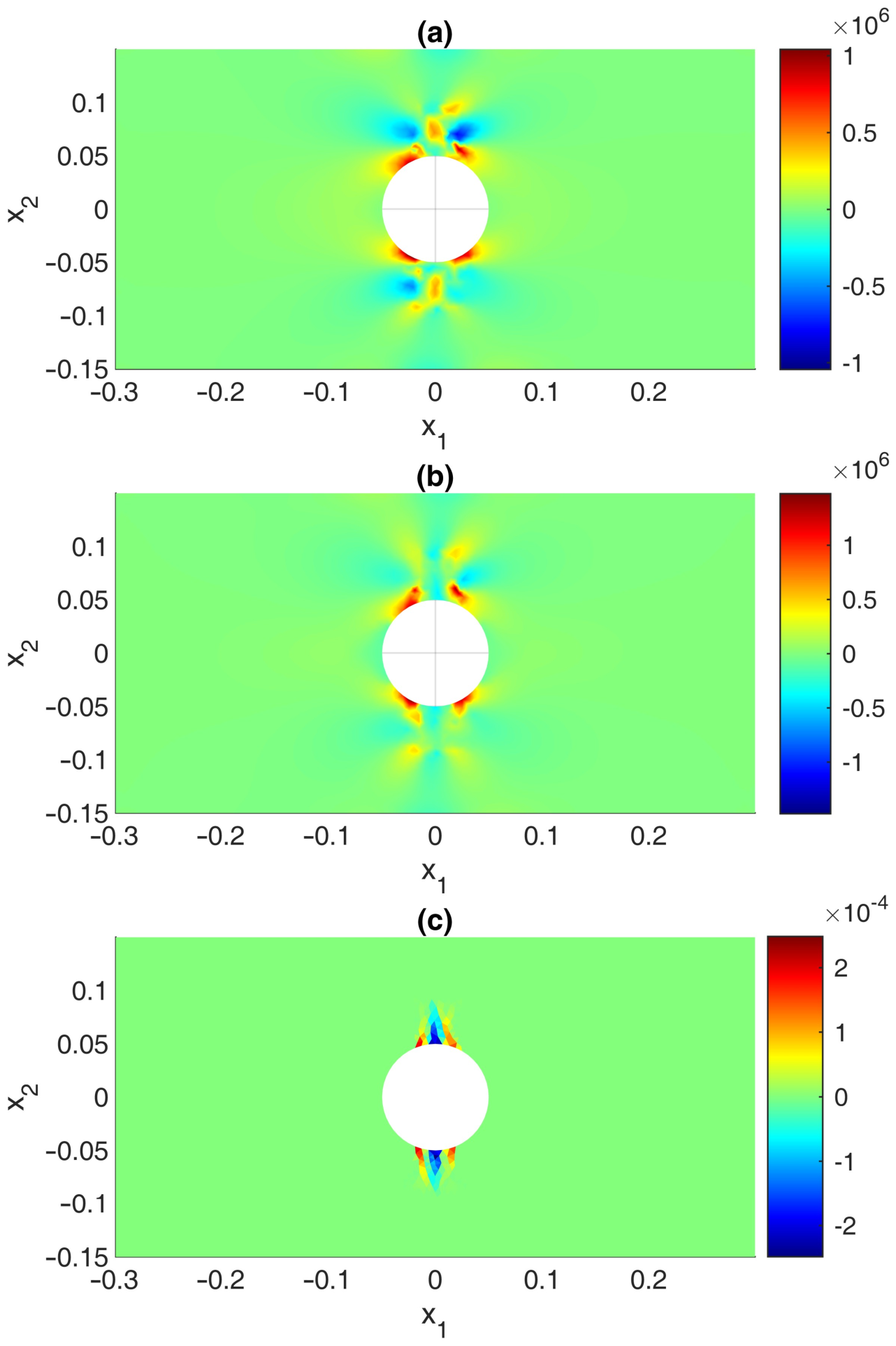
Figure 7 shows the differences between the Airy cutting-plane and return-mapping solutions. The displayed stress differences were obtained from the recovered nodal fields, while the plastic-strain difference remains constant element-wise. The differences are localized near the hole and are small compared with the magnitudes of the corresponding fields.

The differences between the two Airy–Morley integration algorithms are quantified by the relative element-wise $L^2$ measure. For an element-wise scalar quantity $q_e$, it is defined as

$$E_{L^{ 2}}\left(q\right)={\left[{\displaystyle \frac{{\sum }_{e=1}^{n_{ el}}{A}_{ e}{\left(q_e^{\mathrm{CP}}-q_e^{\mathrm{RM}}\right)}^2}{{\sum }_{e=1}^{n_{ el}}{A}_{ e}{\left(q_e^{\mathrm{RM}}\right)}^2}}\right]}^{ {\displaystyle \frac{1}{2}}}$$

(56)

The relative element-wise $L^2$ differences are: 0.052% for ${\sigma }_{11}$; 1.33% for ${\sigma }_{22}$; 0.56% for ${\sigma }_{12}$; 0.052% for the von Mises stress; and 4.12% for the equivalent plastic strain.

The accumulated plastic strain is more sensitive to the integration procedure because small differences generated during successive load increments are retained in this history variable. Nevertheless, both algorithms predict almost identical stress fields, the same first yielding load, and the same final plastic area fraction.

The Airy return-mapping analysis required 9.01 s, whereas the cutting-plane analysis required 4.29 s. The cutting-plane procedure is therefore faster in the present implementation.

6.5. Stress Profiles and Loading Histories

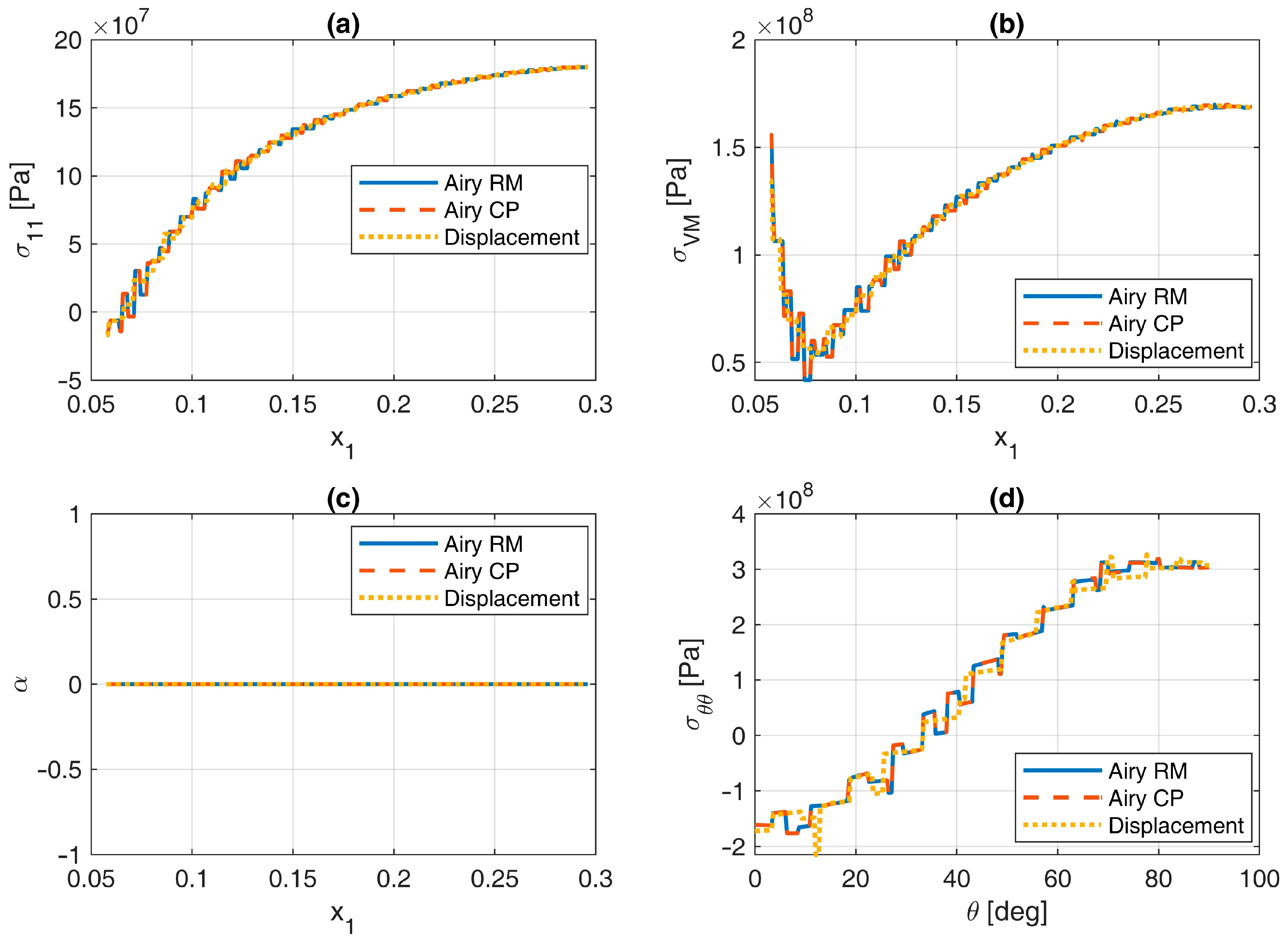
Figure 8 compares selected element-wise profiles at $p=180 \mathrm{MPa}$. No nodal recovery or contour smoothing was used for these curves. The step-like variations follow directly from the element-wise constant stress approximation. The profile differences were quantified using the relative $L^2$ measure defined in Equation (56), with the element-area sums replaced by one-dimensional numerical integration along the corresponding sampling path.

The relative $L^2$ profile differences between Airy return-mapping and the displacement solution are 2.72% for ${\sigma }_{11}$ and 4.32% for the von Mises stress along the horizontal ligament. The corresponding differences are 15.43% for ${\sigma }_{22}$ along the vertical ligament and 9.91% for the circumferential stress near the hole. The larger relative difference in ${\sigma }_{22}$ is partly caused by its relatively small magnitude and changes in sign. The circumferential stress profiles show similar angular variation and comparable peak values in all three models. The equivalent plastic strain along the horizontal ligament remains zero. This agrees with Figure 6, which shows that the plastic zones develop above and below the hole rather than along the horizontal axis.

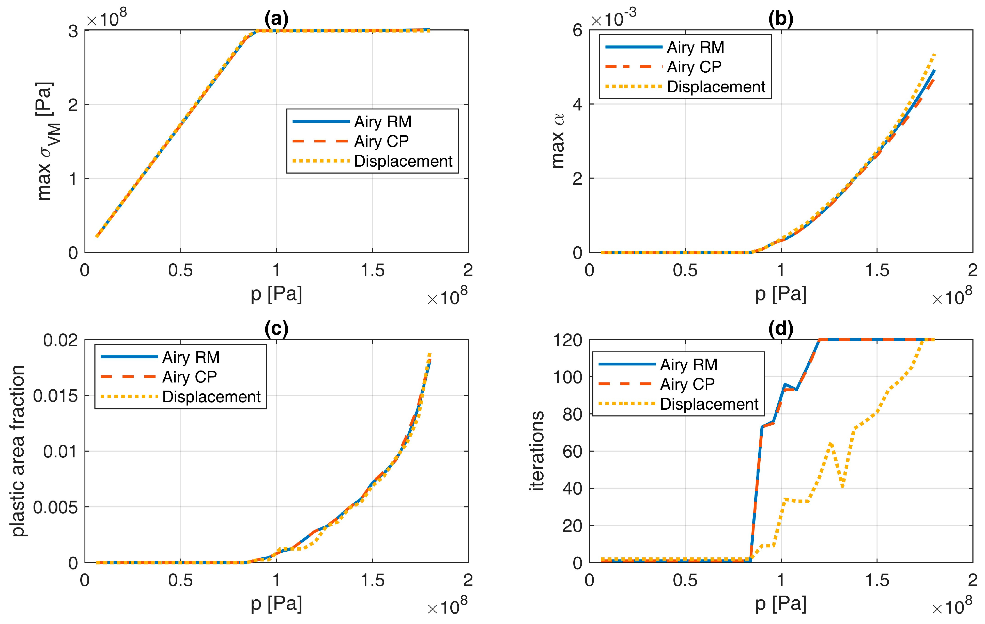
Figure 9 presents the loading histories. Before yielding, the maximum von Mises stress increases linearly with the applied traction. After yielding begins, it remains close to 300 MPa, while the maximum equivalent plastic strain and plastic area fraction increase monotonically. The three formulations predict similar transitions from elastic to elastoplastic behavior.

The Airy analyses reach the imposed limit of 120 global iterations at the higher load levels. At $p=180 \mathrm{MPa}$, the maximum positive yield-function residual is 0.926 MPa for return-mapping and 0.777 MPa for cutting-plane. These values correspond to approximately 0.31% and 0.26% of the yield stress. The displacement model reaches the iteration limit only in the final two load steps. Its normalized equilibrium residual is 1.59 × 10⁻⁵ at 174 MPa and 5.10 × 10⁻⁵ at 180 MPa. The local yield-function violation in the final displacement solution is negligible.

Reaching the iteration limit indicates that the present fixed-point coupling is less robust than the solution procedure used in the displacement model at high elastoplastic load levels. Its robustness in more strongly plastic problems therefore requires further study.

6.6. Computational Cost

The full-domain Airy–Morley model contains 20,615 independent unknowns, whereas the quarter-domain displacement model contains 2552 free unknowns. The total times were 9.01 s for the Airy–Morley formulation with return-mapping integration, 4.29 s with cutting-plane integration and 11.07 s for the displacement formulation with return-mapping integration. Taking the quarter-domain area as one unit, a simple area normalization gives 2.25 and 1.07 s for the two Airy–Morley analyses, respectively, compared with 11.07 s for the displacement analysis. These normalized values are descriptive only and are not estimates of actual quarter-domain Airy–Morley runtimes, because computational cost does not scale linearly with area or number of unknowns. The results therefore support the term “computationally competitive” only for the present benchmark.

The Airy–Morley formulation provides stresses directly and satisfies equilibrium inside each element. However, it does not necessarily reduce computational cost or improve stress accuracy, and the reported timings are specific to this benchmark. Traction boundary conditions are convenient, while prescribed displacements and complex boundaries are less direct. The method is mainly limited to small-strain, two-dimensional plane-stress problems. More complex materials, contact, body force and three-dimensional problems require further development.

6.7. Mesh Sensitivity

A three-level h-refinement study was performed. The standard Morley element has fixed quadratic interpolation. Therefore, p-refinement was not considered. The same physical sampling paths and the same refined displacement–FEM comparison solution were used for all meshes. In

Table 3. Mesh sensitivity results.

$\mathit{p}$	Mesh	Elements	${\mathit{h}}_{\mathit{h}\mathit{o}\mathit{l}\mathit{e}}$	Rel. ${\mathit{L}}^2$ Diff. ${\mathit{\sigma }}_{11}$	Rel. ${\mathit{L}}^2$ Diff. ${\mathit{\sigma }}_{\mathit{e}\mathit{q}}$	Rel. ${\mathit{L}}^2$ Diff. ${\mathit{\sigma }}_{22}$	Rel. ${\mathit{L}}^2$ diff. ${\mathit{\sigma }}_{\mathit{\theta }\mathit{\theta }}$	Max. Equiv. Plastic Strain	Plastic Area Fraction
[MPa]			[mm]	[%]	[%]	[%]	[%]	[-]	[%]
60	Coarse	5126	9.802	3.60	5.19	15.16	16.77	–	–
60	Medium	10,408	6.540	2.37	3.15	12.70	12.58	–	–
60	Fine	20,468	4.907	1.63	2.42	7.41	8.69	–	–
180	Coarse	5126	9.802	3.65	5.58	19.95	16.68	4.816 × 10−3	1.870
180	Medium	10,408	6.540	2.45	3.41	15.07	11.00	4.977 × 10−3	1.788
180	Fine	20,468	4.907	1.70	2.61	12.63	8.18	4.904 × 10−3	1.679

, $h_{hole}$ denotes the mean edge length on the hole boundary, while the stress differences are relative $L^2$ profile measures calculated as described in Section 6.5. All stress-profile differences decrease with refinement at both load levels, although ${\sigma }_{22}$ remains the most mesh-sensitive component. Between the medium and fine meshes, the maximum equivalent plastic strain changes by 1.5% and the plastic area fraction changes by 0.109 percentage points. At 180 MPa, the medium and fine Airy–Morley analyses reached the iteration limit, with positive yield residuals below 0.12% of ${\sigma }_Y$. Therefore, the elastoplastic results are interpreted as mesh-sensitivity indicators rather than a formal asymptotic convergence study.

7. Conclusions

This paper presented the Airy–Morley formulation for two-dimensional elastoplastic plane-stress problems with holes. The non-homogeneous biharmonic equation was discretized by the nonconforming Morley finite element. Plastic strains entered the formulation through the weak-form right-hand side, which avoided the direct evaluation of their second derivatives.

The original contribution lies in the direct combination of the Airy stress function, the Morley finite element, and an incremental elastoplastic material update. The local cutting-plane and return-mapping procedures are standard. The new aspect is their coupling with a global stress-function-based finite element formulation. Unlike classical displacement FEM, the Airy–Morley formulation uses a scalar stress function as the global unknown, and the stresses are recovered directly from its second derivatives. Consequently, the differential equilibrium equations are satisfied inside each element through the Airy representation, while interelement coupling is provided by the nonconforming Morley weak formulation.

The method was implemented in MATLAB using custom routines for finite element assembly, boundary constraints, constitutive integration, and post-processing. The proposed formulation was compared with a classical displacement-based elastoplastic model using meshes of comparable physical density.

For the plate with a circular hole, both Airy–Morley variants reproduced the elastic stress concentration, the onset of yielding, the redistribution of stresses, and the growth of the plastic zone. All models detected the first plastic strains within the same load increment. At the maximum load, the predicted von Mises stress remained close to the yield stress, while the maximum equivalent plastic strain and the plastic area fraction agreed reasonably well with the displacement-based reference solution. However, the validation is limited to one symmetric perforated plate under uniform tension. Therefore, the results demonstrate the feasibility of the formulation rather than its general applicability.

The cutting-plane and return-mapping Airy solutions were almost identical in terms of stresses. Larger differences occurred only in the accumulated plastic strain, which is more sensitive to small errors from previous load increments. In the present implementation, the cutting-plane algorithm was also faster than return-mapping. These results indicate that both local integration procedures can be used with the proposed global formulation.

The main limitations of the Airy–Morley formulation are its restriction to two-dimensional plane stress, homogeneous isotropic materials, small strains, and relatively simple external boundaries. The Morley approximation also produces element-wise constant stresses and plastic strains. Nodal stress recovery improves the presentation of contour plots, but all quantitative results should remain based on the original element fields. Moreover, the current global elastoplastic coupling uses a fixed-point iteration, which may require many iterations at high plastic load levels.

The present study does not attempt to determine the limit load directly. This could be addressed by a separate rigid-plastic limit analysis: for example, using conic programming formulations [27,28].

Further work should focus on a more efficient global solution strategy, including Newton or quasi-Newton coupling and a consistent algorithmic tangent. More generally, recent structure-preserving Galerkin approaches for constrained variational problems suggest that inequality-constrained nonlinear formulations may benefit from dedicated algebraic treatment beyond classical fixed-point iterations [29]. A rigorous asymptotic convergence analysis, error estimation and adaptive refinement near plastic fronts remain topics for future work. Additional benchmarks should include multiple holes, nonuniform tractions, different hole arrangements, and geometries with stronger stress gradients. An extension to more general nonlinear settings, including contact or topology optimization with internal contact, would require additional modeling ingredients and is outside the scope of the present study [30]. A theoretical analysis of consistency, stability, and convergence of the elastoplastic Airy–Morley formulation would provide an important mathematical foundation for the method.

References

- Persson, B.N.J. Surface Roughness-Induced Stress Concentration. Tribol. Lett. 2023, 71, 66. [Google Scholar] [CrossRef]
- Pilkey, W.; Pilkey, D. Peterson’s Stress Concentration Factors, 3rd ed.; John Wiley & Sons: Hoboken, NJ, USA, 2008. [Google Scholar]
- Belytschko, T.; Liu, W.K.; Moran, B. Nonlinear Finite Elements for Continua and Structures, 2nd ed.; John Wiley & Sons: Chichester, UK, 2014. [Google Scholar]
- Aycock, K.I.; Rebelo, N.; Craven, B.A. Method of Manufactured Solutions Code Verification of Elastostatic Solid Mechanics Problems in a Commercial Finite Element Solver. Comput. Struct. 2020, 229, 106175. [Google Scholar] [CrossRef]
- Bathe, K.J. Finite Element Procedures in Engineering Analysis; Prentice Hall: Englewood Cliffs, NJ, USA, 1996. [Google Scholar]
- Pian, T.H.H.; Sumihara, K. Rational Approach for Assumed Stress Finite Elements. Int. J. Numer. Methods Eng. 1984, 20, 1685–1695. [Google Scholar] [CrossRef]
- Arnold, D.; Falk, R.; Winther, R. Mixed Finite Element Methods for Linear Elasticity with Weakly Imposed Symmetry. Math. Comput. 2007, 76, 1699–1723. [Google Scholar] [CrossRef]
- Airy, G.B. On the Strains in the Interior of Beams. Philos. Trans. R. Soc. Lond. 1863, 153, 49–80. [Google Scholar] [CrossRef]
- Morley, L.S.D. A Variational Method of Solution for Problems in Plane Elasticity. IMA J. Appl. Math. 1965, 1, 76–100. [Google Scholar] [CrossRef]
- Morley, L.S.D. The Triangular Equilibrium Element in the Solution of Plate Bending Problems. Aeronaut. Q. 1968, 19, 149–169. [Google Scholar] [CrossRef]
- Engel, G.; Garikipati, K.; Hughes, T.J.R.; Larson, M.G.; Mazzei, L.; Taylor, R.L. Continuous/Discontinuous Finite Element Approximations of Fourth-Order Elliptic Problems in Structural and Continuum Mechanics with Applications to Thin Beams and Plates, and Strain Gradient Elasticity. Comput. Methods Appl. Mech. Eng. 2002, 191, 3669–3750. [Google Scholar] [CrossRef]
- Brenner, S.C.; Sung, L.-Y. C Interior Penalty Methods for Fourth Order Elliptic Boundary Value Problems on Polygonal Domains. J. Sci. Comput. 2005, 22, 83–118. [Google Scholar] [CrossRef]
- Magome, N.; Morita, N.; Kaneko, S.; Mitsume, N. Higher-Continuity s-Version of Finite Element Method with B-Spline Functions. J. Comput. Phys. 2024, 497, 112593. [Google Scholar] [CrossRef]
- Brenner, S.C.; Scott, L.R. The Mathematical Theory of Finite Element Methods, 3rd ed.; Texts in Applied Mathematics; Springer: New York, NY, USA, 2008; Volume 15. [Google Scholar]
- Křížek, M. Conforming Equilibrium Finite Element Methods for Some Elliptic Plane Problems. RAIRO. Anal. Numér. 1983, 17, 35–65. [Google Scholar] [CrossRef]
- Vallabhan, C.V.G.; Azene, M. A Finite Element Model for Plane Elasticity Problems Using the Complementary Energy Theorem. Int. J. Numer. Methods Eng. 1982, 18, 291–309. [Google Scholar] [CrossRef]
- Falk, R.S.; Morley, M.E. Equivalence of Finite Element Methods for Problems in Elasticity. SIAM J. Numer. Anal. 1990, 27, 1486–1505. [Google Scholar] [CrossRef]
- Srinivasa, A.R.; Srinivasa, S.M. Inelasticity of Materials: An Engineering Approach and A Practical Guide; Series on Advances in Mathematics for Applied Sciences; World Scientific Publishing Company: Singapore, 2009; Volume 80. [Google Scholar]
- Strang, G.; Fix, G. An Analysis of the Finite Element Method; Prentice-Hall: Englewood Cliffs, NJ, USA, 1973. [Google Scholar]
- Ciarlet, P.G. The Finite Element Method for Elliptic Problems; North-Holland: Amsterdam, The Netherlands, 1978. [Google Scholar]
- Simo, J.C.; Taylor, R.L. Consistent Tangent Operators for Rate-Independent Elastoplasticity. Comput. Methods Appl. Mech. Eng. 1985, 48, 101–118. [Google Scholar] [CrossRef]
- Ortiz, M.; Simo, J.C. An Analysis of a New Class of Integration Algorithms for Elastoplastic Constitutive Relations. Int. J. Numer. Methods Eng. 1986, 23, 353–366. [Google Scholar] [CrossRef]
- Simo, J.C.; Hughes, T.J.R. Computational Inelasticity; Interdisciplinary Applied Mathematics; Springer: New York, NY, USA, 1998; Volume 7. [Google Scholar]
- de Souza Neto, E.A.; Perić, D.; Owen, D.R.J. Computational Methods for Plasticity: Theory and Applications; John Wiley & Sons, Ltd.: Chichester, UK, 2008. [Google Scholar]
- Hughes, T.J.R. The Finite Element Method: Linear Static and Dynamic Finite Element Analysis; Prentice-Hall: Englewood Cliffs, NJ, USA, 1987. [Google Scholar]
- Zienkiewicz, O.C.; Taylor, R.L.; Zhu, J.Z. The Finite Element Method: Its Basis and Fundamentals, 7th ed.; Butterworth-Heinemann: Oxford, UK, 2013. [Google Scholar]
- Makrodimopoulos, A.; Martin, C.M. Lower Bound Limit Analysis of Cohesive-frictional Materials Using Second-order Cone Programming. Int. J. Numer. Methods Eng. 2006, 66, 603–634. [Google Scholar] [CrossRef]
- Zbiciak, A.; Kasprzak, A.; Józefiak, K. Conic Programming Approach to Limit Analysis of Plane Rigid-Plastic Problems. Appl. Sci. 2025, 15, 10729. [Google Scholar] [CrossRef]
- Keith, B.; Surowiec, T.M. Proximal Galerkin: A Structure-Preserving Finite Element Method for Pointwise Bound Constraints. Found. Comput. Math. 2026, 26, 385–481. [Google Scholar] [CrossRef]
- Frederiksen, A.H.; Sigmund, O.; Poulios, K. Topology Optimization of Self-Contacting Structures. Comput. Mech. 2024, 73, 967–981. [Google Scholar] [CrossRef]