Article

High-Order Reliability Analysis of Nonlinear Steel Frames Using SVM-Reconstructed Limit State Function


1
College of Civil Engineering and Geomatics, Guilin University of Technology at Nanning, Nanning 530001, China
2
China Construction Eighth Engineering Division Corp., Ltd., Shanghai 200120, China
*
Author to whom correspondence should be addressed.
Appl. Sci. 2026, 16(15), 7699; https://doi.org/10.3390/app16157699
Submission received: 2 July 2026 / Revised: 24 July 2026 / Accepted: 28 July 2026 / Published: 3 August 2026
(This article belongs to the Section Civil Engineering)

Abstract

In complex nonlinear steel frames, the limit-state function is typically nonlinear and implicit, which hinders the direct application of traditional first- and second-order reliability methods (FORM/SORM). A reliability analysis approach for steel frames was developed by reconstructing the limit state function using a support vector machine (SVM). Finite-element response samples were employed to construct an explicit SVM surrogate model of the limit state function. The particle swarm optimization (PSO) is adopted to globally optimize the model hyperparameters, thereby enhancing the predictive accuracy and stability of the reconstructed limit-state function. The reconstructed limit-state function was subsequently incorporated into the FORM and SORM frameworks to enable the efficient evaluation of failure probabilities and reliability indices for steel frames. The proposed approach is validated through multiple benchmark examples, including explicit nonlinear limit-state functions and multistory multispan rigid frame structures. The results indicate that the SVM-reconstructed limit-state function accurately captures the non-linear characteristics of the structural responses. The corresponding reliability estimates were in good agreement with the Monte Carlo simulation (MCS) results and previously reported findings. Compared with FORM, SORM significantly improves the accuracy of reliability and failure probability estimation, with the Tvedt formulation demonstrating the highest level of consistency.

1. Introduction

Structural reliability analysis provides a theoretical foundation for evaluating structural safety under uncertainty. Its primary objective is to efficiently estimate the probability integral over the failure domain defined by the limit-state function [1,2]. The first-order reliability method (FORM) [3,4] and second-order reliability method (SORM) [5,6] have been widely employed because of their high computational efficiency and practical applicability in engineering problems. Both approaches generally require an explicit analytical representation of the limit-state function and its differentiability at the most probable failure point (MPP). Reliability assessment is then performed by approximating the limit-state function locally around the MPP using first- or second-order expansions [7].
However, in many practical engineering applications, the limit-state function is implicitly defined through nonlinear finite element simulations or other complex numerical models, making the direct application of FORM and SORM highly challenging [8]. In such cases, the required gradients and curvatures of the limit-state function must typically be obtained through repeated numerical analyses, which can substantially increase the computational costs and introduce additional uncertainties in accuracy control. These limitations are particularly significant for reliability problems involving strong nonlinearities, high-dimensional random variables, or extremely small failure probabilities, where the efficiency and robustness of conventional reliability methods may be considerably compromised.
For engineering problems involving implicit and nonlinear limit-state functions, surrogate modeling techniques have been increasingly adopted to construct explicit approximation models that capture the input-output relationships of finite element simulations or other complex numerical analyses [9]. By replacing computationally intensive numerical models with efficient approximations, surrogate-based methods can significantly reduce the computational cost of reliability assessment. Representative surrogate models include the response surface method (RSM) [10,11], polynomial chaos expansion (PCE) [12], artificial neural networks (ANN) [13,14], and support vector machine (SVM) [15,16,17]. Among these approaches, the SVM-based reconstruction of the limit-state function has demonstrated remarkable potential for structural reliability analysis owing to its capability in dealing with nonlinear and implicitly defined structural responses [18]. Moreover, the reconstructed limit-state function can be conveniently coupled with MCS and advanced reliability methods to improve computational efficiency. Nevertheless, the predictive accuracy and generalization capability of the SVM model are strongly influenced by the selection of kernel function parameters and penalty coefficients. Improper parameter settings may lead to inadequate approximation accuracy, poor generalization performance, or numerical instability [19]. To overcome this limitation, intelligent optimization algorithms, including Bayesian optimization (BO) [19,20], particle swarm optimization (PSO) [21,22], and genetic algorithm (GA) [23,24], have been introduced to globally optimize the SVM hyperparameters. By automatically searching for the optimal model parameters, these optimization strategies can further enhance the accuracy, robustness, and reliability of the SVM-based reconstructed limit-state function.
Regarding reliability assessment, most existing studies have mainly focused on coupling SVM-reconstructed limit-state functions with FORM [25], whereas relatively limited attention has been devoted to their integration with higher-order reliability methods, particularly SORM. Because SORM requires an explicit analytical representation of the limit-state function as well as its first- and second-order derivatives, its direct application to nonlinear structural systems described by implicit finite element models remains challenging. Among the various second-order reliability formulations, the Tvedt approximation has been demonstrated to provide improved accuracy in estimating failure probabilities for nonlinear reliability problems [26]. Therefore, integrating an accurately reconstructed SVM surrogate model with SORM provides an effective approach for extending higher-order reliability analysis to engineering problems involving implicit limit-state functions.
Motivated by this research gap, this study did not propose a fundamentally new reliability analysis method. Instead, it develops an integrated computational framework that combines a PSO-optimized SVM surrogate model with established reliability methods, including the FORM and several SORM formulations, with a particular emphasis on the Tvedt approximation. The proposed framework was applied to the reliability analysis of nonlinear rigid-frame structures with an implicit limit-state function. Its accuracy, robustness, and computational efficiency were evaluated through benchmark nonlinear limit-state functions and nonlinear finite-element models. The results demonstrate that the proposed framework can effectively reconstruct the nonlinear limit-state function and provide reliable and efficient reliability estimates for the investigated structural systems while retaining the advantages of conventional higher-order reliability methods.

2. Review of FORM and SORM

2.1. Reliability Assessment

Structural reliability analysis aims to evaluate the probability of structural failure P f , which can be expressed as [1,2,27]:
P f = P G ( X ) 0 = Ω f f X ( X ) d X
where X denotes the vector of basic random variables; G ( X ) is the limit-state function used to determine the structural safety condition; Ω f = X | G ( X ) 0 defines the failure domain in the random variable space, and f X ( X ) is the joint probability density function. In practical engineering applications, the limit-state function is generally implicit and nonlinear because it is typically obtained from finite-element analysis rather than analytical expressions. Therefore, the direct evaluation of the above integral becomes computationally expensive, particularly for large-scale nonlinear structural systems. To overcome this difficulty, approximate reliability methods such as FORM and SORM are widely adopted.

2.2. Nataf Transformation

The FORM and SORM are formulated in a standard normal space [1,2,27,28]. Therefore, the original correlated random variables X i ,   i = 1 ~ n are first transformed into independent standard normal variables V i using Nataf transformation:
V i = Φ 1 ( F X ( X i ) ) ,   i = 1 , 2 , , n
where F X ( ) is the marginal cumulative distribution function and Φ 1 ( ) is the inverse standard normal cumulative distribution function.
For correlated random variables, the correlation matrix is decomposed using the Cholesky decomposition:
ρ V = L L T
and the correlated standard normal variables are transformed into independent standard normal variables through:
U = L 1 V
After the aforementioned Nataf transformation, the limit state function in the original space ( X -space or physical space), G X ( X ) , can be mapped into the standard normal space ( U -space), G U ( U ) . Through this transformation, the random variable X , originally following an arbitrary probability distribution, is standardized into the random variable U [29,30], where FORM and SORM are conveniently implemented.
The accuracy of the Nataf transformation depends on the correct specification of the correlation structure among the basic random variables and may decrease for highly skewed or heavy-tailed distributions. In the present study, the random variables mainly followed normal or lognormal distributions with moderate correlations, making the Nataf transformation suitable. For more complex dependence structures, alternative methods such as the Rosenblatt transformation or copula-based approaches may be adopted.

2.3. First-Order Reliability Method (FORM)

The FORM approximates the limit-state function using a first-order Taylor expansion at the MPP, as follows:
G X ( X ) = G U ( U ) G ( u * ) + G T ( u * ) ( U u * )
where u * denotes the MPP in the independent standard normal space ( U -space). G ( u * ) represents the gradient vector of the limit state function evaluated at the MPP. The gradient vector is expressed as follows:
G = G X x x u
The reliability index is defined as the minimum distance from the origin to the limit-state surface [31]:
β = u * = u * T u *
and the corresponding failure probability is
P f     F O R M = Φ ( β )
where Φ ( ) denotes the cumulative distribution function of the standard normal distribution.
In the FORM, the MPP is commonly determined using the HL-RF algorithm. Because the HL-RF algorithm is well established, its detailed iterative equations are omitted for brevity and can be found in ref. [32].

2.4. Second-Order Reliability Method (SORM)

Unlike FORM, SORM incorporates the local curvature of the limit-state surface through a second-order approximation around the MPP ( U -space),
G U ( U ) G ( u * ) + G T ( u * ) ( U u * ) + 1 2 ( U u * ) T H U ( u * ) ( U u * )
where H U ( ) is the Hessian matrix, defined as:
H U = x u T 2 G X x 2 x u + diag ( G x 2 x u 2 )
Among the various SORM formulations, the Breitung approximation [33] expresses the failure probability as
P f ,   S O R M ( B r e i t u n g ) = Φ ( β ) i = 1 n 1 1 1 + β κ i
β S O R M ( B r e i t u n g ) = Φ 1 P f ,   S O R M ( B r e i t u n g )
where κ i denotes the principal curvature of the limit-state surface calculated from the Hessian matrix H U ( ) at the MPP. The detailed computation of κ i can be found in ref. [33].
To improve the accuracy of SORM for highly nonlinear limit-state surfaces, Tvedt [26] proposed a more general second-order approximation. The corresponding failure probability and reliability index were calculated as follows [26]:
P f ,   S O R M ( T v e d t ) = A 1 + A 2 + A 3
A 1 = Φ ( β ) i = 1 n 1 1 1 + β κ i
A 2 = β   Φ ( β ) Φ ( β ) i = 1 n 1 1 1 + β κ i i = 1 n 1 1 1 + ( β + 1 ) κ i
A 3 = β + 1 β   Φ ( β ) Φ ( β ) i = 1 n 1 1 1 + β κ i Real i = 1 n 1 1 1 + ( β + i ) κ i
β S O R M ( T v e d t ) = Φ 1 P f ,   S O R M ( T v e d t )

3. Reliability Calculation Method Based on Support Vector Machine Model

In complex nonlinear steel frames, the coupled effects of material and geometric nonlinearities together with multiple loading conditions generally require nonlinear finite element analysis (FEA) to obtain the structural response. Consequently, the limit state function is implicitly embedded in the numerical model and cannot be directly expressed as an explicit function of the basic random variables. As indicated by Equations (6) and (10), both FORM and SORM require first- and second-order derivatives of the limit-state function. Therefore, conventional reliability methods cannot be directly applied to implicit finite element (FE) models.
Furthermore, nonlinear FEA of steel-frame structures is computationally expensive, resulting in limited training samples. Under small-sample conditions, Zhou et al. [34] and Su et al. [35] demonstrated that gaussian process regression (GPR) and SVM exhibit good generalization capability and stable prediction accuracy. However, the GPR lacks an explicit representation of the reconstructed limit-state function, making derivative evaluation difficult and limiting its direct application with FORM and SORM. In contrast, the explicit limit-state function reconstructed by SVM with a radial basis function (RBF) enables analytical derivative calculation [36,37], which facilitates the evaluation of the first- and second-order derivatives required by FORM and SORM. Therefore, the RBF-SVM was selected and coupled with FORM and SORM for structural reliability analysis in this study.

3.1. SVM-Based Reconstruction of Limit State Function

The SVM is a machine learning model developed based on statistical learning theory and is supported by a well-established theoretical foundation. It has been widely applied to tasks such as pattern recognition, regression analysis, and function approximation. In support vector regression with a linear loss function, the learning problem can be formulated as the following optimization problem [38]:
min 1 2 ω 2 + C i = 1 m ( ξ i + ξ i ) s . t . ( ω x i + b ) y i ε + ξ i y i ( ω x i + b ) ε + ξ i ξ i , ξ i 0
where x i denotes the sample point, x i = [ x i 1 x i 1 x i n ] T   ( i = 1 ,   2 ,   ,   m ) ; y i represents the corresponding response value; ξ i and ξ i are slack variables; C is the penalty parameter; ε is the insensitive loss parameter; ω and b denote the parameters of the decision function. By applying the Karush–Kuhn–Tucker conditions, the above primal optimization problem can be transformed into the following dual problem [39]:
min 1 2 i = 1 m ( α i * α i ) ( α j * α j ) ( x i x j ) + ε i = 1 m ( α i * + α i ) i = 1 m y i ( α i * α i ) s . t . i = 1 m ( α i * α i ) = 0 0 α i , α i * C
For complex practical engineering structures, the relationship between the structural responses and basic random variables is typically a nonlinear regression problem. Therefore, a nonlinear mapping function is employed to map the sample points into a high-dimensional feature space, where linear support vector regression is performed. The corresponding nonlinear optimization problem can be formulated as [39]:
min 1 2 i = 1 m ( α i * α i ) ( α j * α j ) k ( x i x j ) + ε i = 1 m ( α i * + α i ) i = 1 m y i ( α i * α i ) s . t . i = 1 m ( α i * α i ) = 0 0 α i , α i * C
where k ( x i x j ) denotes the inner product of the random variables in the corresponding feature space after mapping the sample points into the high-dimensional feature space, i.e., k ( x i x j ) = φ ( x i ) φ ( x j ) , which is referred to as the kernel function. Since the RBF kernel exhibits favorable statistical performance, the SVM models developed in this study employ the RBF kernel, expressed as [40]:
k ( x x i ) = exp ( γ x x i 2 )
After solving Equation (20), the reconstructed limit-state function based on the SVM model can be obtained as
G ˜ X ( x ) = i = 1 m ( α i * α i ) k ( x x i ) + b
According to Equations (6) and (10), the application of FORM and SORM in reliability analysis requires the first- and second-order derivatives of the limit-state function. Based on Equations (21) and (22), these quantities can be derived as:
G X x j = G ˜ X x j = i = 1 m 2 γ ( α i * α i ) ( x j x j i ) exp ( γ x x i 2 )
2 G X x j x k = 2 G ˜ X x j x k = i = 1 m 4 γ 2 ( α i * α i ) exp ( γ x x i 2 ) ( x j x j i ) ( x k x k i ) , j k i = 1 m 2 γ ( α i * α i ) exp ( γ x x i 2 ) ( 1 + x j x j i 2 ) ( 1 + x k x k i 2 ) , j = k

3.2. Data Normalization

In the reliability analysis of frame-structure responses, random variables, such as the elastic modulus, material yield strength, applied loads, and cross-sectional dimensions, often have heterogeneous physical units and significantly different numerical scales. Directly training an SVM model on the raw samples may therefore reduce both the prediction accuracy and the generalization capability. To alleviate this issue, the random input variables and corresponding response outputs were normalized prior to model training. Specifically,
t i = x i x min x max x min
s i = y i y min y max y min
where t i represents the normalized sample value of the random input variable, and s i denotes the normalized sample value of the output response variable. Here, x min and x max are the minimum and maximum values of the original random input variable samples before normalization, respectively, while y min and y max denote the minimum and maximum values of the original output response samples before normalization, respectively. After normalization, the first- and second-order derivatives of the limit-state function can be obtained using the following relationships:
G ˜ ( x ) x = G ˜ t y max y min x max x min
2 G ˜ X x j x k = 2 G ˜ X t j t k y max y min ( x j , max x j , min ) ( x k , max x k , min )

3.3. Hyperparameter Optimization

From Equations (20) and (21), it can be observed that the limit-state function reconstructed by the SVM model is jointly governed by the parameters C , γ , and ε . The selection of these parameters had a significant impact on the prediction accuracy of the model. Owing to the complex coupling between these parameters, manual trial-and-error approaches are unlikely to identify the optimal parameter combination. Therefore, PSO [21,22,41] is employed in this study to globally optimize these parameters, enabling automatic tuning of the SVM model and improving the accuracy and stability of the reconstructed limit-state function. PSO is a stochastic optimization algorithm inspired by swarm intelligence. By sharing information and performing cooperative searches among particles, it achieves a balance between global exploration and local convergence, making it particularly suitable for nonlinear multiparameter optimization problems.
In the PSO algorithm, the velocity and position update equations for a particle in the d-th dimension at the n-th iteration are given by Equations (29) and (30), respectively [41]:
v i d n + 1 = ω × v i d n + c 1 × r 1 × ( p i d n x i d n ) + c 2 × r 2 × ( p g d n x i d n )
x i d n + 1 = x i d n + v i d n
where v i d and x i d denote the velocity and position of the particle, respectively; ω is the inertia weight; c 1 and c 2 are acceleration coefficients; r 1 and r 2 are random numbers in the range [0, 1]; and p g d represents the historically best position of the particle.

4. Computational Procedure

4.1. Computational Implementation Details

The main computational procedure adopted in this study to enhance the reproducibility and transparency of the proposed framework is summarized as follows:
(1)
Random sample generation: The probability distributions and statistical parameters of all random variables are specified according to the numerical example described in Section 5. Monte Carlo sampling was employed to generate 2000 training samples for the limit-state function reconstruction, while an independent Monte Carlo simulation with 100,000 samples was conducted as the reference solution. A fixed random seed (rng = 42) was used to ensure reproducibility of the generated samples.
(2)
Data preprocessing: All input variables and corresponding limit-state function values were normalized to the interval [0, 1] using min–max normalization. The generated dataset was randomly divided into a training set (70%) and a testing set (30%) using a fixed random seed (rng = 10).
(3)
SVM hyperparameter optimization: An RBF kernel was adopted for the SVM surrogate model. The hyperparameters, including the penalty parameter C , kernel width γ , and insensitive loss parameter ε , were optimized using PSO. The search ranges were as follows: C 0.1 ,   50 , γ 0.1 ,   10 , and ε 0.001 ,   0 . 1 . PSO employed 20 particles with a maximum of 30 iterations. The inertia weight and acceleration coefficients were set as ω = 0.7 , c 1 = 1.5 , and c 2 = 1.5 , respectively. The root mean square error (RMSE) of the testing dataset was adopted as the fitness function.
(4)
Model validation: To evaluate the generalization capability of the proposed surrogate model, 10-fold cross-validation was performed. The prediction performance was assessed using the coefficient of determination (R2) and the root mean square error (RMSE), and the average results over ten folds were used to evaluate the stability and robustness of the reconstructed limit-state function.
(5)
Reliability analysis: The reconstructed limit-state function was subsequently coupled with the FORM and SORM. FORM was solved using the HL-RF iterative algorithm with a convergence tolerance of 10−3 and a maximum of 100 iterations. The obtained design point and reliability index were then employed in Breitung and Tvedt SORM approximations to estimate the structural failure probability. Finally, the MCS results were adopted as a benchmark for evaluating the prediction accuracy of the proposed framework.

4.2. Finite-Element Implementation

To facilitate the reproducibility of the finite-element analyses, the main modeling procedure adopted in this study is summarized as follows.
(1)
Finite-element model: Nonlinear analyses were performed using ANSYS 2022 R1 APDL. All beams and columns were modeled using a three-dimensional BEAM189 element based on the Timoshenko beam theory. The cross-sectional dimensions of the beams and columns were defined based on the corresponding benchmark examples.
(2)
Material model: Steel was modeled using an elastic–plastic constitutive law with a bilinear isotropic hardening model. The elastic modulus and yield strength were treated as random variables according to the statistical properties defined in each numerical example, while Poisson’s ratio was fixed at 0.30.
(3)
Mesh discretization and boundary conditions: Each beam and column member was discretized into 20 beam elements. The four column bases were fully restrained, and all beam-column joints were assumed to be rigidly connected.
(4)
Loading and nonlinear analysis: Concentrated horizontal loads were applied to each floor level, whereas concentrated and uniformly distributed vertical loads were applied to the beams. The geometric nonlinearity was considered by activating the large-displacement option (NLGEOM, ON). The nonlinear equilibrium equations were solved using the Newton-Raphson iterative algorithm in ANSYS.
(5)
Structural response extraction: After convergence, the horizontal displacement of the top-right corner node is extracted as the structural response. The corresponding displacement response was used to construct the limit-state function for the subsequent SVM training and structural reliability analysis.
The same finite-element modeling strategy was adopted for both the five-story and three-story frame examples presented in Section 5.2 and Section 5.3, respectively. Only the corresponding structural geometry, loading conditions, and statistical properties of the random variables are specified according to the respective benchmark problems.
Furthermore, in this study, MCS was performed using 105 independent random samples to obtain the reference reliability results. The limit-state responses were evaluated directly using the original finite element model rather than the SVM surrogate model. According to previous studies [42,43], 105–106 samples are commonly adopted in MCS-based reliability analysis of frame structures. Therefore, 10 5 samples were selected to balance statistical accuracy and computational efficiency. All numerical simulations were performed on a computer equipped with an Intel® Core™ i7-12650H processor (2.30 GHz), 16 GB RAM, and an NVIDIA GeForce RTX 3050 Laptop GPU (4 GB).

4.3. Gradient and Hessian Transformation of the SVM Surrogate

Because the SVM surrogate model and reliability analysis are conducted in different spaces, a transformation procedure is required to ensure consistency of the derivative information. In this study, the SVM model was constructed in normalized space, whereas FORM and SORM analyses were performed in independent standard normal space. Therefore, the first- and second-order derivatives are sequentially transformed from the normalized space to the physical space, and finally to the standard normal space. The procedure is as follows.
(1)
Derivative calculation in the normalized space: The SVM surrogate model was established using normalized samples to reduce the influence of different variable scales. Thus, the variables in Equations (23) and (24) represent normalized variables, and the first- and second-order derivatives of the limit-state function are initially calculated in normalized space using these equations.
(2)
Transformation to the physical space: The derivatives obtained in the normalized space are transformed into the original physical space using Equations (27) and (28), considering the scaling effects introduced by the normalization process.
(3)
Transformation to the standard normal space: Finally, the gradient vector and Hessian matrix required for the FORM and SORM analyses were obtained by applying the transformations defined in Equations (6) and (10), respectively. Through these transformations, the derivative information of the SVM-reconstructed limit state function is consistently mapped from the original physical space to the independent standard normal space. This process ensures seamless integration of the SVM surrogate model with the FORM/SORM framework and enables accurate evaluation of the reliability index and failure probability.

5. Validation Analysis

The selected benchmark examples included explicit nonlinear limit-state functions and nonlinear finite-element-based steel-frame structures. Explicit functions are widely used for reliability analysis because they provide representative nonlinear failure boundaries for evaluating the surrogate model accuracy. The steel frame examples further verify the applicability of the proposed method to practical engineering problems involving implicit limit-state functions, nonlinear structural responses, and computationally expensive finite element analyses. Together, these examples provide complementary validation from both the mathematical and engineering perspectives.

5.1. Example 1: Explicit Nonlinear Limit State Function

This example considers two representative and nonlinear limit-state functions widely reported in the literature [27,44] to compare the computational accuracy of FORM and SORM in reliability analysis.
Function 1 was originally proposed by Tvedt [44] to describe the limit-state behavior associated with the plastic collapse failure mechanism of a single-story, single-bay frame structure. The random variables in this function follow a lognormal distribution. Specifically, the means and standard deviations of x 1 ~ x 4 were 120 and 12, respectively; those of x 5 were 50 and 15; and those of x 6 were 40 and 12.
Function 2, originally proposed by Lee et al. [27], is commonly used as a benchmark for evaluating the applicability of FORM and SORM in problems involving high-dimensional random variables. In this setting, all random variables are mutually independent and follow a standard normal distribution.
F u n c t i o n   1 :   G ( X ) = x 1 + 2 x 2 + 2 x 3 + x 4 5 x 5 5 x 6 x i ~ L N ( 120 ,   12 )   ,   i = 1 ~ 4 ; x 5 ~ L N ( 50 ,   15 )   ; x 6 ~ L N ( 40 ,   12 )
F u n c t i o n   2 :   G ( X ) = x 1 2 x 2 2 x 3 2 x 4 2 + 10 x 1 + 12 x 2 + 12 x 3 + 12 x 4 43   ,   x i ~ N ( 0 ,   1 )   ,   i = 1 ~ 4
For both limit-state functions, 2000 random samples were initially generated and normalized to improve the numerical stability and training efficiency of the SVM model. Subsequently, the PSO algorithm was employed to optimize the key hyperparameters of the SVM. With the optimal hyperparameter configuration obtained, the SVM surrogate model was trained to reconstruct the corresponding limit state functions. The reconstructed limit-state functions were then integrated with FORM and SORM to evaluate the structural reliability, including the failure probability and reliability index.
Figure 1 presents scatter plots comparing the normalized predictions from the SVM-reconstructed limit-state functions with the reference values. The predicted results for both benchmark functions are closely distributed around the 1:1 line, indicating good agreement between the reconstructed and original functions. Furthermore, the prediction performance was quantitatively evaluated using R2, MAE, and RMSE. As summarized in Figure 1, both functions achieve R2 values of approximately 1.0000 with extremely small MAE and RMSE values, demonstrating that the proposed PSO-SVM model can accurately capture nonlinear limit-state relationships and provide reliable surrogate functions for subsequent reliability analysis.
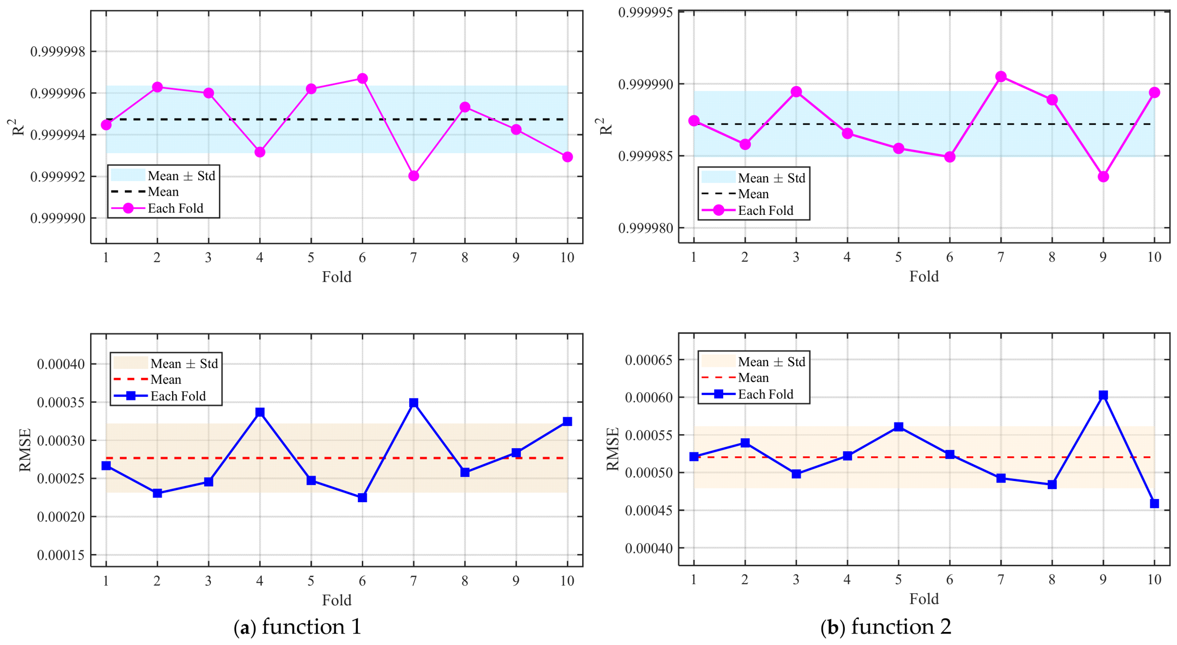
To further examine the generalization capability of the proposed model, a 10-fold cross-validation analysis was conducted, and the results are presented in Figure 2. As shown in Figure 2a,b, the R2 and RMSE values exhibit only slight variations among the ten validation folds for both benchmark functions. The consistently high R2 values and low RMSE values demonstrate that the SVM model maintains stable predictive performance under different data partitions. Therefore, the cross-validation results confirm that the proposed approach has satisfactory generalization capability and does not exhibit significant overfitting when predicting unseen samples.
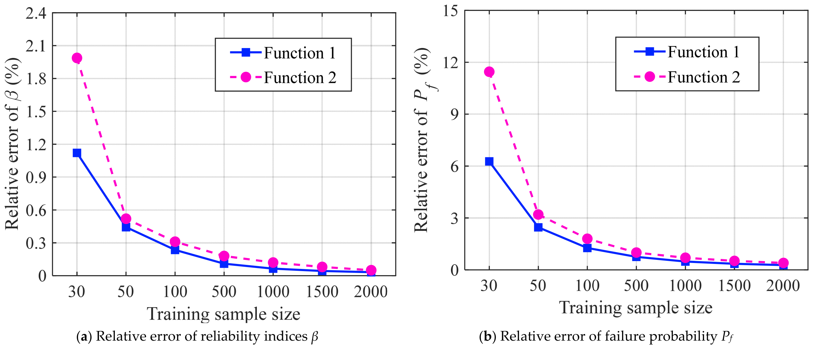
In addition to prediction accuracy and generalization performance, the applicability of the proposed reliability framework under limited training sample conditions was further investigated. A sensitivity analysis was conducted by varying the training sample size, and the relative errors of the reliability index (β) and failure probability (Pf) between SORM (Tvedt) and MCS are presented in Figure 3. The results indicate that the relative errors of both β and Pf gradually decrease with increasing training sample size for the two benchmark functions. When fewer than 500 training samples are employed, relatively larger deviations are observed due to the insufficient information available for accurately reconstructing the nonlinear limit-state surfaces. Furthermore, Function 2 exhibits higher errors under limited sample conditions because its stronger nonlinear characteristics increase the difficulty of capturing the complex response behavior with insufficient training data. As the sample size increases, the reliability predictions become progressively more accurate, and both β and Pf gradually converge and remain stable when the number of training samples exceeds approximately 500–1000.
Following the validation of the SVM reconstruction accuracy, the reliability analysis performance of the proposed framework was further assessed using the two benchmark limit-state functions. The SVM-reconstructed limit-state functions were combined with FORM and SORM to calculate reliability indices and failure probabilities. For the SORM analysis, two widely used approximation schemes, namely, the Breitung and Tvedt formulations, were considered and denoted as SORM (Breitung) and SORM (Tvedt), respectively. The results obtained from MCS were adopted as reference solutions, and additional results reported in previous studies [27,44] were included for comparison.
As summarized in Table 1, the reliability indices and failure probabilities obtained from the proposed framework are in good agreement with the MCS results and published data. The consistent results among the different reliability methods demonstrate that the SVM-reconstructed limit-state functions can accurately preserve the essential nonlinear characteristics of the original functions and provide reliable inputs for subsequent FORM/SORM calculations. For example, for Function 2, the reliability index obtained by SORM (Tvedt) was 2.184, which is very close to the MCS result (2.188) and the reference value reported by Lee et al. [27] (2.188). Similar consistency can be observed in the corresponding failure probabilities.
For completeness and reproducibility, the optimized SVM hyperparameters used in the reconstruction process, including the penalty coefficient C , ε -insensitive loss parameter ε , and kernel parameter γ , are also provided in Table 1.

5.2. Example 2: A Five-Story Three-Bay Rigid Frame Structure

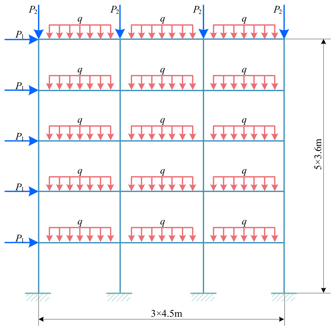
The geometric parameters of the five-story three-bay rigid frame structure, including the story height and span length, are illustrated in Figure 4. The columns adopted the W18 × 86 section, whereas the beams used the W27 × 84 section. The modulus of elasticity E , material yield strength f y , horizontal concentrated load P 1 , the vertical concentrated load P 2 , and uniformly distributed load q are all considered random variables, and their statistical characteristics are summarized in Table 2.
The allowable top displacement of the structure was set as 10 mm. Based on the proposed SVM-based limit-state function reconstruction, the reliability index and failure probability associated with the top displacement are evaluated by coupling the SVM-reconstructed limit-state function with FORM and SORM. In the SORM analysis, both Breitung and Tvedt approximations were employed. The computed results were further compared with those of MCS to verify the accuracy of the proposed method.
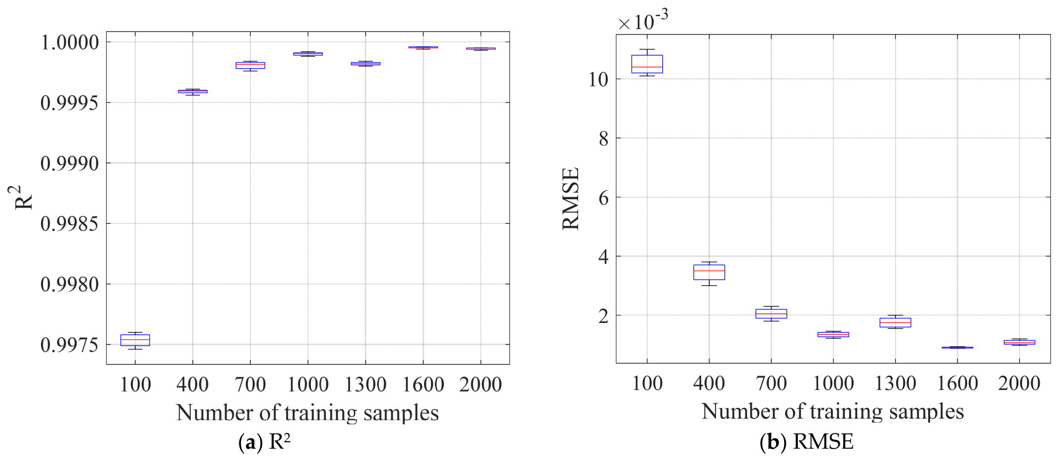
To investigate the influence of training sample size on reliability analysis performance, a sensitivity study was conducted using different numbers of training samples ranging from 100 to 2000. The prediction accuracy of the SVM-reconstructed limit-state function was evaluated in terms of R2 and RMSE. For each training sample size, corresponding boxplots were generated based on six different load variation coefficients (0.05, 0.08, 0.11, 0.14, 0.17, and 0.20), representing different levels of load uncertainty. The results are shown in Figure 5.
As shown in Figure 5a, the R2 values exhibited an increasing trend with an increase in the training sample size. Even with only 100 training samples, the median R2 values remained higher than 0.997, indicating that the proposed SVM model can effectively capture the nonlinear characteristics of the limit-state function under limited data conditions. Moreover, the decreasing dispersion of the boxplots demonstrates an improved prediction stability as more training samples are incorporated.
Figure 5b shows the variation in the RMSE with increasing training sample size. The RMSE decreased significantly when the sample size increased from 100 to approximately 700, after which the improvement became relatively marginal. This indicates that the reconstruction accuracy gradually approached a stable level when sufficient training samples were provided.
Overall, the sensitivity analysis demonstrates that the proposed SVM-based reconstruction strategy maintains a reliable prediction performance under different training sample sizes and load uncertainty levels. The results also indicate that approximately 700–1000 samples are sufficient to achieve a stable approximation accuracy for the investigated structural reliability problem, providing useful guidance for selecting training samples for practical applications.
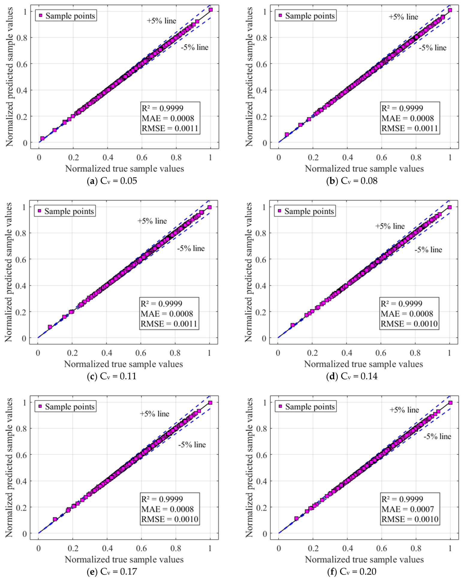
Following the sensitivity analysis of the training sample size, the influence of the load uncertainty on the reconstruction performance was further investigated. Using 2000 training samples, the prediction results of the SVM-reconstructed limit state function under six different load coefficients of variation (Cv = 0.05, 0.08, 0.11, 0.14, 0.17, and 0.20) are presented in Figure 6.
As shown in Figure 6a–f, the normalized predictions exhibit a strong correlation with the reference values, with most data points distributed close to the 1:1 line and located within the ±5% error boundaries. The results indicate that the proposed SVM reconstruction framework maintains a consistent prediction performance under different levels of load uncertainty.
The corresponding statistical indicators are summarized in each subplot. For all the investigated load variation coefficients, the coefficient of R2 remained at approximately 0.9999, whereas the MAE and RMSE values varied within narrow ranges of 0.0007–0.0008 and 0.0010–0.0011, respectively. The small variations in these error metrics demonstrate that changes in load uncertainty have a limited influence on the accuracy of the reconstructed limit-state function. These consistently low prediction errors demonstrate that the SVM-reconstructed limit-state function maintains high numerical accuracy and satisfactory robustness under different levels of load variability.
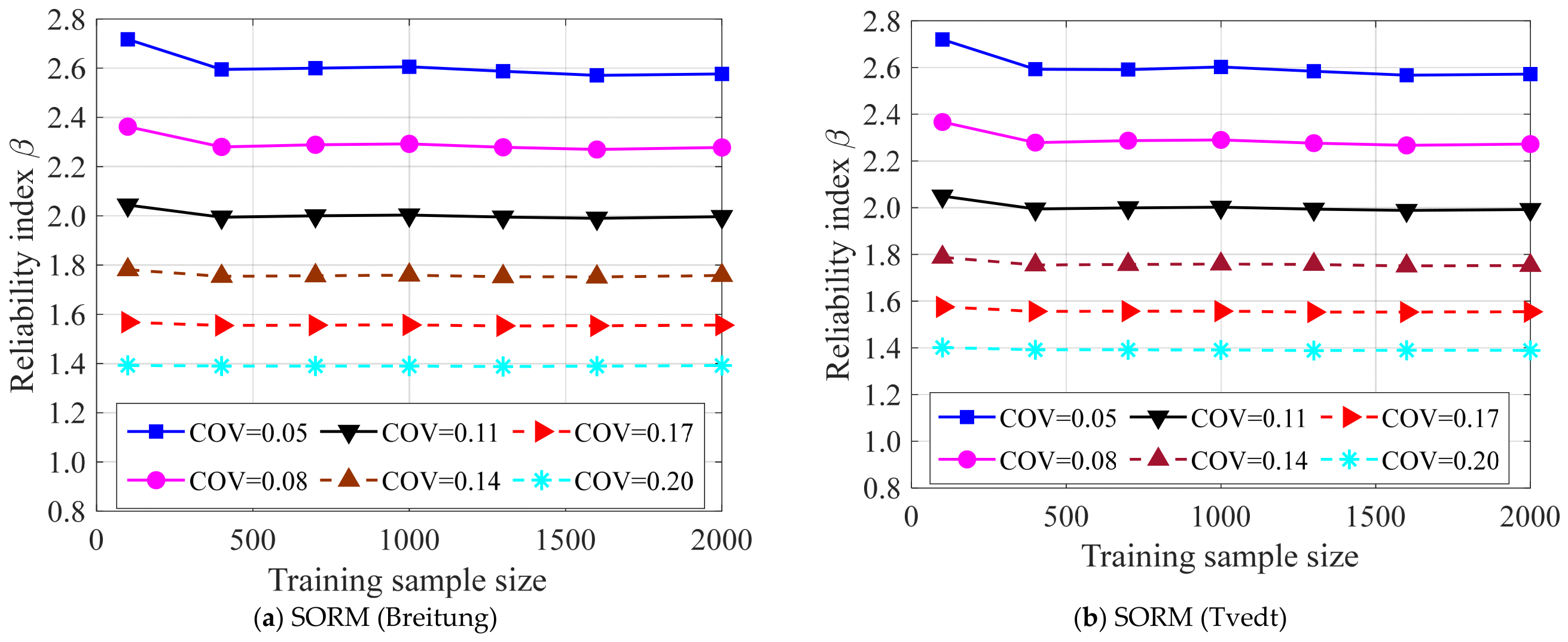
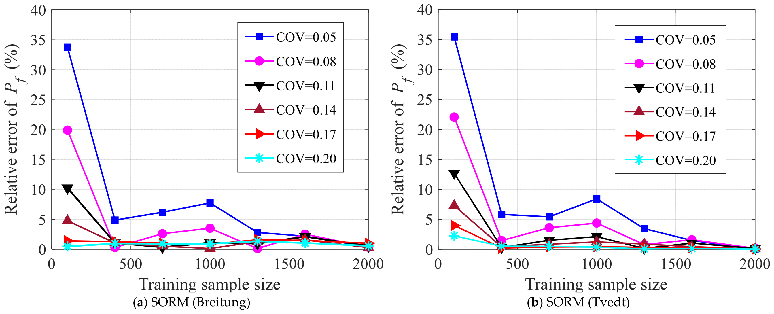
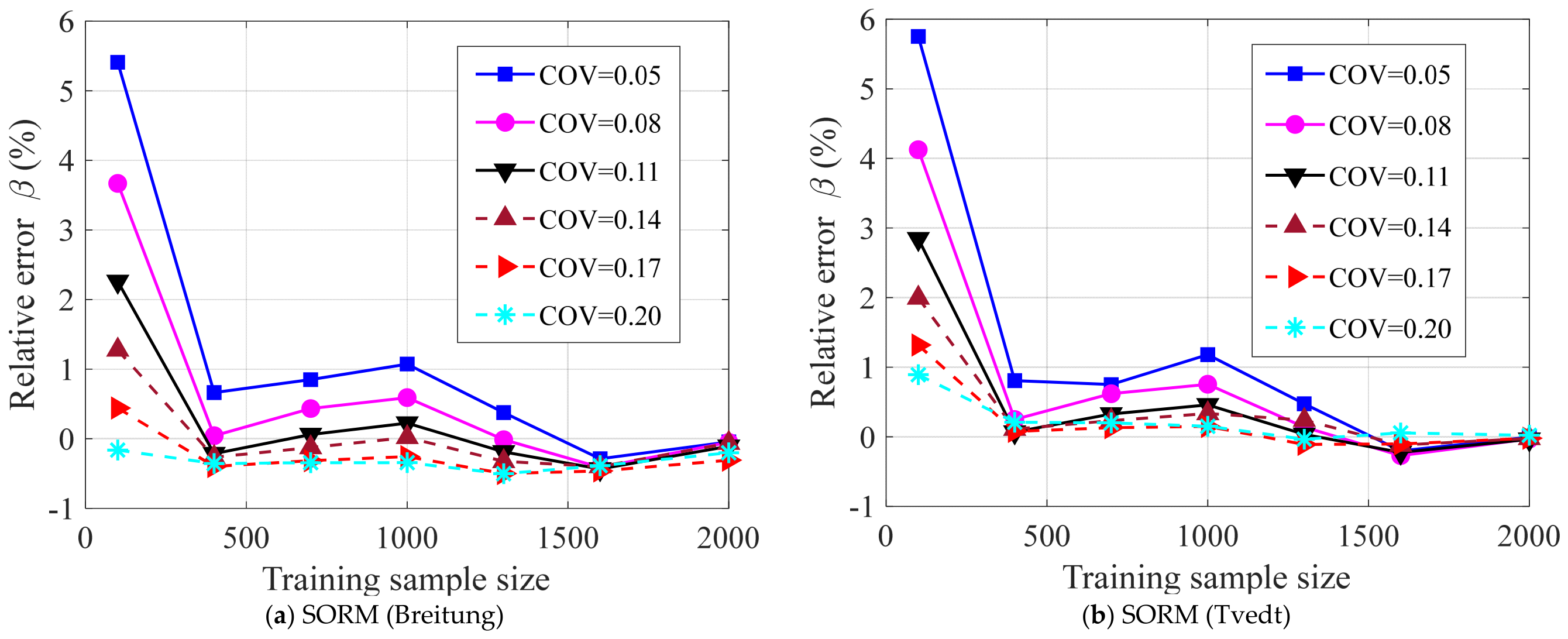
Following the evaluation of reconstruction accuracy, the influence of training sample size on the reliability estimation was further investigated. Based on the SVM-reconstructed limit-state functions, the reliability indices (β) and failure probabilities (Pf) obtained from SORM (Breitung) and SORM (Tvedt), together with their relative errors with respect to the MCS results, are presented in Figure 7, Figure 8 and Figure 9 under different load variation coefficients.
As shown in Figure 7, the β obtained from both SORM formulations exhibit a clear convergence trend with increasing training sample size. When the number of training samples is relatively small, slight fluctuations occur due to the insufficient accuracy of the reconstructed limit-state surface. As the sample size increases, the predicted reliability indices become increasingly stable, and only minor variations are observed when more than approximately 1500 samples are employed. This indicates that the proposed SVM-based framework can provide stable limit-state approximations for reliability analysis.
Figure 8 presents the relative errors of the β compared with the MCS results. The errors decrease gradually with increasing training sample size for both SORM formulations. When the sample size reaches approximately 1500–2000, the relative errors remain within a narrow range for all considered load variation coefficients, demonstrating satisfactory convergence. Moreover, SORM (Tvedt) generally provides slightly smaller deviations than SORM (Breitung), which can be attributed to its consideration of higher-order curvature effects of the limit-state surface.
The relative errors of Pf are further illustrated in Figure 9. Similar to the reliability index results, the prediction errors decrease with increasing training sample size. Larger deviations are observed under limited sample conditions because the nonlinear characteristics of the limit-state surface cannot be sufficiently captured. With increasing samples, the SVM-reconstructed functions provide more accurate failure probability estimations, and the relative errors become stable when the sample size exceeds approximately 1500. These results demonstrate that the proposed framework can achieve reliable predictions with approximately 1500–2000 training samples, providing practical guidance for sample size selection in nonlinear structural reliability analyses.
Based on the convergence results in Figure 7, Figure 8 and Figure 9, 2000 training samples were selected to achieve a balance between computational cost and reliability prediction accuracy. The reliability performance of the steel frame structure was subsequently evaluated using the corresponding SVM-reconstructed limit-state function. The FORM and two SORM formulations (Breitung and Tvedt) were employed, with the MCS results serving as reference solutions. The calculated reliability indices, failure probabilities, and relative errors with respect to the MCS are summarized in Table 3, Table 4 and Table 5.
As shown in Table 3, the reliability indices obtained from all the methods decrease consistently with increasing load coefficient of variation from 0.05 to 0.20, indicating that higher load uncertainty leads to reduced structural reliability. Compared with the MCS results, FORM generally produces slightly lower reliability indices owing to the first-order approximation of the limit-state surface. By contrast, both SORM approaches provide closer estimations by incorporating the curvature information of the limit-state function. Among them, the SORM (Tvedt) achieved the closest agreement with the MCS over the investigated range of load variation coefficients.
The corresponding failure probabilities are listed in Table 4. The results indicate that the failure probabilities increase with increasing load uncertainty, which is consistent with the trend observed in the reliability indices. The FORM tends to provide relatively conservative failure probability estimates, whereas the second-order corrections introduced by the SORM improve agreement with the MCS. In particular, the SORM (Tvedt) results remained highly consistent with the reference solutions for all load variation levels, indicating its effectiveness in evaluating structural reliability based on the SVM-reconstructed limit-state function.
To further evaluate the prediction performance of the different reliability methods quantitatively, Table 5 summarizes the mean absolute error and mean relative error with respect to the MCS results. For the reliability index, the mean absolute error values of the FORM, SORM (Breitung), and SORM (Tvedt) are 0.0218, 0.0105, and 0.0040, respectively, corresponding to mean relative errors of 1.11%, 0.54%, and 0.20%. Compared with FORM, the SORM (Tvedt) method reduces the mean absolute error by approximately 82%, while achieving a 64% reduction compared with the SORM (Breitung) method. Similar improvements are observed for failure probability estimation, where the mean absolute error decreases from 2.15 × 10⁻³ for the FORM to 0.82 × 10⁻³ for the SORM (Breitung), and further to 0.24 × 10⁻³ for the SORM (Tvedt). The corresponding mean relative errors decreased from 4.56% to 1.74% and finally to 0.52%. These quantitative results clearly demonstrate the superior accuracy of second-order reliability methods, particularly the Tvedt approximation.
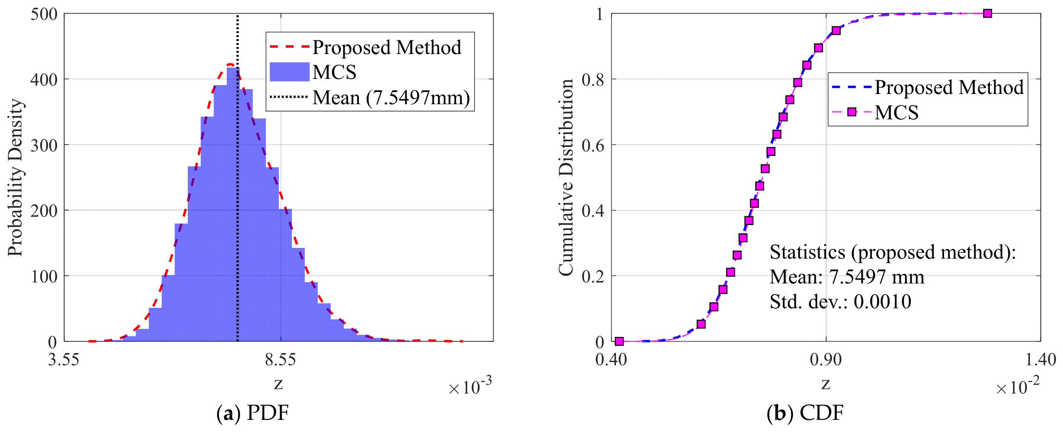
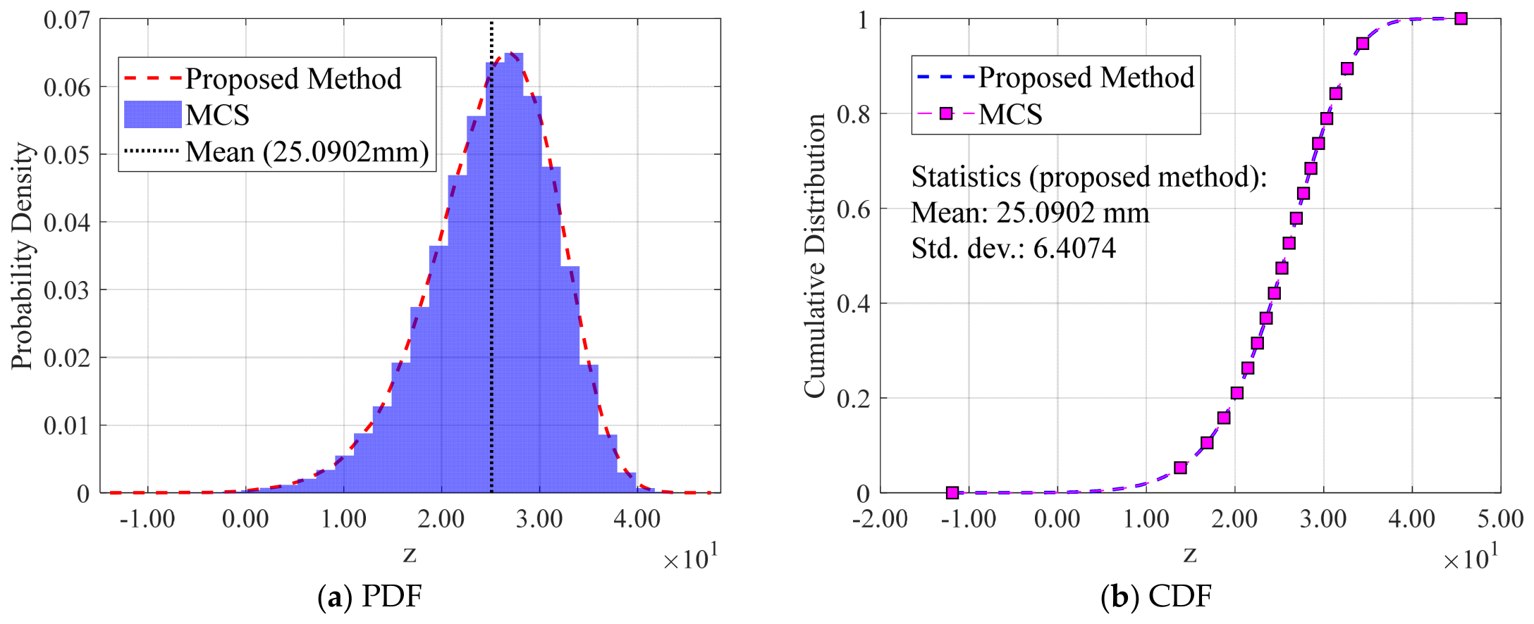
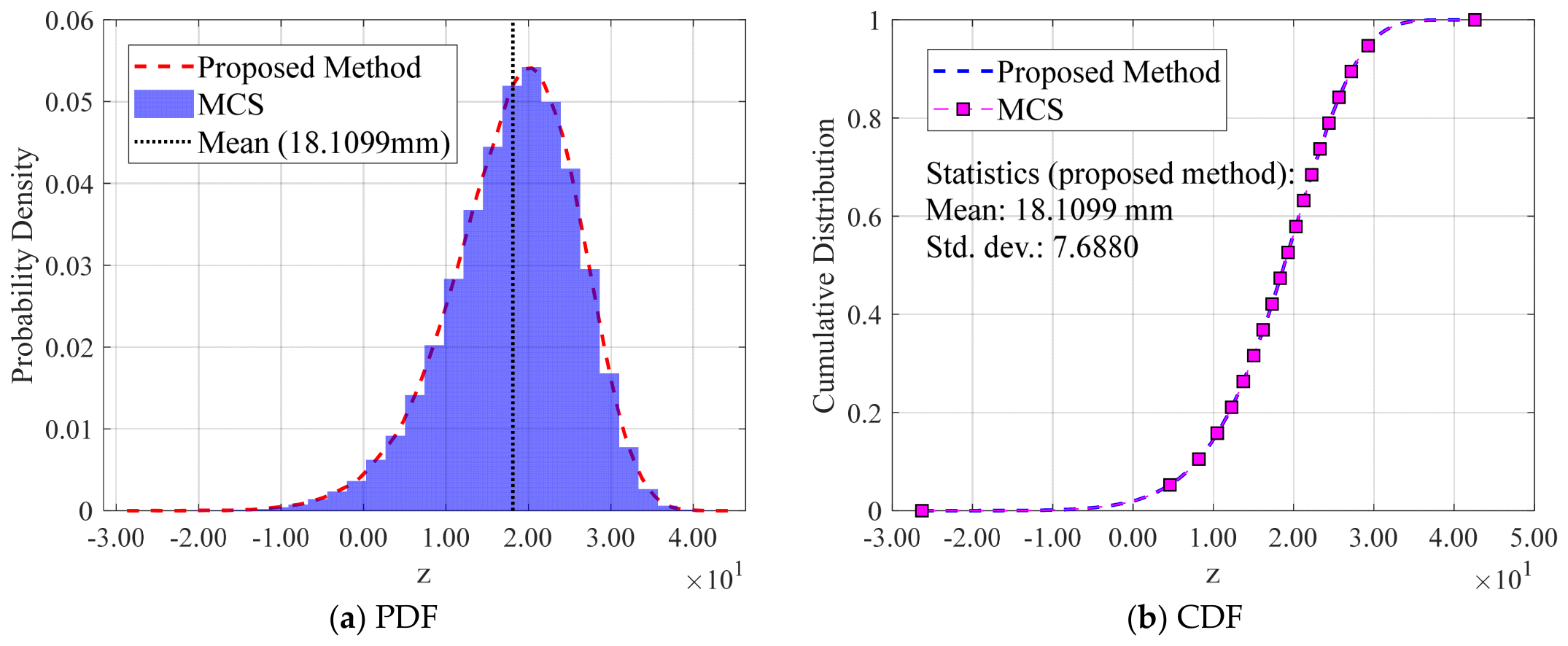
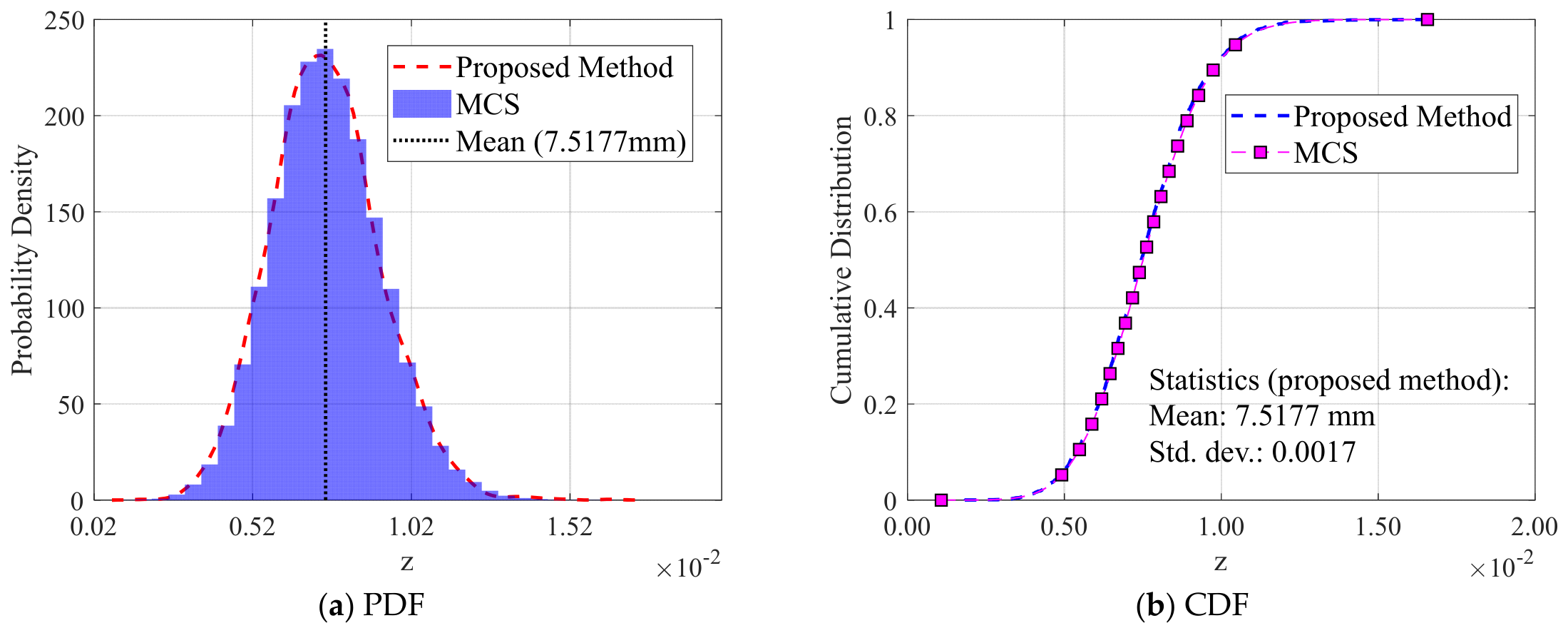
Following a comparison of the reliability indices and failure probabilities, the probabilistic characteristics of the structural response were further investigated. Figure 10 and Figure 11 show the probability density functions (PDFs) and cumulative distribution functions (CDFs) of the top-right node lateral displacement obtained from the proposed SVM-based framework and MCS under two representative load uncertainty levels. (Cv = 0.08 and Cv = 0.20).
As shown in Figure 10a,b and Figure 11a,b, the PDFs and CDFs predicted by the proposed method were in close agreement with the MCS results. The probability distributions obtained from both approaches nearly overlap, indicating that the proposed framework can accurately reproduce the statistical characteristics of the structural response even under different levels of load uncertainty.
To quantitatively assess the consistency between the two distributions, Kolmogorov–Smirnov (K-S) and Cramér-von Mises (C-M) goodness-of-fit tests were performed, and the results are summarized in Table 6. The K-S statistics are 0.0223 and 0.0227, with corresponding p-values of 0.1102 and 0.0982, respectively, both exceeding the significance level of 0.05. In addition, the C-M statistics are only 2.49 × 10⁻⁷ and 6.39 × 10⁻⁷, indicating excellent agreement between the predicted and reference distributions.
Following the accuracy validation of the proposed framework, its computational efficiency was further evaluated. The computational costs of the direct FE-based Monte Carlo simulation (FE-MCS) and the proposed SVM-assisted reliability methods were compared, including SVM-MCS, FORM-SVM, SORM (Breitung)-SVM, and SORM (Tvedt)-SVM. The results are summarized in Table 7.
As shown in Table 7, the direct FE-MCS approach requires 105 finite element evaluations, resulting in a total computational time of 674,995 s. In contrast, all SVM-based approaches require only 2000 FE evaluations to construct the surrogate model, after which reliability analyses are performed using a computationally efficient SVM surrogate. The total computational times of SVM-MCS, FORM-SVM, SORM (Breitung)-SVM, and SORM (Tvedt)-SVM are 13,505.47 s, 13,501.45 s, 13,501.47 s, and 13,501.48 s, respectively.
Compared with the direct FE-MCS, the proposed SVM-based framework reduces the computational cost by approximately 98% while maintaining a comparable reliability estimation accuracy. The results also indicate that the main computational burden of the proposed approach originates from the generation of FE training samples, whereas subsequent reliability calculations based on the SVM surrogate require negligible additional computational effort. Therefore, the proposed framework provides an efficient alternative for reliability analysis of nonlinear structures with computationally expensive implicit limit-state functions.

5.3. Example 3: A Three-Story Three-Span Rigid Frame Structure

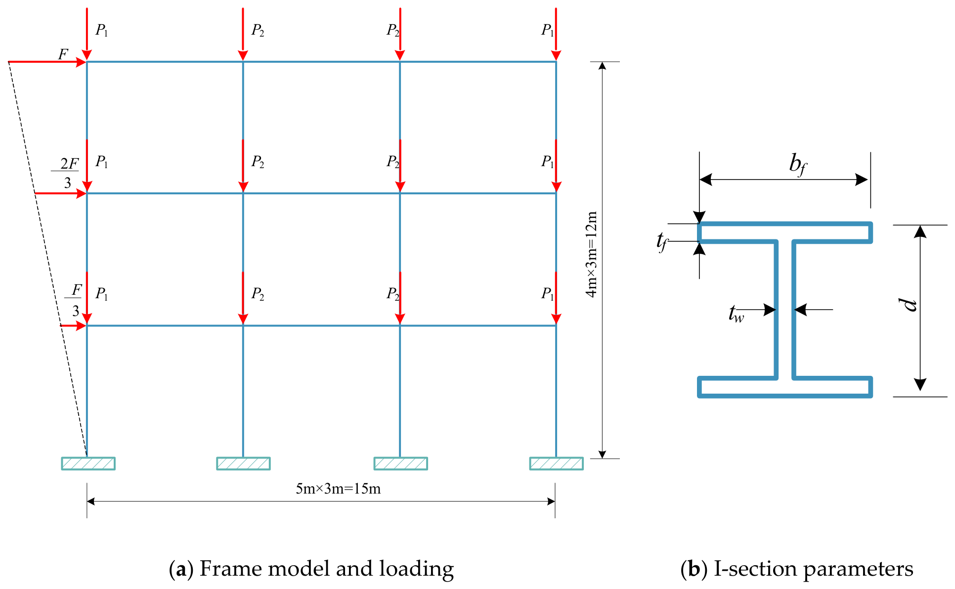
In this section, a planar frame structure is analyzed as a representative example. The frame consisted of three bays in the horizontal direction, each with a span of 5 m (total span 15 m), and three stories in the vertical direction, each 4 m high (total height 12 m). Concentrated horizontal and vertical loads were applied at each floor node, as illustrated in Figure 12a. Both the beams and columns adopt I-shaped cross-sections, with the section geometry shown in Figure 10b. The material behavior was modeled using an ideal elastic–perfectly plastic constitutive model. Under different loading conditions, the horizontal load was assumed to be a fixed proportion of the intermediate vertical load and was expressed as F = α P 2 ( α = 0.50 ,   0.55 ,   0.60 ,   0.65 ). The elastic modulus E of the structure, material yield strength f y , and horizontal and vertical loads applied at each floor are all treated as random variables, and their statistical parameters are listed in Table 8. A displacement limit of 60 mm is imposed on the top-level horizontal response. Using the proposed SVM-based limit-state function reconstruction method, the reliability of top-level horizontal displacement was evaluated using FORM and SORM. The resulting reliability indices and failure probabilities were compared with the MCS benchmarks.
Table 9 and Table 10 summarize the reliability indices and failure probabilities obtained using different reliability methods. As the load ratio increases from 0.50 to 0.65, the reliability index decreased continuously, whereas the corresponding failure probability increased, indicating the progressive deterioration of structural safety under increasing horizontal loading. This trend was consistently captured by all reliability methods. Compared with the MCS results, FORM generally yields slightly conservative reliability estimates owing to its first-order approximation of the limit-state surface. By incorporating second-order curvature information, both SORM formulations provided noticeably improved agreement with reference solutions. Among them, SORM (Tvedt) consistently produces the smallest deviations for both the reliability index and failure probability over the entire range of load ratios.
To evaluate the prediction accuracy quantitatively, the mean absolute errors and mean relative errors with respect to the MCS are summarized in Table 11. SORM methods substantially reduce prediction errors compared with FORM. In particular, SORM (Tvedt) achieves the lowest mean relative errors of only 0.08% for the reliability index and 0.58% for the failure probability, demonstrating its superior capability in representing the nonlinear characteristics of the limit-state surface.
To further verify the probabilistic characteristics of the reconstructed limit-state function, Figure 13 and Figure 14 compare the probability density functions (PDFs) and cumulative distribution functions (CDFs) of the top-story lateral displacement obtained from the proposed framework and MCS for two representative load ratios (α = 0.50 and α = 0.60). For both loading cases, the predicted PDFs closely match the MCS results in terms of both the distribution shape and peak location, while the corresponding CDF curves almost completely overlap over the entire probability range. These observations indicate that the proposed framework accurately reproduced the probabilistic characteristics of the structural response.
A quantitative comparison based on the Kolmogorov–Smirnov (K-S) and Cramér-von Mises (C-M) goodness-of-fit tests is presented in Table 12. For both load ratios, the K-S statistics remained below 0.023, with p-values greater than 0.05, indicating no statistically significant difference between the predicted and reference distributions. Meanwhile, the extremely small C–M statistics further confirmed the excellent agreement between the two probability distributions.
These results demonstrate that the proposed SVM-based framework not only provides accurate estimates of reliability indices and failure probabilities but also preserves the probabilistic characteristics of structural responses.
After validating the reliability prediction performance of the proposed framework, a comprehensive parametric study was further conducted to investigate the effects of different uncertainty sources on the reliability of nonlinear steel frames. Three representative types of uncertainties, including material properties, load parameters, and geometric parameters, were considered separately. For each case, only the investigated random variables were varied, while all other random variables were kept unchanged according to Table 8.
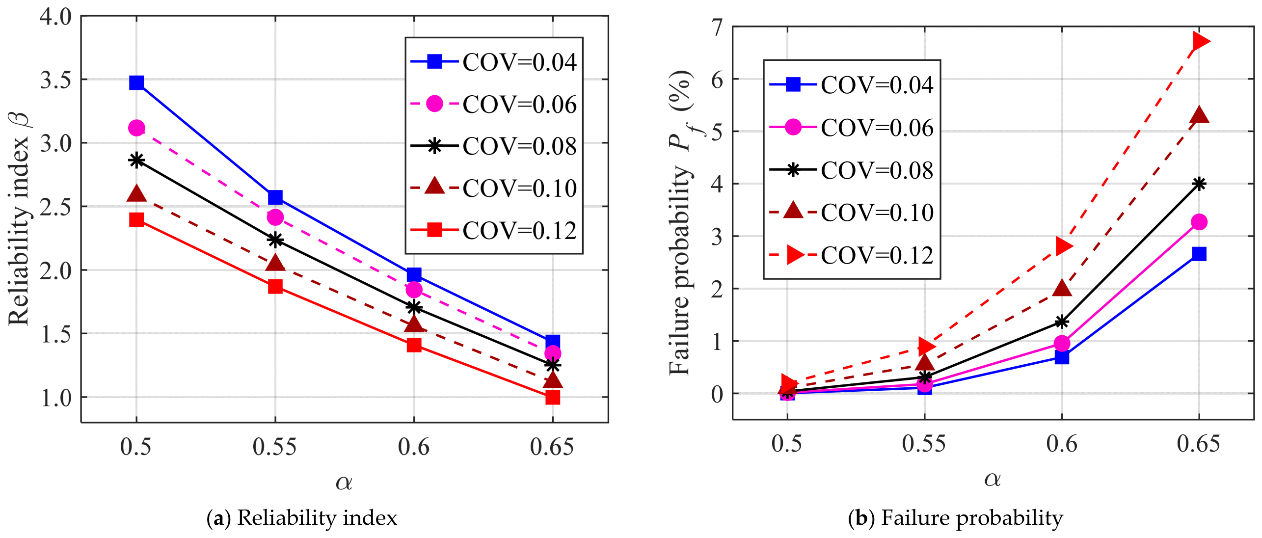
First, the effect of material uncertainty was investigated by simultaneously varying the coefficients of variation (COVs) of the elastic modulus and yield strength from 0.04 to 0.12 under different load ratios. The corresponding variations in reliability index and failure probability are presented in Figure 15. As shown in Figure 15a, the reliability index decreases continuously with increasing material uncertainty and load ratio, indicating that larger variability in material properties leads to a lower reliability level. Meanwhile, Figure 14b shows that the failure probability increases with increasing material uncertainty, and this trend becomes more evident under higher load ratios.
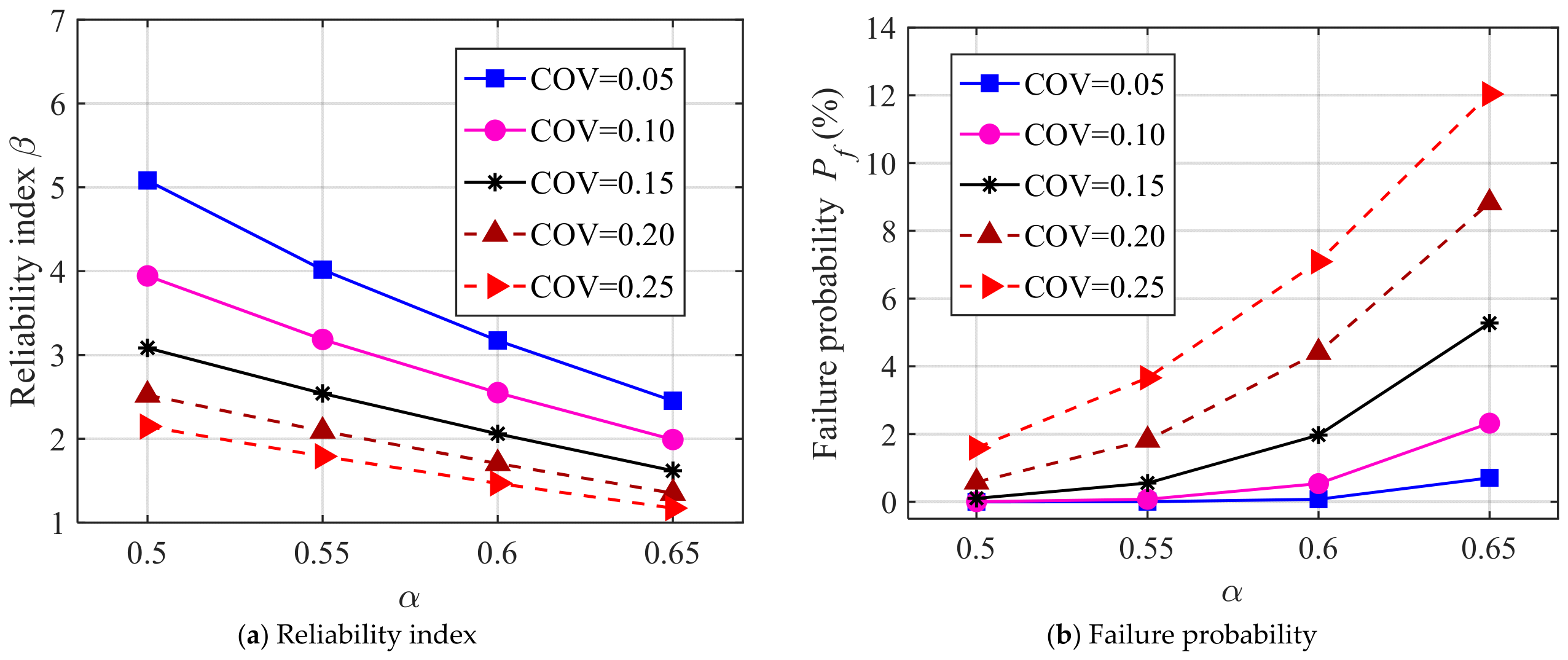
Second, the influence of load uncertainty was evaluated by simultaneously varying the COVs of horizontal and vertical loads from 0.05 to 0.25 under different load ratios, while material and geometric parameters remained unchanged. The results are presented in Figure 16. It can be observed that increasing load uncertainty leads to a gradual decrease in the reliability index and an increase in failure probability for all load ratios. Compared with material uncertainty, load variability produces a more pronounced effect on reliability degradation under high load levels, highlighting the importance of accurately considering load uncertainty in structural reliability assessment.
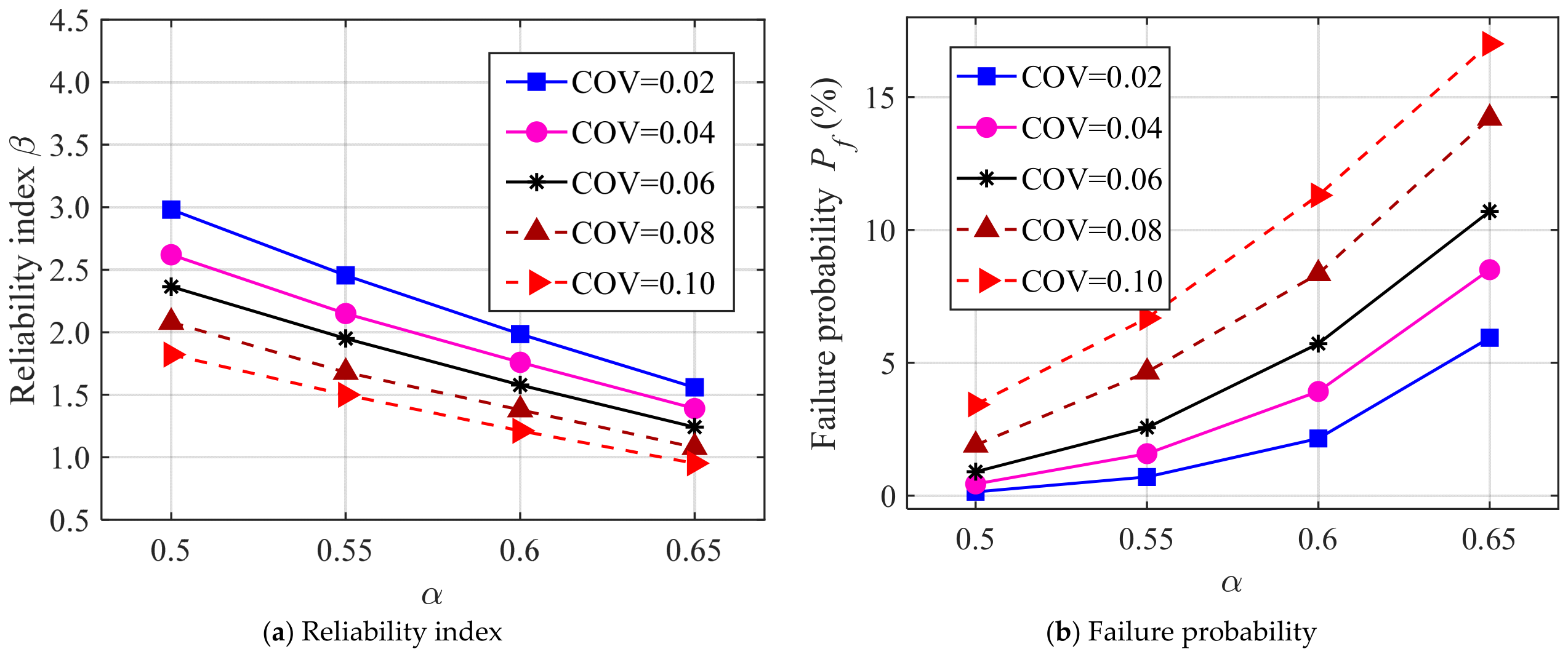
Furthermore, geometric uncertainty was considered by varying the story height and bay span parameters. The geometric parameters were assumed to follow normal distributions, with mean values of 4 m and 5 m for story height and bay span, respectively. The corresponding COV values ranged from 0.02 to 0.10, while the remaining random variables were unchanged. As shown in Figure 17, increasing geometric uncertainty results in a reduction in the reliability index and an increase in failure probability, demonstrating that geometric variability also contributes to the deterioration of structural reliability.
Overall, the comparative parametric analysis indicates that material, load, and geometric uncertainties have different influences on the reliability of nonlinear steel frames. Among the considered uncertainty sources, load uncertainty generally exhibits a relatively more pronounced effect on structural reliability, followed by material and geometric uncertainties.

6. Conclusions

This study addressed the challenge of efficiently evaluating nonlinear and implicit limit-state functions in structural reliability analysis by developing an SVM-based reconstruction framework integrated with conventional reliability methods. The SVM hyperparameters are optimized using particle swarm optimization (PSO), enabling the accurate approximation of nonlinear limit-state functions based on finite-element response samples. The reconstructed surrogate model was subsequently combined with FORM and SORM to evaluate the reliability of steel frame systems. The main conclusions are summarized as follows.
(1)
The proposed SVM-based reconstruction method effectively approximated nonlinear and implicit limit-state functions for the investigated benchmark functions and finite-element-based structural models. The reconstructed surrogate models exhibited high prediction accuracy, numerical stability, and good generalization capability, providing an explicit representation of the limit-state function for subsequent reliability analysis.
(2)
Integrating the reconstructed limit-state function with higher-order reliability methods improves the reliability estimation accuracy. Compared with FORM, SORM considers the curvature characteristics of the limit-state surface better and provides more accurate reliability indices and failure probabilities. Among the investigated approaches, SORM (Tvedt) achieved the closest agreement with the Monte Carlo simulation results.
(3)
For the nonlinear steel frame systems investigated in this study, the proposed framework effectively reduces computational costs while maintaining reliable prediction accuracy. The sensitivity analysis demonstrates that the proposed SVM-based reliability framework can achieve stable reliability predictions for planar steel frame structures with approximately 1500–2000 training samples.
(4)
Although the proposed framework shows satisfactory performance, further investigations are needed for more complex problems involving stronger nonlinearities, high-dimensional variables, and complex dependence structures.

Author Contributions

C.Y.: Methodology, Software, Validation, Formal analysis, Writing—Original Draft. J.W.: Conceptualization, Investigation, Supervision. D.B.: Conceptualization, Supervision, Resources, Writing-Reviewing and Editing. B.Z.: Conceptualization, Supervision. Y.F.: Conceptualization, Supervision, Funding Acquisition. All authors have read and agreed to the published version of the manuscript.

Funding

This research was funded by the Chongzuo City Science and Technology Plan (Grant Nos. 2024ZC018473 and 2026ZC0440), and the Guilin University of Technology 2024 Professional Classification Construction Project (Course: “Fundamentals of Steel Structures”). The APC was funded by the above-mentioned projects.

Institutional Review Board Statement

Not applicable.

Informed Consent Statement

Not applicable.

Data Availability Statement

The data that support the findings of this study are available upon reasonable request from the authors.

Acknowledgments

The financial support provided by the Chongzuo City Science and Technology Plan and the Guilin University of Technology 2024 Professional Classification Construction Project is gratefully acknowledged.

Conflicts of Interest

Author Bangzhi Zhang was employed by the company China Construction Eighth Engineering Division Corp., Ltd. The remaining authors declare that the research was conducted in the absence of any commercial or financial relationships that could be construed as a potential conflict of interest.

References

  1. Huang, X.; Li, Y.; Zhang, Y.; Zhang, X. A new direct second-order reliability analysis method. Appl. Math. Model. 2018, 55, 68–80. [Google Scholar] [CrossRef]
  2. Xu, J.; Dang, C. A new bivariate dimension reduction method for efficient structural reliability analysis. Mech. Syst. Signal Process. 2019, 115, 281–300. [Google Scholar] [CrossRef]
  3. Chen, W.; Gong, C.; Wang, Z.; Frangopol, D.M. Application of first-order reliability method with orthogonal plane sampling for high-dimensional series system reliability analysis. Eng. Struct. 2023, 282, 115778. [Google Scholar] [CrossRef]
  4. Dudzik, A.; Potrzeszcz-Sut, B. Hybrid approach to the first order reliability method in the reliability analysis of a spatial structure. Appl. Sci. 2021, 11, 648. [Google Scholar] [CrossRef]
  5. Kumar, P.; Samui, P.; Armaghani, D.J.; Roy, S.S. Second-order reliability analysis of an energy pile with CPT data. J. Build. Eng. 2024, 95, 110165. [Google Scholar] [CrossRef]
  6. Hu, Z.; Mansour, R.; Olsson, M.; Du, X. Second-order reliability methods: A review and comparative study. Struct. Multidiscip. Optim. 2021, 64, 3233–3263. [Google Scholar] [CrossRef]
  7. Chen, Z.; Qiu, G.; Li, X.; Yang, Z.; Chen, G.; Gan, X. An improved approximate integral method for nonlinear reliability analysis. Comput. Methods Appl. Mech. Eng. 2024, 429, 117158. [Google Scholar] [CrossRef]
  8. Grubišić, M.; Ivošević, J.; Grubišić, A. Reliability analysis of reinforced concrete frame by finite element method with implicit limit state functions. Buildings 2019, 9, 119. [Google Scholar] [CrossRef]
  9. Liu, B.; Xie, L. An improved structural reliability analysis method based on local approximation and parallelization. Mathematics 2020, 8, 209. [Google Scholar] [CrossRef]
  10. Zhao, J.; Cui, D.; Zhao, Q. Structural reliability analysis of improved response surface method based on maximum entropy principle. Proc. Inst. Mech. Eng. Part O J. Risk Reliab. 2026, 240, 582–598. [Google Scholar] [CrossRef]
  11. Gao, S.; Zhao, Y.; Zhao, X.; Zhang, Y. Application of response surface method based on new strategy in structural reliability analysis. Structures 2023, 57, 105202. [Google Scholar] [CrossRef]
  12. Lim, H.U.; Manuel, L. Distribution-free polynomial chaos expansion surrogate models for efficient structural reliability analysis. Reliab. Eng. Syst. Saf. 2021, 205, 107256. [Google Scholar] [CrossRef]
  13. Le, V.; Caracoglia, L. A neural network surrogate model for the performance assessment of a vertical structure subjected to non-stationary, tornadic wind loads. Comput. Struct. 2020, 231, 106208. [Google Scholar] [CrossRef]
  14. Schweizer, M.; Fina, M.; Wagner, W.; Freitag, S. Artificial neural networks for random fields to predict the buckling load of geometrically imperfect structures. Comput. Mech. 2025, 76, 181–204. [Google Scholar] [CrossRef]
  15. Yang, S.; He, Z.; Chai, J.; Meng, D.; Macek, W.; Branco, R.; Zhu, S.-P. A novel hybrid adaptive framework for support vector machine-based reliability analysis: A comparative study. Structures 2023, 58, 105665. [Google Scholar] [CrossRef]
  16. Roy, A.; Chakraborty, S. Support vector machine in structural reliability analysis: A review. Reliab. Eng. Syst. Saf. 2023, 233, 109126. [Google Scholar] [CrossRef]
  17. Funk, S.; Airoud Basmaji, A.; Nackenhorst, U. Globally supported surrogate model based on support vector regression for nonlinear structural engineering applications. Arch. Appl. Mech. 2023, 93, 825–839. [Google Scholar] [CrossRef]
  18. Zhao, H.; Li, S.; Ru, Z. Adaptive reliability analysis based on a support vector machine and its application to rock engineering. Appl. Math. Model. 2017, 44, 508–522. [Google Scholar] [CrossRef]
  19. Karahan, H.; Alkaya, D. Integrating SVR Optimization and Machine Learning-Based Feature Importance for TBM Penetration Rate Prediction. Appl. Sci. 2025, 16, 355. [Google Scholar] [CrossRef]
  20. Bliek, L.; Guijt, A.; Karlsson, R.; Verwer, S.; de Weerdt, M. Benchmarking surrogate-based optimisation algorithms on expensive black-box functions. Appl. Soft Comput. 2023, 147, 110744. [Google Scholar] [CrossRef]
  21. Kaloop, M.R.; Kumar, D.; Samui, P.; Gabr, A.R.; Hu, J.W.; Jin, X.; Roy, B. Particle swarm optimization algorithm-extreme learning machine (PSO-ELM) model for predicting resilient modulus of stabilized aggregate bases. Appl. Sci. 2019, 9, 3221. [Google Scholar] [CrossRef]
  22. Li, F.; Li, Y.; Cai, X.; Gao, L. A surrogate-assisted hybrid swarm optimization algorithm for high-dimensional computationally expensive problems. Swarm Evol. Comput. 2022, 72, 101096. [Google Scholar] [CrossRef]
  23. Dong, Y.; Chen, Z.; Zhao, Y. Hybrid genetic algorithm with interpretable surrogate modeling for enhanced optimization of short-fiber reinforced polymer composites. Mater. Des. 2025, 258, 114611. [Google Scholar] [CrossRef]
  24. Bai, R.; Liang, G.; Cheng, H.; Naceur, H.; Coutellier, D.; Zhao, J.; Luo, J.; Pu, H.; Yi, J. Optimizing additive manufacturing path pattern for Ti-6Al-4V thin rods using a combinatorial radial basis function surrogate-assisted genetic algorithm. Mater. Des. 2023, 236, 112447. [Google Scholar] [CrossRef]
  25. Pepper, N.; Crespo, L.; Montomoli, F. Adaptive learning for reliability analysis using support vector machines. Reliab. Eng. Syst. Saf. 2022, 226, 108635. [Google Scholar] [CrossRef]
  26. Tvedt, L. Second order reliability by an exact integral. In Reliability and Optimization of Structural Systems ’88: Proceedings of the 2nd IFIP WG7.5 Conference London, UK, September 26–28, 1988; Springer: Berlin/Heidelberg, Germany, 1988; pp. 377–384. [Google Scholar] [CrossRef]
  27. Lee, I.; Noh, Y.; Yoo, D. A novel second-order reliability method (SORM) using noncentral or generalized chi-squared distributions. J. Mech. Des. 2012, 134, 100912. [Google Scholar] [CrossRef]
  28. Mansour, R.; Olsson, M. A closed-form second-order reliability method using noncentral chi-squared distributions. J. Mech. Des. 2014, 136, 101402. [Google Scholar] [CrossRef]
  29. Li, H.S.; Lü, Z.Z.; Yuan, X.K. Nataf transformation based point estimate method. Chin. Sci. Bull. 2008, 53, 2586–2592. [Google Scholar] [CrossRef]
  30. Xiao, Q. Evaluating correlation coefficient for Nataf transformation. Probabilistic Eng. Mech. 2014, 37, 1–6. [Google Scholar] [CrossRef]
  31. Hasofer, A.M.; Lind, N.C. An exact and invarient first order reliability format. J. Eng. Mech. Div. 1974, 100, 111–121. [Google Scholar]
  32. Keshtegar, B.; Meng, Z. A hybrid relaxed first-order reliability method for efficient structural reliability analysis. Struct. Saf. 2017, 66, 84–93. [Google Scholar] [CrossRef]
  33. Breitung, K. Asymptotic approximations for multinormal integrals. J. Eng. Mech. 1984, 110, 357–366. [Google Scholar] [CrossRef]
  34. Zhou, T.; Peng, Y. Kernel principal component analysis-based Gaussian process regression modelling for high-dimensional reliability analysis. Comput. Struct. 2020, 241, 106358. [Google Scholar] [CrossRef]
  35. Su, G.; Peng, L.; Hu, L. A Gaussian process-based dynamic surrogate model for complex engineering structural reliability analysis. Struct. Saf. 2017, 68, 97–109. [Google Scholar] [CrossRef]
  36. Zhao, H. Slope reliability analysis using a support vector machine. Comput. Geotech. 2008, 35, 459–467. [Google Scholar] [CrossRef]
  37. Li, H.; Lü, Z.; Yue, Z. Support vector machine for structural reliability analysis. Appl. Math. Mech. 2006, 27, 1295–1303. [Google Scholar] [CrossRef]
  38. Wu, J.; Wang, Y.G. A working likelihood approach to support vector regression with a data-driven insensitivity parameter. Int. J. Mach. Learn. Cybern. 2023, 14, 929–945. [Google Scholar] [CrossRef]
  39. Smola, A.J.; Schölkopf, B. A tutorial on support vector regression. Stat. Comput. 2004, 14, 199–222. [Google Scholar] [CrossRef]
  40. Thurnhofer-Hemsi, K.; López-Rubio, E.; Molina-Cabello, M.A.; Najarian, K. Radial basis function kernel optimization for support vector machine classifiers. arXiv 2020, arXiv:2007.08233. [Google Scholar] [CrossRef]
  41. Elgeldawi, E.; Sayed, A.; Galal, A.R.; Zaki, A.M. Hyperparameter tuning for machine learning algorithms used for arabic sentiment analysis. Informatics 2021, 8, 79. [Google Scholar] [CrossRef]
  42. Gavin, H.P.; Yau, S.C. High-order limit state functions in the response surface method for structural reliability analysis. Struct. Saf. 2008, 30, 162–179. [Google Scholar] [CrossRef]
  43. Radoń, U.; Zabojszcza, P. The application of structural reliability and sensitivity analysis in engineering practice. Appl. Sci. 2025, 15, 342. [Google Scholar] [CrossRef]
  44. Tvedt, L. Distribution of quadratic forms in normal space-application to structural reliability. J. Eng. Mech. 1990, 116, 1183–1197. [Google Scholar] [CrossRef]
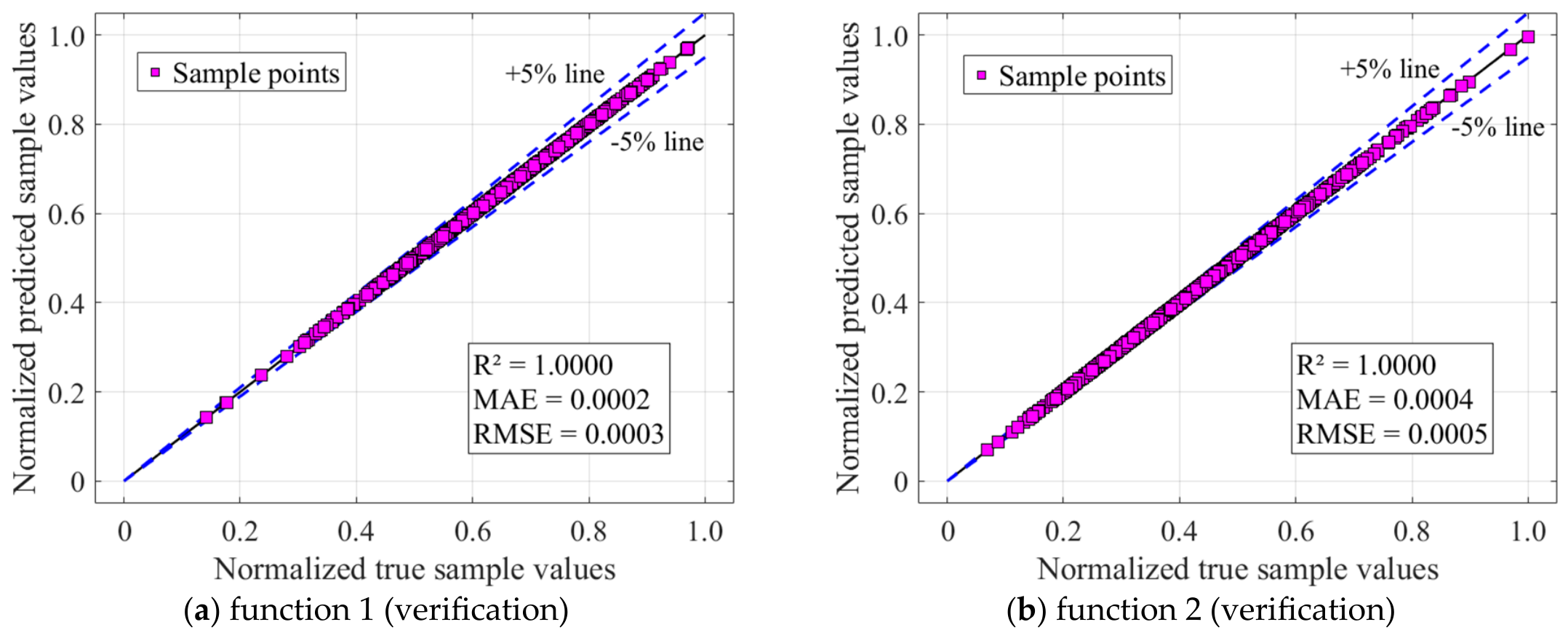
Figure 1. Prediction performance of the SVM-based reconstructed limit state function.
Applsci 16 07699 g001
Figure 2. 10-fold cross-validation results of the SVM-reconstructed limit-state function.
Applsci 16 07699 g002
Figure 3. Sensitivity analysis of reliability prediction errors with respect to training sample size for the SVM-reconstructed limit-state functions.
Applsci 16 07699 g003
Figure 4. Loads and dimensions of the five-storey three-bay rigid frame.
Applsci 16 07699 g004
Figure 5. Sensitivity analysis of the SVM-reconstructed limit-state function with respect to training sample size under different load uncertainty levels.
Applsci 16 07699 g005
Figure 6. Prediction performance of the SVM-reconstructed limit-state function under different load uncertainty levels.
Applsci 16 07699 g006
Figure 7. Convergence of reliability indices with increasing training sample size under different load uncertainty levels.
Applsci 16 07699 g007
Figure 8. Relative errors of reliability indices (β) obtained from SORM methods with respect to MCS results.
Applsci 16 07699 g008
Figure 9. Relative errors of failure probability (Pf) obtained from SORM methods with respect to MCS results.
Applsci 16 07699 g009
Figure 10. Probability distribution comparison of the top-right node displacement under Cv = 0.08: (a) PDF and (b) CDF.
Applsci 16 07699 g010
Figure 11. Probability distribution comparison of the top-right node displacement under Cv = 0.20: (a) PDF and (b) CDF.
Applsci 16 07699 g011
Figure 12. A three-story three-bay steel frame structure.
Applsci 16 07699 g012
Figure 13. Probability distribution comparison of the top-right node lateral displacement of the rigid-frame structure under α = 0.50: (a) PDF and (b) CDF.
Applsci 16 07699 g013
Figure 14. Probability distribution comparison of the top-right node lateral displacement of the rigid-frame structure under α = 0.60: (a) PDF and (b) CDF.
Applsci 16 07699 g014
Figure 15. Effects of material uncertainty on structural reliability under different load factors.
Applsci 16 07699 g015
Figure 16. Effects of load uncertainty on structural reliability under different load factors.
Applsci 16 07699 g016
Figure 17. Effects of geometry uncertainty on structural reliability under different load factors.
Applsci 16 07699 g017
Table 1. The reliability indices and failure probabilities obtained by different methods.
FunctionComputational
Content
FORMSORM
(Breitung)
SORM
(Tvedt)
MCSResult Source
Function 1Reliability indices2.3492.2582.2482.251Proposed Method
Failure probability P f 9.422 × 10−31.197 × 10−21.229 × 10−21.218 × 10−2
Reliability indices2.3482.2502.241-Tvedt [44]
Failure probability P f 9.433 × 10−31.222 × 10−21.253 × 10⁻²-
Penalty coefficient C 25.2834
Insensitive loss coefficient ε 0.0010
Kernel function parameter γ 6.3989
Function 2Reliability indices2.0382.1592.1842.188Proposed Method
Failure probability P f 2.0797 × 10⁻² 1.5408 × 10⁻² 1.4472 × 10⁻² 1.4352 × 10⁻²
Reliability indices2.055-2.1882.190Lee et al.
[27]
Failure probability P f 2.0477 × 10⁻²-1.4409 × 10−21.4301 × 10−2
Penalty coefficient C 28.9452
Insensitive loss coefficient ε 0.0010
Kernel function parameter γ 3.7106
Table 2. The statistical properties of the random variables in Example 2.
VariableDistributionMeanCoefficient of
Variation
Dimension
E Lognormal2000.1GPa
f y Lognormal2480.1MPa
P 1 Normal300.05–0.20kN
P 2 Normal1000.05–0.20kN
q Normal180.05–0.20kN
Table 3. Comparison of reliability indices obtained from different reliability methods.
Coefficient of VariationFORMSORM
(Breitung)
SORM
(Tvedt)
MCS
0.052.5502.5672.5692.572
0.082.2452.2652.2682.273
0.111.9631.9841.9881.993
0.141.7251.7451.7501.753
0.171.5551.5461.5521.555
0.201.3641.3821.3881.389
Table 4. Comparison of failure probabilities obtained from different reliability methods.
Coefficient of VariationFORMSORM
(Breitung)
SORM
(Tvedt)
MCS
0.055.3923 × 10−35.1305 × 10−35.0978 × 10−35.0703 × 10⁻³
0.081.2398 × 10−21.1771 × 10−21.1674 × 10−21.1513 × 10⁻²
0.112.4804 × 10−22.3623 × 10−22.3396 × 10−22.3131 × 10⁻²
0.144.2284 × 10−24.0473 × 10−24.0047 × 10−23.9777 × 10⁻²
0.176.3371 × 10−26.0995 × 10−26.0320 × 10−25.9989 × 10⁻²
0.208.6277 × 10−28.3514 × 10−28.2583 × 10−28.2487 × 10⁻²
Table 5. Quantitative error comparison of reliability methods with respect to MCS results.
MethodMean Absolute Error (β)Mean Relative Error of β (%)Mean Absolute Error (Pf × 10−3)Mean Relative Error of Pf (%)
FORM0.02181.112.15 × 10−34.56
SORM (Breitung)0.01050.540.82 × 10−31.74
SORM (Tvedt)0.00400.200.24 × 10−30.52
Table 6. Quantitative comparison of distribution consistency between the proposed method and MCS.
ComparisonK-S Statisticp-ValueC-M Statistic
Proposed vs. Monte Carlo (Cv = 0.08)0.02230.11022.49 × 10−7
Proposed vs. Monte Carlo (Cv = 0.20)0.02270.09826.39 × 10−7
Table 7. Computational efficiency comparison between direct FE-MCS and SVM-assisted reliability analysis methods.
MethodNumber of FE
Calls
Number of SVM
Evaluations
Computational Time (s)
FE-MCS105674,995
SVM-MCS200010513,499.9 + 5.57 = 13,505.47
FORM-SVM200013,499.9 + 1.56 = 13,501.45
SORM (Breitung)-SVM200013,499.9 + 1.58 = 13,501.47
SORM (Tvedt)-SVM200013,499.9 + 1.59 = 13,501.48
Note: The computational time of the SVM-based methods includes the time required to generate 2000 FE training samples and subsequent reliability analysis. For example, 13,499.9 + 5.57 = 13,505.47 s represents the FE evaluation time (13,499.9 s) plus the SVM-MCS analysis time (5.57 s). Similar definitions were applied to FORM-SVM and SORM-SVM.
Table 8. The statistical properties of the random variables in Example 3.
VariableDistributionMeanCoefficient of VariationDimension
E Lognormal2000.10GPa
f y Lognormal2480.10MPa
P 1 Lognormal500.15kN
P 2 Lognormal1000.15kN
F Lognormal α P 2 (50, 55, 60, 65)0.15kN
Table 9. The reliability indices obtained by different analysis methods.
Load Ratio
α
FORMSORM
(Breitung)
SORM
(Tvedt)
MCS
0.503.0693.0843.0853.088
0.552.5342.5402.5412.544
0.602.0542.0572.0602.061
0.651.6231.6201.6191.618
Table 10. The failure probabilities obtained by different analysis methods.
Load Ratio
α
FORMSORM
(Breitung)
SORM
(Tvedt)
MCS
0.501.0750 × 10−31.0224 × 10−31.0176 × 10−31.0070 × 10⁻³
0.555.6317 × 10−35.5443 × 10−35.5333 × 10−35.4837 × 10⁻³
0.601.9988 × 10−21.9843 × 10−21.9699 × 10−21.9652 × 10⁻²
0.655.2275 × 10−25.2662 × 10−25.2762 × 10−25.2831 × 10⁻²
Table 11. The quantitative comparison of the prediction errors with respect to the MCS for different load ratios.
MethodMean Absolute Error (β)Mean Relative Error of β (%)Mean Absolute Error (Pf × 10−3)Mean Relative Error of Pf (%)
FORM0.01030.410.2773.05
SORM (Breitung)0.00350.150.1090.98
SORM (Tvedt)0.00200.080.0440.58
Table 12. The quantitative comparison of the prediction errors with respect to the MCS.
ComparisonK–S Statisticp-ValueC-M Statistic
Proposed vs. Monte Carlo (α = 0.50)0.02230.11022.49 × 10−7
Proposed vs. Monte Carlo (α = 0.60)0.02270.09826.39 × 10−7
Disclaimer/Publisher’s Note: The statements, opinions and data contained in all publications are solely those of the individual author(s) and contributor(s) and not of MDPI and/or the editor(s). MDPI and/or the editor(s) disclaim responsibility for any injury to people or property resulting from any ideas, methods, instructions or products referred to in the content.