Article

A Methodology for Adaptive Design of Fractal Neural Architectures for Forecasting Self-Similar and Multifractal Time Series


by
Nataliya Shakhovska
,
Volodymyr Shymanskyi
* and
Andrii Maherovskyi
Department of Artificial Intelligence, Lviv Polytechnic National University, 79905 Lviv, Ukraine
*
Author to whom correspondence should be addressed.
Appl. Sci. 2026, 16(15), 7563; https://doi.org/10.3390/app16157563
Submission received: 7 July 2026 / Revised: 24 July 2026 / Accepted: 27 July 2026 / Published: 30 July 2026

Abstract

Conventional recurrent and convolutional-recurrent neural architectures are often effective in capturing local and sequential dependencies. However, they may be insufficient for representing hierarchical scale-dependent structures that occur in time series with fractal or multifractal properties. This study addresses this limitation by modifying the FractalNet-LSTM architecture through the modification of its fractal block. Rather than treating the fractal block as a fixed component, the proposed approach introduces parametric branching, which allows the number of parallel computational paths to be adapted to the structural complexity of the analyzed time series. The study evaluates the proposed architecture on three time series datasets from different domains. Prior to model training, the datasets were analyzed using methods to assess self-similarity, long-range dependence, and multifractal properties. The forecasting performance of the modified FractalNet-LSTM was compared with LSTM, BiLSTM, CNN-LSTM, and the classical FractalNet-LSTM model across several forecasting horizons. The experimental results indicate that the proposed architecture can improve forecasting accuracy for time series with pronounced fractal and multifractal characteristics. The advantage is most evident for datasets with heterogeneous scale-dependent behavior, while the improvement is less pronounced for weakly multifractal or near-monofractal series. For example, on the Industrial Boiler dataset, the proposed model increased R2 from 0.8046 to 0.9195 for the 8-step horizon compared with the classical FractalNet-LSTM. On the Green Energy Demand dataset, R2 increased from 0.9316 to 0.9808 for the 1-step horizon and from 0.7357 to 0.8445 for the 8-step horizon. The results indicate that shorter forecasting horizons may require fewer branches, whereas longer horizons and more complex multifractal structures may benefit from deeper or more expressive fractal blocks.

1. Introduction

1.1. Related Work

Time-series forecasting is widely used in energy, finance, healthcare, road traffic analysis, industrial production, and meteorology. It supports the prediction of trends, volatility, seasonal variations, and other temporal patterns that are important for decision-making and resource allocation [1,2]. Classical statistical models, such as autoregressive integrated moving average (ARIMA) and seasonal ARIMA (SARIMA), remain widely used for time-series forecasting [3]. However, their effectiveness may be limited when the analyzed data are nonlinear, nonstationary, or characterized by complex temporal dependencies, which are common properties of real-world time series [4].
Recent studies have investigated hybrid neural architectures to improve forecasting accuracy for complex temporal data. For example, hybrid recurrent models combining conventional forecasting methods with gated recurrent units (GRUs) have demonstrated improved performance in capturing nonlinear temporal patterns [5]. Other studies have explored the use of fractal concepts in deep learning, including anomaly detection in fractal time series using LSTM-based autoencoders [6]. These works indicate the potential of combining neural architectures with structural properties of time series, but the design of neural models for explicitly self-similar and multifractal data remains insufficiently explored.
Nevertheless, despite the advances made in all the previously mentioned works, challenges remain in capturing complex temporal patterns. This is particularly evident in time series with pronounced self-similar and hierarchical structures. When the data exhibits strong non-stationary behavior or pronounced nonlinearity, this becomes evident in the forecasting models. If the patterns are complex and large-scale, they can pose challenges for both basic models such as ARIMA and SARIMA, as well as more complex models like RNNs [7]. Therefore, it is necessary to employ approaches that effectively handle the self-similar and hierarchical nature of time series, which requires an additional level of feature extraction at various levels of abstraction. Fractal neural networks, renowned for their effectiveness in such tasks, can serve as a solution to this problem.
To a certain extent, fractal neural networks can be considered a new approach to deep learning, as they are distinguished by the combination of fractal geometry [8] with neural networks [9], unlike other approaches. The presence of a hierarchical structure and self-similarity ensures that fractal neural networks are highly effective in modeling complex patterns and nonlinear dependencies. This feature is particularly useful for time series with long-term and cyclical dependencies [10]. According to recent studies, fractal neural networks have significant potential for improving noise robustness as well as enhancing the models’ generalization ability [11].
Fractal geometry is a branch of mathematics that studies self-similar patterns repeating at different scales and forming complex hierarchical structures. For this reason, parallel branches (e.g., Conv1D) or transformations are introduced in fractal neural networks, which can operate at different levels of abstraction, all thanks to the principle of self-similarity. The merging of branches is designed for multiscale feature representation and is typically implemented through averaging and concatenation. A structure consisting of many branches, where each parallel path performs similar operations and aligns with the concept of self-similarity inherent in fractal geometry, is called a fractal design. The effective capture of patterns across different time scales is the main strength of fractal neural networks [12]. These properties allow fractal architectures to represent multiscale temporal structure that conventional sequential architectures capture less effectively.
Beyond recurrent architectures, several specialised deep-learning models have recently been proposed for time-series forecasting. Temporal convolutional networks (TCNs) rely on dilated causal convolutions to obtain a large receptive field and capture long-range dependencies without recurrence [13,14]. Feed-forward residual models such as N-BEATS and its hierarchical successor N-HiTS achieve competitive accuracy on standard forecasting benchmarks using only backward and forward residual stacks [15,16]. More recently, Transformer-based forecasters, including Informer, Autoformer, and PatchTST, apply self-attention mechanisms to long-horizon prediction and currently represent the state of the art on several benchmarks [17,18,19]. These families differ fundamentally from the recurrent networks used as baselines in the present study. Recurrent models (LSTM, BiLSTM, and CNN-LSTM) were nonetheless adopted as the comparison set because the proposed method combines the modified fractal block with an LSTM head; an LSTM-based baseline therefore isolates the contribution of the fractal block itself. A broader empirical comparison against convolutional, residual, and attention-based forecasters is left for future work.

1.2. Motivation and Contributions

Despite progress in time-series forecasting, the relationship between measurable fractal or multifractal properties of a time series and the internal design of a neural forecasting architecture remains insufficiently explored. It is important to recognize that the use of fractal neural networks in time series forecasting has not yet been sufficiently studied. This is why there is a need to integrate neural network architectures with fractal properties. In theory, this will positively impact forecasting accuracy and help overcome the limitations of existing methods [20,21].
Experiments comparing fractal neural networks with other deep learning methods already exist [22]. The results reported in that study showed cases in which established approaches performed better, as well as cases in which the proposed method prevailed. These mixed outcomes indicate that the conditions under which fractal architectures are advantageous are not yet well established, which motivates further systematic investigation.
The major contributions of our study are as follows:
(1)
This study adapts the fractal neural design to one-dimensional time-series forecasting and treats the number of branches in the fractal block as an explicit tunable architectural parameter. Since classical FractalNet already uses parallel paths, the novelty of this work is not the mere presence of multiple branches, but the use of branch count as a data-dependent design variable related to the self-similarity and multifractality of the target series. In the proposed modified fractal block, several parallel Conv1D paths are aggregated and passed to an LSTM head that models temporal dependencies.
(2)
The study systematically examined how different branching configurations of the modified fractal block affect forecasting accuracy across short-, medium-, and longer-term prediction horizons.
(3)
The proposed FractalNet-LSTM architecture with a modified fractal block was compared with LSTM, BiLSTM, CNN-LSTM, and the classical FractalNet-LSTM model using several forecasting accuracy metrics. The experiments were conducted on three time series datasets from different domains.
(4)
The study provides empirical evidence that fractal neural architectures are suitable for forecasting time series with pronounced self-similar and multifractal properties. The results support the hypothesis that the internal structure of a forecasting model should be selected with regard to the structural properties of the analyzed time series.
The remainder of the paper is organized as follows: Section 2 presents the materials and methods used in this study. It includes a description of the approaches for assessing self-similarity, long-range dependence, and multifractality of time series. This section also describes the forecasting models used for comparison and the proposed FractalNet-LSTM model with a modified fractal block based on parametric branching. Section 3 reports the experimental results. Section 4 discusses the obtained results and interprets them in the context of the structural properties of the analyzed time series. Finally, Section 5 summarizes the main findings of the study and outlines priority directions for future research.

2. Materials and Methods

2.1. Methods for Assessing Self-Similarity and Multifractality of Time Series

The study of self-similarity and multifractality of time series is a very important stage, as it allows one to reveal the deep scale structure of the process, the presence of long-term memory, persistence, nonlinearity and heterogeneity of fluctuations on different time scales. Taking into account these properties allows one to reasonably choose the appropriate class of forecasting models, to avoid simplified assumptions about the independence or stationarity of data, to increase the accuracy and stability of forecasts, and to reduce the risk of obtaining biased or unstable estimates of model parameters.
The DFA (Detrended Fluctuation Analysis) method is used to estimate the scaling exponent α, which characterizes the long-term correlations and self-similarity of a time series. The method was proposed by Peng et al. [23,24] to analyze fractal scaling in time series.
α = d log F ( s ) d log s ,
The Abry–Veitch method uses a discrete wavelet transform to estimate the Hurst parameter H based on the large-scale behavior of the dispersion of the wavelet coefficients [25]. This approach is widely used for the analysis of long-range dependence.
H = β − 1 2 ,
The GPH (Geweke–Porter–Hudak) method is used for semiparametric estimation of the fractional integration parameter d in long-memory processes [26]. It is based on log-periodogram regression in the low-frequency domain. In Equation (3), I(λj) is the periodogram of the series evaluated at the Fourier frequencies λj = 2πj/n (j = 1, …, m, with m ≪ n), c is a constant, εj is the regression error, and the memory parameter d is estimated as the negative ordinary-least-squares slope of ln I(λj) regressed on ln(4 sin2(λj/2)).
l n   I ( λ j ) = c − d   l n ( 4   s i n 2 ( λ j 2 ) ) + ε j ,
MF-DFA (Multifractal Detrended Fluctuation Analysis) is a generalization of DFA for studying multifractality. The method allows us to estimate the dependence of the generalized Hurst exponent h(q) on the moment order q. If h(q) varies with q, the series has a multifractal structure.
α ( q ) = d τ ( q ) d q ,
∆ α = α m a x − α m i n ,
∆ h = h q m i n − h ( q m a x ) ,
The Wavelet Leaders method, developed by Jaffard et al. [25,27], is a theoretically rigorous approach to multifractal analysis based on the supremums of wavelet coefficients in the influence cone. The scaling structure function ζ(q) and the singularity spectrum f(α) are obtained through the standard Legendre transformation.
α ( q ) = d ζ ( q ) d q ,
∆ ζ = ζ q m i n − ζ ( q m a x ) ,
The integrated use of DFA, Abry–Veitch, GPH, MF-DFA and Wavelet Leaders methods is relevant and appropriate, as they allow us to study various aspects of the large-scale structure of time series. DFA, Abry–Veitch and GPH are mainly focused on assessing self-similarity and long-term memory, while MF-DFA and Wavelet Leaders provide an in-depth analysis of multifractal properties. The combination of these approaches increases the reliability of the estimation of the Hurst parameter, allows us to detect hidden patterns in complex systems and provides a more complete understanding of the nature of the processes under study.

2.2. Time Series Forecasting Models

Several methods were employed in this study to ensure a more objective comparison of results. Therefore, each of these methods was used in the training and subsequent analysis of the results. The approaches used in this study include BILSTM, CNN-LSTM, LSTM, FractalNet-LSTM, and the proposed FractalNet-LSTM solution with a modified fractal block.
The first method used for comparison in this paper is LSTM. Long Short-Term Memory (LSTM) is a type of recurrent neural network (RNN) that was specifically designed to model relationships in sequential data. The main difference between this method and canonical RNNs is its ability to retain information over long time intervals. This is made possible by the use of a memory cell mechanism as well as a system of control gates. Thus, in time series forecasting tasks where accounting for short-term and long-term dependencies is important, this model is highly effective. The model’s advantages, for which it is valued, include its ability to simultaneously capture local patterns and global trends, as well as mitigate the gradient explosion problem inherent in classical RNNs.
The second method is the Bidirectional Long Short-Term Memory (BILSTM) method. In fact, it is considered an improved version of classical recurrent neural networks (RNNs) and a descendant of LSTM. These approaches are known for their excellent handling of sequential data such as time series, text, or signals. The main feature of BILSTM that distinguishes it from its predecessor, LSTM, is its bidirectional nature. While the LSTM method can process a sequence in only one direction, from the past to the future. While the BILSTM method has the ability to process in both directions–forward and backward. This property allows for the processing of both the preceding and subsequent context in the sequence. In this architecture, the main building block is the LSTM cell. It consists of three main gates: the input gate, the output gate, and the forget gate. This mechanism enables control over information to avoid the vanishing or exploding gradient problem inherent in classical RNNs.
The next approach used in the experiments is a hybrid CNN-LSTM (Convolutional Neural Network–Long Short-Term Memory) architecture. The idea behind this model is to combine the strengths of convolutional neural networks (CNNs), which are renowned for their high-quality handling of spatial patterns, with LSTM-type recurrent networks, which specialize in processing sequential data. This combination can be effective for various tasks. Generally, these can be tasks where the data has a spatial or temporal structure. In such cases, it can be applied to video analysis, dynamic object recognition, or the processing of time series with feature windows. The latter method corresponds precisely to the current task of this study. To summarize, the strength of the CNN method lies in the automatic detection of short-term patterns (peaks, local trends, cycles), while LSTM excels at modeling long-term dependencies over time; this is why CNN-LSTM is an effective approach for time series forecasting.
Another hybrid method is FractalNet-LSTM. It is specifically based on fractal properties and serves as the primary benchmark for comparison with the proposed solution. In terms of architecture, it is a deep CNN with a fractal structure. Here, the layers are connected according to a scheme of repetitive branching and merging. This approach allows for the construction of fairly deep models without the need for manual tuning of short and long signal propagation layers. The idea underlying the fractal architecture is that each block has parallel branches of varying lengths; the input signal x passes through several parallel convolutional layers, after which the outputs of these layers are combined, for example, through averaging. To characterize this method, one could say that FractalNet-LSTM for time series operates as a deep, multi-scale CNN that automatically captures patterns of varying lengths.
The final method used and implemented as the main result of this work is a fractal neural network with a modified fractal block, the architecture of which is depicted in Figure 1. The key feature of this architecture is the modified fractal block, which allows branching not into two branches, as in the classical implementation, but into an arbitrary number of branches. Thus, during training, several computation paths of varying lengths will be combined. As a result, we obtain the effect of an ensemble of models with varying depths. For time series where short-term and long-term dependencies interact, this is a crucial factor.
The construction of the fractal block occurs recursively. For a depth of one, the block reduces to a single convolutional layer.
h t = ϕ ( W ∗ x t + b )
Here, x t is the input time series, W is the convolution kernel, and ϕ is the activation function. If the depth is greater than 1, the block will branch into k independent sub-blocks. At the end, their results are combined into a single output. To prevent overfitting, a drop-path is used in the branches. It allows for increased ensemble diversity. As a result, a random variable determines the activation of a specific branch. It is also important that this implementation guarantees the activation of at least one branch. The merging of branches during training occurs via a normalized sum.
y b = 1 Σ j m j b ∑ j = 1 k m j b f j ( x b )
In Formula (10), x is the input to the fractal block, and f j denotes the transformation applied by the j-th branch. When we are in inference mode, the branches are combined differently, through averaging.
y = 1 k ∑ j = 1 k f j ( x )
Thus, it can be said that the fractal block functions as a set of models with different structures. After aggregation, the result is further processed by a convolution layer.
z = ϕ ( W m e r g e ∗ y + b m e r g e )
This allows us to integrate information from all paths and form a more generalized representation of temporal features. In this implementation, the fractal blocks operate on one-dimensional convolutions, enabling them to efficiently process time series. Thus, the model is capable of automatically identifying short-term patterns through shallow paths and long-term dependencies through deep paths. As a result, we have a configurable number of branches k, drop-path support with a guarantee that at least one branch is active, averaging implemented during both training and inference, and blocks optimized for one-dimensional signals.
To objectively evaluate the results of the demonstrated models, several metrics were employed to assess accuracy and efficiency. Their purpose is to evaluate not only the proposed solution but also to assess its effectiveness compared to alternative approaches.
MAE is one of the primary metrics for evaluating model accuracy. This metric works by calculating the average of the absolute differences between the actual values and the model’s predicted values. The metric is described by the following formula:
M A E = 1 n ∑ i = 1 n | y i − y ^ i | ,
where yi is the true value and y ^ i is the predicted value, and n denotes the number of observations in the dataset. This metric is useful because it shows how much the model is off on average in absolute terms.
MAPE does not use absolute values like the previous metric but expresses the error as a percentage of the true value, thus allowing us to assess the accuracy of the forecast without depending on the scale of the data. The formula describing the metric:
M A P E = 100 % n ∑ i = 1 n | y i − y ^ i y i |
RMSE places greater emphasis on large deviations because the error is squared before being averaged. As a result, the RMSE metric is considered sensitive to large errors, which plays an important role in the context of forecasting.
R M S E = M S E = 1 n ∑ i = 1 n ( y i − y ^ i ) 2
The coefficient of determination (R2) reflects the proportion of variation in the dependent variable that the model explains. An R2 value close to 1 indicates that the model fits the data well.
R 2 = 1 − ∑ i = 1 n ( y i − y ^ i ) 2 ∑ i = 1 n ( y i − y ¯ ) 2 ,
where y i is the true value, y ^ i is the predicted value, and y ¯ is the mean of the true values.
Thus, using all of the aforementioned metrics allows for a comprehensive evaluation of the models, enabling an analysis of their accuracy, robustness to outliers, and ability to explain variations in the data. A high coefficient of determination R2 indicates that the model effectively captures the relationship between input and output data, while low values for MAE, MAPE, and RMSE signal high model accuracy. Comparing the proposed FractalNet-LSTM model with a modified fractal block to other classical models using these metrics allowed us to qualitatively assess the advantages and disadvantages of each model and draw objective conclusions regarding their suitability for different types of time series.

2.3. Experimental Setup

All experiments were performed on the three real-world datasets described in Section 3.1 (industrial boiler operations, green-energy production, and road traffic). Prior to modelling, each series was normalized using min–max scaling to [0, 1], with the scaling parameters fitted on the training partition only and then applied to the validation and test partitions to avoid information leakage. The forecasting task was framed as a sliding-window problem with an input look-back window of 64 time steps and forecast horizons of 1 and 8 steps ahead, corresponding to the short- and medium-term settings reported in Section 3.
Each dataset was split chronologically into training, validation, and test partitions with a distribution of 70%, 15%, and 15%, respectively. The chronological order was preserved so that no future observations were used during training. A single chronological split was used for model development and evaluation.
Five architectures were compared under identical data partitions and evaluation protocol: BiLSTM, CNN-LSTM, LSTM, the classical FractalNet-LSTM, and the proposed FractalNet-LSTM with the modified fractal block. For the proposed model, the number of parallel branches in the fractal block was varied from 3 to 5 in order to study the relationship between branch count and forecasting horizon. The branching range from 3 to 5 was selected as a moderate extension of the classical FractalNet-LSTM configuration. This range allows the influence of additional parallel computational paths to be evaluated while avoiding excessive model complexity and overparameterization. The choice is empirical and is intended to test whether increasing the branching capacity improves forecasting for time series with different degrees of self-similarity and multifractality. Establishing a formal mapping between fractal indicators, such as Δh, Δα, and Δζ, and the optimal number of branches is considered an important direction for future work.
In the modified fractal block, each branch was a one-dimensional convolutional path with 64 filters and a kernel size of 3; the recursive depth (number of fractal expansions) was 4. Branch outputs were aggregated as described in Section 2.2 and passed to a two-layer LSTM with 128 hidden units, followed by a fully connected output layer.
All models were trained with the Adam optimiser using a learning rate of 1 × 10 − 4 , a batch size of 64, and a maximum of 1000 epochs, minimising the Huber loss. Early stopping was applied with a patience of 50 epochs based on the validation loss, while the learning rate was reduced by a factor of 0.5 after 20 epochs without improvement in the validation loss. During training the branches of the fractal block were regularised with drop-path at a rate of 0.15; at inference the branch outputs were combined by averaging, as defined in Equation (11).
All models were implemented in PyTorch 2.5 and trained on NVIDIA RTX 2060. The reported results correspond to a single fixed-seed run for each model configuration. The random seed value of 42 was selected to ensure reproducibility of the experimental setup and to provide consistent comparison conditions across all datasets, forecasting horizons, baseline models, and branching configurations.

3. Results

As a result of training on the selected datasets, results were obtained for three topics: the Time-Series of Industrial Boilers [28], the Green Energy Demand-Time Series Dataset [29], and the Traffic Time Series Dataset [30]. Experiments were conducted on each of the input datasets using all the methods described in the previous section. In addition, additional training of the proposed solution was conducted with varying numbers of branches, ranging from 3 to 5, to determine which configuration performs best and whether there is a linear relationship between increasing the number of branches and improving results over a longer forecasting horizon.

3.1. Comprehensive Assessment of Fractal Properties of Time Series

An important step that needed to be completed before training the models was the selection of relevant datasets. In accordance with the task, time-series data was selected; however, since the study focuses on fractal and multifractal properties, the selected datasets should exhibit measurable self-similarity or scale-dependent behavior.
The first dataset used in this study is the Time-Series of Industrial Boiler Operations [28]. It provides information on boiler operation in industrial settings, with performance metrics collected over a 6-day period. However, the data is highly granular, and we have information on the boiler’s status every 5 s. This dataset had no missing data, but data preprocessing was performed. To eliminate strong fluctuations, as in the previous datasets, the data was smoothed to minute granularity. The dataset demonstrates the most pronounced multifractal behavior among the analyzed datasets. This is confirmed by the widest multifractal spectrum, with Δh = 0.657 and Δα = 0.832. The generalized Hurst exponent curve h(q) exhibits a distinct S-shaped transition between approximately q ≈ −1 and q ≈ 0, while the singularity spectrum f(α) is strongly asymmetric and characterized by an extended right tail. Such a structure indicates the coexistence of two qualitatively different dynamic regimes within the process: frequent small-scale fluctuations associated with persistent behavior and rare abrupt changes that may correspond to sharp pressure or temperature variations. The DFA estimate also confirms persistent behavior, with α = 0.832. Therefore, this time series can be characterized as self-similar, but with a highly heterogeneous singularity structure.
The next dataset used in this study is the Green Energy Demand-Time Series Dataset [29]. The dataset contains 12 years of collected data on green energy consumption. This data required preprocessing, as it contained occasional missing values. Linear interpolation was chosen as the processing method to minimize data distortion and preserve its plausibility. Data smoothing with a 168 h window was also applied, as with the traffic data, to reduce noise from fluctuations. The dataset exhibits a moderate level of multifractality. The values Δh = 0.31 and Δα = 0.57 indicate a multifractal spectrum of intermediate width compared with the other analyzed datasets. The f(α) spectrum has a relatively symmetric shape, with its maximum located near α ≈ 0.71, suggesting a balanced distribution of fluctuation scales. The DFA estimate α = 1.224 indicates fBm-type behavior, which corresponds to antipersistent dynamics at the level of the original time series. This means that energy demand tends to reverse after local peaks rather than maintain a stable trend. Overall, the Green Energy Demand series demonstrates the presence of self-similarity and multifractal behavior, although these properties are less heterogeneous and less pronounced than in the Industrial Boiler Operations dataset.
The final dataset used in the experiments was the Traffic Time Series Dataset [30]. This is synthetic data representing traffic information for a specific location over the course of one year. Although this dataset had no missing values, data preprocessing was still performed. To eliminate fluctuations, a 168 h smoothing was applied. This preprocessing allowed us to obtain data free of outliers, which better reflects the long-term trend of the series. The Traffic Time Series Dataset is characterized by the weakest multifractal properties among the three analyzed time series, as reflected by the narrowest spectrum values, Δh = 0.215 and Δα = 0.383. At the same time, this dataset demonstrates the clearest form of self-similarity. The DFA curve is the most linear among the analyzed series, with α = 0.897 and without noticeable plateaus or structural breaks, which is a typical indication of scale invariance. The f(α) spectrum is symmetric and well formed, suggesting a relatively homogeneous scaling structure. These results are consistent with the known behavior of network traffic, which is often close to monofractal and characterized by strong long-range dependence. Thus, in this case, multifractality can be interpreted as a weak additional effect superimposed on a dominant self-similar structure.
It should be noted that the three self-similarity estimators in Table 1 (DFA, Abry–Veitch, and GPH) are based on different principles—time-domain detrended fluctuation analysis, a wavelet-domain regression, and a low-frequency spectral (log-periodogram) regression, respectively—and are therefore not expected to return numerically identical values for the same series. Moderate disagreement between them is normal and reflects their differing sensitivity to trends, noise, and short-range correlations. In particular, the GPH estimates of the fractional-integration parameter d exceed the stationary long-memory range (0, 0.5) for all three series, which suggests that the raw (level) series are non-stationary rather than stationary long-memory processes; values of d above 1 are consistent with the presence of a stochastic trend and would typically call for differencing prior to spectral estimation. The estimates in Table 1 should therefore be read as complementary, qualitative evidence of the scaling and multifractal structure of the data rather than as directly comparable point estimates of a single Hurst exponent.
The comprehensive analysis shows that the three analyzed time series exhibit self-similar and multifractal properties to different degrees. The Traffic series is closest to monofractal self-similarity with strong persistence; the Industrial Boiler series is characterized by the most pronounced multifractality with an asymmetric spectrum, which indicates the cascading nature of dynamic processes; and the Green Energy Demand series demonstrates anti-persistent behavior with moderate symmetric multifractality.

3.2. Comparison of the Obtained Results of Time Series Prediction

The first results discussed pertain to data from the Time-Series of Industrial Boilers. An evaluation of the results presented in Table 2 shows that the modified FractalNet-LSTM achieved the best or among the best results across the considered forecasting horizons, both short- and medium-term. Among all variations, the proposed solution achieves higher accuracy than the baseline approach on this dataset. Furthermore, it is clearly evident that models with a modified fractal block demonstrated stronger results than other models considered in this study that lack fractal properties.
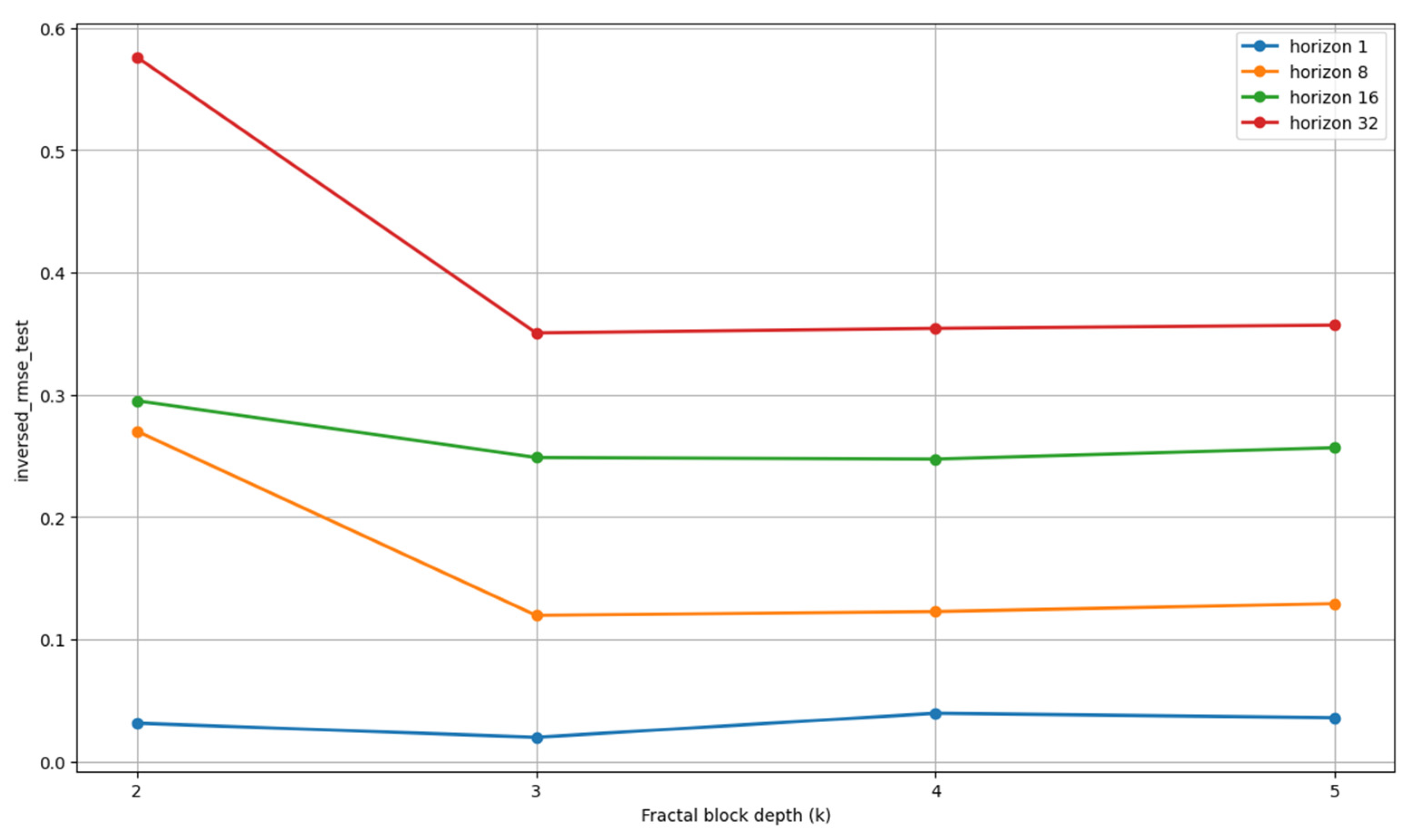
Thus, this reinforces the relevance of this solution not only in comparison to the classical FractalNet-LSTM but also as a reliable alternative to other neural network architectures. Furthermore, when comparing the results with Figure 2, we arrive at the important conclusion that branching into 3 branches performed better for shorter forecast horizons, while branching into 4 branches performed better for longer forecast intervals. A final strong argument in favor of the proposed solution is that all metrics showed the highest results for the same model. Therefore, this can be interpreted as stability and a clear advantage of the approach for this data. Summarizing the results, the best performance was achieved with a 1-step and 8-step forecast window, reaching R2 values of 0.9391 and 0.9195, respectively. At the same time, when forecasting 1 step ahead, the R2 increased by approximately 0.001 (from 0.9380 to 0.9391) relative to the classical approach, and when forecasting 8 steps ahead, the R2 increased by approximately 0.11 (from 0.8046 to 0.9195) relative to the classical approach.
The following results were obtained for the Green Energy Demand-Time Series Dataset. Here, the models also demonstrated good performance and high accuracy. Comparing the results on Table 3, we can see that fractal neural networks are the leaders here as well; they performed strongly over the short, medium, and long terms. Here, FractalNet-LSTM with a modified fractal block performed best with a 3-branch structure over the short- and medium-term periods. At the same time, for the long-term forecast, a 5-branch structure performed better. An important observation is that, just as in the previous data, a smaller number of branches is sufficient for shorter-term forecasts, while a longer-term forecast requires a higher number of branches. This shows that if the data has a fractal structure, increasing the number of branches allows for the capture of more complex features. Summarizing the results, the highest performance was observed in the 1-step and 8-step forecasts, reaching R2 values of 0.9808 and 0.8445, respectively. For 1-step forecasting, the R2 of the proposed architecture increased by approximately 0.05 (from 0.9316 to 0.9808) relative to the classical FractalNet-LSTM implementation, and for 8-step forecasting, the R2 increased by approximately 0.11 (from 0.7357 to 0.8445) relative to the classical implementation.
The final dataset considered was the Traffic Time Series Dataset. Analyzing the results in Table 4, we can conclude that fractal-based models did not consistently outperform CNN-LSTM. This can largely be explained by the fact that this dataset is characterized by strong fluctuations, which caused FractalNet-LSTM with a modified fractal block to perform worse than the alternatives.
For the same reason, CNN-LSTM was generally superior on this dataset, as it handles short-term fluctuations well. On the Traffic series the fractal-based models did not outperform CNN-LSTM, and at the longer horizons R2 became negative for all models; the proposed model retained an advantage only for the shortest horizon. This is consistent with the weak multifractal structure of the Traffic series reported in Section 3.1 and points to a boundary condition of the approach: the modified fractal block is beneficial mainly when self-similarity is accompanied by pronounced multifractality, rather than on near-monofractal, noise-dominated series.

3.3. Comparison of Model Accuracy for Different Branching Patterns in the Fractal Block

Here, we will examine how changing the number of branches affected the accuracy of the models. The results make it possible to identify branching configurations that were more effective for particular datasets and forecasting horizons. But the most interesting finding among these observations is that, in any case, the best results were obtained in models with more than two branches, which supports the relevance of treating the number of branches as a tunable architectural parameter.
Analysis of Figure 2 shows that the modification of the fractal block through parametric branching improves the forecasting performance for the Industrial Boiler Operations dataset compared with the classical two-branch FractalNet-LSTM configuration. The best results for shorter forecasting horizons were obtained with a three-branch structure, whereas further increasing the number of branches did not always lead to additional improvement and in some cases slightly reduced accuracy. However, as the forecasting horizon increases, configurations with a greater number of branches become more competitive, indicating that deeper or more complex fractal representations are more suitable for capturing long-term dependencies. This behavior can be explained by the pronounced fractal and multifractal properties of the Industrial Boiler time series, including a high DFA value and the widest multifractal spectrum among the analyzed datasets. Therefore, the obtained results support the main assumption of this study: for time series with strong self-similarity and heterogeneous scaling behavior, the architecture of the fractal block should be adapted to the complexity of the underlying temporal structure.
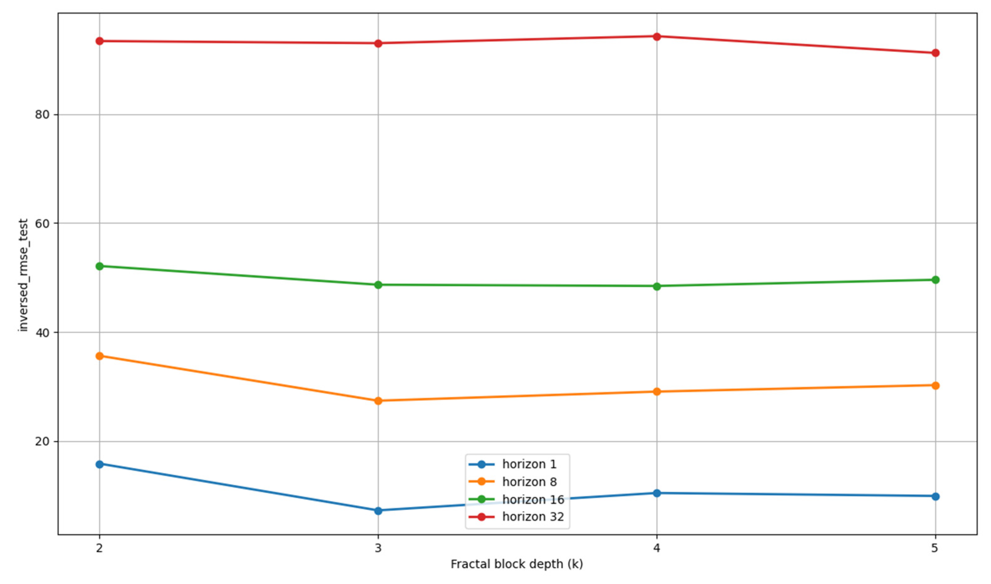
Figure 3 illustrates the influence of the branching configuration in the modified fractal block on the forecasting accuracy for the Green Energy Demand dataset. The obtained results show that the proposed parametric branching provides a clear advantage over the classical two-branch FractalNet-LSTM configuration, especially for short- and medium-term forecasting horizons. This confirms that the presence of self-similar properties in the data makes the use of fractal neural architectures methodologically justified.
At the same time, the improvement is less pronounced than for the Industrial Boiler Operations dataset, which can be explained by the more moderate multifractal characteristics of the Green Energy Demand series. Although the DFA value indicates the presence of scale-dependent behavior, the multifractal spectrum is narrower, suggesting a more homogeneous distribution of fluctuations across scales.
Consequently, increasing the number of branches improves the model’s ability to capture multiscale temporal dependencies, but excessive branching does not necessarily lead to proportional accuracy gains. These results support the assumption that the complexity of the fractal block should be selected according to both the degree of self-similarity and the strength of multifractal properties in the analyzed time series.
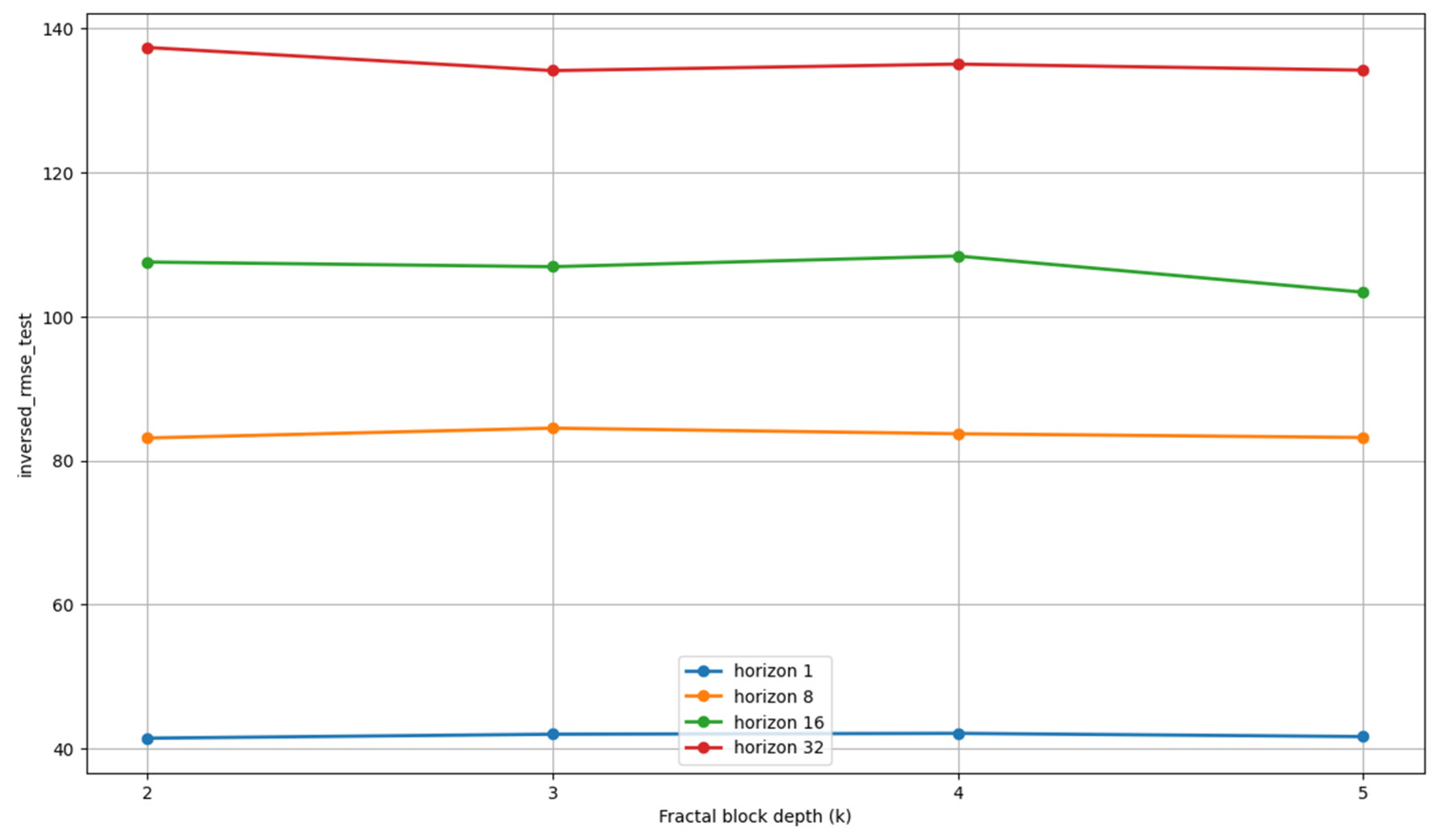
Figure 4 shows only limited and inconsistent improvements when the number of branches is increased. This can be attributed to the weaker multifractal properties of this series. Although the DFA results indicate the presence of self-similarity, the relatively narrow multifractal spectrum suggests that the scaling behavior of the traffic data is more homogeneous and closer to monofractal dynamics.
The less pronounced improvement of fractal-based models on the Traffic Time Series Dataset is likely associated with the weak multifractal structure of this series. While the data exhibit certain self-similar properties, the relatively lower multifractal measures indicate a limited degree of heterogeneous scaling behavior. Consequently, the advantages of the modified fractal block, which is designed to capture complex multiscale dependencies, become less evident than in datasets with stronger multifractality. However, the observed improvements for some branching configurations suggest that increasing the number of branches may still enhance the model’s ability to extract residual self-similar patterns, even when multifractal properties are weakly expressed.

4. Discussion

The results of this study demonstrate that the structural properties of time series should be explicitly considered when selecting and configuring forecasting models. The preliminary analysis based on DFA, Abry–Veitch, GPH, MF-DFA, and Wavelet Leaders methods showed that the investigated datasets exhibit different degrees of self-similarity, long-range dependence, and multifractality. These characteristics are important because they indicate that temporal dependencies may appear not only as local sequential patterns, but also as scale-dependent structures distributed across different time horizons. Therefore, the use of forecasting architectures capable of representing multiscale and hierarchical dependencies is methodologically justified for such data.
The obtained experimental results confirm that fractal neural networks are appropriate for forecasting time series with evident fractality and self-similarity. In particular, the proposed FractalNet-LSTM architecture with a modified fractal block demonstrated strong performance on the Industrial Boiler Operations and Green Energy Demand datasets, where fractal and multifractal properties were identified during the preliminary analysis. Compared with LSTM, BiLSTM, CNN-LSTM, and the classical FractalNet-LSTM, the modified architecture achieved better results across several forecasting horizons. This supports the assumption that the internal architecture of the forecasting model should reflect the intrinsic scale organization of the analyzed time series.
The advantage of the proposed approach can be explained by the ability of fractal neural networks to form several computational paths with different effective depths. Such a structure allows the model to simultaneously extract short-term local patterns and longer-term dependencies. This is especially relevant for self-similar time series, where similar structures may recur at different temporal scales. In this context, the modified fractal block functions as an embedded ensemble of paths with different representational capacities, while the aggregation of these paths enables the model to construct a more generalized multiscale representation of temporal dynamics.
An important finding of this study is that the classical two-branch fractal block is not always sufficient for time series with complex scale-dependent behavior. The introduction of parametric branching made it possible to adapt the fractal block to the complexity of the data. The experiments showed that models with more than two branches often outperformed the classical FractalNet-LSTM configuration. For shorter forecasting horizons, a smaller number of branches was usually sufficient, whereas longer horizons often benefited from a larger number of branches. This indicates that the branching complexity of the fractal block should be treated as a data-dependent architectural parameter rather than as a fixed design choice.
The results also suggest that the stronger the multifractal properties of a time series are, the more appropriate it becomes to use fractal neural networks with a deeper or more complex fractal block. Multifractality reflects heterogeneous scaling behavior, meaning that different fluctuation intensities may follow different scaling laws. In such cases, a shallow or weakly branched architecture may not be able to capture the full spectrum of temporal dependencies. A deeper fractal block, or a block with a larger number of branches, provides a richer set of computational paths and improves the ability of the model to approximate complex multiscale dynamics.
At the same time, the results obtained for the Traffic Time Series Dataset show that the presence of self-similarity alone does not guarantee the superiority of fractal architectures in all forecasting scenarios. Although this dataset demonstrated fractal characteristics, CNN-LSTM achieved competitive or better results for several horizons, which may be associated with strong local fluctuations and noise-like variations. This indicates that fractal neural networks are most effective when self-similarity is accompanied by sufficiently stable hierarchical or multifractal structure. However, because only three datasets were considered, the relationship between indicators such as Δh, Δα, Δζ, and the optimal number of branches cannot yet be formalized as a reliable quantitative rule. Therefore, future model selection should rely not only on a single self-similarity indicator, but on a comprehensive assessment of fractal and multifractal properties, including Δh, Δα, and Δζ.
The preprocessing procedure should also be considered when interpreting the results. In this study, the datasets were processed using a structurally consistent pipeline. Although the exact preprocessing operations depended on the original temporal resolution and quality of each dataset, the general procedure was kept uniform: missing values were handled where necessary, temporal resolution was adjusted when required, smoothing was applied to reduce high-frequency fluctuations. This ensures that the estimated fractal and multifractal indicators correspond to the same data representation that was used as input to the forecasting models.
The present study does not include a separate ablation analysis of preprocessing choices. Such an ablation would be important because smoothing, aggregation, and resampling may influence both the estimated scaling properties and the forecasting performance. A comprehensive preprocessing ablation would require comparing raw, smoothed, resampled, and combined preprocessing variants, followed by repeated fractal analysis and repeated model training for each variant. This is a broad and promising research direction, especially in the context of time-series forecasting for data with fractal and multifractal properties. Therefore, preprocessing ablation is considered a priority direction for future work.

5. Conclusions

This study confirms the relevance of using fractal neural networks for forecasting time series that exhibit fractality, self-similarity, and multiscale temporal dependencies. The proposed FractalNet-LSTM architecture with a modified fractal block improved forecasting accuracy compared with the classical two-branch FractalNet-LSTM and several non-fractal neural architectures. The main advantage of the proposed approach lies in its ability to adapt the branching structure of the fractal block and to represent temporal dependencies at different levels of abstraction.
The experimental results indicate that increasing the number of branches in the fractal block can improve forecasting performance, especially for datasets with more pronounced fractal or multifractal properties and for longer forecasting horizons. This suggests that the depth and branching complexity of the fractal block should be selected according to the structural properties of the time series. In particular, when multifractality is more significant, the use of deeper or more expressive fractal blocks becomes more justified, since such architectures are better suited to modeling heterogeneous scaling behavior.
Several limitations should be acknowledged. First, the reported metrics correspond to single training runs for each configuration; because the differences between the strongest models are in some cases small, a fuller evaluation using several random seeds, reported as the mean ± standard deviation together with a statistical significance test (for example, the Diebold–Mariano test), is required to confirm the robustness of the observed improvements. Second, the evaluation is based on three datasets, so the findings should be validated on a wider range of series before being generalised. Third, the baselines belong to the recurrent family (LSTM, BiLSTM, and CNN-LSTM); a comparison against convolutional, residual, and attention-based forecasters would provide a more complete assessment of the proposed architecture. Addressing these points is left for future work.
A priority area for future research is to establish a relationship between the depth or complexity of the branching of a fractal block and the multifractal characteristics of the time series. Future research should establish relationships between indicators such as Δh, Δα, and Δζ and hyperparameters responsible for the number of branches, recursive depth, and regularization parameters of the fractal block. Also, future experiments should be repeated over multiple random seeds and reported as mean ± standard deviation. This would allow the robustness of the proposed architecture to stochastic effects in the training process to be evaluated more rigorously.

Author Contributions

Conceptualization, N.S. and V.S.; methodology, N.S. and V.S.; software, A.M.; validation, A.M.; formal analysis, V.S. and A.M.; investigation, V.S. and A.M.; resources, A.M.; data curation, A.M.; writing—original draft preparation, V.S. and A.M.; writing—review and editing, N.S. and V.S.; visualization, A.M.; supervision, V.S.; project administration, N.S. All authors have read and agreed to the published version of the manuscript.

Funding

This research received no external funding.

Institutional Review Board Statement

Not applicable.

Informed Consent Statement

Not applicable.

Data Availability Statement

The data supporting the findings of this study are publicly available from Kaggle. The Traffic Time Series Dataset (available at: https://www.kaggle.com/datasets/stealthtechnologies/traffic-time-series-dataset, accessed on 1 July 2026)), the Green Energy Demand–Time Series Dataset (available at: https://www.kaggle.com/datasets/shivam131019/green-energy-demand-dataset, accessed on 1 July 2026), and the Time-Series of Industrial Boiler Operations (available at: https://www.kaggle.com/datasets/nikitamanaenkov/time-series-of-industrial-boiler-operations, accessed on 1 July 2026). No new datasets were generated during the study. All data were accessed in accordance with the respective platform’s terms of use.

Acknowledgments

In preparing this work, the authors used Grammarly v1.2.281.1928 for grammar and spelling checks. The authors have reviewed and edited the output and take full responsibility for the content of this publication.

Conflicts of Interest

The authors declare no conflicts of interest.

Abbreviations

The following abbreviations are used in this manuscript:
FractalNetFractal neural network
LSTMLong short-term memory
BiLSTMBidirectional long short-term memory
CNNConvolutional neural network
ARIMAAutoregressive integrated moving average
SARIMASeasonal autoregressive integrated moving average
ARCHAutoregressive conditional heteroskedasticity
GRUGated recurrent unit
RNNRecurrent neural network
TCNTemporal convolutional network
ResNetResidual neural network
Conv1DConvolutional one-dimensional layer
MSEMean squared error
MAEMean absolute error
RMSERoot mean square error
R 2 Coefficient of determination
ReLURectified Linear Unit
DFADetrended fluctuation analysis
GPHGeweke–Porter–Hudak
MF-DFAMultifractal Detrended Fluctuation Analysis

References

  1. Hyndman, R.J.; Athanasopoulos, G. Forecasting: Principles and Practice, 2nd ed.; OTEXTS: Melbourne, Australia, 2018. [Google Scholar]
  2. Box, G.E.P.; Jenkins, G.M.; Reinsel, G.C.; Ljung, G.M. Time Series Analysis: Forecasting and Control, 5th ed.; In Wiley Series in Probability and Statistics; John Wiley & Sons, Inc.: Hoboken, NJ, USA, 2016. [Google Scholar]
  3. Chatfield, C. The Analysis of Time Series: An Introduction, 6th ed.; Chapman & Hall/CRC: Boca Raton, FL, USA, 2004. [Google Scholar]
  4. Hamilton, J.D. Time Series Analysis; Princeton University Press: Princeton, NJ, USA, 1994. [Google Scholar]
  5. Kolemen, E.; Egrioglu, E.; Bas, E.; Turkmen, M. A new deep recurrent hybrid artificial neural network of gated recurrent units and simple seasonal exponential smoothing. Granul. Comput. 2024, 9, 7. [Google Scholar] [CrossRef] [Scilit]
  6. Kirichenko, L.; Koval, Y.; Yakovlev, S.; Chumachenko, D. Anomaly Detection in Fractal Time Series with LSTM Autoencoders. Mathematics 2024, 12, 3079. [Google Scholar] [CrossRef] [Scilit]
  7. Shymanskyi, V.; Sabov, V. An RNN-Based Stock Price Forecasting Model Enhanced by Sentiment Analysis of the Daily Financial News. In Advances in Computer Science for Engineering and Education VII; Lecture Notes on Data Engineering and Communications Technologies; Hu, Z., Yanovsky, F., Dychka, I., He, M., Eds.; Springer Nature: Cham, Switzerland, 2025; Volume 242, pp. 261–270. [Google Scholar] [CrossRef] [Scilit]
  8. Kaminsky, R.; Mochurad, L.; Shakhovska, N.; Melnykova, N. Calculation of the Exact Value of the Fractal Dimension in the Time Series for the Box-Counting Method. In Proceedings of the 2019 9th International Conference on Advanced Computer Information Technologies (ACIT); IEEE: Ceske Budejovice, Czech Republic, 2019; pp. 248–251. [Google Scholar] [CrossRef] [Scilit]
  9. Kirkby, M.J. The fractal geometry of nature. Benoit B. Mandelbrot. W. H. Freeman and co., San Francisco, 1982. No. of pages: 460. Price: £22.75 (hardback). Earth Surf. Process. Landf. 1983, 8, 406. [Google Scholar] [CrossRef] [Scilit]
  10. Larsson, G.; Maire, M.; Shakhnarovich, G. FractalNet: Ultra-Deep Neural Networks without Residuals. arXiv 2017, arXiv:1605.07648. [Google Scholar] [CrossRef] [Scilit]
  11. Baicoianu, A.; Gavrilă, C.G.; Pacurar, C.M.; Pacurar, V.D. Fractal interpolation in the context of prediction accuracy optimization. arXiv 2024, arXiv:2403.00403. [Google Scholar] [CrossRef] [Scilit]
  12. Shymanskyi, V.; Ratinskiy, O.; Shakhovska, N. Fractal Neural Network Approach for Analyzing Satellite Images. Appl. Artif. Intell. 2025, 39, 2440839. [Google Scholar] [CrossRef] [Scilit]
  13. Lara-Benítez, P.; Carranza-García, M.; Luna-Romera, J.M.; Riquelme, J.C. Temporal Convolutional Networks Applied to Energy-Related Time Series Forecasting. Appl. Sci. 2020, 10, 2322. [Google Scholar] [CrossRef] [Scilit]
  14. Lim, B.; Zohren, S. Time-series forecasting with deep learning: A survey. Philos. Trans. R. Soc. Math. Phys. Eng. Sci. 2021, 379, 20200209. [Google Scholar] [CrossRef] [Scilit] [PubMed]
  15. Benidis, K.; Rangapuram, S.S.; Flunkert, V.; Wang, Y.; Maddix, D.; Turkmen, C.; Gasthaus, J.; Bohlke-Schneider, M.; Salinas, D.; Stella, L.; et al. Deep Learning for Time Series Forecasting: Tutorial and Literature Survey. ACM Comput. Surv. 2023, 55, 1–36. [Google Scholar] [CrossRef] [Scilit]
  16. Song, X.; Deng, L.; Wang, H.; Zhang, Y.; He, Y.; Cao, W. Deep learning-based time series forecasting. Artif. Intell. Rev. 2024, 58, 23. [Google Scholar] [CrossRef] [Scilit]
  17. Zhou, H.; Zhang, S.; Peng, J.; Zhang, S.; Li, J.; Xiong, H.; Zhang, W. Informer: Beyond Efficient Transformer for Long Sequence Time-Series Forecasting. Proc. AAAI Conf. Artif. Intell. 2021, 35, 11106–11115. [Google Scholar] [CrossRef] [Scilit]
  18. Wu, H.; Xu, J.; Wang, J.; Long, M. Autoformer: Decomposition Transformers with Auto-Correlation for Long-Term Series Forecasting. arXiv 2021, arXiv:2106.13008. [Google Scholar] [CrossRef] [Scilit]
  19. Nie, Y.; Nguyen, N.H.; Sinthong, P.; Kalagnanam, J. A Time Series is Worth 64 Words: Long-term Forecasting with Transformers. arXiv 2022, arXiv:2211.14730. [Google Scholar] [CrossRef] [Scilit]
  20. Zhang, G.; Patuwo, B.E.; Hu, M.Y. Forecasting with artificial neural networks. Int. J. Forecast. 1998, 14, 35–62. [Google Scholar] [CrossRef] [Scilit]
  21. Casolaro, A.; Capone, V.; Iannuzzo, G.; Camastra, F. Deep Learning for Time Series Forecasting: Advances and Open Problems. Information 2023, 14, 598. [Google Scholar] [CrossRef] [Scilit]
  22. Shakhovska, N.; Shymanskyi, V.; Prymachenko, M. FractalNet-LSTM Model for Time Series Forecasting. Comput. Mater. Contin. 2025, 82, 4469–4484. [Google Scholar] [CrossRef] [Scilit]
  23. Peng, C.-K.; Buldyrev, S.V.; Havlin, S.; Simons, M.; Stanley, H.E.; Goldberger, A.L. Mosaic organization of DNA nucleotides. Phys. Rev. E 1994, 49, 1685–1689. [Google Scholar] [CrossRef] [Scilit] [PubMed]
  24. Kantelhardt, J.W.; Zschiegner, S.A.; Koscielny-Bunde, E.; Havlin, S.; Bunde, A.; Stanley, H.E. Multifractal detrended fluctuation analysis of nonstationary time series. Phys. Stat. Mech. Its Appl. 2002, 316, 87–114. [Google Scholar] [CrossRef] [Scilit]
  25. Mallat, S.G. A Wavelet Tour of Signal Processing: The Sparse Way, 3rd ed.; Elsevier: Amsterdam, The Netherlands; Academic Press: Boston, MA, USA, 2009. [Google Scholar]
  26. Geweke, J.; Porter-Hudak, S. The estimation and application of long memory time series models. J. Time Ser. Anal. 1983, 4, 221–238. [Google Scholar] [CrossRef] [Scilit]
  27. Jaffard, S.; Lashermes, B.; Abry, P. Wavelet Leaders in Multifractal Analysis. In Wavelet Analysis and Applications; Qian, T., Vai, M.I., Xu, Y., Eds.; Birkhäuser: Basel, Switzerland, 2007; pp. 201–246. [Google Scholar]
  28. Time-Series of Industrial Boiler. Available online: https://www.kaggle.com/datasets/nikitamanaenkov/time-series-of-industrial-boiler-operations (accessed on 1 July 2026).
  29. Green Energy Demand—Time Series Dataset. Available online: https://www.kaggle.com/datasets/shivam131019/green-energy-demand-dataset (accessed on 1 July 2026).
  30. Traffic Time Series Dataset. Available online: https://www.kaggle.com/datasets/stealthtechnologies/traffic-time-series-dataset (accessed on 1 July 2026).
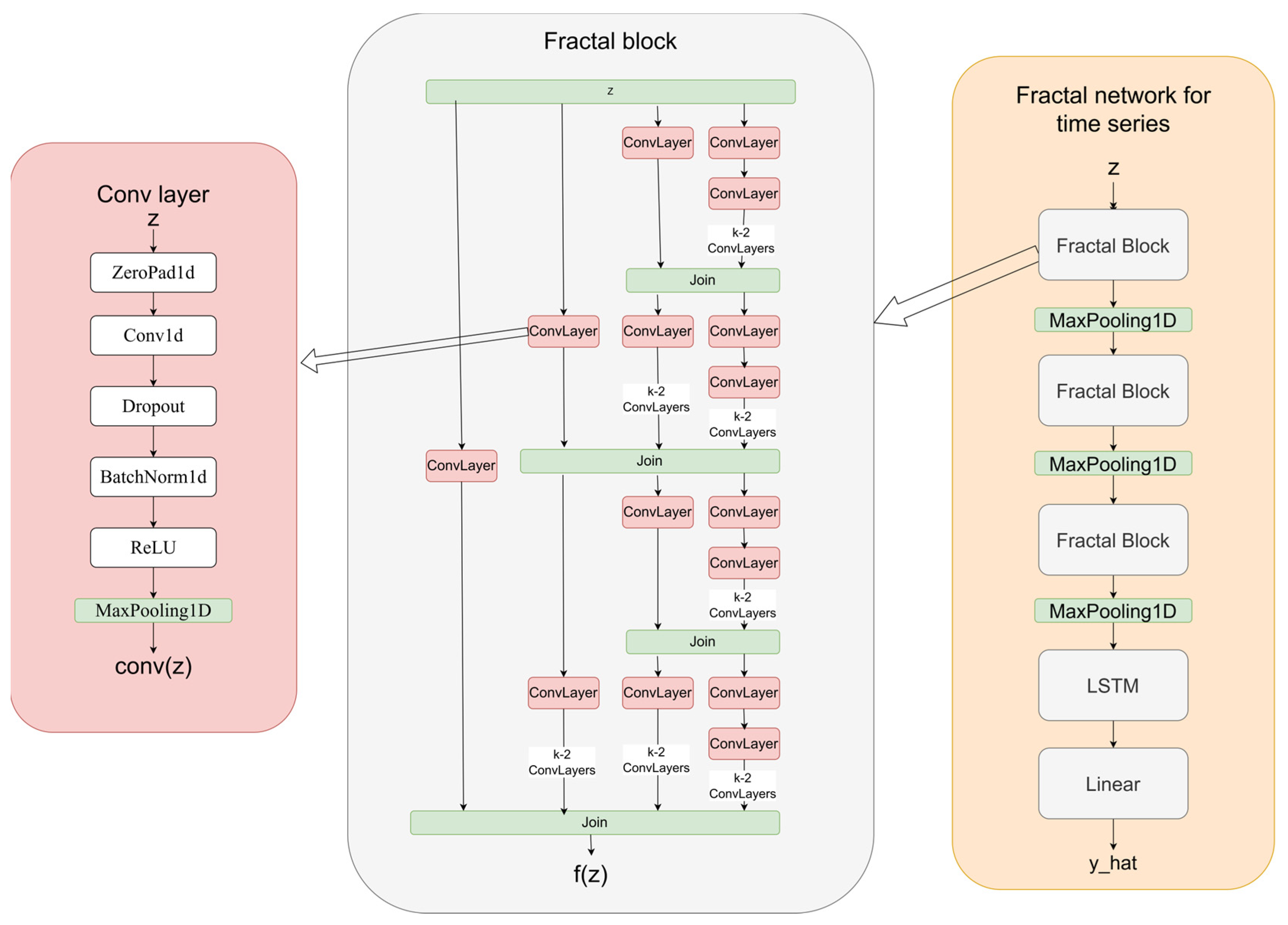
Figure 1. FractalNet-LSTM architecture with a modified fractal block.
Applsci 16 07563 g001
Figure 2. Forecasting accuracy of FractalNet-LSTM models with 2, 3, 4, and 5 branches for the Industrial Boiler Operations dataset.
Applsci 16 07563 g002
Figure 3. Forecasting accuracy of FractalNet-LSTM models with 2, 3, 4, and 5 branches for the Green Energy Demand dataset.
Applsci 16 07563 g003
Figure 4. Forecasting accuracy of FractalNet-LSTM models with 2, 3, 4, and 5 branches for the Traffic Time Series Dataset.
Applsci 16 07563 g004
Table 1. Summary estimates of self-similarity and fractality indicators of time series.
Method (Indicator)Green Energy
Demand
Industrial BoilerTraffic
DFA (α)1.2240.8320.897
DFA (H) (fGn, fBm)0.224 (fBm)0.832 (fGn)0.897 (fGn)
Abry–Veitch (H)0.4870.3780.150
GPH (d)1.7311.1461.281
MF-DFA (Δh)0.310.6570.215
MF-DFA (Δα)0.570.8320.383
WL (Δζ)2.8574.0043.633
Process typeMultifractal, antipersistentMultifractal,
persistent
Weak multifractal, persistent
Table 2. Comparative test results of trained models on the Industrial Boiler Operations dataset.
OutputModelMAEMAPE R 2 RMSE
1bilstm0.14860.00030.89330.1623
cnn-lstm0.17830.00030.85760.1969
fractalnet0.02755.09 × 10−50.93800.0313
fractalnet k30.01703.13 × 10−50.93910.0198
fractalnet k40.03576.59 × 10−50.93830.0394
fractalnet k50.03266.02 × 10−50.93790.0358
lstm0.14970.00030.89310.1635
8bilstm0.38640.00070.57280.4325
cnn-lstm0.30450.00060.69790.3496
fractalnet0.22750.00040.80460.2701
fractalnet k30.09600.00020.91950.1195
fractalnet k40.09880.00020.91720.1226
fractalnet k50.10470.00020.91010.1291
lstm0.23500.00040.67760.2759
16bilstm0.30340.00060.57360.3682
cnn-lstm0.26800.00040.67510.3360
fractalnet0.23260.00040.76470.2950
fractalnet k30.20070.00040.82090.2486
fractalnet k40.19950.00040.82650.2473
fractalnet k50.20590.00040.81060.2566
lstm0.31080.00060.54720.3752
32bilstm0.95260.0018−2.12101.1040
cnn-lstm0.52480.0010−0.21130.6567
fractalnet0.44910.0008−0.00190.5761
fractalnet k30.26150.00050.55360.3505
fractalnet k40.26030.00040.56100.3542
fractalnet k50.26800.00050.55560.3568
lstm0.95020.0018−2.12561.0993
Table 3. Comparative test results of trained models on the Green Energy Demand-Time Series Dataset.
OutputModelMAEMAPE R 2 RMSE
1bilstm15.56280.00750.928718.9401
cnn-lstm42.07430.01960.296647.0445
fractalnet13.41610.00570.931615.8199
fractalnet k35.74670.00230.98087.2386
fractalnet k48.39700.00330.956710.4270
fractalnet k58.07600.00330.96539.8890
lstm15.25780.00740.930118.6222
8bilstm39.44630.01910.488649.5381
cnn-lstm34.98830.01540.572043.6789
fractalnet27.46780.01250.735735.6145
fractalnet k321.04440.00950.844527.3641
fractalnet k422.57170.01010.820029.0351
fractalnet k523.62890.01050.803430.2219
lstm39.16360.01900.491149.3450
16bilstm46.73670.0228−0.015160.4589
cnn-lstm45.08400.02060.283558.1579
fractalnet38.44760.01800.444852.0909
fractalnet k336.47010.01710.511848.6529
fractalnet k436.36510.01710.508248.4262
fractalnet k537.58600.01760.486249.5563
lstm59.17040.0288−0.238375.2114
32bilstm86.28400.0410−2.1379109.7214
cnn-lstm84.53190.0394−1.6826107.0107
fractalnet69.39450.0331−0.932893.3762
fractalnet k370.08090.0333−0.916992.9875
fractalnet k471.44350.0337−0.978794.2734
fractalnet k568.88950.0329−0.850791.2031
lstm90.87080.0427−2.3025113.8390
Table 4. Comparative test results of trained models on the Traffic Time Series Dataset.
OutputModelMAEMAPE R 2 RMSE
1bilstm26.0800.0210.84341.038
cnn-lstm26.8540.0220.83642.141
fractalnet26.4360.0220.84241.447
fractalnet k325.8620.0210.85542.001
fractalnet k426.1220.0220.83742.121
fractalnet k525.6030.0210.85541.670
lstm27.2590.0220.83641.860
8bilstm64.5290.0530.41485.253
cnn-lstm61.7260.0500.46181.671
fractalnet62.6850.0510.45083.146
fractalnet k362.7060.0510.46084.516
fractalnet k463.4990.0520.45583.735
fractalnet k562.9820.0510.45683.213
lstm64.8600.0530.40985.145
16bilstm90.7040.074−0.049116.399
cnn-lstm81.1510.0660.132103.901
fractalnet83.6320.0680.079107.587
fractalnet k383.2600.0680.088106.937
fractalnet k483.6670.0680.065108.419
fractalnet k580.4820.0650.066103.396
lstm88.7350.073−0.048112.970
32bilstm112.5780.092−0.588138.893
cnn-lstm106.5620.087−0.450132.131
fractalnet110.4770.091−0.634137.392
fractalnet k3108.0940.088−0.455134.178
fractalnet k4109.0990.090−0.604135.081
fractalnet k5107.8010.088−0.533134.238
lstm113.3080.093−0.637138.858
Disclaimer/Publisher’s Note: The statements, opinions and data contained in all publications are solely those of the individual author(s) and contributor(s) and not of MDPI and/or the editor(s). MDPI and/or the editor(s) disclaim responsibility for any injury to people or property resulting from any ideas, methods, instructions or products referred to in the content.