Explainable Susceptibility Modelling of Urban Ground Collapse Considering Dynamic Rainfall and Background Controls: A Case Study in Shenzhen, China

Abstract

Urban ground collapse (UGC) threatens dense coastal cities because failures can occur abruptly beneath roads and buried lifelines. We developed a dynamic and interpretable machine-learning framework for UGC susceptibility assessment in Shenzhen, China. We integrated 1687 events from 2017 to 2024 with 20 predictors covering terrain, rainfall, drainage infrastructure and urban disturbance. Event-date rainfall was assigned to collapse samples, and background controls received year-constrained pseudo-event dates after spatial exclusion. Three tree-ensemble models were evaluated under random 75/25 testing, leave-one-district-out spatial validation and temporal hold-out testing. The selected LightGBM 1:5 model achieved ROC-AUC = 0.934, AP = 0.790 and BA = 0.860 in random testing, with more conservative ROC-AUC values of 0.905 and 0.884 under spatial and temporal validation. High-rainfall mapping expanded high and very high susceptibility zones from 4.60% to 15.26% and increased event capture from 19.32% to 58.92%. Grouped SHAP indicated comparable pipeline and rainfall contributions (26.01% and 25.13%). The leading predictors were pipe burial depth, road density and 30-day rainfall. PDP and spatial SHAP diagnostics highlighted high model responses where deep pipes coincided with high antecedent rainfall or dense roads in mature urban cores. This framework supports the rainfall-conditioned, mechanism-informed susceptibility diagnosis for early warning and mitigation.

1. Introduction

Low-lying coastal cities with heterogeneous and compressible deposits host some of the fastest-growing high-density urban centers globally [1,2]. Rapid urbanization and climate warming are increasing the exposure of these cities to more frequent and intense hazards, including compound flooding, land subsidence, and localized ground collapse [3,4]. Urban ground collapse (UGC) is particularly disruptive because it occurs abruptly, affects roads and buried lifelines, and can trigger cascading impacts on public-safety and transport consequences in densely built environments [5]. Characterizing the spatial and temporal patterns of UGC, identifying conditions associated with failure, and developing interpretable susceptibility models are therefore essential for risk-informed urban management.

In high-density urban environments, UGC should not be viewed solely through the lens of natural karst collapse or rainfall-induced slope failure [6]. Rather, it commonly emerges from interactions between natural controls, including intense rainfall, shallow groundwater and sensitive Quaternary deposits, and anthropogenic disturbances, such as pipe leakage, trench backfill, road construction and underground engineering. Roadworks can disturb pavement layers and trench backfill, whereas pipe installation and dense underground utility networks can introduce preferential flow paths, structural defects, and leakage interfaces [7,8,9]. Failures are more likely where road works, pipe leakage, susceptible geological conditions, and dense underground utility networks interact [10,11]. Excavation, tunnelling, and building construction may also leave latent loosened zones that become active only under antecedent wetness, groundwater fluctuation, or repeated loading [12,13]. These disturbances can create weak zones and preferential routes for water and sediment migration [12,14], supporting the interpretation of UGC as a coupled soil–water–infrastructure failure process [15].

Such coupled processes exhibit nonlinear and threshold-sensitive responses, motivating the use of data-driven susceptibility modelling [16]. A short rainfall event may produce no visible damage where buried utilities and backfill remain intact [17,18,19]. The same event may contribute to collapse where ageing pipes and poorly compacted trench backfill coincide with surface conditions that concentrate runoff and increase local hydraulic loading, such as impermeable pavement or local depressions [20,21,22]. In many susceptibility assessments, rainfall is still represented as a long-term climatic layer or a static conditioning factor, limiting the distinction between baseline spatial vulnerability and rainfall-associated susceptibility change [23,24]. Dynamic landslide studies have addressed this temporal dimension by combining susceptibility maps with rainfall thresholds or event-based accumulation windows [25]. Accordingly, a dynamic UGC framework should represent rainfall not only as a background climatic attribute but also as event-specific forcing [8,25]. However, these frameworks are predominantly designed for slope-controlled failures and do not explicitly represent the road-pipe systems and underground engineering that mediate UGC. A UGC-specific framework therefore needs to separate static urban predisposition from event-aligned rainfall forcing within a common sampling design.

Machine-learning algorithms offer a practical means of modelling these conditional dependencies because they can accommodate nonlinear thresholds, high-dimensional heterogeneity and interactions among heterogeneous spatial layers [26,27]. In geohazard susceptibility studies, tree-based ensemble models have been widely used to integrate terrain, hydrological, geological and anthropogenic predictors, and recent urban road-collapse studies have further shown their potential for fine-scale urban geohazard assessment [16,28]. However, high predictive scores alone do not ensure that a susceptibility model is physically interpretable or geotechnically credible [29,30]. Black-box classifiers may reproduce the spatial pattern of reported events rather than the process associated with collapse occurrence [31,32,33]. This concern is particularly relevant to UGC inventories because reported events often occur along roads, construction corridors, and heavily monitored districts [7,28,34].

Geospatial model performance is highly sensitive to the way training and testing samples are separated. Neighbouring grid cells may also share similar geology, rainfall, drainage networks, and reporting conditions, so random validation can overstate model skill when spatially similar samples are split between training and testing sets [35,36,37]. However, many existing applications remain dominated by static conditioning layers and conventional random or pseudo-absence sampling. If background controls are drawn from urban settings that differ systematically from recorded collapse locations, the classifier may learn broad contrasts in urbanization, infrastructure availability or reporting intensity rather than collapse-related conditions [29,38,39]. Therefore, a methodologically credible UGC framework should construct controls from plausible built-up ground, exclude immediate recorded-event neighbourhoods, assign temporally comparable rainfall histories, and evaluate generalization under spatially and temporally separated validation designs.

Explainable artificial intelligence provides a way to examine whether high-performing models are consistent with plausible hydro-infrastructure mechanisms [31]. SHAP decomposes each prediction into additive feature contributions at global and local scales [40]. Partial dependence plots (PDPs) summarise average model responses, whereas individual conditional expectation (ICE) curves show sample-specific responses [41]. Together, these tools help characterize nonlinear model behaviors and interactions in high-performing models [31,32]. For example, a high SHAP contribution from road-related predictors indicates that the fitted model relies strongly on the road-corridor signal. This pattern may be consistent with traffic loading, utility density, trench disturbance, drainage concentration, or reporting intensity [31,32]. Spatial SHAP mapping and GeoDetector can further examine whether explanation values are organized by district, terrain, infrastructure, or other spatial strata [42,43]. Recent geohazard studies emphasize the need to move from event-level prediction to spatially regional interpretation [44]. For the UGC, knowing that a variable is globally important is insufficient for operational interpretation because the meaning of pipe burial depth, road density or engineering proximity may vary among districts and under different rainfall states. The spatially organized model-behaviour diagnostics provide a structured basis for comparing statistical predictions with geotechnical interpretation.

To address these gaps, this study develops a dynamic, spatiotemporally constrained and spatially explainable machine-learning framework for UGC susceptibility assessment in Shenzhen. The framework is designed to answer three questions: how rainfall is associated with changes in predicted city-scale collapse susceptibility, how underground drainage infrastructure and road-corridor disturbance are related to this modelled response, and how model-inferred explanatory patterns vary across urban districts. Specifically, we (1) construct a mechanism-informed database by integrating 1687 collapse events from 2017 to 2024 with 20 geo-topographic, hydrological, rainfall, drainage-infrastructure and urban-disturbance predictors; (2) assign event-specific rainfall to collapse samples and year-constrained pseudo-event dates to background controls sampled within a multi-source built-up domain; (3) compare Random Forest, XGBoost, and LightGBM under multiple collapse-to-control ratios and evaluate the selected model using random hold-out, leave-one-district-out spatial, and forward temporal hold-out validation; and (4) interpret the selected model using SHAP, spatial SHAP diagnostics and PDP-based response analysis. The contribution is therefore not only a susceptibility map, but a reproducible strategy for combining dynamic rainfall assignment, underground-infrastructure interpretation and mechanism-informed urban mitigation.

2. Materials and Methods

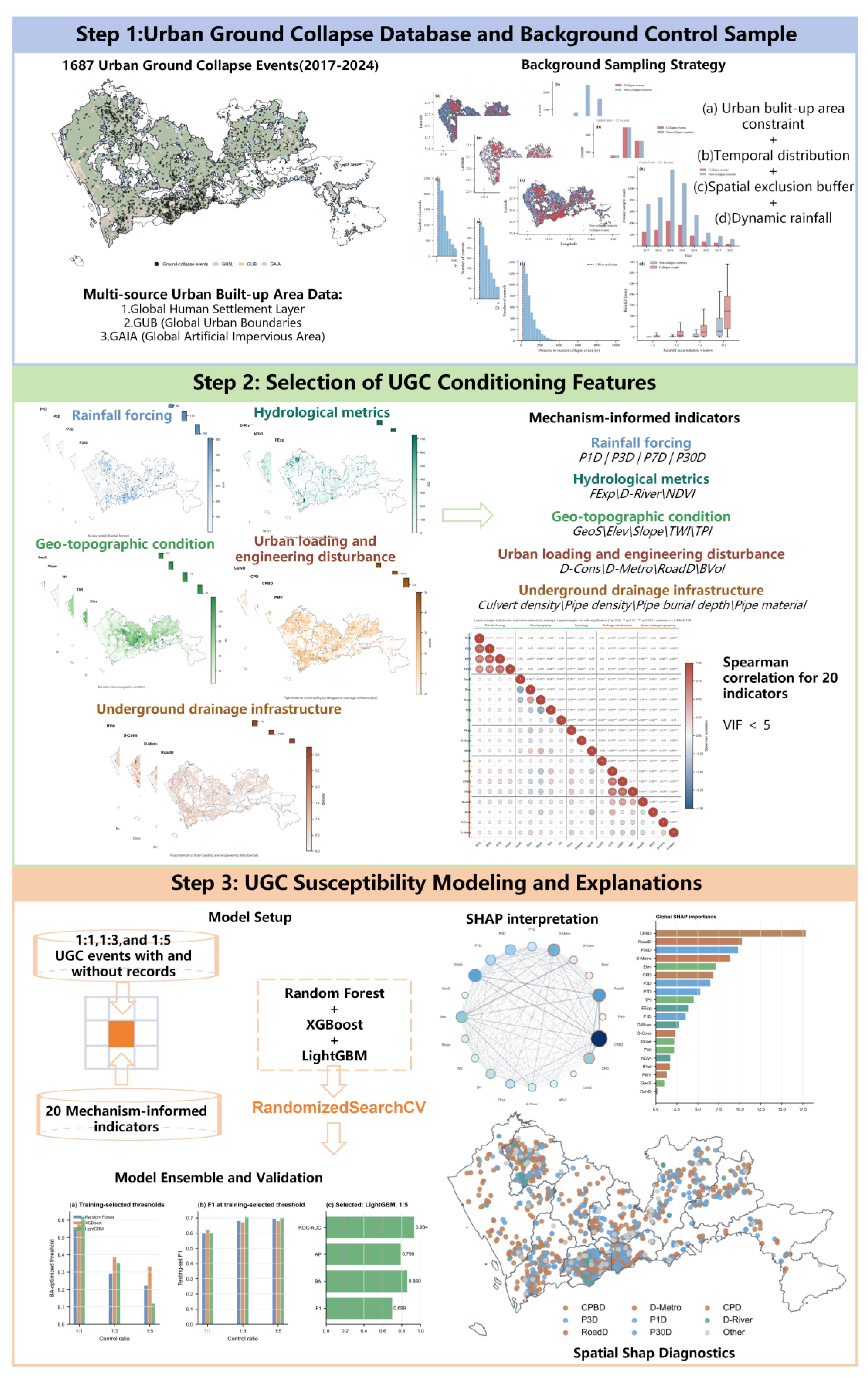
The methodological workflow was designed to develop and evaluate a dynamic susceptibility model that can be interpreted in relation to plausible UGC mechanisms. As shown in Figure 1, the workflow consisted of three steps. First, recorded UGC events were cleaned, spatially matched to the built-up modelling domain, and paired with spatiotemporally constrained background controls generated through reverse sampling. Second, 20 mechanism-informed predictors were prepared to represent geo-topographic conditions, hydrological settings, rainfall forcing, underground drainage infrastructure, road-corridor loading, and engineering disturbance. Third, Random Forest, XGBoost, and LightGBM were trained and validated under three collapse-to-background ratios to identify a robust city-level susceptibility model. Within this final stage, the selected model was applied to rainfall-scenario mapping and interpreted using SHAP, spatial SHAP diagnostics, PDP-ICE, and two-dimensional PDP surfaces to examine dominant contributors, nonlinear response patterns, and district-level spatial heterogeneity.

2.1. Study Area and UGC Inventory

Shenzhen has experienced frequent UGC incidents in recent years and provides a representative case for assessing collapse susceptibility in a rapidly urbanized coastal megacity. The city combines high-density vertical development, intensive underground-space utilization, extensive buried lifelines, and hydrogeological complexity.

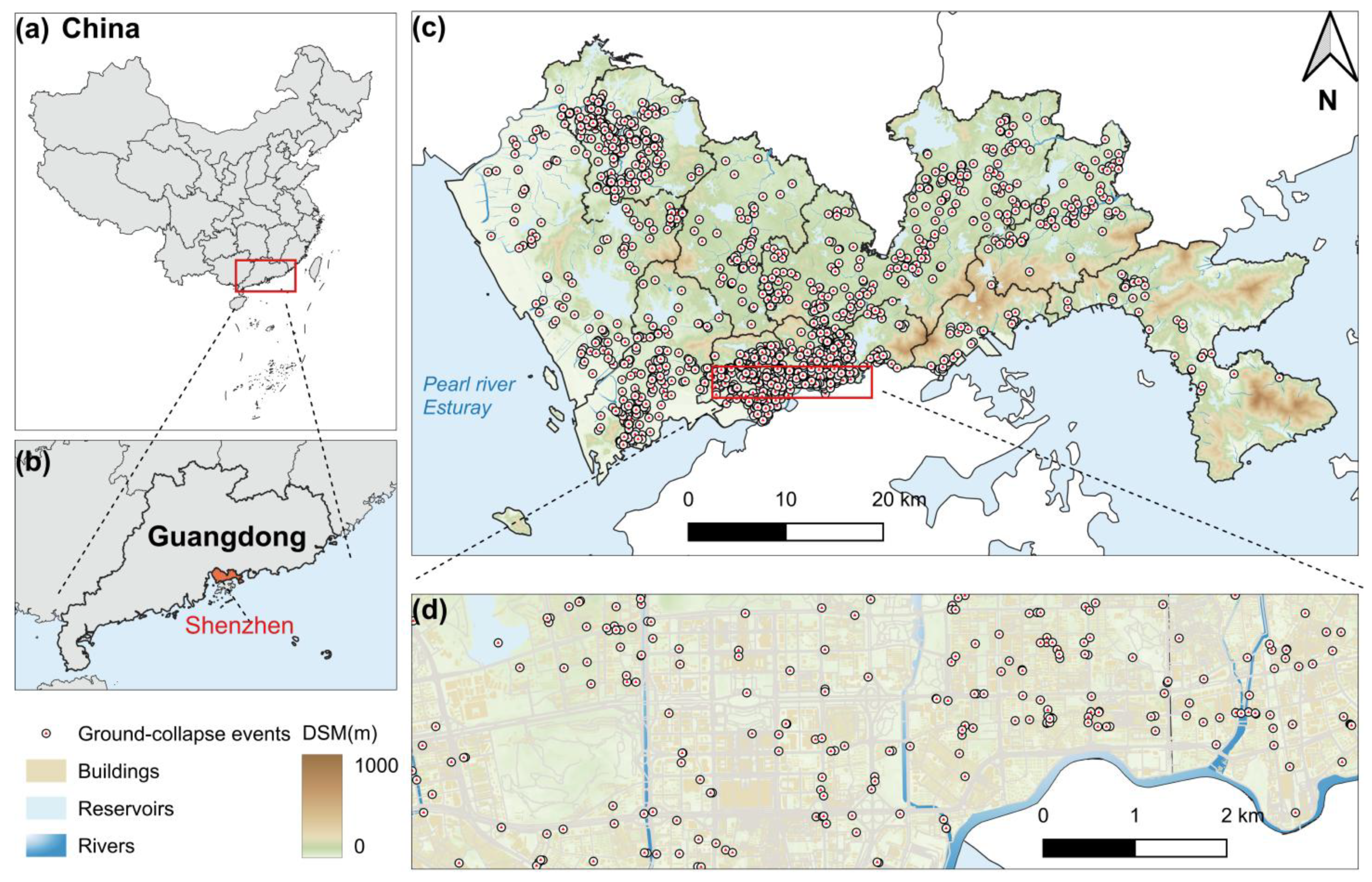
Observed collapse records were obtained from the Ground Collapse Prevention and Control Office of the Shenzhen Municipal Bureau of Planning and Natural Resources (Figure 2). The inventory represents actual reported incidents and includes the reported longitude, latitude and occurrence date of each event, as submitted by sub-district officers through the municipal reporting system. Records with valid coordinates and event dates were retained. Duplicate entries with identical spatial and temporal attributes were removed to reduce repeated reporting. The event coordinates were treated as reported incident locations rather than exact surveyed cavity boundaries (Figure 3).

Although recorded events are distributed across the city, their occurrence is spatially heterogeneous, with clear differences among administrative districts (Figure 2). Shenzhen’s low-lying built-up areas are characterized by dense road corridors, extensive metro infrastructure, and intensive building development; seasonal rainfall and short-duration storms can impose additional hydraulic loading on drainage and subsurface infrastructure systems.

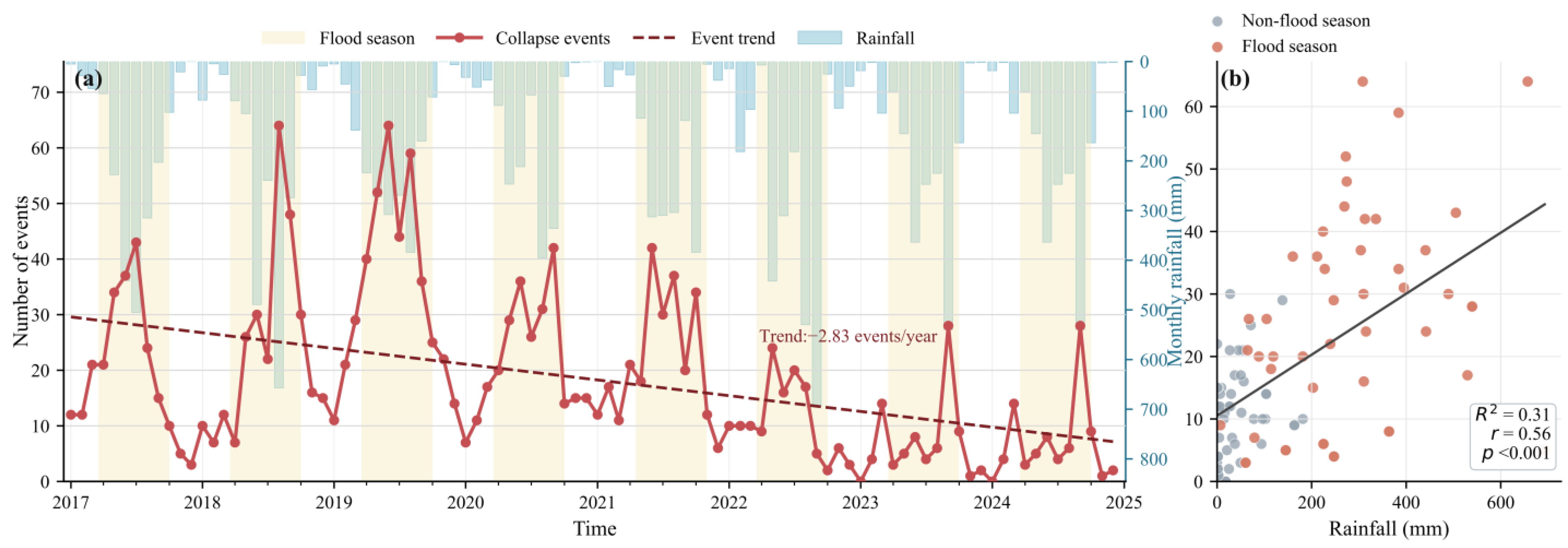
The temporal distribution of collapse events shows a clear seasonal association with precipitation: flood-season months accounted for 87.0% of total rainfall and 69.7% of collapse incidents, and monthly collapse counts were positively correlated with monthly rainfall (Pearson’s r = 0.56, p < 0.001). This temporal association supports the inclusion of antecedent rainfall as a dynamic predictor. However, rainfall is interpreted here as a potential trigger superimposed on spatially variable subsurface vulnerability, rather than as a stand-alone cause of collapse.

2.2. Mechanism-Informed Predictors

To represent the coupled geo-environmental and anthropogenic interactions associated with UGC, the study used 20 indicators (

Table 1. Summary of the indicators used in the study.

Category	Full Indicator Name	Suggested Abbreviation	Meaning	References
Geo-topographic condition	Engineering-geological susceptibility score	GeoS	Engineering-geological type-based collapse-proneness score (Supplementary Table S1)	[45,46]
	Elevation	Elev	Mean elevation of grid	[47]
	Slope	Slope	Terrain slope	[48]
	Topographic wetness index	TWI	Potential water accumulation condition	[49]
	Topographic position index	TPI	Local relative terrain position	[49]
Hydrological metrics	Flood exposure area	FExp	Grid exposure to simulated inundation area	[50,51]
	River distance	D-River	Distance to river	[43,47]
	NDVI	NDVI	Vegetation/land-cover condition	[49]
Rainfall forcing	1-day rainfall	P1D	Event-day rainfall	[11,52]
	3-day rainfall	P3D	Antecedent 3-day accumulated rainfall	[11]
	7-day rainfall	P7D	Antecedent 7-day accumulated rainfall	[52]
	30-day rainfall	P30D	Antecedent 30-day accumulated rainfall	[11]
Underground drainage infrastructure	Culvert density	CulvD	Culvert and underground channel density	[53]
	Pipe density	CPD	Major drainage pipeline length density	[54]
	Pipe burial depth	CPBD	Mean burial depth of major drainage pipelines	[55,56]
	Pipe material	PMV	Vulnerability score inferred from pipe material (Supplementary Table S2)	[57]
Urban loading and engineering disturbance	Construction distance	D-Cons	Distance to construction sites or engineering targets	[58]
	Metro distance	D-Metro	Distance to metro lines	[59]
	Road density	RoadD	Road-network density in grid	[43]
	Building volume	BVol	Building volume or development intensity proxy	[46]

), organized into five process groups: geo-topographic conditions, hydrological and flood environments, rainfall forcing, underground drainage infrastructure, and urban loading and engineering disturbance. Geological and terrain indicators characterize material and terrain conditions relevant to saturation, seepage, and potential cavity development. Hydrological and flood variables describe potential water accumulation and river proximity. Rainfall metrics represent both event-scale and antecedent hydrological forcing. Infrastructure and urban-disturbance variables, including road density, pipeline density, pipe burial depth, metro proximity, construction distance, and building volume, represent engineered conditions that may alter stress, seepage, and backfill stability.

A 30 m grid was selected as the basic modelling unit to balance the spatial scale of UGC-related processes, positional uncertainty in the reported inventory, source-data resolution and computational feasibility. The grid was intended to represent the local urban context of susceptibility—including road corridors, drainage-pipeline segments, trench-backfill zones, terrain conditions, and nearby engineering disturbances—rather than the exact boundary of an individual cavity or surface opening. Although the final surface opening of a collapse may be smaller than 30 m, the relevant predisposing environment is commonly organized along road and utility corridors at scales of tens of meters. Moreover, many collapse records represent reported incident locations rather than surveyed cavity boundaries; therefore, a much finer grid could introduce pseudo-precision and spatial noise. Several source datasets, including terrain, digital surface model, and built-up-area products, are also available at or can be robustly harmonized to approximately 30 m. For the 1234.14 km² built-up modelling domain, a 30 m grid contains approximately 1.37 million cells, whereas a 10 m grid would contain approximately 12.34 million cells and a 1 m grid would exceed 1.23 billion cells. The 30 m resolution was therefore considered appropriate for city-scale UGC susceptibility modelling.

For grid cells not intersected by drainage pipelines, pipe-density variables were assigned zero, whereas burial-depth and pipe-material attributes were assigned a predefined no-pipeline category. This avoided interpreting the absence of a pipeline as shallow burial depth or low material vulnerability. Pairwise Spearman correlation coefficients and variance inflation factors (VIFs) were examined to identify severe predictor redundancy. All retained predictors had VIF values below 5, and the complete diagnostic results are provided in Supplementary Figures S3 and S4.

2.3. Spatiotemporal Sample Construction and Dynamic Rainfall Assignment

Each collapse event was spatially linked to the basic grid and assigned the static grid-based attributes described above. The built-up modelling domain was defined by taking the spatial union of multi-source built-up area products (Supplementary Figure S1), including GHSL [60], GUB [61] and GAIA [62]. The union-based domain was then overlaid with the 30 m municipal modelling grid, and only grid cells with complete predictor coverage were retained. This union strategy was used to reduce omission of plausible urbanized ground caused by the limitations of any single built-up-area product. The construction of the built-up domain and the spatial distribution of observed collapse events are shown in Figure S1.

Background controls were sampled from the same built-up grid-covered domain (Supplementary Figure S1). Eligible controls were cells with no recorded UGC event in the municipal inventory during 2017–2024. These controls should be interpreted as urban background locations without recorded collapse, rather than as confirmed stable-ground samples [63]. This distinction is important because some control locations may contain unreported cavities, repaired defects or latent collapse-prone conditions. Therefore, the model was designed to discriminate reported collapse locations from plausible urban background locations, not to prove a physical separation between failed and truly stable ground [64].

To reduce spatial leakage from known collapses [65], a 150 m exclusion buffer was applied around each recorded collapse point before background sampling. The spatial distribution and nearest-event-distance diagnostics under the 150 m exclusion setting are shown in Supplementary Figure S2a,c. Candidate control cells were required to fall within the retained modelling domain so that all predictors could be extracted. At the same time, the buffer was not made excessively large because overly aggressive exclusion could remove comparable urban background locations and make the collapse-control contrast artificially easier. A buffer-distance sensitivity analysis using 50, 100, 150 and 200 m exclusion distances was conducted and is described in Section 2.6.

Rainfall variables were assigned spatially and temporally. For collapse samples, 1-day, 3-day, 7-day, and 30-day rainfall accumulations were calculated using the actual collapse date and event location. For background controls, no true event date exists; therefore, each control was assigned a year-constrained pseudo-event date. Candidate pseudo-event dates were randomly selected from days without recorded collapse events in the same calendar year, excluding dates on which collapse events occurred. This design was intended to preserve the interannual rainfall background of the collapse inventory while avoiding direct reuse of event days for the control class. The annual sampling structure and rainfall-window distributions are shown in Supplementary Figure S2b,d. A repeated pseudo-date sensitivity analysis was conducted and is described in Section 2.6.

The final positive inventory contained 1687 collapse samples. For the 1:1, 1:3, and 1:5 designs, 1687, 5061, and 8435 background controls were sampled, respectively, yielding 3374, 6748, and 10,122 grid samples. The positive class and feature set were unchanged across ratios; only the representation of the background controls varied. This multi-ratio design evaluated whether broader control sampling improved discrimination of rare collapse events.

2.4. Machine-Learning Models Setup

Random Forest (RF), XGBoost, and LightGBM were implemented as candidate classifiers because tree-based ensembles can represent nonlinear thresholds, heterogeneous predictor effects, and interactions among rainfall, terrain, infrastructure, and engineering variables [66,67]. RF averages predictions across multiple decision trees fitted to bootstrap samples and random subsets of predictors, thereby reducing variance and providing robustness to nonlinear predictor behaviors [68,69]. XGBoost builds an additive sequence of regularized decision trees, with each new tree fitted to the gradient of the loss function while model complexity is penalized [70,71]. LightGBM is also a gradient-boosted decision-tree method, but it uses histogram-based splitting and leaf-wise tree growth to efficiently represent localized nonlinear relationships [72]. These properties are suitable for UGC susceptibility because higher predicted susceptibility may occur under specific combinations of rainfall, buried pipeline condition, road density, terrain, and engineering disturbance.

2.5. Model Training, Hyperparameter Tuning, and Calibration

For each sampling ratio, RF, XGBoost, and LightGBM were trained and compared. The data were partitioned using a 75% training and 25% testing split. The split was stratified by collapse label and calendar year so that both event occurrence and temporal rainfall background were represented in both partitions. The test set was set aside before model development, and no test-set information was used during hyperparameter tuning or classification-threshold selection.

Hyperparameters were optimized within the training partition using RandomizedSearchCV. For each algorithm-ratio combination, 24 random hyperparameter configurations were evaluated using repeated stratified five-fold cross-validation with two repeats. Average precision was used as the primary tuning score because UGC is a rare-event problem and reliable ranking of collapse samples is more informative than overall accuracy under class imbalance. The full hyperparameter search spaces for RF, XGBoost and LightGBM are reported in Supplementary Table S3.

After the best hyperparameters were identified, classification thresholds were calibrated using out-of-fold predictions within the training partition. Separate thresholds were selected to maximize F1 score and balanced accuracy. The tuned model was then refitted using the full training partition and evaluated once on the independent testing set.

Because tree-based ensemble probabilities may not be perfectly calibrated, probability calibration was assessed for the selected model [73]. Calibration was evaluated using the Brier score and reliability diagrams on the independent testing set. The Brier score was calculated as

$$BS={\displaystyle \frac{1}{n}}{\displaystyle {\sum }_{i=1}^n}{(\widehat{p_i}-y_i)}^2$$

(1)

where is $\widehat{p_i}$ the predicted susceptibility probability and is the observed collapse label. Reliability diagrams were constructed by grouping predictions into probability bins and comparing the mean predicted probability with the observed event frequency in each bin. Calibration results were used to distinguish probability reliability from ranking performance. Therefore, mapped susceptibility values were interpreted primarily as relative prioritization scores unless calibration was explicitly supported.

2.6. Validation and Sensitivity Testing Design

To assess the robustness and generalization of the selected modelling framework, additional validation and sensitivity analyses were conducted. These analyses were designed to address four sources of uncertainty: spatial autocorrelation in geospatial machine learning, temporal transferability, construction of background controls and operational susceptibility classification. The random 75/25 hold-out test was retained as the baseline evaluation, whereas blocked validation experiments and sensitivity analyses were used to provide more conservative robustness checks.

Spatial generalization was evaluated using leave-one-district-out validation. In each fold, all samples from one Shenzhen administrative district were held out as the testing set, and samples from the remaining districts were used for model training. This design reduced the likelihood that spatially nearby or administratively similar samples were split between training and testing subsets [74,75]. The selected LightGBM model specification was fixed to evaluate the transferability of the final model configuration. Classification thresholds were selected exclusively from five-fold out-of-fold predictions within the training subset and were subsequently applied to the held-out district.

Temporal transferability was evaluated using a forward hold-out design. Samples from 2017 to 2021 were used for training, whereas samples from 2022 to 2024 were reserved for testing. This validation design tested whether the selected model could be transferred to later years rather than only to randomly selected samples from the full 2017–2024 inventory. As in the spatial validation, thresholds were calibrated only within the training subset and then applied to the temporal testing subset.

The influence of the exclusion-buffer distance was evaluated using 50, 100, 150 and 200 m buffers around recorded collapse points. For each buffer distance, background controls were resampled under the same 1:5 collapse-to-control ratio, and the selected LightGBM workflow was repeated. Model performance, SHAP feature rankings and sampling diagnostics were compared across buffer settings to determine whether the main results depended on the 150 m exclusion distance.

The influence of pseudo-event date randomness was evaluated by fixing the spatial locations of background controls under the final 150 m buffer and 1:5 sampling design and then repeating the pseudo-date assignment 20 times. For each repetition, P1D, P3D, P7D, and P30D were recalculated for background controls, whereas collapse samples retained their actual event dates and rainfall values. The selected LightGBM model was refitted for each repetition. Model performance, SHAP feature importance, feature-rank similarity to the baseline and core predictor ranks were summarized across repetitions.

2.7. Model Interpretation and Spatial Heterogeneity Analysis

2.7.1. SHAP and Spatial SHAP Interpretation

(1) The selected UGC model was interpreted using SHAP to quantify both global and local feature contributions [76,77]. This analysis was designed not only to rank predictors but also to examine whether the modelled susceptibility patterns were consistent with plausible hydro-infrastructure mechanisms [78,79]. For a fitted model $\widehat{f}\left({\mathbf{x}}_i\right)$, the prediction for sample $i$ was decomposed as:

$$\widehat{f}\left({\mathbf{x}}_i\right) = {\mathsf{\varphi }}_0+{\displaystyle {\sum }_{j=1}^p}{\mathsf{\varphi }}_{\mathit{ij}}$$

(2)

where ${\mathsf{\varphi }}_0$ is the expected model output, ${\mathsf{\varphi }}_{\mathit{ij}}$ is the SHAP contribution of predictor $j$ to sample $i$, and $p$ is the number of predictors. In this study, SHAP values were used to interpret how each predictor shifted the selected model output relative to the baseline prediction. Global feature importance was calculated as the mean absolute SHAP value across the independent testing samples:

$$I_j = {\displaystyle \frac{1}{n}}{\displaystyle {\sum }_{i=1}^n}\left|{\mathsf{\varphi }}_{\mathit{ij}}\right|$$

(3)

where $I_j$ denotes the global importance of predictor $j$, and $n$ is the number of testing samples. To evaluate the relative contribution of broader mechanism categories, grouped SHAP importance was calculated by summing the global importance values within each process group:

$$I_g={\sum }_{j\in G_g}{I}_j$$

(4)

where $G_g$ represents the set of predictors belonging to mechanism group $g$, including geo-topographic conditions, hydrological and flood-related conditions, rainfall forcing, underground drainage infrastructure, and urban loading and engineering disturbance. The relative contribution of each group was then expressed as:

$$R_g = {\displaystyle \frac{I_g}{{\displaystyle {\sum }_{g=1}^G}{I}_g}}$$

(5)

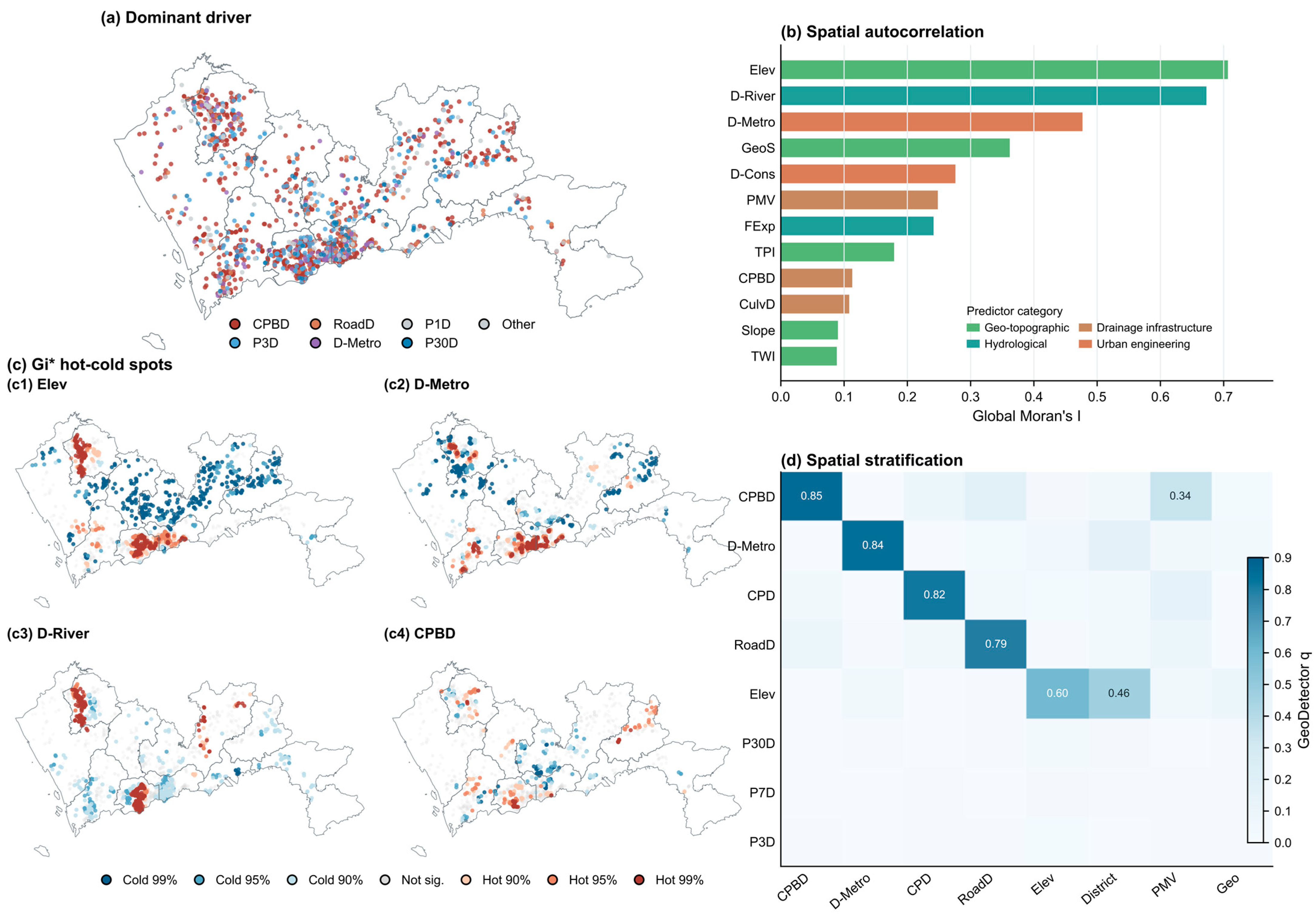
(2) Spatial SHAP analysis was used to characterize the geographic organization of model explanations. SHAP values were exported for the mapped grid and were separately summarized at observed collapse locations. For each collapse event, the dominant positive model attribution was defined as the predictor with the largest positive SHAP contribution:

$$d_i = \arg \underset{j:\hspace{0.17em}{\mathsf{\varphi }}_{\mathit{ij}}>0}{\max }{\mathsf{\varphi }}_{\mathit{ij}}$$

(6)

This definition allowed each collapse location to be interpreted in terms of the predictor that contributed most positively to its predicted susceptibility. For example, a site dominated by pipe burial depth indicates a different model-attribution pathway from a site dominated by antecedent rainfall, road density, terrain, or metro proximity. Samples without positive SHAP contributions were treated as having no positive dominant driver.

(3) Spatial autocorrelation in predictor-specific SHAP values was assessed using Global Moran’s I. For predictor $j$, Moran’s I was calculated as

$$M_j={\displaystyle \frac{n}{S_0}}{\displaystyle \frac{{\displaystyle {\sum }_{i=1}^n}{\displaystyle {\sum }_{k=1}^n}{w}_{\mathrm{ik}}\left({\mathsf{\varphi }}_{\mathit{ij}}-{\bar{\mathsf{\varphi }}}_j\right)\left({\mathsf{\varphi }}_{\mathrm{kj}}-{\overline{ \mathsf{\varphi }}}_j\right)}{{\displaystyle {\sum }_{i=1}^n}{\left({\mathsf{\varphi }}_{\mathit{ij}}-{\bar{\mathsf{\varphi }}}_j\right)}^2}}$$

(7)

where $M_j$ is the Moran’s I statistic for the SHAP values of predictor $j$, $w_{\mathrm{ik}}$ is the spatial weight between locations $i$ and $k$, $S_0=\sum _i\sum _k{w}_{\mathrm{ik}}$, and ${\bar{\mathsf{\varphi }}}_j$ is the mean SHAP value of predictor $j$. Local Moran’s I and Getis-Ord Gi* were then used to identify local clusters, spatial outliers, and hot or cold spots of SHAP contribution. GeoDetector was further applied to test whether SHAP-value heterogeneity was stratified by district, terrain, infrastructure, pipe, flood, metro, and construction-distance classes. The GeoDetector $q$-statistic was expressed as

$$q =1-{\displaystyle \frac{{\displaystyle {\sum }_{\mathrm{h}=1}^L}{N}_{\mathrm{h}}{\mathsf{\sigma }}_{\mathrm{h}}^2}{N{\mathsf{\sigma }}^2}}$$

(8)

where $L$ is the number of strata, $N_{\mathrm{h}}$ and ${\mathsf{\sigma }}_{\mathrm{h}}^2$ are the sample size and variance of SHAP values within stratum $\mathrm{h}$, and $N$ and ${\mathsf{\sigma }}^2$ are the corresponding values for the whole study area. A larger $q$ value indicates stronger stratified heterogeneity. These spatial statistics were interpreted as evidence of spatially organized model behaviors, not as direct causal proof.

2.7.2. Partial Dependence, ICE, and Interaction Analysis

Partial dependence plots (PDPs) and individual conditional expectation (ICE) curves were used to examine nonlinear and sample-specific responses of the selected model [80,81]. Unlike SHAP, which decomposes individual predictions into feature contributions, PDP and ICE analyses evaluate changes in predicted susceptibility as selected predictors are varied while the remaining predictors retain their observed values. These analyses were used to examine whether the model exhibited threshold-like responses and conditional patterns consistent with plausible hydro-infrastructure processes.

For a target predictor subset $S$, the partial dependence function was defined as

$${\widehat{f}}_S\left(\mathbf{z}\right)={\displaystyle \frac{1}{n}}{\displaystyle {\sum }_{i=1}^n}\widehat{f}\left(\mathbf{z},{\mathbf{x}}_{i,C}\right)$$

(9)

where $C$ is the complement of $S$, $\mathbf{z}$ is a fixed value or vector of values for the predictors in $S$, and ${\mathbf{x}}_{i,C}$ contains the observed values of the remaining predictors for sample $i$. The corresponding ICE function for sample $i$ was defined as

$${\widehat{f}}_S^{\left(i\right)}\left(\mathbf{z}\right)=\widehat{f}\left(\mathbf{z},{\mathbf{x}}_{i,C}\right)$$

(10)

The PDP therefore represents the model-averaged marginal response, whereas ICE curves retain sample-specific responses and reveal whether the average PDP masks heterogeneous local behaviors. In this study, PDP and ICE outputs were interpreted on the predicted-probability scale.

One-dimensional PDP-ICE analysis focused on key predictors selected from the explanatory workflow, including pipe burial depth, road density, 30-day rainfall, metro distance, elevation, and pipe density. Predictor grids were constructed from the 2nd to 98th percentiles of the hold-out distribution to reduce the influence of extreme outliers. ICE curves were calculated on a random subset of hold-out samples, and the PDP was obtained by averaging the ICE curves at each grid value.

Two-dimensional PDP surfaces were generated to evaluate examine joint model-response patterns for mechanism-relevant predictor pairs related to predicted UGC susceptibility. For a predictor pair $\left(a,b\right)$, the two-dimensional response surface was calculated as

$${\widehat{f}}_{a,b}\left(z_a,z_b\right)={\displaystyle \frac{1}{n}}{\displaystyle {\sum }_{i=1}^n}\widehat{f}\left(z_a,z_b,{\mathbf{x}}_{i,-\{a,b\}}\right)$$

(11)

where $z_a$ and $z_b$ are fixed grid values for predictors $a$ and $b$, and ${\mathbf{x}}_{i,-\{a,b\}}$ denotes the observed values of all remaining predictors for sample $i$. The two-dimensional PDP analysis focused on three mechanism-oriented pairs. Grid values were taken from the 3rd to 97th percentiles of the hold-out distributions.

These two-dimensional response surfaces were interpreted as model-based diagnostics of coupled hydro-infrastructure response patterns rather than as direct causal experiments. The P30D × CPBD surface was used to examine whether the model assigned higher susceptibility when elevated antecedent rainfall coincided with deeply buried drainage pipelines. The CPBD × RoadD surface assessed whether burial-depth-related model responses became stronger as road density increased. The CPBD × D-Metro surface assessed whether model responses associated with pipe burial depth varied with proximity to metro corridors.

Because PDPs may evaluate uncommon predictor combinations when predictors are correlated, accumulated local effects (ALE) curves were calculated as a feature-dependence sensitivity analysis. ALE was evaluated for CPBD, CPD, RoadD, P30D, D-Metro, and Elev using adaptive quantile-based binning. The numbers of bins were 13 for CPBD and CPD, 8 for RoadD, and 20 for P30D, D-Metro, and Elev. Uncertainty was assessed using 200 bootstrap resamples. Mean-centred PDP curves were compared with the corresponding ALE curves to evaluate the robustness of response direction while avoiding interpretation of exact effect magnitudes or breakpoint locations. The ALE comparisons and observed-support diagnostics are provided in Supplementary Figures S9 and S10 and Supplementary Table S9.

3. Results

3.1. Model Evaluation: Predictive Performance, Validation, Calibration, and Robustness

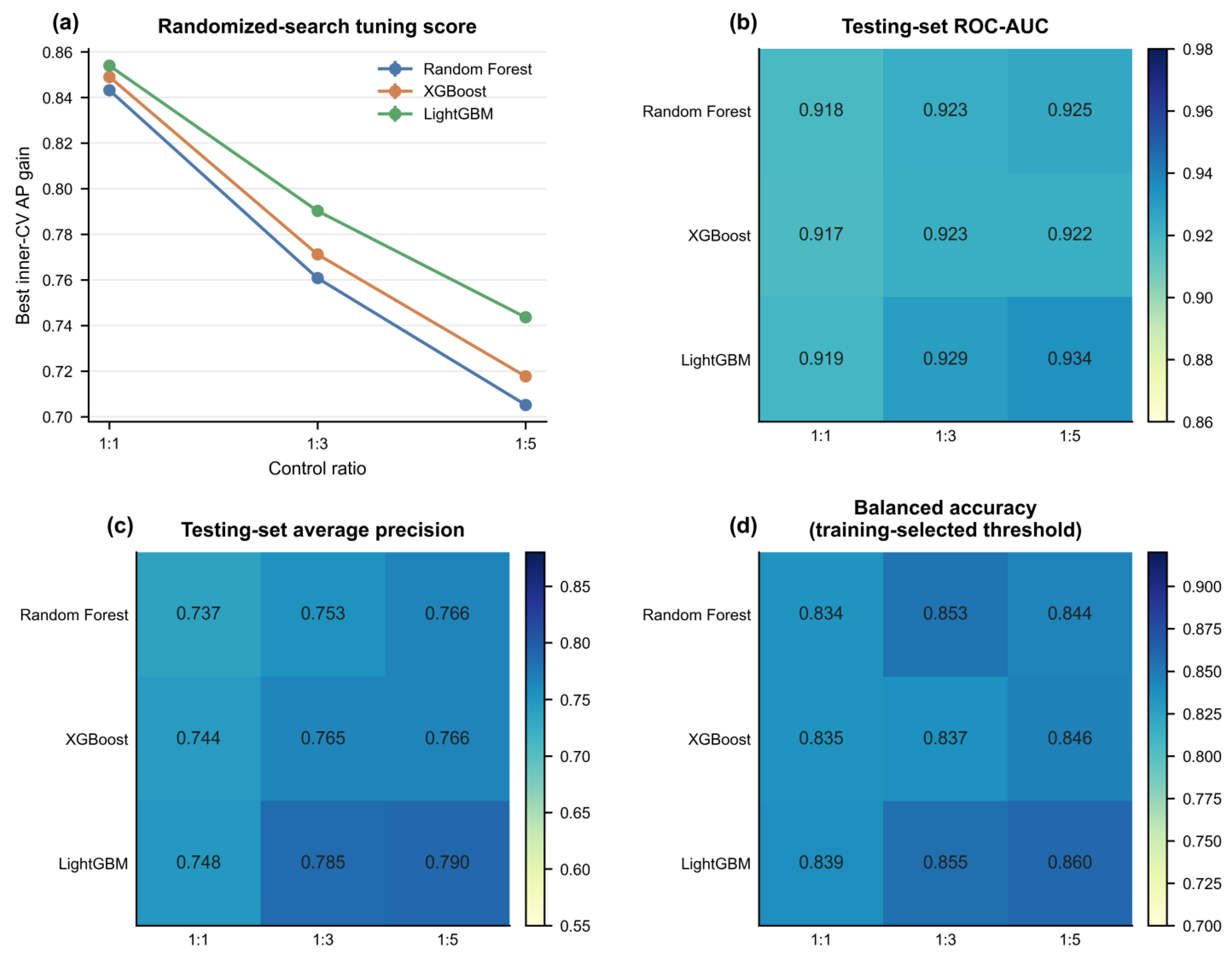
Across the nine algorithm–sampling-ratio configurations, LightGBM with a 1:5 collapse-to-background-control ratio achieved the best overall performance on the reserved random hold-out set (Figure 4; Supplementary Table S4). The selected configuration achieved ROC-AUC = 0.934 and AP = 0.790. At thresholds selected exclusively from out-of-fold predictions within the training partition, the model achieved BA = 0.860 at the BA-optimised threshold of 0.119 and F1 = 0.699 at the F1-optimised threshold of 0.272. The difference between the two thresholds reflects the different operating objectives of BA and F1 under the imbalanced presence–background design; neither threshold represents a universal physical-risk boundary. The principal validation and calibration results are summarised in

Table 2. Summary of model performance and calibration under different validation designs.

Validation Design	ROC-AUC	AP	BA	F1	Brier Score	Calibration Slope
Random 75/25 tests	0.934	0.790	0.860	0.699	0.068	0.948
District LODO	0.905 ± 0.023	0.676 ± 0.177	0.817 ± 0.031	0.610 ± 0.159	0.079	0.841
Temporal tests	0.884	0.649	0.813	0.633	0.092	0.722

.

Performance decreased under spatially and temporally separated evaluation, confirming that the random hold-out result was a comparatively optimistic interpolation benchmark. LODO validation yielded mean ROC-AUC = 0.905 ± 0.023 and BA = 0.817 ± 0.031, whereas the larger between-district variation in AP and F1 indicated greater heterogeneity in precision–recall performance across districts. Under forward temporal hold-out validation, ROC-AUC, AP, BA, and F1 were 0.884, 0.649, 0.813, and 0.633, respectively. Year-specific ROC-AUC declined from 0.916 in 2022 to 0.833 in 2024, indicating increasing temporal transfer difficulty while retaining useful discrimination in the later test period. District-specific and year-specific results are reported in Supplementary Figure S5 and Table S5.

Probability calibration showed a similar transfer pattern. On the random hold-out set, the model achieved a Brier score of 0.068, a Brier skill score of 0.507, an ECE of 0.015, and a calibration slope of 0.948, indicating relatively close agreement between predicted susceptibility scores and observed frequencies within the sampled evaluation distribution. Under LODO and temporal validation, Brier scores increased to 0.079 and 0.092, Brier skill scores decreased to 0.429 and 0.340, and calibration slopes declined to 0.841 and 0.722, respectively. ECE remained low under LODO validation at 0.017 but increased to 0.037 under temporal transfer. Thus, the model retained positive calibration skill relative to a prevalence-only reference under all three designs, although probability reliability weakened under spatial and especially temporal domain shifts. Because the analysis used a presence–background sampling design, these outputs represent susceptibility scores conditional on the sampled evaluation prevalence rather than absolute annual collapse probabilities. Reliability curves and the complete calibration statistics are shown in Supplementary Figure S6 and Table S6.

The background-control sensitivity analyses further indicated that the principal findings were not determined by a single exclusion distance or pseudo-date realisation. Across exclusion buffers of 50–200 m, ROC-AUC ranged from 0.926 to 0.938 and AP from 0.771 to 0.813. CPBD, RoadD, and P30D retained the first three SHAP ranks under every buffer setting, while the complete SHAP ranking remained highly consistent with the 150 m reference configuration, with Kendall’s tau ranging from 0.926 to 0.958 and Spearman correlations of mean absolute SHAP values ranging from 0.982 to 0.991. Across 20 repeated pseudo-event-date assignments, ROC-AUC was 0.929 ± 0.003 and AP was 0.779 ± 0.010. SHAP explanations were also stable, with the mean Kendall rank similarity of 0.915 ± 0.028 and mean Spearman correlation of 0.980 ± 0.011 relative to the baseline assignment. CPBD ranked first in all repetitions, while RoadD and P30D remained among the four leading predictors. Full buffer-distance and pseudo-date sensitivity results are reported in Supplementary Figures S7 and S8 and Tables S7 and S8.

The selected model combined strong random-hold-out discrimination with lower but retained spatial and temporal transfer performance, positive calibration skill under all validation designs, and stable core predictor rankings across background-control sensitivity analyses. The decline in temporal discrimination and calibration nevertheless indicates that transfer results should be interpreted more conservatively than the random hold-out benchmark.

3.2. Rainfall-Scenario Susceptibility Mapping

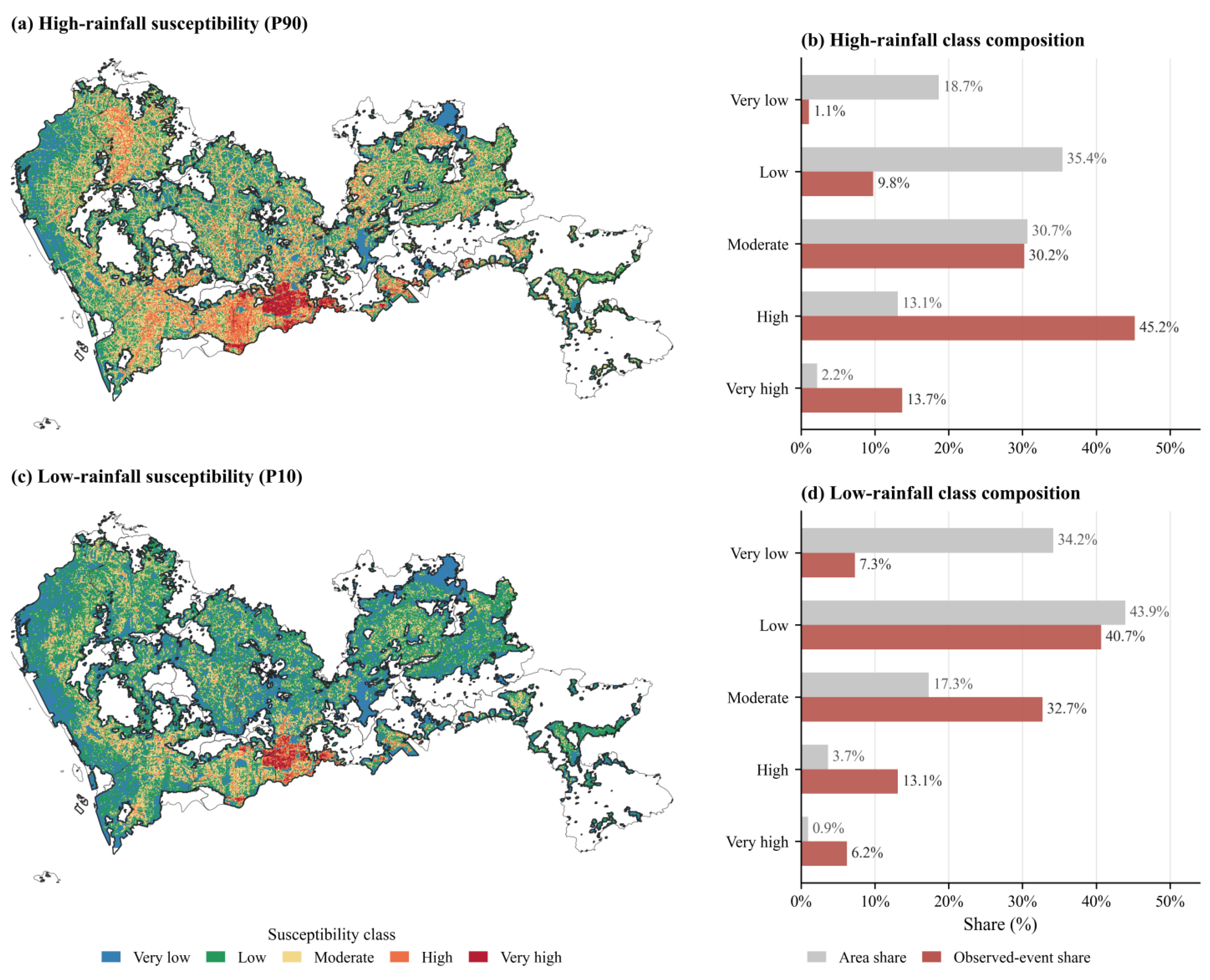
As UGC susceptibility was expected to vary with rainfall forcing, 1-day, 3-day, 7-day, and 30-day antecedent rainfall were incorporated as dynamic predictors. To evaluate how predicted susceptibility changes under different rainfall settings, scenario-based mapping was performed using the 10th-percentile low-rainfall and 90th-percentile high-rainfall settings derived from the observed collapse-event rainfall distribution (Figure 5).

The selected LightGBM 1:5 model was applied to the complete built-up grid domain. To ensure direct comparison between rainfall scenarios, the P10 and P90 probability maps were classified into five susceptibility levels using a common set of Jenks natural-break thresholds [82]. The common class thresholds and class-specific area and event shares are listed in Supplementary Table S10. Under the low-rainfall scenario, the High and Very high classes occupied only 4.60% of the mapped area but contained 19.32% of observed events. This result indicates that a small subset of the urban fabric retains elevated baseline susceptibility associated with static geomorphic and structural conditions, including utility corridors, road density, pipe burial conditions, and drainage constraints.

Under the P90 setting, the combined High and Very high classes expanded to 15.26% of the mapped area, while the proportion of recorded collapse locations within these classes increased from 19.32% to 58.92%. This redistribution indicates that high antecedent rainfall substantially increased modelled susceptibility in parts of the built-up domain. This pattern is consistent with rainfall acting as a potential trigger superimposed on spatially variable subsurface vulnerability, where prolonged wetting and storm input may increase pore-water pressure, seepage gradients, and the instability of pre-existing weak zones.

3.3. Global SHAP Importance and Grouped Model Contributions

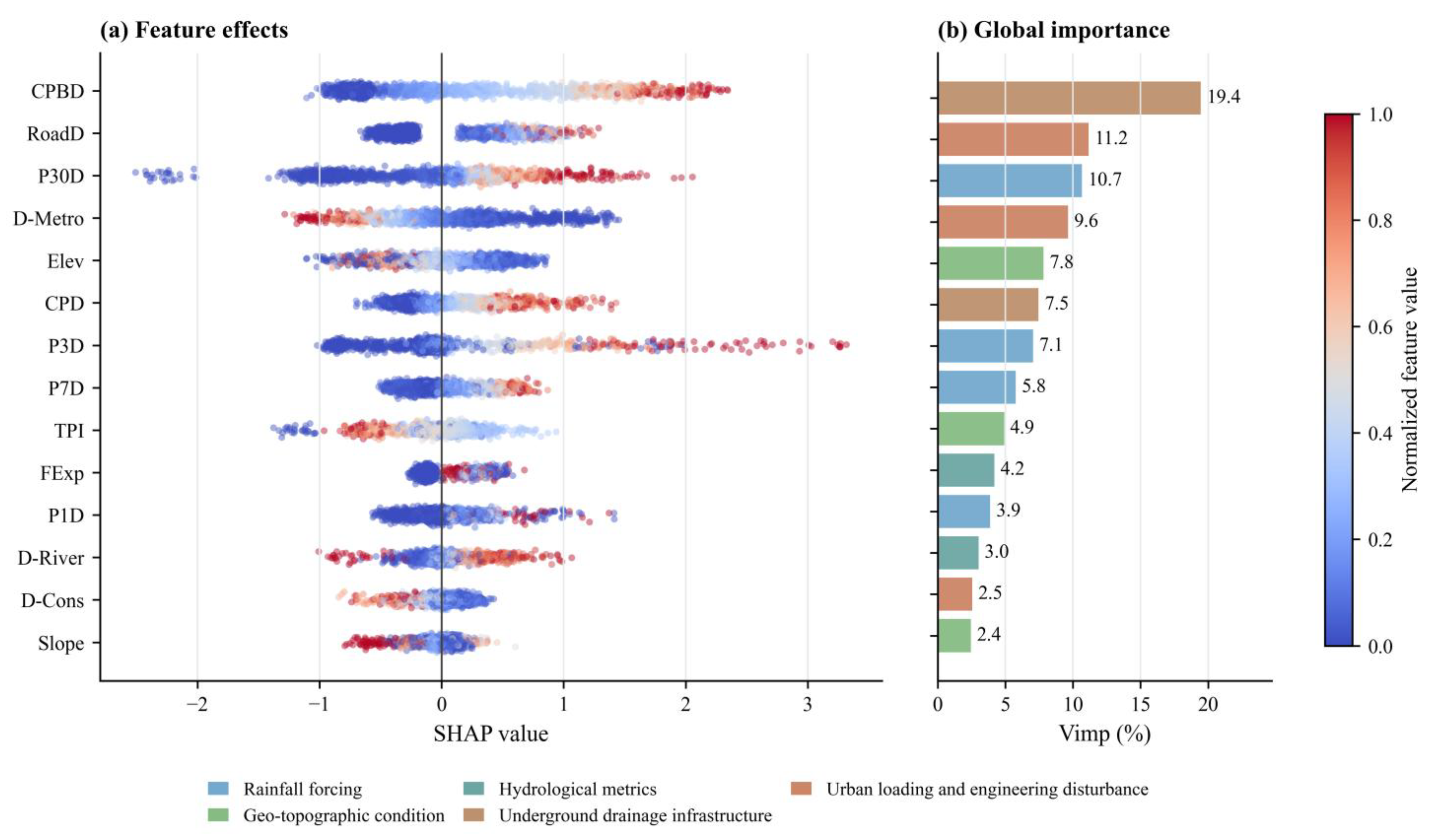
The global SHAP results shown in Figure 6 identified a small set of dominant predictors in the selected model. The largest global contribution was associated with pipe burial depth, with a mean absolute SHAP value of 0.736. This result indicates that the vertical position of core pipelines relative to the ground surface and surrounding soils was strongly associated with predicted collapse susceptibility. Physically, pipe burial depth is linked to trench excavation, backfill quality, overburden stress, leakage pathways, local hydraulic head, and the depth at which soil erosion or cavity growth may initiate. A buried pipeline is therefore an engineered discontinuity that can alter seepage paths and soil structure.

Road density ranked second, with a mean absolute SHAP value of 0.423. Dense road networks tend to coincide with buried utilities, drainage conduits, pavement cuts, repeated excavation, and heavy traffic loading. These conditions can increase the number of pipe–soil interfaces and weak backfilled zones, while also reducing the visibility of slow subsurface erosion before surface failure occurs. The road-density response may reflect the structural complexity of dense urban corridors.

Rainfall variables formed the other major component of model explanation. The 30-day rainfall variable ranked third, with a mean absolute SHAP value of 0.404, while 3-day, 7-day, and 1-day rainfall also contributed to the model. The high rank of 30-day rainfall suggests that antecedent wetness is a key preparatory condition. Long-duration rainfall can reduce matric suction, raise local groundwater levels, soften fill materials, and increase the probability of seepage-induced internal erosion. Shorter rainfall windows may represent event-scale rainfall inputs associated with short-term susceptibility changes that can surcharge drainage systems and accelerate the migration of fine particles through pre-existing voids, joints, or pipe defects.

Metro distance, elevation, and pipe density were also among the leading predictors, with mean absolute SHAP values of 0.365, 0.296, and 0.282, respectively. Metro distance captures the influence of major underground engineering corridors, including excavation disturbance, local dewatering history, ground improvement, and changes in the stress and drainage environment. Elevation represents broader topographic control over runoff accumulation, hydraulic gradients, and drainage efficiency. Pipe density measures the concentration of potential leakage interfaces and trench-backfill zones. Together, these variables indicate that collapse susceptibility is shaped by the coupling of hydrological forcing and engineered subsurface disturbance.

Grouped SHAP analysis showed that underground drainage infrastructure made the largest contribution (26.01%), followed by rainfall forcing (25.13%), urban loading and engineering disturbance (21.44%), geo-topographic conditions (16.14%), and hydrological and flood-related conditions (11.28%). The near-equal contributions of the pipeline and rainfall groups are important because they indicate that susceptibility cannot be explained by rainfall alone or by infrastructure alone. Instead, the model captured the pattern consistent with hydro-infrastructure coupling in which pipe-trench systems and urban drainage pathways provide the physical setting for collapse, while rainfall is strongly associated with the timing and intensity of hydrological activation.

3.4. Nonlinear Response Surfaces and Feature-Dependence Sensitivity

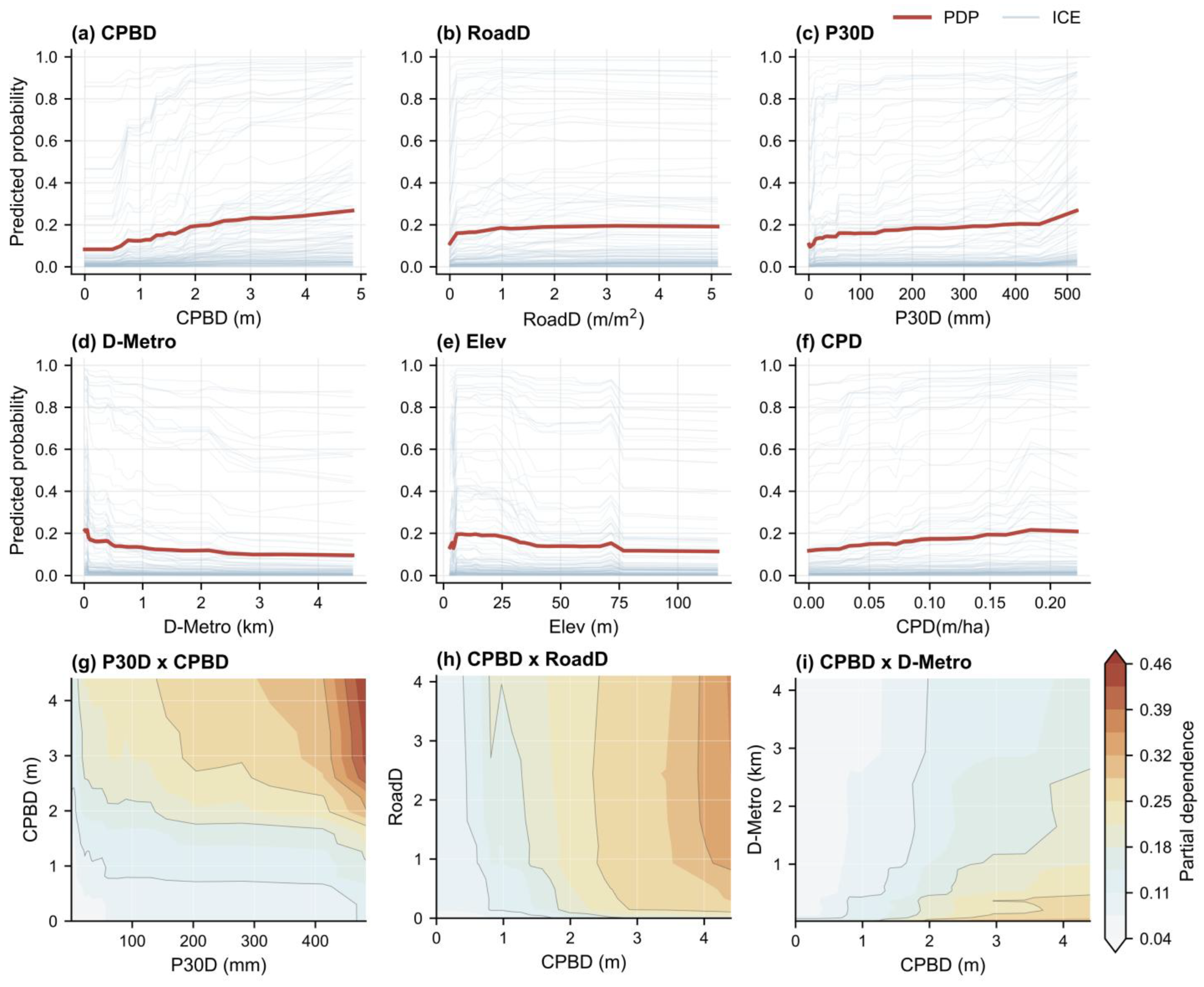
The PDP–ICE and two-dimensional response diagnostics shown in Figure 7 were used to examine how the selected LightGBM model transformed key predictors into predicted collapse probability. In the one-dimensional panels, the red partial dependence plot (PDP) represents the model-averaged marginal response, whereas the pale individual conditional expectation (ICE) curves represent sample-specific responses under the same predictor perturbation. Pipe burial depth, road density, pipe density, and 30-day rainfall generally increased predicted susceptibility over much of their evaluated ranges, while metro distance showed an inverse distance effect and elevation acted mainly as a contextual modifier. The wide spread of ICE curves indicates substantial local heterogeneity, meaning that the same predictor change can produce different risk responses depending on the surrounding combination of terrain, rainfall state, drainage infrastructure, road density, and engineering disturbance.

Pipe burial depth showed the strongest increase among the one-dimensional responses. This pattern does not imply that deeper pipes are intrinsically hazardous in isolation. Rather, deeper drainage corridors may be associated with larger disturbed trench-backfill volumes, more complex pipe–soil interfaces, and less visible subsurface deformation before surface expression. When leakage or seepage occurs, greater overburden may delay the surface manifestation of internal erosion or void development. Such cases are therefore more likely to be represented in municipal collapse inventories when deformation finally reaches the road surface.

Road density also increased predicted probability, reflecting the role of road corridors as integrated disturbance zones where utilities, pavement reinstatement, drainage structures, traffic loading, and water-ingress pathways are concentrated. Pipe density showed a gradual upward response, but its widely dispersed ICE curves indicate that dense pipeline networks showed a stronger joint contribution to UGC when combined with burial depth, rainfall, terrain, or road-corridor conditions.

The 30-day rainfall response increased toward the upper antecedent-rainfall range, consistent with its interpretation as a preparatory hydrological condition. Prolonged rainfall can increase soil moisture, reduce matric suction, soften disturbed fill, raise shallow groundwater levels, and sustain seepage through pipe defects or trench backfill. D-Metro decreased with distance from metro corridors, suggesting elevated susceptibility near underground engineering zones. Rather than implying that metro lines independently trigger failure, the distance-to-metro variable serves as a proxy for underground engineering footprints, capturing the cumulative impacts of subsurface excavation, dewatering, and geotechnical stress perturbations. Meanwhile, the narrow, non-monotonic response of elevation confirms that topographic context operates as a spatial modifier, adjusting collapse susceptibility via its joint interaction with local drainage pathways and construction intensity.

The two-dimensional PDP surfaces showed that the highest predicted susceptibility occurred under specific combinations of predictor values. The 30-day rainfall and pipe burial depth surface had the widest response range, from 0.036 to 0.457, and reached its maximum where 30-day rainfall was approximately 482.7 mm and pipe burial depth was approximately 4.40 m. This surface is consistent with a coupled hydro-infrastructure pathway in which high antecedent rainfall increases wetness and hydraulic gradients, while deep core pipelines represent engineered discontinuities with deeper trench backfill and delayed surface expression of void development. The pipe burial-depth and road-density interaction surface ranged from 0.050 to 0.357 and indicates that buried-pipeline depth becomes more consequential in dense road corridors. The interaction surface between pipe burial depth and metro distance ranged from 0.039 to 0.314 and suggests that deep drainage pipelines and metro-adjacent engineering environments jointly increase predicted susceptibility. Overall, the PDP-ICE diagnostics indicate that the fitted model represents susceptibility through nonlinear and context-dependent response patterns rather than by independent single-factor effects.

As a feature-dependence sensitivity analysis, ALE curves showed broad directional agreement with the corresponding centred PDPs for CPBD, CPD, RoadD, P30D, D-Metro, and Elev. Differences were mainly observed in effect magnitude, with the largest divergence occurring in the upper tail of P30D. The observed-support rates for the P30D × CPBD, CPBD × RoadD, and CPBD × D-Metro surfaces were 85.2%, 77.4%, and 81.9%, respectively, indicating that most evaluated surface cells were supported by at least five observed test samples. These diagnostics support interpretation of the broad response directions but not precise effect magnitudes or breakpoint locations. Detailed ALE–PDP comparisons are shown in Supplementary Figure S9, and observed-support overlays for the two-dimensional response surfaces are shown in Supplementary Figure S10. The corresponding binning and support statistics are listed in Supplementary Table S9.

3.5. Spatial SHAP Heterogeneity and District-Level Patterns

Spatial SHAP analysis at observed collapse locations (Figure 8a) showed that the global UGC contributors were expressed unevenly across the city. Pipe burial depth had the largest mean absolute SHAP contribution at collapse sites, with a value of 1.106, and its mean SHAP value was positive at 0.993. Positive SHAP contributions occurred at 83.52% of collapse locations. Thus, CPBD shifted the model output above its baseline at most recorded collapse locations. Road density showed a mean absolute SHAP value of 0.649 and a positive-share value of 79.08%, indicating that road-corridor conditions frequently amplified local modelled susceptibility.

Rainfall-related SHAP contributions were also predominantly positive at recorded collapse locations. The 30-day rainfall variable had a positive-share value of 84.71%, whereas the 3-day rainfall variable had a positive-share value of 63.43%. This contrast suggests that antecedent rainfall was more consistently associated with local susceptibility increases than the shorter trigger window, although both were important. The finding is consistent with a mechanism in which cumulative wetting establishes weak hydraulic and geotechnical conditions, while short-term rainfall contributes to susceptibility increases in selected locations.

The strength of global spatial autocorrelation differed substantially among predictor-specific SHAP values. The strongest global spatial autocorrelation was observed for Elev (I = 0.707), followed by D-River (I = 0.673) and D-Metro (I = 0.477). GeoS, D-Cons, PMV, FExp, and TPI also showed significant positive spatial autocorrelation. These results indicate that terrain, hydrological proximity, and major underground engineering conditions form broad spatial structures in the SHAP explanation surface.

In contrast, pipe burial depth and road density had lower but still significant Moran’s I values of 0.113 and 0.084, respectively. This difference is meaningful: pipeline burial conditions and road-corridor effects are highly local and may change across short distances because of pipe age, trench history, material type, road hierarchy, and maintenance records. The Gi* maps showed overlapping hot spots of positive D-Metro and CPBD SHAP values in the highly urbanized areas of Futian and Luohu (Figure 8(c2,c4)). These high SHAP values indicate that within these mature downtown corridors, deeply buried pipelines and adjacent underground transit engineering do not act as isolated structural attributes; rather, they act as locally important contributors to predicted susceptibility above the citywide baseline.

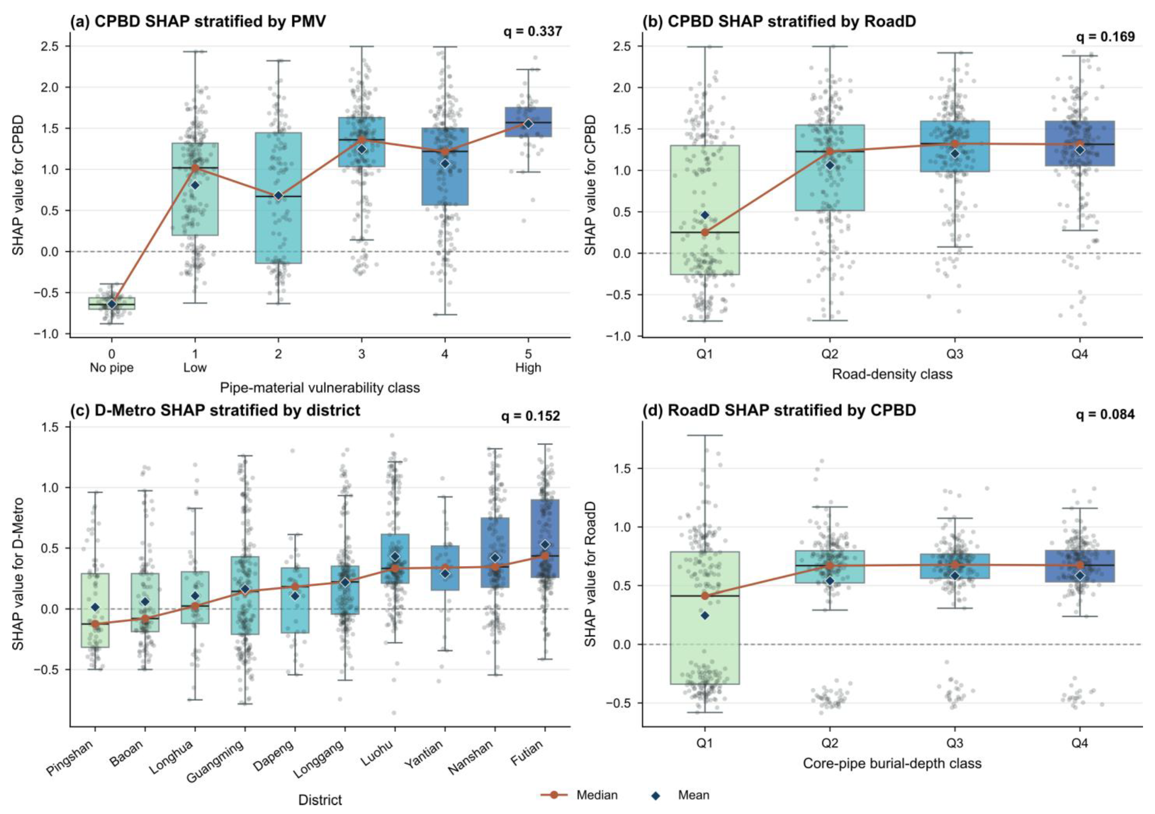
GeoDetector analysis further showed stratified heterogeneity in predictor-specific SHAP values (Figure 8d). In the cross-stratifier analysis, CPBD SHAP values showed the strongest stratification by PMV class (q = 0.337), followed by RoadD class (q = 0.169) (Figure 9a,b). D-Metro SHAP was stratified by district (q = 0.152), suggesting that metro-related effects were conditioned by broader urban morphology, construction history and underground development intensity rather than by administrative boundaries themselves. RoadD SHAP values showed weaker stratification across CPBD classes (q = 0.084; Figure 9d). Overall, the cross-stratifier GeoDetector results indicate that SHAP responses were not only predictor-specific but also context-dependent, supporting the interpretation of UGC susceptibility as a coupled hydro-infrastructure process rather than a set of isolated factor effects.

4. Discussion

4.1. Predictive Reliability, Generalization, and Calibration

Predictive discrimination, probability calibration, and geotechnical interpretation address different questions and should not be treated as interchangeable evidence. The random 75/25 hold-out produced the highest discrimination, with an ROC-AUC of 0.934. Performance decreased under leave-one-district-out spatial validation and forward temporal holdout testing, with ROC-AUC values of 0.905 ± 0.023 and 0.884, respectively (Table 2; Supplementary Figure S5 and Table S5). This decline suggests that the random split may have benefited partly from interpolation among samples that shared similar urban, infrastructural, rainfall, and reporting contexts. Nevertheless, the retained discrimination under district-based and temporal separation suggests that the selected predictor system contains information that is transferable within the Shenzhen modelling domain.

Probability calibration showed a similar pattern. The calibration slope decreased from 0.948 under random testing to 0.841 under district-based validation and 0.722 under temporal holdout testing, while all three Brier skill scores remained positive relative to the prevalence-only reference model (Table 2; Supplementary Figure S6 and Table S6). Thus, the model provided useful relative susceptibility scores, but probability reliability weakened under spatial and temporal domain shifts. Because the model was developed under a presence–background sampling design, its outputs should be interpreted primarily as relative susceptibility scores within the sampled evaluation distribution rather than as absolute annual collapse probabilities for Shenzhen.

The buffer-distance and pseudo-event-date sensitivity analyses further showed that the principal performance metrics and leading SHAP rankings were not determined by a single background-construction setting (Supplementary Figures S7 and S8; Supplementary Tables S7 and S8). However, this robustness should not be interpreted as proof that the background labels are error-free or that the inferred predictor relationships are physically causal. The validation, calibration, and sensitivity analyses increase confidence in the predictive robustness of the model. Geotechnical interpretation, however, requires a separate line of reasoning based on consistency with established physical processes and independent field evidence.

4.2. Dynamic Rainfall Impacts on UGC Susceptibility

The rainfall-scenario results support the interpretation of UGC susceptibility as a rainfall-conditioned rather than purely static modelled state. Scenario mapping indicates that the model predicted an upward shift in susceptibility under the P90 rainfall setting. The selected LightGBM model represented a baseline city-scale susceptibility pattern and assigned the largest P90-related increases to areas characterized by sensitive infrastructure and terrain conditions. High and very high susceptibility zones expanded from 4.60% of the mapped built-up area under the low-rainfall scenario to 15.26% under the high-rainfall scenario, and the proportion of historical collapse locations falling within these zones increased from 19.32% to 58.92% (Figure 5; Supplementary Table S10). This shift indicates that rainfall did not act as a uniform hazard layer in the scenario analysis. Instead, high antecedent rainfall appeared to amplify predicted susceptibility in areas where underground drainage infrastructure, road-corridor disturbance, terrain-controlled water accumulation, and engineering disturbance were already associated with elevated baseline susceptibility.

This interpretation is consistent with empirical and experimental evidence that heavy rainfall can amplify failure in urban underground infrastructure systems. A review of 378 heavy-rainfall-related failures of urban underground infrastructure in China showed that such failures were strongly conditioned by geological, engineering, and urban-construction settings [8]. This rainfall-conditioned response was also reflected in the high global importance of P30D and its generally increasing upper-range response in the PDP and ALE diagnostics (Figure 6 and Figure 7c; Supplementary Figure S9c and Table S9). Moreover, the model’s stronger response to high antecedent-rainfall values is consistent with failure processes observed in scaled physical experiments and numerical simulations. For example, physical model tests have shown that rainfall intensity affects the development of erosion zones and sinkholes above damaged sewer pipes [11]. Repetitive heavy rainfall has also been reported to promote urban road collapse when damaged sewer pipes provide pathways for soil loss [12]. These comparisons suggest that the association between rainfall and predicted UGC susceptibility is conditioned by disturbed engineered subsurface settings.

This model-inferred pattern is consistent with established hydro-geotechnical processes. Prolonged rainfall may reduce matric suction in initially unsaturated backfill. Where positive pore-water pressures develop, it may also reduce effective stress in accordance with Terzaghi’s principle. Increased hydraulic gradients and seepage forces around pipe defects or disturbed backfill may subsequently promote fine-particle migration, internal erosion, progressive cavity enlargement, and delayed surface deformation under favorable soil and hydraulic conditions. A finite-element study incorporating Terzaghi’s principle illustrated how pore-pressure changes and effective-stress redistribution can produce non-uniform underground deformation under non-oedometric conditions [83]. It is cited here only as a mechanical analogy, because tunnel-induced deformation and UGC are distinct engineering problems.

Consequently, the rainfall-conditioned model responses highlight the value of dynamic susceptibility mapping for time-varying UGC screening, extending conventional static susceptibility zoning towards rainfall-informed assessment. In rainfall-induced landslide studies, susceptibility maps have been combined with rainfall thresholds or real-time rainfall windows to distinguish spatial predisposition from temporal triggering [23,24,25]. The framework therefore transfers the conceptual distinction between spatial predisposition and temporal forcing from dynamic landslide research to an infrastructure-mediated urban subsurface setting, rather than assuming that UGC follows a slope-failure mechanism. Static geo-topographic and infrastructure predictors represent baseline spatial predisposition, whereas event-specific rainfall windows represent temporal forcing associated with upward shifts in modelled susceptibility. By assigning antecedent rainfall to both collapse samples and year-constrained background controls, the present framework extends this dynamic logic to the infrastructure-mediated urban geohazard.

4.3. Pipe Burial Depth and Road Corridors as Proxies for Engineered Subsurface Discontinuity

Pipe burial depth was the highest-ranked model predictor in the selected city-level model. This finding should not be interpreted as evidence that depth alone mechanically causes collapse. A more defensible interpretation is that pipe burial depth acts as a proxy for the vertical structure and construction history of engineered discontinuities in the urban subsurface. Deeper drainage corridors usually require deeper trench excavation, larger volumes of backfill, longer pipe–soil interfaces, and more complex interactions among overburden stress, groundwater, and leakage pathways. If leakage, surcharge, or defect-induced inflow occurs, soil particles may be mobilized at depth before deformation becomes visible at the surface.

In paved road environments, subsurface erosion and progressive cavity development may remain undetected until deformation reaches the surface, a process supported by physical and numerical studies of pipe-induced cavity development [19,20]. The location of subsurface structures affects the development of underground cavities induced by internal erosion from sewer-pipe breakage [20]. Physical model tests of damaged sewer pipes have reproduced underground cavities and ground cave-ins, with the resulting ground response varying according to soil type and density [19]. More recent experimental and numerical studies have linked pipeline defects, leakage, burial depth, groundwater level, defect-opening size, and internal pipe pressure to seepage erosion and ground collapse [14,15]. Furthermore, pipeline-leakage-induced road collapse has been described as a staged process involving particle detachment, seepage-channel formation, void development, and eventual surface collapse [10]. The city-scale dominance of pipe burial depth, together with its stable first-place SHAP ranking across the buffer-distance and pseudo-date sensitivity analyses, therefore provides model evidence consistent with mechanisms repeatedly observed at physical-model and site-process scales (Figure 6; Supplementary Figures S7 and S8; Supplementary Tables S7 and S8).

Road density was the second highest-ranked predictor and should be read as an urban-corridor index rather than a simple measure of road presence. Dense road networks are commonly associated with concentrations of buried utilities, drainage inlets, pavement cuts, trench reinstatement, maintenance excavations, traffic loading, and runoff routing along curbs and drains. This corridor-scale interpretation is consistent with nationwide analyses of urban road collapse in China, which identify pipeline defects, underground construction, and road-related disturbances as recurring contributors to collapse incidents [7]. It is also consistent with a machine-learning study in Shanghai where machine-learning susceptibility assessment was validated using geophysical detection, and underground pipeline structural problems were identified as highly influential [6]. Compared with these studies, the present analysis more explicitly separates road-corridor density, pipeline density, pipe burial depth, and pipe-material vulnerability, allowing the road signal to be interpreted as a corridor context that modifies pipeline-related collapse potential rather than as a stand-alone causal factor (Figure 7b,h; Supplementary Figures S9b and S10b; Supplementary Table S9).

4.4. Conditional Hydro-Infrastructure Patterns Indicated by PDP and Spatial SHAP Diagnostics

The PDP-ICE and two-dimensional PDP results show why global feature ranking is insufficient for interpretation. The interaction surface between 30-day rainfall (P30D) and pipe burial depth produced the widest model-response range, indicating that antecedent rainfall and deeply buried drainage corridors were associated with the strongest modelled susceptibility response (Figure 7g; Supplementary Figure S10a and Table S9). This pattern is consistent with a coupled hydro-infrastructure response in which prolonged rainfall increases wetness, reduces matric suction, and strengthens hydraulic gradients, while deeply buried pipeline corridors provide disturbed trench backfill and pipe–soil interfaces where internal erosion may initiate.

The CPBD × RoadD surface showed that burial-depth-related model responses became stronger in dense road corridors. This finding connects two mechanism-relevant predictor groups that are often discussed separately: leakage or seepage through pipe-trench systems and mechanical disturbance associated with road infrastructure. In a dense corridor, pavement reinstatement, repeated excavation, utility crowding, traffic loading, and drainage concentration may all reduce the buffering capacity of the subsurface. When such corridor conditions overlap with deeply buried drainage infrastructure, predicted susceptibility may increase in a pattern consistent with hidden cavity development and delayed surface expression. The interaction surface between pipe burial depth and metro distance adds a third mechanism-relevant pattern: pipeline-related vulnerability is stronger near major underground engineering corridors, where excavation history, ground improvement, stress redistribution, and altered drainage routes may have modified the subsurface state.

These interaction results improve the interpretability of the model as they connect predictive patterns to plausible process chains. SHAP provides local additive contributions and spatially organized explanation fields, whereas PDP and ICE curves diagnose the direction, nonlinearity, and heterogeneity of the model response [40,41]. In geohazard research, XAI methods have increasingly been used to reduce the gap between high predictive performance and physically interpretable susceptibility modelling [31]. This study extends this approach to an urban infrastructure-mediated collapse problem: spatial SHAP identifies where particular predictor contributions are locally dominant, while PDP-based surfaces diagnose whether the model response is consistent with coupled rainfall-pipeline-road-engineering pathways. This does not prove causality, but it provides a structured basis for formulating mechanism hypotheses that can be tested by CCTV pipe inspection, geophysical survey, borehole verification, or post-collapse forensic investigation.

A key caveat is that PDP perturbations are marginal and may evaluate predictor combinations that are uncommon in the observed city, particularly when CPBD, RoadD, CPD, and D-Metro co-vary along transport and utility corridors. The two-dimensional surfaces should therefore be interpreted as model-response diagnostics rather than as causal experiments. The broad directional agreement between ALE and centred PDP supports the qualitative response patterns, whereas differences in magnitude and upper-tail behaviour indicate that exact effect sizes and breakpoint locations remain uncertain (Supplementary Figure S9 and Table S9).

4.5. Spatial Heterogeneity and District-Specific Drivers

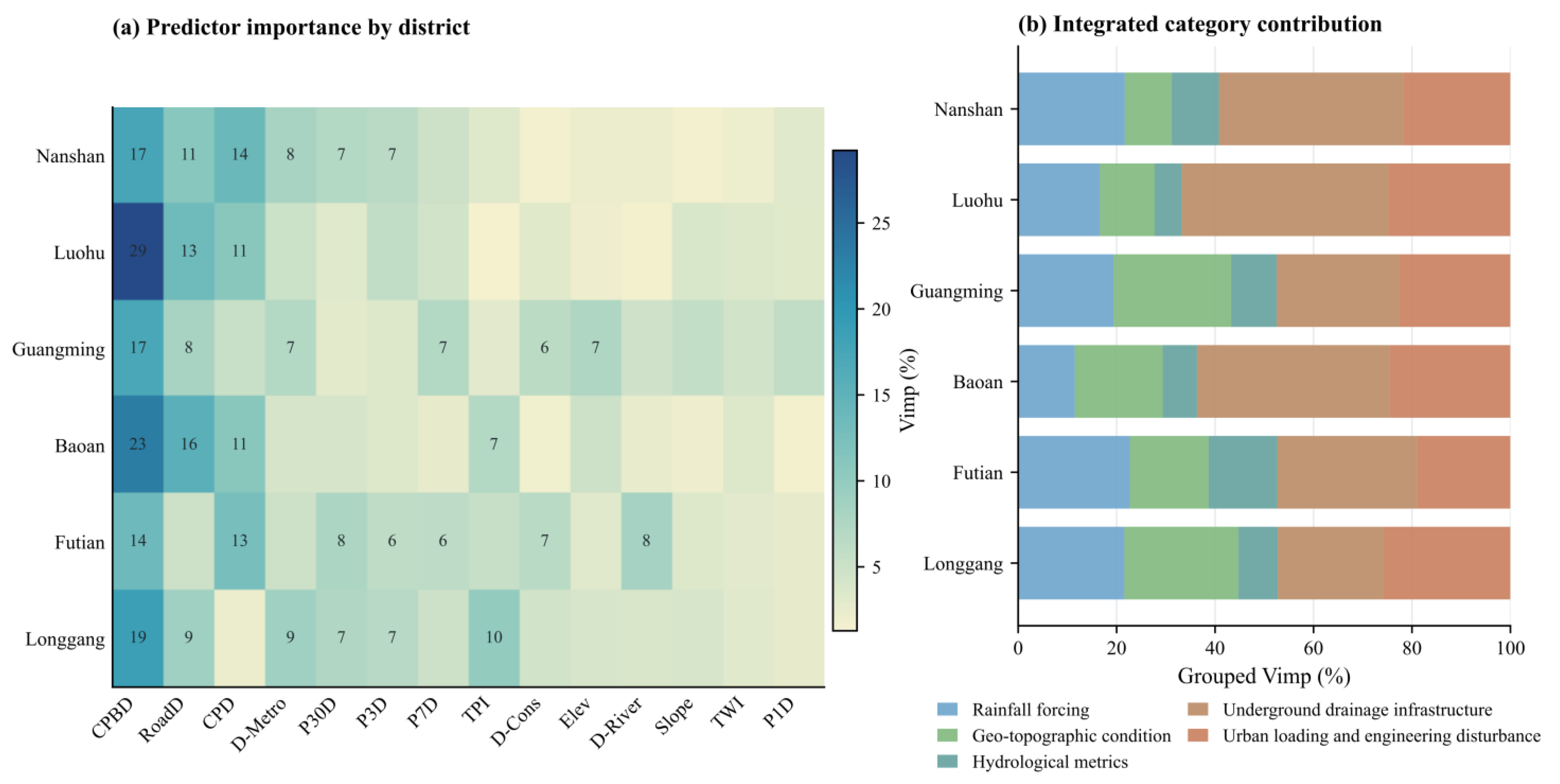
Spatial SHAP diagnostics showed that predictor-specific explanation patterns were unevenly organised across Shenzhen (Figure 8). District-level modelling further showed that the relative importance of the five mechanism groups varied among districts (Figure 10; Supplementary Figure S11 and Table S11). Broadly autocorrelated predictors, such as elevation, river distance, and metro distance, formed large-scale explanation structures, whereas pipe burial depth and road density showed lower but significant autocorrelation. This distinction is meaningful. Terrain and hydrological proximity vary gradually across the city, but pipeline burial conditions and road-corridor disturbances can change abruptly across short distances because of pipe age, trench history, maintenance records, material type, road hierarchy, and construction sequence. The lower Moran’s I values therefore suggest corridor-scale and segment-scale variability rather than low model relevance.

This spatial interpretation is consistent with recent geohazard studies that emphasize regionalized or map-based explanations rather than global feature ranking alone. SHAP-XGBoost was applied to analysing geospatial heterogeneity in landslide susceptibility [42]. And map-based SHAP visualization for urban road-collapse susceptibility was introduced in Hangzhou. GeoDetector-based UGC studies in Hangzhou also show that urban ground collapse is spatially heterogeneous and influenced by combinations of geological, hydrological, and anthropogenic factors [28,43]. Compared with these studies, the present work contributes a more mechanism-specific urban infrastructure interpretation by separating rainfall forcing, pipeline burial depth, road density, metro proximity, and construction distance, and by linking their spatial SHAP patterns to PDP-derived interaction surfaces.

Because geographically adjacent samples may still occur on opposite sides of administrative boundaries, this design reduces but does not eliminate spatial dependence. It is therefore interpreted as a test of transferability to an administratively unseen district rather than as a design-unbiased estimate of the accuracy of the complete citywide susceptibility map [84,85]. The city-level model provides a unified susceptibility framework, while district models reveal how the same process groups are still important under different urban districts (Figure 10; Supplementary Figures S11–S17). Older high-density cores such as Luohu and Futian show stronger pipeline and road-corridor signatures, consistent with mature utility networks and repeated road excavation. Mature coastal and high-development districts such as Nanshan and Baoan show strong pipeline dominance but also stronger contributions from rainfall, terrain, and development gradients. Expanding or mixed-terrain districts such as Guangming and Longgang show more balanced profiles, suggesting that terrain position, rainfall activation, construction disturbance, and pipeline condition appear more closely associated. This pattern supports the use of district-specific inspection priorities and rainfall-response protocols within a stable city-level modelling framework.

The spatial validation results should also be read in the context of geospatial machine-learning uncertainty. Random splits may overestimate predictive skill when nearby samples share geology, rainfall, infrastructure, and reporting conditions [35,37]. More generally, recent geospatial machine-learning reviews emphasize that spatial autocorrelation, imbalanced samples, domain shifts, and area-of-applicability issues can affect model generalization [29,30].

4.6. Mechanism Synthesis and Operational Inspection Implications

The model-derived evidence and corresponding inspection and monitoring implications are synthesized in

Table 3. Summary of model-inferred patterns and inspection priorities.

Predictor Group	Key Model Evidence	Priority Actions
Geo-topographic conditions	16.14% grouped SHAP contribution; nonlinear and spatially clustered terrain responses	Review geology, fill thickness, local relief, and groundwater conditions
Hydrological and flood-related conditions	11.28% grouped SHAP contribution; broad river- and flood-related spatial patterns	Inspect waterlogging points, culverts, outfalls, and river-adjacent seepage zones
Rainfall forcing	25.13% grouped SHAP contribution; under P90, the High and Very high area increased from 4.60% to 15.26%	Apply rainfall-conditioned warnings, pre-storm maintenance, and wet-period monitoring
Underground drainage infrastructure	Largest grouped contribution (26.01%); CPBD ranked first	Prioritise CCTV inspection, leakage testing, GPR, and trench-backfill assessment
Urban loading and engineering disturbance	21.44% grouped SHAP contribution; RoadD ranked second and D-Metro was a leading predictor	Conduct corridor-scale road and utility inspections and monitor excavation, settlement, and groundwater

and detailed in Supplementary Table S12. Both tables follow the five predictor groups defined in Section 2.2: geo-topographic conditions, hydrological and flood-related conditions, rainfall forcing, underground drainage infrastructure, and urban loading and engineering disturbance. For each group, the synthesis links the included predictors and their plausible physical relevance to the corresponding model-derived evidence, XAI and spatial diagnostics, and field-verifiable inspection or monitoring priorities. Road-corridor and underground-engineering conditions are retained as operational subthemes within the urban loading and engineering disturbance group rather than treated as separate grouped-SHAP categories. These physical interpretations are supported by the literature and are consistent with plausible UGC processes; they should not be treated as causal mechanisms identified directly by machine learning.

A hierarchical interpretation emerges from this synthesis. Geo-topographic and hydrological and flood-related predictors provide broad spatial context; underground drainage infrastructure and urban loading and engineering disturbance represent localised engineered discontinuities and disturbance settings; and rainfall forcing introduces a time-varying hydrological component. Within the final group, road-corridor and urban-loading conditions describe concentrated utility, pavement, traffic, and development pressures, whereas metro and construction proximity represent underground-engineering disturbance. These subthemes are operationally distinct but remain part of the same predictor group used in model training and grouped SHAP analysis.

This hierarchy supports differentiated inspection and monitoring priorities, but it does not assign a unique physical cause to any grid cell. High-susceptibility grid cells should therefore be treated as candidates for targeted field verification rather than as locations of confirmed subsurface failure. These implications are consistent with prior work combining susceptibility assessment with field verification or monitoring. Geophysical detection can provide independent field checks of machine-learning susceptibility assessments for urban road-collapse mitigation [6], while ground-penetrating radar and complementary non-destructive testing methods are useful for detecting subsurface pavement and utility-related anomalies [86].

4.7. Limitations and Further Research

Despite the additional spatial and temporal validation, probability-calibration assessment, buffer-distance and pseudo-event-date sensitivity analyses, and feature-dependence diagnostics, several residual limitations cannot be resolved through further resampling of the current dataset. All evaluations rely on the same Shenzhen inventory, and background controls indicate only the absence of a recorded collapse rather than independently verified ground stability. Although background sampling was restricted to plausible built-up ground, the controls were not individually matched to collapse samples on all infrastructure, topographic, and urban-form characteristics. The fitted model may therefore partly reflect broad contrasts in urban fabric, infrastructure concentration, or reporting intensity, which limits causal interpretation of individual predictors. The model should therefore be interpreted as providing relative susceptibility rankings within Shenzhen, rather than absolute annual collapse probabilities or confirmation that low-scoring grids are physically stable. In addition, rainfall accumulations and infrastructure variables remain proxies for processes that were not directly observed, including groundwater response, pipe defects, leakage, internal erosion, and cavity development.

Future research should focus on three complementary directions that require evidence beyond the present retrospective dataset. First, prospective field verification should combine CCTV inspection, ground-penetrating radar, boreholes, pipe-leakage records, maintenance archives, and post-collapse forensic reports to evaluate model-inferred hotspots and high-scoring background locations. Second, hydrological and geotechnical models should be coupled with the data-driven framework to represent rainfall infiltration, drainage surcharge, groundwater and pore-pressure responses, leakage-induced internal erosion, and progressive cavity development. Third, near-real-time rainfall, drainage-level, groundwater, ground-deformation, and infrastructure-condition observations should be incorporated to support dynamic susceptibility updating and operational early warning. Independent validation using inventories and infrastructure datasets from other cities will also be necessary before broader transferability can be assumed.

5. Conclusions

This study developed and evaluated a dynamic, spatiotemporally constrained, and spatially explainable machine-learning framework for UGC susceptibility assessment within Shenzhen’s built-up grid domain. The framework combined 1687 collapse records with background controls under 1:1, 1:3, and 1:5 sampling ratios and used a refined 20-indicator system representing rainfall forcing, geo-topographic conditions, hydrological and flood environments, underground drainage infrastructure, and urban loading and engineering disturbance. Its main contribution is not only predictive mapping but the integration of presence–background sampling, event-aligned rainfall assignment, spatially and temporally separated validation, and infrastructure-aware model interpretation within a reproducible urban subsurface assessment framework.

(1)

LightGBM with a 1:5 collapse-to-background ratio performed best on the random 75/25 hold-out set, with ROC-AUC = 0.934, AP = 0.790, BA = 0.860, and F1 = 0.699. Performance was lower but remained informative under leave-one-district-out spatial validation (ROC-AUC = 0.905 ± 0.023) and forward temporal holdout (ROC-AUC = 0.884), confirming that random splitting provided a comparatively optimistic benchmark. Calibration results further supported interpreting the model outputs as relative susceptibility scores within the sampled evaluation distribution.

(2)

Using common classification thresholds, high and very high susceptibility zones expanded from 4.60% under the P10 rainfall setting to 15.26% under P90, while event capture increased from 19.32% to 58.92%. Drainage-infrastructure and rainfall predictors made the largest grouped SHAP contributions (26.01% and 25.13%), and pipe burial depth, road density, and 30-day antecedent rainfall were the leading individual predictors. PDP/ICE, ALE, observed-support, and spatial SHAP analyses suggested nonlinear and spatially heterogeneous model-response patterns. These results support mechanism-consistent interpretations of rainfall–infrastructure associations but do not establish physical causality.

(3)

The framework is best used for city-scale screening, inspection prioritization, and rainfall-conditioned monitoring rather than deterministic failure prediction or estimation of absolute annual collapse probability. Its validity is limited to Shenzhen’s built-up domain and depends on the reported inventory, infrastructure data, rainfall assignment, construction of background controls, and validation design. Background controls were not independently verified as stable ground, and key process information—including pipe age, defects, leakage history, groundwater dynamics, and local soil structure—was unavailable. Transferability to other cities therefore requires external validation and independent field evidence from CCTV inspection, GPR, boreholes, leakage and maintenance records, and post-collapse investigations.