VSTCformer for Wind Power Interval Forecasting via Adaptive Variational Mode Decomposition and Spatio-Temporal Cross-Attention

Abstract

Reliable interval forecasting is essential for risk-aware wind power scheduling, yet the strong nonstationarity and complex spatio-temporal coupling of wind power sequences make probabilistic prediction difficult. This study proposes VSTCformer (Variational-mode-decomposition-enhanced Spatio-Temporal Cross-attention transformer), a wind power interval forecasting framework that integrates adaptive variational mode decomposition (VMD) with spatio-temporal cross-attention and multi-quantile regression. The adaptive VMD module automatically determines the number of modes from the uniformity of center-frequency spacing and decomposes the raw power signal into frequency-aligned intrinsic components, while the undecomposed multivariate sequence is preserved to provide global temporal context. Spatial-guided and temporal-modulated attention realize implicit spatio-temporal coupling during encoding, and explicit fusion is achieved through inter-component interaction before the features are passed to the prediction head. Nine quantiles are jointly estimated to produce the median forecast and prediction intervals at multiple confidence levels. Two public benchmarks with markedly different temporal resolution and volatility are used for evaluation. The results show that VSTCformer preserves competitive point-forecast accuracy while substantially improving interval quality: it produces the narrowest prediction intervals at all evaluated horizons and achieves the best coverage-width trade-off in most settings. The central contribution of the framework is therefore an enhanced and well-calibrated uncertainty quantification capability, confirming that decomposition-enhanced spatio-temporal modeling is an effective route for wind power interval forecasting.

1. Introduction

Accurate wind power forecasting is fundamental to the secure and economic operation of modern power systems. However, because wind power output is highly stochastic, intermittent, and nonstationary, deterministic point forecasts alone are often insufficient for day-ahead scheduling [1,2], reserve allocation, and market participation [3,4]. Recent probabilistic forecasting frameworks based on autoregressive density estimation [5] and conditional probabilistic learning [6] have demonstrated the value of distributional outputs, yet adapting such approaches to nonstationary wind power remains challenging [7,8,9]. In these settings, operators need not only an expected power value but also a calibrated description of predictive uncertainty [10,11,12]. Probabilistic forecasting aims to estimate the conditional distribution of future wind power output rather than only a single expected value, thereby providing information about predictive uncertainty [13,14]. Interval forecasting is one important realization of probabilistic forecasting, where uncertainty is represented by upper and lower prediction bounds (or predictive quantiles) at specified confidence levels. In contrast, uncertainty quantification denotes the overall objective of accurately characterizing predictive uncertainty rather than a distinct forecasting paradigm. Since the proposed VSTCformer predicts multiple quantiles to construct prediction intervals and is evaluated primarily using interval forecasting metrics, this study consistently adopts interval forecasting as the primary terminology throughout the manuscript, while probabilistic forecasting is used only when referring to the broader research field.

Existing wind power interval forecasting methods frequently construct uncertainty bounds through quantile regression [15] or related probabilistic learning schemes [16,17,18], including recent large-model-based distributional forecasting approaches that repurpose pretrained representations for time-series prediction [19]. These approaches can be effective when the model accurately captures the conditional distribution of power output, yet performance deteriorates when the raw sequence contains mixed low-frequency trends [20,21], quasi-periodic fluctuations [22,23], and high-frequency turbulence [24,25,26]. Directly learning uncertainty from the unreconstructed series may obscure scale-specific dynamics and lead to either under-covered or overly wide prediction intervals [16,27].

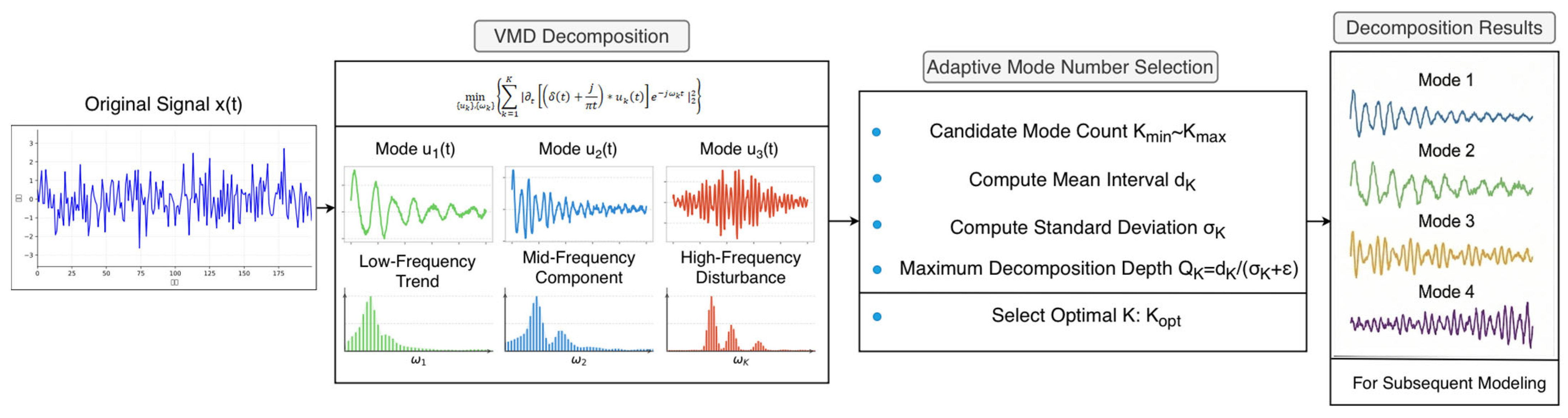
Signal decomposition and spatio-temporal learning offer two complementary routes to this problem [28,29]. VMD can separate a nonstationary signal into band-limited modes with compact spectra and strong anti-mode-mixing capability [30]. Meanwhile, graph attention mechanisms [31,32] built upon graph convolutional foundations [33] can model adaptive spatial relations among turbines or variables, and multivariate attention architectures with series-wise interaction [34,35], following the self-attention paradigm [36,37], demonstrate the value of deeper interaction between spatial structure and temporal evolution. Nevertheless, a unified interval forecasting framework that simultaneously exploits adaptive decomposition, component-wise spatio-temporal learning, and multi-quantile regression remains insufficiently developed for wind power forecasting. Different from existing interval forecasting methods, which usually perform signal decomposition, spatio-temporal feature extraction, and uncertainty estimation as separate processing stages, the proposed VSTCformer integrates adaptive decomposition, hierarchical spatio-temporal representation learning, and multi-quantile interval prediction into a unified end-to-end framework. This design enables multiscale information extraction and bidirectional space–time interaction while directly optimizing interval quality, resulting in sharper and better-calibrated prediction intervals without sacrificing point forecasting accuracy.

The main contributions of this work are summarized as follows.

(1) Adaptive decomposition. An adaptive VMD strategy is proposed to automatically determine the optimal number of decomposition modes, providing a data-adaptive multiscale representation for nonstationary wind power signals.

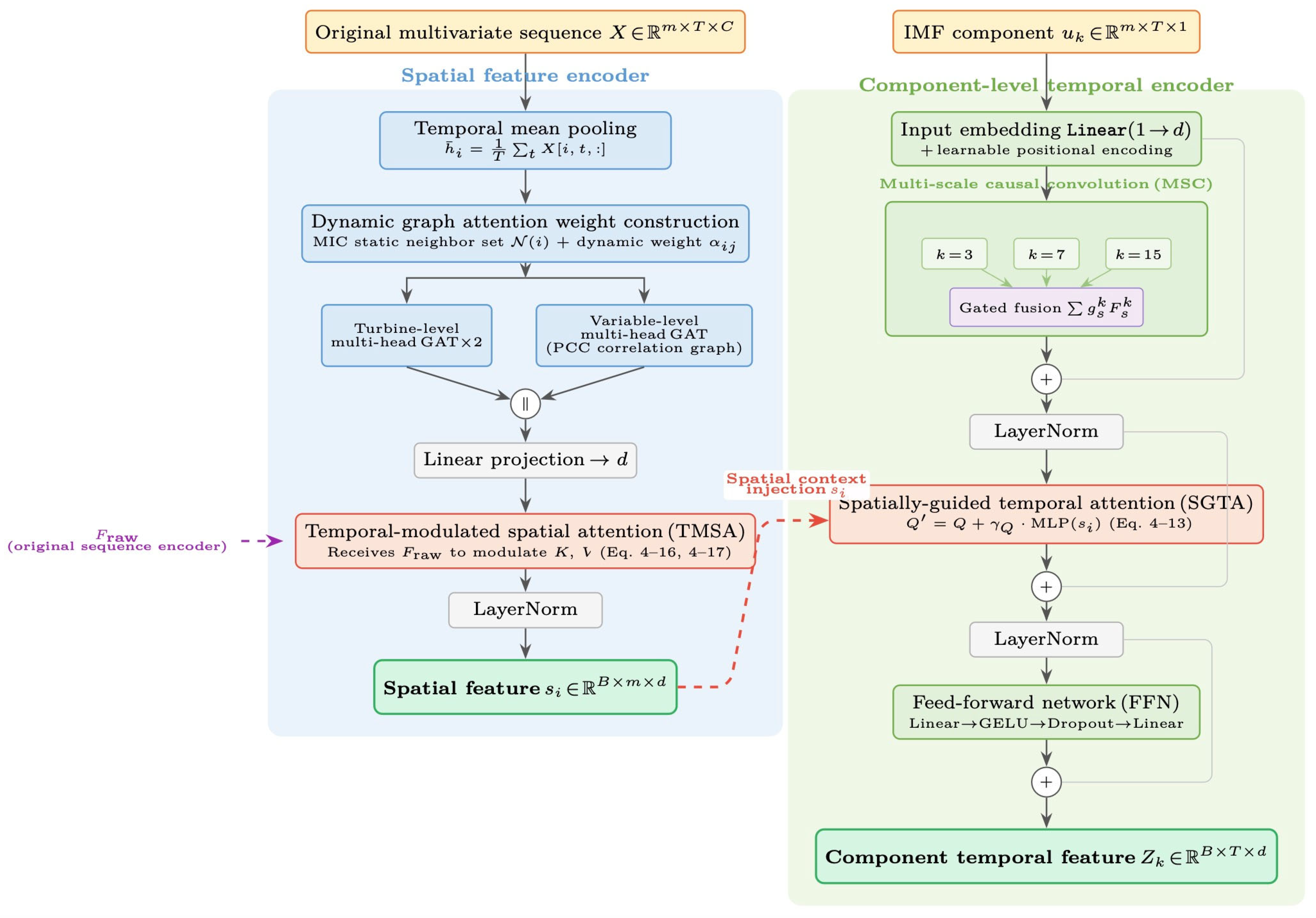
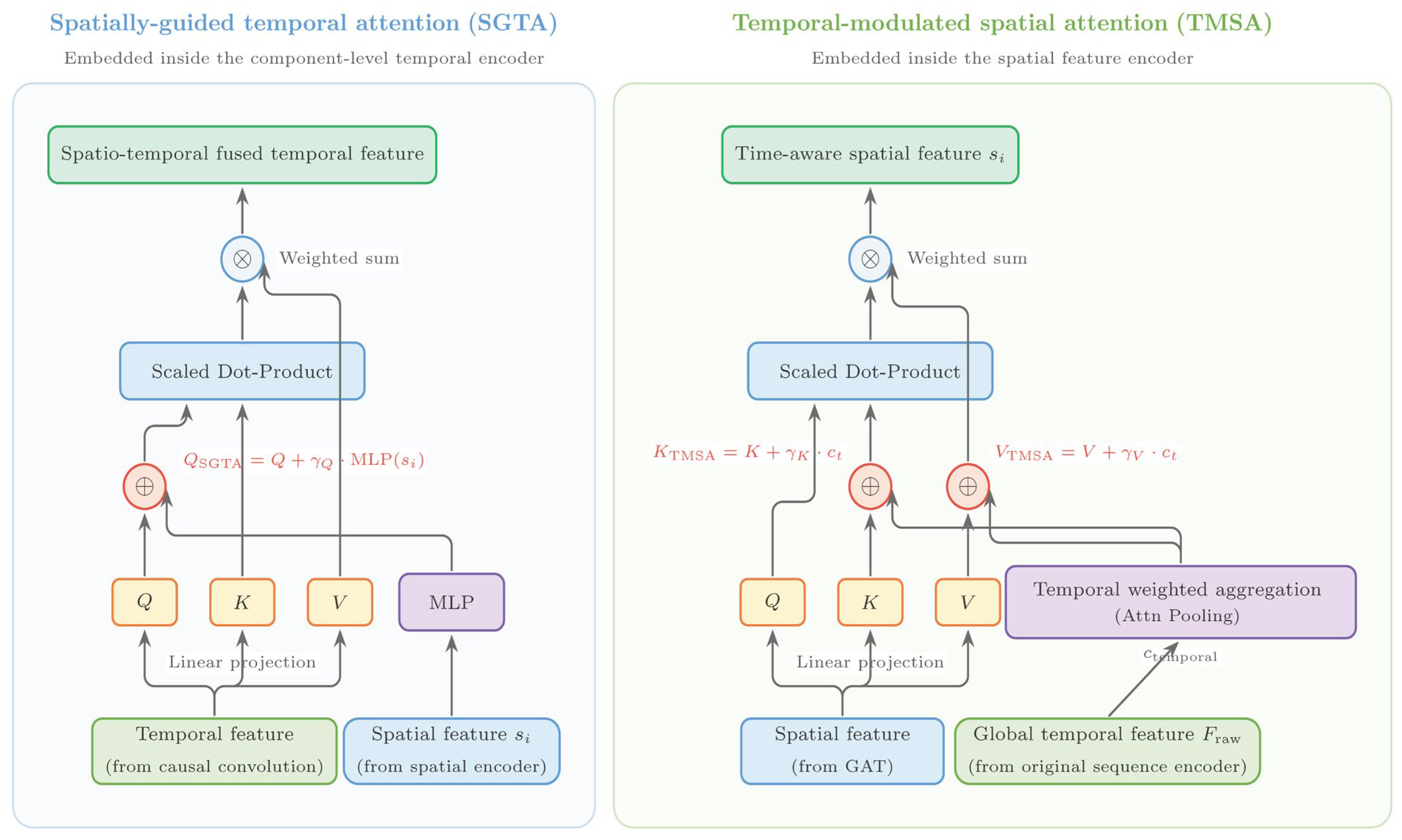
(2) Spatio-temporal representation learning. A hierarchical spatio-temporal encoding framework is developed to jointly capture global temporal information, spatial dependencies, and component-specific dynamics through cross-attention-based feature interaction.

(3) Interval forecasting. A multi-quantile regression framework is designed to directly estimate prediction intervals at multiple confidence levels, enabling accurate and well-calibrated uncertainty estimation for wind power forecasting.

2. Materials and Methods

For clarity, the VMD formulation (Equations (1)–(4)), the GAT aggregation (Equation (11)), and the pinball loss (Equations (22)–(24)) are standard and are restated only to fix notation; the novel components of this work are the adaptive mode-selection rule, the dynamic-graph construction, and the SGTA/TMSA cross-attention, whose individual contributions to the experimental results are quantified in the ablation study (Section 3.6).

2.1. Overall Framework of VSTCformer

The proposed VSTCformer follows a hierarchical “decompose-encode-fuse-regress” pipeline, as illustrated in Figure 1. Given standardized multivariate wind power sequences, the adaptive VMD module first determines the number of modes and decomposes the target power signal into K intrinsic mode functions (IMFs). Meanwhile, the original undecomposed multivariate sequence is preserved and augmented with time embedding. Based on this dual-input design, VSTCformer constructs three cooperative feature-extraction branches: a raw sequence encoder for global temporal context, a spatial feature encoder for turbine-level spatial dependency and variable-level correlation, and a component-wise temporal encoder for IMF-specific temporal evolution.

During encoding, SGTA injects spatial context into component-wise temporal modeling, whereas TMSA uses global temporal context from the raw sequence branch to modulate spatial aggregation. After this implicit spatio-temporal fusion, cross-component interaction is further performed among the decomposed IMFs, and the resulting component-fusion feature is integrated with the spatial feature and the global raw-sequence summary through three-way fusion. Finally, a multi-head quantile regression layer outputs the median forecast and a set of quantiles used to build prediction intervals. This architecture makes interval forecasting the primary objective while preserving both global sequence context and scale-specific dynamics.

2.2. Adaptive Variational Mode Decomposition

VMD is employed to separate the raw wind power sequence into band-limited components with compact spectra [30]. For a raw power sequence x(t), the decomposition seeks K intrinsic modes $u_k\left(\mathrm{t}\right)$ and their center frequencies ${\omega }_k$ by minimizing the total mode bandwidth under a reconstruction constraint. The corresponding variational problem is defined by Equations (1) and (2).

$$\underset{\left\{u_k\right\},\left\{{\omega }_k\right\}}{\mathrm{m}\mathrm{i}\mathrm{n}}\left\{{\displaystyle \sum _{k=1}^K}{∥{\mathsf{\partial }}_t\left[\left(\delta \left(t\right)+j/\pi t\right)\times u_k\left(t\right)\right]e^{-j{\omega }_{k}t}∥}_2^2\right\}$$

(1)

$${\displaystyle \sum _{k=1}^K}{u}_k\left(t\right)=x\left(t\right)$$

(2)

The optimization is solved by the alternating direction method of multipliers (ADMM) [38]. In the frequency domain, the mode and center-frequency updates used in this study are written as Equations (3) and (4).

$${\widehat{u}}_k^{\left(n+1\right)}\left(\omega \right)={\displaystyle \frac{\widehat{x}\left(\omega \right)-\sum _{i\ne k}{\widehat{u}}_i^n\left(\omega \right)+{\widehat{\lambda }}^n\left(\omega \right)/2}{1+2\alpha {\left(\omega -{\omega }_k^n\right)}^2}}$$

(3)

$${\omega }_k^{\left(n+1\right)}={\displaystyle \frac{{\int }_0^{\mathrm{\infty }}\omega {\left|{\widehat{u}}_k^{\left(n+1\right)}\left(\omega \right)\right|}^2\hspace{0.17em}d\omega }{{\int }_0^{\mathrm{\infty }}{\left|{\widehat{u}}_k^{\left(n+1\right)}\left(\omega \right)\right|}^2\hspace{0.17em}d\omega }}$$

(4)

A critical issue in VMD is the selection of the number of modes. An overly small K leaves residual high-frequency content in low-frequency modes, while an overly large K introduces pseudo-modes and unnecessary computation. To avoid manual tuning, VSTCformer uses an adaptive selection rule based on the uniformity of center-frequency spacing. For a candidate K, the mean interval, its standard deviation, and the decomposition quality score are defined by Equations (5)–(7), and the K that maximizes Q_K within [K_min, K_max] is selected.

$${\bar{d}}_K={\displaystyle \frac{1}{K-1}}{\displaystyle \sum _{k=1}^{K-1}}\left({\omega }_{k+1}-{\omega }_k\right)$$

(5)

$${\sigma }_K=\sqrt{{\displaystyle \frac{1}{K-1}}{\displaystyle \sum _{k=1}^{K-1}}{\left({\omega }_{k+1}-{\omega }_k-{\bar{d}}_K\right)}^2}$$

(6)

$$Q_K={\displaystyle \frac{{\bar{d}}_K}{{\sigma }_K+\epsilon }}$$

(7)

In the experiments, K_min = 3, K_max = 8, α = 2000, and the convergence tolerance is 10⁻⁷. After decomposition, the modes are ordered from low to high center frequency. Low-order modes mainly describe long-term trend components, whereas high-order modes contain more rapidly varying disturbances. Figure 2 shows the adaptive VMD module and the automatic mode-selection procedure. The adaptive search runs only once offline as preprocessing and does not enter the training or inference loop, so it adds a fixed one-time cost rather than a recurring one. The adaptive mode-number search introduces only a fixed preprocessing cost. In this work, only six candidate decompositions are evaluated for each dataset and forecasting horizon. After the optimal mode number is selected using only the training subset, no further candidate search is performed during model training or inference. Therefore, the online computational complexity is equivalent to that of a standard VMD-based model with a fixed mode number. To avoid information leakage, the adaptive mode selection is performed only on the training subset. Specifically, for each dataset and forecasting horizon, (Q_K) is averaged over the training input windows, and the (K) with the highest average score is selected. The selected (K) is then fixed for validation and testing. During validation and testing, VMD is applied only to the historical input window of each forecasting sample, and no future target values are used in the decomposition procedure. The objective of adaptive VMD is not to isolate sensor noise, but to separate the wind power signal into compact-band components corresponding to different temporal scales. Because VMD constrains each intrinsic mode to occupy a narrow frequency band while minimizing spectral overlap, slowly varying meteorological evolution, medium-scale periodic fluctuations, and short-term turbulent variations tend to be represented by different modes. In contrast, stochastic sensor noise usually exhibits broadband spectral characteristics without stable center frequencies, making it difficult to satisfy the compact-band constraint required for an independent mode. Consequently, random noise is mainly distributed across residual high-frequency components instead of dominating the retained intrinsic modes. In the Figure 2, low-frequency modes mainly describe meteorological evolution, medium-frequency modes represent periodic operational variations, and high-frequency modes characterize short-term turbulent fluctuations, whereas broadband stochastic noise is largely suppressed during constrained variational decomposition.

2.3. Spatial Feature Encoding and Component-Wise Temporal Encoding

VSTCformer performs differentiated encoding for the original undecomposed sequence and the decomposed IMF components shown in Figure 3. For the original multivariate sequence, time embedding is introduced and the input is processed by a raw sequence encoder and a spatial feature encoder in parallel. The raw sequence encoder preserves the global temporal context of the original sequence and provides temporal guidance for subsequent spatial modulation, while the spatial feature encoder captures turbine-level spatial relations and variable-level correlations. For each IMF, a component-wise temporal encoder is applied to preserve scale-dependent temporal dynamics through multi-scale causal convolution and gated fusion. This design separates global context preservation from component-specific evolution modeling before deeper spatio-temporal interaction.

To build a turbine-level dynamic graph, the temporal average of each turbine is first computed as in Equation (8). Pairwise attention scores and normalized edge weights are then obtained by Equations (9) and (10). The resulting attention weights are updated adaptively for each input sequence, allowing the model to capture time-varying spatial relations [39].

$${\bar{h}}_i={\displaystyle \frac{1}{T}}{\displaystyle \sum _{t=1}^T}{U}_k\left[i,t,:\right]$$

(8)

$$e_{ij}=\mathrm{L}\mathrm{e}\mathrm{a}\mathrm{k}\mathrm{y}\mathrm{R}\mathrm{e}\mathrm{L}\mathrm{U}\left({\mathbf{a}}^{\mathrm{\top }}\left[\mathbf{W}{\bar{h}}_i\hspace{0.33em}|\hspace{0.33em}\mathbf{W}{\bar{h}}_j\right]\right)$$

(9)

$${\alpha }_{ij}={\displaystyle \frac{\mathrm{e}\mathrm{x}\mathrm{p}\left(e_{ij}\right)}{\sum _{j^{\prime }\in \mathcal{N}\left(i\right)}\mathrm{e}\mathrm{x}\mathrm{p}\left(e_{i{j}^{\prime }}\right)}}$$

(10)

On the resulting graph, graph attention networks (GATs) are used for feature aggregation [31]. The node update rule is expressed by Equation (11). A variable-level correlation graph is constructed in parallel using the Pearson correlation coefficient so that cross-variable dependencies can also be modeled in the spatial encoding branch of the original multivariate sequence.

$$h_i^{\left(l+1\right)}=\sigma \left(\sum _{j\in \mathcal{N}\left(i\right)}{\alpha }_{ij}^{\left(l\right)}{\mathbf{W}}^{\left(l\right)}{h}_j^{\left(l\right)}\right)$$

(11)

For temporal dynamics, three parallel causal convolution branches with kernel sizes 3, 7, and 15 are used to capture short-, medium-, and long-range variations. Their outputs are fused through learnable gates as in Equation (12). Inspired by gated convolutional design [40] and its modern extensions to general time-series analysis [41], this mechanism assigns different scale weights to different modes, so low-frequency components can emphasize long-range patterns while high-frequency modes remain sensitive to fast fluctuations. Together, these branches provide the spatial features, global temporal context, and component-specific temporal representations required for the subsequent cross-attention and three-way fusion stages.

$$F_{\mathrm{time}}^k={\displaystyle \sum _{s=1}^3}{g}_s^k\cdot F_s^k$$

(12)

2.4. Spatio-Temporal Cross-Attention Fusion

After branch-wise encoding, VSTCformer performs hierarchical fusion through a spatio-temporal cross-attention module [42,43,44], shown in Figure 4. The design contains two complementary branches: SGTA and TMSA. Rather than acting only as a post-hoc fusion block, these two mechanisms are embedded into different encoding pathways to realize implicit spatio-temporal fusion during feature extraction. SGTA injects spatial context from the spatial feature encoder into the component-wise temporal encoding process, while TMSA uses temporal context from the raw sequence encoder to modulate spatial aggregation.

For SGTA, a global spatial context vector is first computed from the encoded component features $H\in R^{m\times T\times d}$, as shown in Equation (13). The temporal query is then modulated by this context according to Equation (14), following the conditioning idea of feature-wise linear modulation (FiLM) [45]. The resulting temporal attention is given by Equation (15).

$$c_{\mathrm{spatial}}={\displaystyle \frac{1}{m}}{\displaystyle \sum _{i=1}^m}\mathrm{M}\mathrm{L}\mathrm{P}\left(H\left[i,:,:\right]\right)$$

(13)

$$Q_{\mathrm{SGTA}}=Q+{\gamma }_Q\cdot c_{\mathrm{spatial}}$$

(14)

$$\mathrm{S}\mathrm{G}\mathrm{T}\mathrm{A}\left(Q,K,V\right)=\mathrm{S}\mathrm{o}\mathrm{f}\mathrm{t}\mathrm{m}\mathrm{a}\mathrm{x}\left({\displaystyle \frac{Q_{\mathrm{SGTA}}{K}^{\mathrm{\top }}}{\sqrt{d_k}}}\right)V$$

(15)

For TMSA, the temporal context is summarized through weighted aggregation over time, as in Equation (16). This context is used to modulate the key and value tensors according to Equations (17) and (18), and the resulting spatial attention is defined by Equation (19).

$$c_{\mathrm{temporal}}={\displaystyle \sum _{t=1}^T}{w}_t\cdot H\left[:,t,:\right]$$

(16)

$$K_{\mathrm{TMSA}}=K+{\gamma }_K\cdot c_{\mathrm{temporal}}$$

(17)

$$V_{\mathrm{TMSA}}=V+{\gamma }_V\cdot c_{\mathrm{temporal}}$$

(18)

$$\mathrm{T}\mathrm{M}\mathrm{S}\mathrm{A}\left(Q,K,V\right)=\mathrm{S}\mathrm{o}\mathrm{f}\mathrm{t}\mathrm{m}\mathrm{a}\mathrm{x}\left({\displaystyle \frac{Q{\left(K_{\mathrm{TMSA}}\right)}^{\mathrm{\top }}}{\sqrt{d_k}}}\right)V_{\mathrm{TMSA}}$$

(19)

Beyond within-branch fusion, VSTCformer also performs explicit post-encoding integration. Cross-scale dependency is modeled through inter-component interaction, which allows low-frequency trend information and high-frequency fluctuation information to be exchanged across decomposed modes. After cross-component interaction, the resulting component embeddings are aggregated into a unified component-fusion representation. This representation is then further combined with the spatial feature encoder output and the global summary generated by the raw sequence encoder through three-way fusion, producing the final fused representation for subsequent quantile prediction.

$$Z_k^{\mathrm{inter}}=Z_k+\sum _{j\ne k}{\beta }_{kj}\cdot \mathrm{C}\mathrm{r}\mathrm{o}\mathrm{s}\mathrm{s}\mathrm{A}\mathrm{t}\mathrm{t}\mathrm{n}\left(Z_k,Z_j,Z_j\right)$$

(20)

$$Z_{\mathrm{fused}}={\displaystyle \sum _{k=1}^K}{\lambda }_k\cdot Z_k^{\mathrm{inter}}$$

(21)

2.5. Multi-Quantile Regression for Interval Prediction

To generate interval forecasts, VSTCformer uses a multi-quantile regression head based on quantile regression [15]. Nine quantiles are jointly predicted, namely τ ∈ {0.05, 0.10, 0.25, 0.40, 0.50, 0.60, 0.75, 0.90, 0.95}. The median forecast (τ = 0.50) is used as the point estimate, the interval [0.05, 0.95] forms the 90% prediction interval, and [0.10, 0.90] forms the 80% interval.

Each quantile is produced by an independent multilayer perceptron branch that shares the fused spatio-temporal representation. The quantile output is expressed by Equation (22), and the pinball loss for an individual quantile is defined by Equation (23). The overall training objective is the weighted sum shown in Equation (24).

$${\widehat{y}}_{\tau }={\mathrm{M}\mathrm{L}\mathrm{P}}_{\tau }\left(Z_{\mathrm{fused}}\right)$$

(22)

$$L_{\tau }\left(y,{\widehat{y}}_{\tau }\right)=\left\{\begin{array}{ll}\tau \left(y-{\widehat{y}}_{\tau }\right),& \mathrm{if} y\ge {\widehat{y}}_{\tau }\\ \left(1-\tau \right)\left({\widehat{y}}_{\tau }-y\right),& \mathrm{if} y<{\widehat{y}}_{\tau }\end{array}\right.$$

(23)

$$L_{\mathrm{total}}=\sum _{\tau }{w}_{\tau }\hspace{0.33em}{L}_{\tau }\left(y,{\widehat{y}}_{\tau }\right)$$

(24)

Because independently estimated quantiles may occasionally cross, isotonic regression is applied during inference when necessary to restore monotonicity [46]. In this way, the model produces a coherent set of predictive quantiles that can be directly converted into interval forecasts, while the median quantile is simultaneously used as an auxiliary point estimate of the conditional distribution center. Because all quantile branches share the same backbone representation and are jointly optimized under the combined pinball loss, quantile crossing is rarely observed in practice. Instead of introducing additional monotonicity constraints during training, which increase optimization complexity and may restrict the flexibility of individual quantile estimation, isotonic regression is adopted as a lightweight safeguard during inference. In our experiments, fewer than 2% of the test samples require monotonic correction, indicating that quantile crossing has only a negligible impact on the overall prediction performance.

3. Experiments and Results

3.1. Datasets, Preprocessing, and Evaluation Metrics

The experiments use two public benchmarks: SDWPF (Spatial Dynamic Wind Power Forecasting) [47] and GEFCom2012 (Global Energy Forecasting Competition 2012) [48]. SDWPF contains 10 min operating records from 134 turbines over 245 days. Following the thesis setting, 10 representative turbines were selected, providing approximately 35,000 valid samples per turbine. GEFCom2012 provides hourly normalized power data from seven wind farms between 2009 and 2012. The two datasets differ in spatial scale, temporal resolution, and volatility, which allows the robustness of interval forecasting to be assessed under distinct operating regimes.

For SDWPF, abnormal records were screened using physical constraints, including negative power values, zero power under wind speeds above 2.5 m/s, blade pitch angles above 89°, and invalid wind-direction or yaw ranges. Abnormal values were imputed by backward-forward filling. Calendar features were extracted from the timestamp, and all inputs were standardized using statistics from the training set. For GEFCom2012, turbine-level operational variables are unavailable, so only normalized calendar features were used. Different from the point-forecasting setup, wavelet denoising was not applied here; the raw power sequence was directly fed to the adaptive VMD module so that decomposition and denoising were handled in a unified way.

Because VSTCformer outputs both central and interval forecasts, evaluation was conducted from two perspectives. The median forecast (τ = 0.50) was evaluated using mean squared error (MSE), mean absolute error (MAE), and root mean square error (RMSE). Interval quality was evaluated using prediction interval coverage probability (PICP), prediction interval normalized average width (PINAW), and coverage width-based criterion (CWC) [27]. Their definitions are given by Equations (25)–(27), where $L_i$ and $U_i$ are the lower and upper interval bounds, R is the range of the target variable, and μ is the nominal coverage rate.

$$\mathrm{P}\mathrm{I}\mathrm{C}\mathrm{P}={\displaystyle \frac{1}{N}}{\displaystyle \sum _{i=1}^N}\mathbf{1}\{L_i\le y_i\le U_i\}$$

(25)

$$\mathrm{P}\mathrm{I}\mathrm{N}\mathrm{A}\mathrm{W}={\displaystyle \frac{1}{N\cdot R}}{\displaystyle \sum _{i=1}^N}\left(U_i-L_i\right)$$

(26)

$$\mathrm{W}\mathrm{C}=\mathrm{P}\mathrm{I}\mathrm{N}\mathrm{A}\mathrm{W}\cdot \left[1+\gamma \cdot \mathrm{e}\mathrm{x}\mathrm{p}\left(-\eta \left(\mathrm{P}\mathrm{I}\mathrm{C}\mathrm{P}-\mu \right)\right)\right]$$

(27)

3.2. Experimental Settings

Main experimental settings for VSTCformer is shown in

Table 1. Main experimental settings for VSTCformer.

Item	Setting
Forecasting horizons	6 h, 12 h, 24 h
Input length	Twice the prediction horizon
Data split	Training/validation/test = 7:1:2
Adaptive VMD candidate range	K ∈ [3, 8]
VMD penalty factor	α = 2000
Graph attention configuration	4 heads; hidden dimension 128
Cross-attention configuration	8 heads
Quantile branch	Two-layer MLP; hidden dimension 256
Optimizer and scheduler	Adam; cosine annealing with warm restarts
Maximum epochs/batch size	50/16
Early stopping patience	5 epochs
Signal preprocessing	Raw power sequence directly decomposed by adaptive VMD

. The forecasting horizons were set to 6 h, 12 h, and 24 h. The input sequence length was fixed to twice the prediction horizon. Both datasets were divided into training, validation, and test subsets using a 7:1:2 ratio. For SDWPF, the three horizons correspond to 36, 72, and 144 steps under the 10 min resolution. For GEFCom2012, they correspond to 12, 24, and 48 steps under the hourly resolution.

In VSTCformer, the candidate range of the adaptive VMD module was set to [3, 8], and the penalty factor α was fixed to 2000. The spatial encoder used four graph-attention heads with a hidden dimension of 128 per head, the raw-sequence encoder and component-wise temporal encoder used the same hidden dimension, and the spatio-temporal cross-attention block used eight attention heads. Each quantile branch contained two fully connected layers with a hidden dimension of 256. Adam was adopted as the optimizer, the initial learning rate was 1 × 10⁻⁴, and cosine annealing [49] was used for learning-rate scheduling. The maximum number of epochs was 50, the batch size was 16, and early stopping with a patience of five epochs was applied. All reported metrics are averaged over five independent runs with different random seeds to reduce the influence of random initialization. Selected mode numbers of adaptive VMD under the leakage-free training-only selection protocol. The mode-number search was conducted using only the training subset. The validation and test subsets used the selected (K) without re-estimating the candidate range or accessing future observations. For point forecasting, the compared baselines included LSTM [50], GRU [51], TCN [52], DLinear [53], Transformer [37], Informer [54], PatchTST [55], iTransformer [56], TimeXer [57], STGCN [58], DCRNN [59], and GSTAformer [60], a deterministic point-forecasting model previously proposed by the present authors. For interval forecasting, the compared baselines included LSTM-QR, GRU-QR, TCN-QR, Transformer-QR, STGCN-QR, DCRNN-QR, MC-Dropout [61], Deep Ensembles [62], and BNN [63]. The QR-suffixed variants attach the same multi-quantile regression head used in VSTCformer to each backbone.

3.3. Auxiliary Point Forecasting Performance

Although interval prediction is the primary objective of this work, the accuracy of the median forecast is also reported to evaluate how well the model captures the conditional distribution center.

Table 2. Point forecasting performance on the SDWPF dataset.

Model	6 h			12 h			24 h
	MSE	MAE	RMSE	MSE	MAE	RMSE	MSE	MAE	RMSE
LSTM [50]	0.4253	0.4285	0.6521	0.6907	0.5858	0.8308	0.8789	0.6999	0.9375
GRU [51]	0.4070	0.4213	0.6379	0.6538	0.5832	0.8086	0.8866	0.7100	0.9415
TCN [52]	0.4096	0.4408	0.6400	0.6344	0.5773	0.7964	0.8657	0.6896	0.9304
DLinear [53]	0.4210	0.4779	0.6488	0.6434	0.6121	0.8021	0.8462	0.7298	0.9199
Transformer [37]	0.4933	0.4609	0.7009	0.8826	0.6503	0.9390	1.2029	0.7949	1.0938
Informer [54]	0.5179	0.4759	0.7192	0.8135	0.6254	0.9018	1.1274	0.7595	1.0583
PatchTST [55]	0.4123	0.3983	0.6420	0.7361	0.5888	0.8579	1.0648	0.7249	1.0303
iTransformer [56]	0.4574	0.4204	0.6762	0.7796	0.5835	0.8828	1.1849	0.7480	1.0867
TimeXer [57]	0.4555	0.4259	0.6747	0.7488	0.5844	0.8653	1.0731	0.7216	1.0344
STGCN [58]	0.3968	0.4256	0.6299	0.5923	0.5612	0.7696	0.8124	0.6708	0.9013
DCRNN [59]	0.4015	0.4278	0.6336	0.6087	0.5689	0.7802	0.8267	0.6785	0.9092
GSTAformer [60]	0.3887	0.4210	0.6234	0.5469	0.5364	0.7395	0.7480	0.6362	0.8648
VSTCformer	0.3864	0.4192	0.6219	0.5452	0.5379	0.7382	0.7493	0.6352	0.8655

and

Table 3. Point forecasting performance on the GEFCom2012 dataset.

Model	6 h			12 h			24 h
	MSE	MAE	RMSE	MSE	MAE	RMSE	MSE	MAE	RMSE
LSTM [50]	0.3294	0.3413	0.5740	0.4177	0.3913	0.6463	0.4910	0.4292	0.7007
GRU [51]	0.3401	0.3509	0.5832	0.4201	0.3910	0.6481	0.4943	0.4310	0.7031
TCN [52]	0.3359	0.3523	0.5795	0.4148	0.3940	0.6440	0.5091	0.4509	0.7135
DLinear [53]	0.3106	0.3205	0.5572	0.4037	0.3712	0.6353	0.5227	0.4552	0.7230
Transformer [37]	0.2780	0.2760	0.5266	0.3984	0.3377	0.6303	0.5389	0.4354	0.7336
Informer [54]	0.2988	0.3017	0.5462	0.4113	0.3670	0.6399	0.5332	0.4571	0.7298
PatchTST [55]	0.2332	0.2310	0.4828	0.3478	0.3239	0.5897	0.4406	0.4017	0.6636
iTransformer [56]	0.2327	0.2306	0.4823	0.3330	0.3282	0.5769	0.4747	0.3925	0.6890
TimeXer [57]	0.2176	0.2303	0.4665	0.3431	0.3260	0.5856	0.4522	0.4104	0.6724
STGCN [58]	0.2243	0.2345	0.4736	0.3312	0.3298	0.5755	0.4367	0.4012	0.6608
DCRNN [59]	0.2298	0.2376	0.4794	0.3389	0.3345	0.5822	0.4435	0.4056	0.6659
GSTAformer [60]	0.1958	0.2297	0.4425	0.3080	0.3207	0.5549	0.4001	0.3799	0.6325
VSTCformer	0.1939	0.2304	0.4403	0.3067	0.3212	0.5538	0.4023	0.3778	0.6343

compare VSTCformer with 12 representative baselines on SDWPF and GEFCom2012, respectively.

On SDWPF, VSTCformer and GSTAformer form the leading performance tier, followed by STGCN and DCRNN, while the purely temporal baselines remain clearly behind. VSTCformer achieves the lowest MSE at 6 h (0.3864) and 12 h (0.5452), outperforming GSTAformer by 0.59% and 0.31%, respectively. At 24 h, the two models are nearly tied (0.7493 versus 0.7480), which indicates that the proposed architecture preserves point-forecast accuracy while prioritizing uncertainty modeling. Compared with STGCN, the 24 h MSE is reduced from 0.8124 to 0.7493, highlighting the advantage of combining adaptive decomposition with dynamic spatio-temporal interaction rather than relying on a fixed graph.

Table 3 reports the corresponding results on GEFCom2012. Because this dataset is smoother and more periodic than SDWPF, all models achieve lower absolute errors, and Transformer-based baselines such as TimeXer, iTransformer, and PatchTST become more competitive. Even so, VSTCformer still obtains the lowest MSE at 6 h and 12 h and remains comparable to GSTAformer at 24 h.

Specifically, VSTCformer reaches MSE values of 0.1939 and 0.3067 at 6 h and 12 h, improving on GSTAformer by 0.97% and 0.42%, respectively. At 24 h, the two models again show nearly identical performance (0.4023 versus 0.4001), while VSTCformer yields a slightly lower MAE. Taken together, the results on both datasets indicate that the proposed interval-forecasting framework does not sacrifice central-estimation quality and retains strong generalization across different temporal resolutions and operating regimes.

3.4. Interval Forecasting Performance

Table 4. Interval forecasting performance on the SDWPF dataset (90% prediction interval).

Model	6 h			12 h			24 h
	PICP	PINAW	CWC	PICP	PINAW	CWC	PICP	PINAW	CWC
LSTM-QR	0.882	0.353	0.777	0.867	0.507	1.213	0.782	0.427	1.820
GRU-QR	0.874	0.328	0.741	0.903	0.519	0.519	0.819	0.520	1.685
TCN-QR	0.913	0.443	0.443	0.806	0.572	2.044	0.735	0.421	2.608
Transformer-QR	0.907	0.433	0.433	0.834	0.627	1.841	0.756	0.424	2.210
STGCN-QR	0.906	0.365	0.365	0.883	0.436	0.851	0.852	0.398	0.952
DCRNN-QR	0.901	0.371	0.371	0.879	0.452	0.973	0.840	0.410	1.086
MC-Dropout [61]	0.921	0.410	0.410	0.876	0.544	1.356	0.801	0.486	1.674
Deep Ensembles [62]	0.919	0.386	0.386	0.892	0.473	0.824	0.844	0.451	1.165
BNN [63]	0.896	0.398	0.512	0.851	0.523	1.503	0.793	0.468	1.894
VSTCformer	0.908	0.328	0.328	0.899	0.309	0.619	0.890	0.324	0.681

and

Table 5. Interval forecasting performance on the GEFCom2012 dataset (90% prediction interval).

Model	6 h			12 h			24 h
	PICP	PINAW	CWC	PICP	PINAW	CWC	PICP	PINAW	CWC
LSTM-QR	0.953	0.360	0.360	0.946	0.412	0.412	0.957	0.453	0.453
GRU-QR	0.949	0.341	0.341	0.950	0.410	0.410	0.937	0.450	0.450
Transformer-QR	0.952	0.375	0.375	0.958	0.421	0.421	0.960	0.451	0.451
TCN-QR	0.919	0.378	0.378	0.925	0.427	0.427	0.946	0.489	0.489
STGCN-QR	0.923	0.353	0.353	0.916	0.398	0.398	0.928	0.435	0.435
DCRNN-QR	0.919	0.359	0.359	0.912	0.403	0.403	0.925	0.439	0.439
MC-Dropout [61]	0.946	0.382	0.382	0.939	0.435	0.435	0.948	0.471	0.471
Deep Ensembles [62]	0.951	0.365	0.365	0.943	0.418	0.418	0.952	0.442	0.442
BNN [63]	0.935	0.391	0.391	0.928	0.446	0.446	0.931	0.468	0.468
VSTCformer	0.901	0.333	0.333	0.894	0.368	0.814	0.913	0.410	0.410

compare the 90% interval forecasting performance on SDWPF and GEFCom2012, respectively. Across both datasets, VSTCformer consistently yields the narrowest intervals and the strongest overall coverage-width trade-off.

On SDWPF, VSTCformer keeps PICP close to the nominal 90% target at all horizons, with values of 0.908, 0.899, and 0.890 for 6 h, 12 h, and 24 h, respectively. At 6 h, it slightly exceeds the nominal coverage while reducing PINAW to 0.328, outperforming the strongest graph-based baselines STGCN-QR and DCRNN-QR. At 12 h, its PICP falls only marginally below the nominal rate, but its PINAW remains the narrowest among all methods at 0.309. The advantage becomes especially clear at 24 h. VSTCformer achieves the lowest PINAW (0.324) and the best CWC (0.681), improving on STGCN-QR by about 18.6% in PINAW and 28.5% in CWC. These results indicate that adaptive VMD and spatio-temporal cross-attention help the model maintain informative and well-calibrated intervals even under long-horizon uncertainty accumulation.

Table 5 further reports the interval forecasting results on GEFCom2012. Because this dataset is smoother and more periodic, many baselines tend to achieve high or even over-conservative coverage, but they often do so by widening the interval excessively.

VSTCformer again produces the narrowest intervals at all horizons, with PINAW values of 0.333, 0.368, and 0.410 for 6 h, 12 h, and 24 h, respectively. At 6 h, it achieves both the best CWC and an almost ideal PICP of 0.901. At 12 h, the PICP is 0.894, only slightly below the nominal level, yet the interval remains substantially sharper than those of STGCN-QR and DCRNN-QR.

At 24 h, VSTCformer raises PICP to 0.913 and obtains the lowest CWC of 0.410, outperforming all competing methods on the overall coverage-width trade-off. Together with the SDWPF results, these findings show that the proposed framework generalizes well across datasets with markedly different volatility patterns and that its main strength lies in delivering sharp intervals without giving up calibration.

Although VSTCformer generally produces narrower prediction intervals than competing methods, these improvements are not obtained by substantially reducing coverage. Across both datasets, the achieved PICP remains close to the nominal confidence level, while the corresponding CWC consistently ranks among the best. Since CWC imposes an exponential penalty whenever coverage falls below the nominal level, the superior CWC values indicate a favorable balance between interval sharpness and calibration rather than overconfident uncertainty estimation.

3.5. Visualization of Prediction Intervals

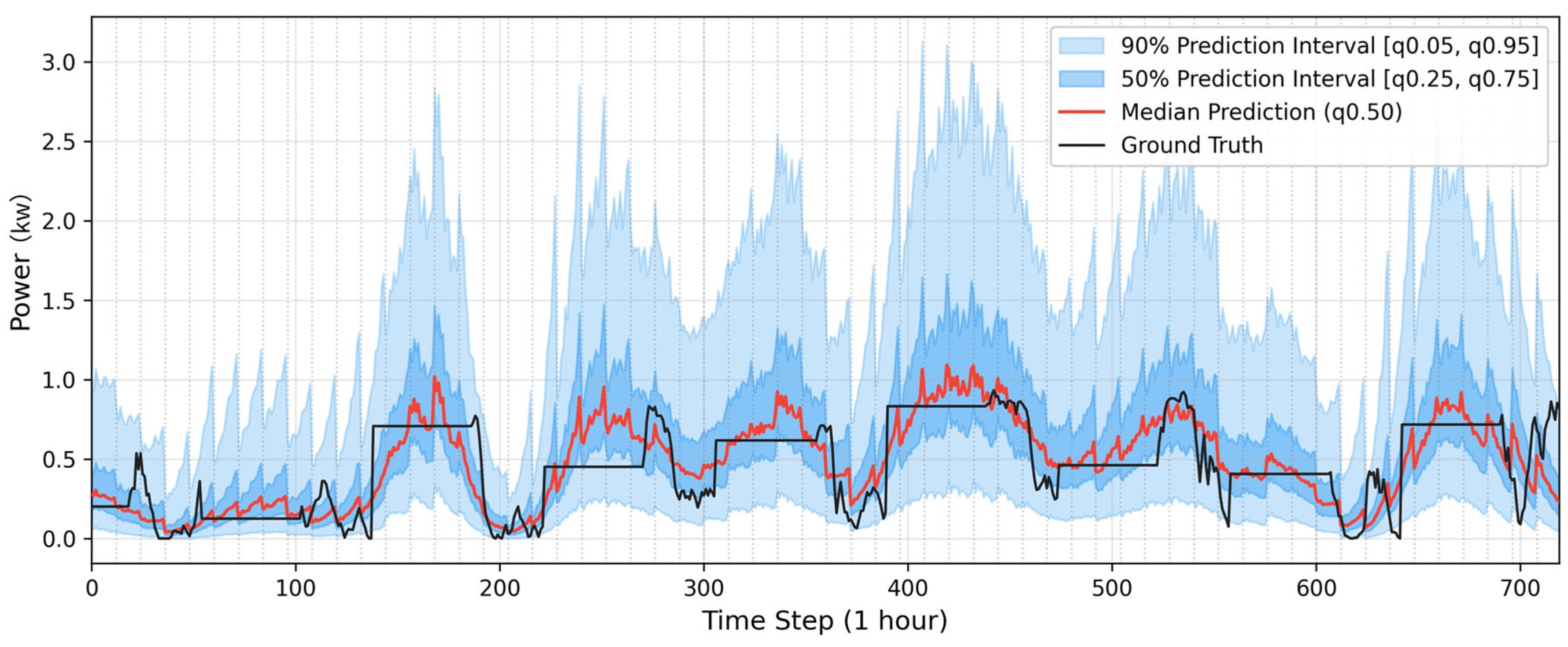
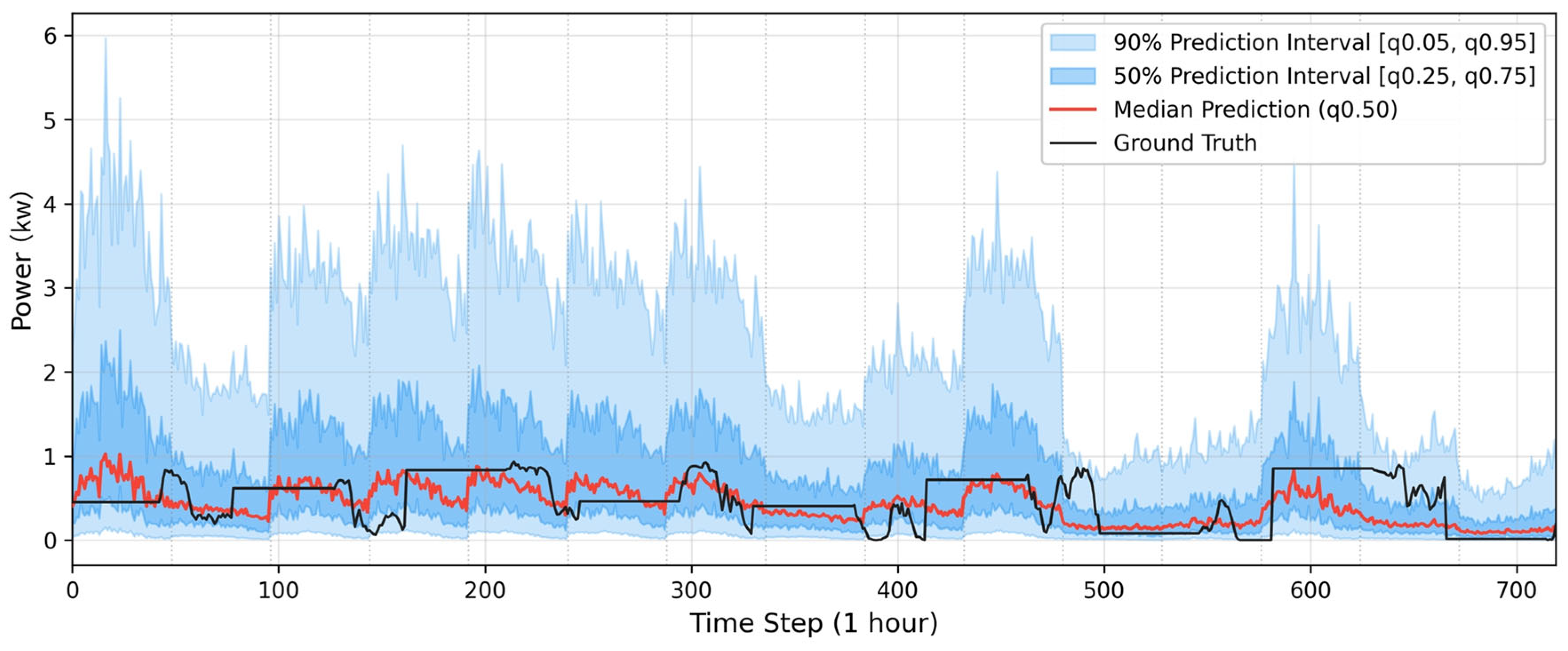
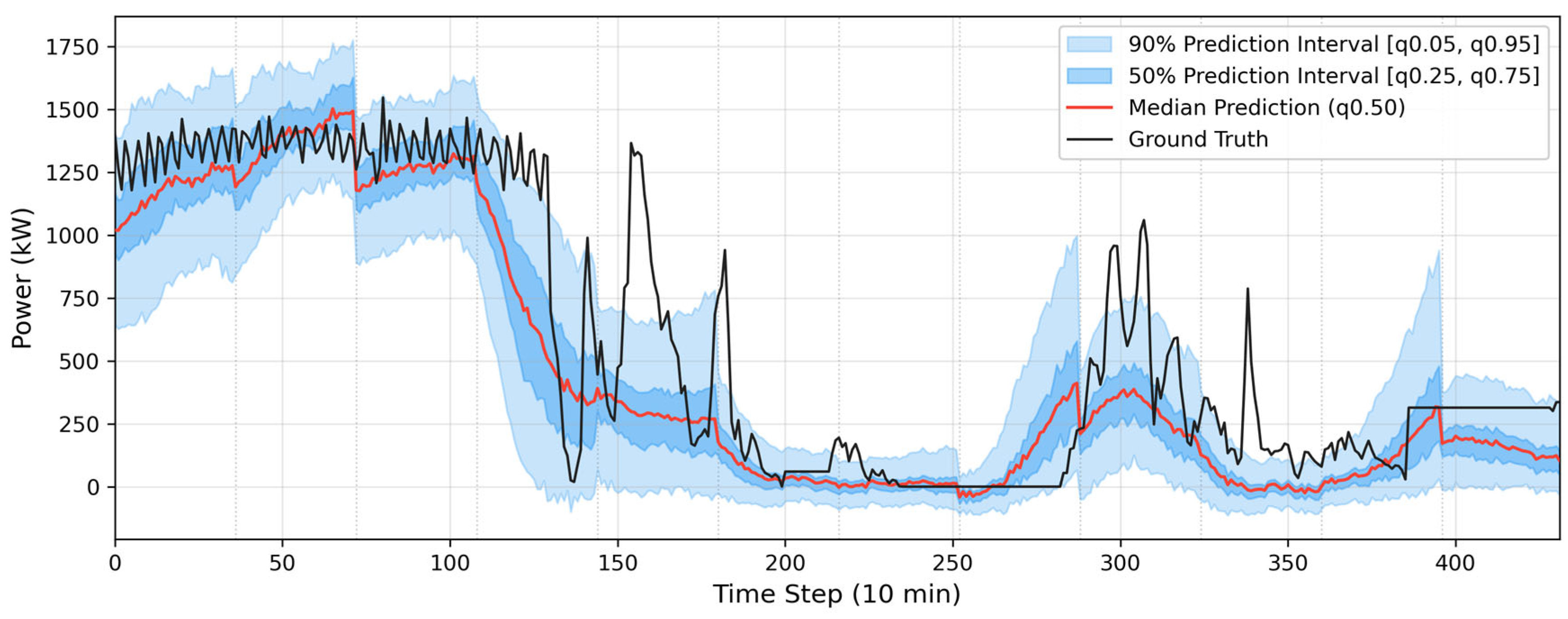
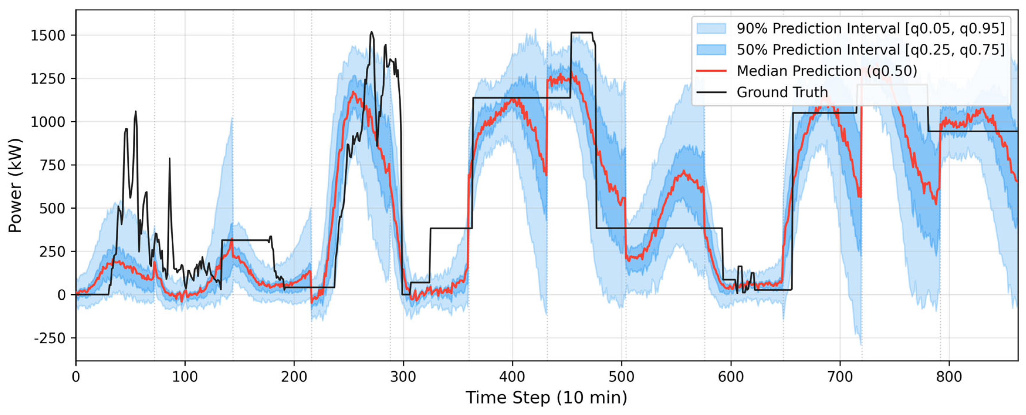
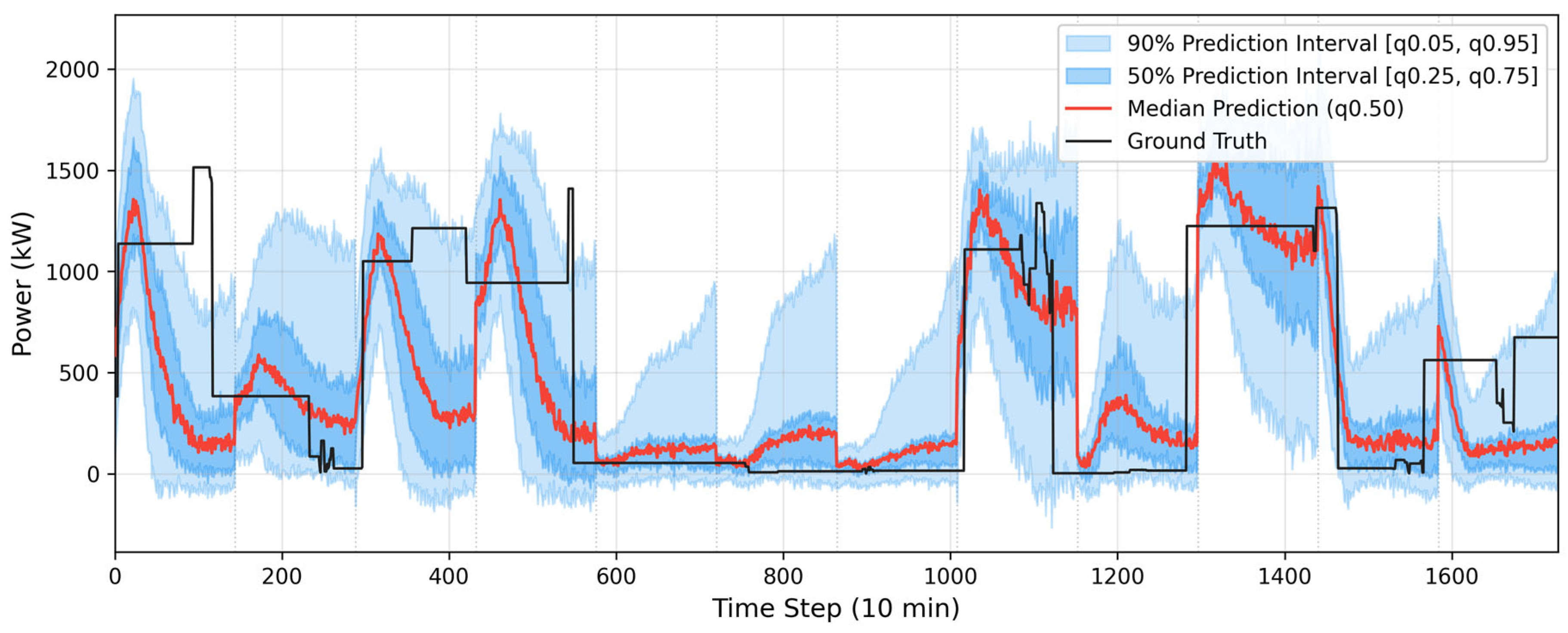
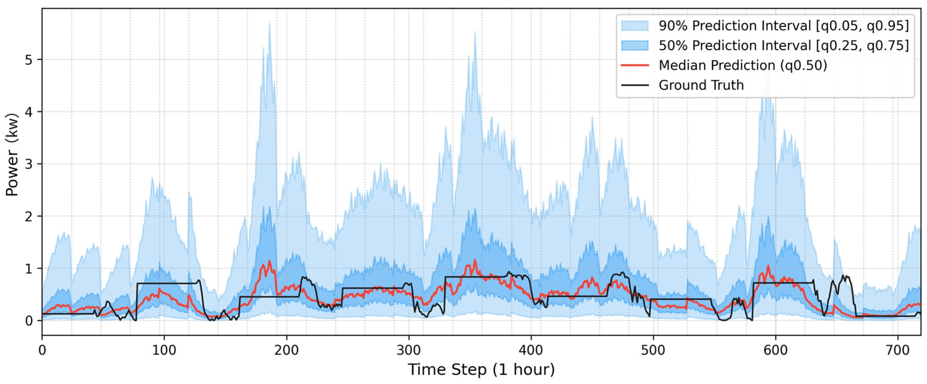
Figure 5, Figure 6, Figure 7, Figure 8, Figure 9 and Figure 10 visualize the interval forecasts on SDWPF (Figure 5, Figure 6 and Figure 7) and GEFCom2012 (Figure 8, Figure 9 and Figure 10) for the 6 h, 12 h, and 24 h horizons. On both datasets VSTCformer characterizes the stochastic fluctuation of the power sequence and its uncertainty well: most observations fall within the 90% prediction interval and tend to lie close to the 50% interval, indicating good coverage and quantile-description capability, and the 6 h forecast is the most accurate, with the median curve closest to the ground truth. As the horizon extends to 12 h and 24 h, the median fit to local extrema weakens and the intervals gradually widen, but this widening is concentrated around rapid ramps, sharp drops, and short-term oscillations, while the intervals remain compact during stable periods, reflecting the model’s adaptive behaviour. The two datasets nonetheless show distinct visual characteristics. Because SDWPF is highly stochastic, the model’s strength lies in tracking strong random fluctuations; on GEFCom2012, which has lower overall volatility and stronger periodicity, the advantage instead appears in the fine description of stable stages, where the 50% interval stays compact and the median curve remains consistent with the ground truth over most periodic segments. On GEFCom2012 the interval expansion at the longer horizons is mainly confined to periodic peak–valley transitions and phases of increased volatility, with many stable segments still kept narrow, showing that VSTCformer balances coverage and informativeness well on both datasets. The two benchmarks represent different stationarity regimes, with SDWPF exhibiting highly nonstationary and volatile characteristics, whereas GEFCom2012 is comparatively smoother and more periodic. These results indicate that VSTCformer is applicable under different stationarity conditions. For highly nonstationary series, adaptive VMD effectively separates mixed-frequency components, enabling more accurate spatio-temporal representation learning. For smoother series, the adaptive mode-selection strategy typically identifies fewer effective modes, allowing VMD to function primarily as a multiscale feature extraction mechanism while avoiding unnecessary decomposition. Therefore, the proposed framework can maintain robust interval forecasting performance across datasets with different statistical characteristics.

3.6. Ablation Study

To quantify the contributions of the key components in VSTCformer, an ablation study was performed on SDWPF for the 24 h horizon, shown in

Table 6. Ablation results of VSTCformer on SDWPF for the 24 h horizon.

Variant	MSE	MAE	RMSE	PICP	PINAW	CWC
w/o VMD	0.761	0.648	0.873	0.879	0.346	0.772
w/o SGTA	0.753	0.641	0.868	0.886	0.335	0.721
w/o TMSA	0.756	0.642	0.869	0.883	0.338	0.737
w/o Inter-IMF	0.758	0.645	0.871	0.881	0.340	0.751
w/o GAT	0.752	0.640	0.867	0.887	0.331	0.710
VSTCformer	0.749	0.635	0.866	0.890	0.324	0.681

. The evaluated variants remove the adaptive VMD module, SGTA, TMSA, inter-IMF interaction, or the dynamic GAT-based spatial encoder.

From the point-forecasting perspective, removing VMD produces the largest MSE increase, from 0.749 to 0.761, confirming the importance of decomposition for simplifying the nonstationary signal. Removing inter-IMF interaction, TMSA, SGTA, or GAT also degrades performance, with TMSA causing a slightly larger loss than SGTA. Although removing the GAT changes MSE only marginally (0.749 to 0.752), it raises CWC from 0.681 to 0.710 (~4.2%); the dynamic graph therefore mainly improves interval sharpness rather than point accuracy. Although the removal of the dynamic graph causes only a marginal increase in point forecasting error, its influence on interval quality is considerably more pronounced. This behavior is consistent with the design objective of the graph module, which aims to improve spatial dependency modeling for uncertainty estimation rather than deterministic prediction. The increased CWC indicates that the graph contributes primarily to producing sharper and better-calibrated prediction intervals. From the interval-forecasting perspective, the impact is even more pronounced: without VMD, PICP drops from 0.890 to 0.879, PINAW rises from 0.324 to 0.346, and CWC increases from 0.681 to 0.772. Overall, the ablation results verify that adaptive VMD, inter-IMF interaction, TMSA, SGTA, and dynamic graph attention all make indispensable contributions to the final coverage-width balance.

4. Discussion

The updated experiments show that the main advantage of VSTCformer is not a dramatic improvement in point accuracy over the strongest deterministic competitor, but a substantial enhancement in uncertainty quantification while preserving competitive median forecasts. This aligns with the broader observation in the probabilistic forecasting literature [5,64] that decomposition-based preprocessing can significantly tighten predictive intervals when combined with distributional learning objectives. Across both SDWPF and GEFCom2012, the model consistently generates the narrowest prediction intervals, and in four of the six interval-evaluation settings it also achieves the best CWC. Even in the remaining two settings, the CWC penalty is mainly caused by a marginal shortfall of PICP relative to the nominal 90% target rather than by overconfidently narrow intervals.

The ablation study clarifies why this behavior emerges. Adaptive VMD is the most influential module because it separates the raw sequence into components with more regular spectral structure, making both temporal extrapolation and uncertainty estimation easier. SGTA and TMSA provide complementary benefits by enabling bidirectional coupling between spatial topology and temporal evolution, while inter-IMF interaction prevents scale isolation. The slightly larger degradation caused by removing TMSA than by removing SGTA suggests that dynamically modulating spatial aggregation according to temporal context is particularly important for long-horizon forecasting. The current dynamic graph models statistical spatial dependence through adaptive correlations instead of explicitly representing directional wind propagation. This design improves general applicability because it does not require turbine coordinates, wind direction measurements, or wake models. Nevertheless, incorporating physically informed graph construction based on wind direction, turbine layout, and aerodynamic wake interactions is a promising direction for future work and may further enhance both interpretability and forecasting performance.

Several limitations remain. First, the candidate VMD range was fixed to [5, 16], which keeps the search manageable but may not be universally optimal across all wind farms. Second, the explicit decomposition stage introduces additional preprocessing cost relative to raw-sequence end-to-end models. For instance, architectures such as TimeMixer [65] embed multiscale decomposition inside the mixing block, avoiding an offline decomposition step but lacking the spectral regularity guarantee of VMD. Third, although VSTCformer shows strong interval generalization on two public datasets, broader validation on additional wind farms and operating regimes would further strengthen the conclusions. Future work can therefore investigate more efficient decomposition strategies, broader probabilistic benchmarking, and extensions to richer operating scenarios.

5. Conclusions

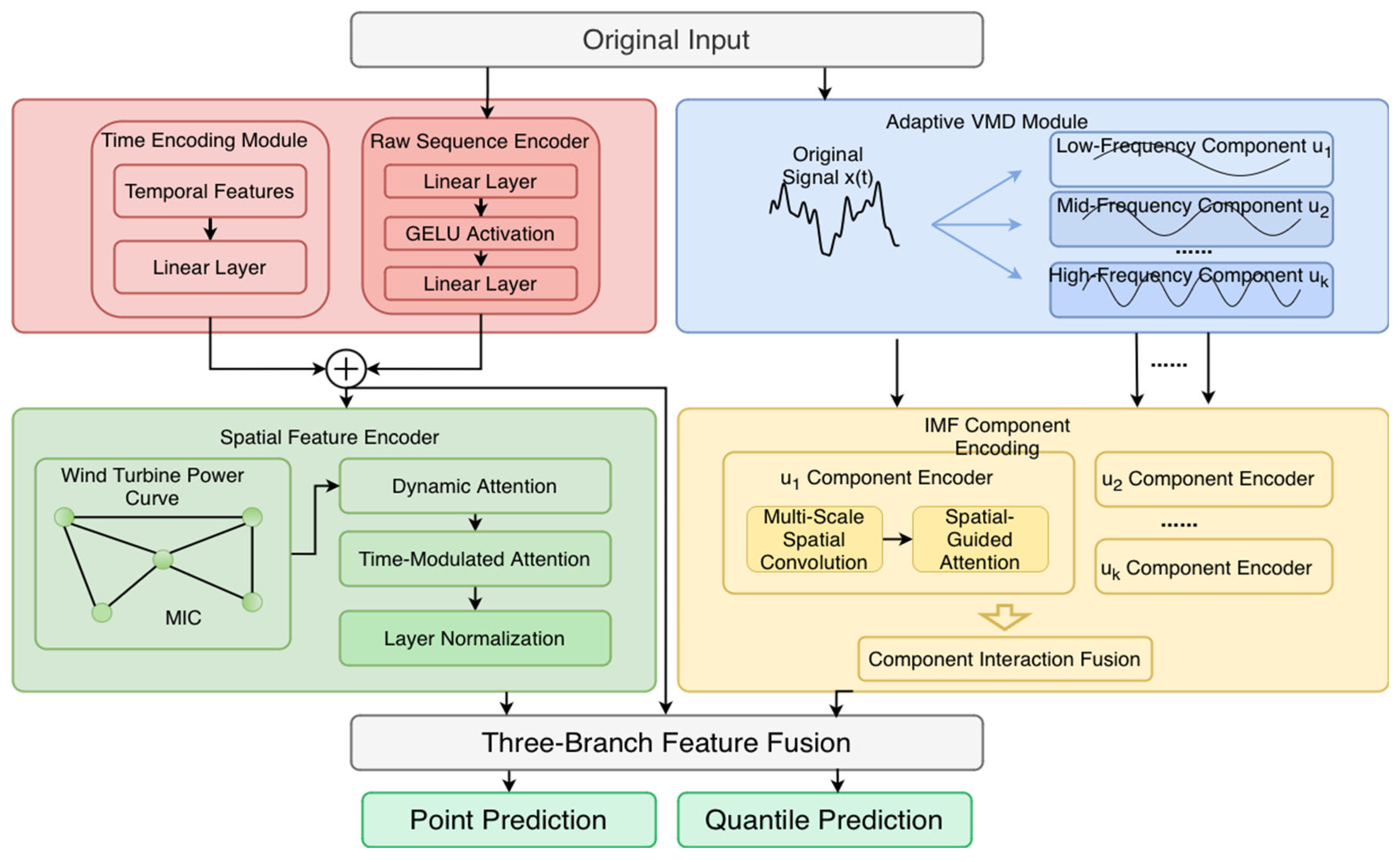
This paper presented VSTCformer, a unified framework for wind power interval forecasting based on adaptive variational mode decomposition, raw-sequence/global-context encoding, dynamic spatial feature encoding, component-wise temporal encoding, spatio-temporal cross-attention, inter-IMF interaction, three-way fusion, and multi-quantile regression. The model decomposes the raw power sequence into frequency-aligned intrinsic components, preserves the global temporal context of the undecomposed multivariate sequence, and integrates component-level temporal evolution with spatial dependency information through both implicit and explicit fusion mechanisms before estimating predictive quantiles. Compared with existing interval forecasting methods, the main advantage of VSTCformer lies in its unified design that combines adaptive signal decomposition, hierarchical spatio-temporal representation learning, and direct multi-quantile prediction within a single framework. Rather than optimizing these components independently, the proposed architecture jointly learns multiscale representations and predictive uncertainty, thereby achieving a better balance between point forecasting accuracy, interval sharpness, and calibration.

Experiments on SDWPF and GEFCom2012 demonstrate that VSTCformer maintains strong point-forecast accuracy while delivering clearly superior interval forecasts. In point forecasting, it achieves the lowest MSE at 6 h and 12 h on both datasets and remains essentially on par with GSTAformer at 24 h. In interval forecasting, it produces the narrowest prediction intervals across all evaluated horizons and obtains the best CWC in four of the six dataset-horizon settings. At the 24 h horizon, the model yields PICP/PINAW/CWC values of 0.890/0.324/0.681 on SDWPF and 0.913/0.410/0.410 on GEFCom2012. The ablation results further confirm the necessity of adaptive VMD, dynamic graph attention, SGTA, TMSA, and inter-IMF interaction. Overall, the results verify that decomposition-enhanced spatio-temporal uncertainty modeling is an effective route for wind power interval forecasting. The proposed framework is applicable to wind power datasets with different degrees of stationarity, demonstrating robust performance on both highly nonstationary and relatively smooth operating conditions.

Future work may extend the present framework to wider operating scenarios, investigate more efficient decomposition strategies, and perform broader quantitative probabilistic benchmarking across additional datasets.