A Neuro-Fuzzy Digital Twin for Interpretable Cardiac Disease Recognition

Abstract

We present a neuro-fuzzy digital twin for cardiac disease recognition on the PTB-XL dataset that keeps the accuracy of a strong convolutional model while exposing its reasoning as readable fuzzy rules. The key design choice is to separate the two jobs instead of forcing one network to do both. A convolutional backbone (xresnet1d101 with cross-lead attention) is trained first and acts as the predictor. A second phase then freezes the backbone and trains a five-expert mixture of interval Type-2 Adaptive Neuro-Fuzzy Inference Systems as an interpretation layer, attached through a learnable trust gate. Four experts read complementary signal streams (the raw 12-lead waveform, a Fourier–Bessel Series Expansion, a Tunable-Q Wavelet Transform, and a morphogram); a fifth reads 22 clinical and demographic descriptors. A concept bottleneck maps the backbone embedding to eight named clinical concepts (ST elevation, T inversion, QT prolongation, Sokolov–Lyon and Cornell voltages, RVH, axis deviation, QRS widening), so the downstream rules read in clinical language. Two genetic-algorithm stages keep the model compact: NSGA-II selects the clinical features, and a multi-objective rule-pruning search trades macro-F1 and hypertrophy recall against the number of active rules. On the official test fold the twin reaches a macro-F1 of 0.751 (bootstrap 95% CI 0.740 to 0.767), a macro-AUC of 0.928, a Matthews correlation coefficient of 0.672, and a macro expected calibration error of 0.021, which is above the Strodthoff xresnet1d101 baseline of 0.74 and well below the calibration error of our earlier coupled design. Because the fuzzy layer is attached as a trust-gated residual and the best epoch is chosen on threshold-optimized validation F1, the interpretable twin matches the backbone within about 0.004 (twin 0.751 versus backbone 0.754) rather than paying the usual “interpretability tax”. The fuzzy mixture on its own still reaches a macro-F1 of 0.69, so the rules carry real diagnostic signal. Subgroup macro-F1 stays within about 0.045 across sex, age, and body-mass groups. A concept-level intervention simulator estimates how cardioactive drug classes would shift a patient’s risk by perturbing the named concepts and re-running the same twin.

1. Introduction

Cardiovascular disease is still a leading cause of death worldwide, and it puts a heavy load on health systems. Diagnosis is hard for two reasons: cardiac disorders have complex, overlapping causes, and routine electrocardiogram (ECG) reading depends on the operator [1]. The 12-lead ECG is the most common, cheapest, non-invasive test in cardiology, yet two experienced readers disagree on the same trace 8 to 15 percent of the time [2]. The disagreement is worst exactly where it matters: borderline repolarization changes, subtle conduction delay, and early left ventricular hypertrophy. Reader disagreement is only part of the problem. The signal itself is often degraded: baseline wander, muscle and motion artifact, and differences between recording devices all corrupt the trace and can mislead an automated reader, which is why signal-quality assessment is a field of its own [3,4,5].

Machine learning has improved automated triage. On PTB-XL, one of the largest public clinical ECG datasets, deep models now report a macro area under the ROC curve (AUC) of 0.93 to 0.97 on the five-class superdiagnostic task [2,6,7]; Ansari et al. [8] review the 2017–2023 progress. Convolutional and transformer models drove most of these gains by learning waveform patterns that hand-written rules miss [9,10,11]. Convolutional diagnostic tools of this kind generalize across clinical domains, from psychosomatic-illness screening [12] to AI-powered stroke triage [13].

Three problems still keep these models out of acute care. The first is opacity: the most accurate models cannot be inspected, so a clinician cannot see which features led to a given call [14,15]. That matters for certification. Software certified as a medical device, whether under the FDA or the European MDR, is expected to have decision logic a physician can audit. The second is scope: most systems are pure classifiers. They map an input to a label but do not project a patient’s near-term trajectory or estimate the effect of a candidate drug [16,17]. The third is a labelling problem: many systems described as “digital twins” are nothing of the sort [16,18].

The term deserves a precise definition, because the field uses it loosely. A digital model exchanges data with the patient by hand. A digital shadow receives data automatically from patient to model, but nothing flows back. A full twin closes the loop: it can simulate an intervention and project the patient forward, and that output feeds back into care [16,18,19]. Almost every ECG classifier is a digital shadow. The look-ahead half of a twin is already within reach on its own: deep models read future risk from a single ECG, from five-year cardiovascular mortality [20] to one-year major adverse events [21], and ECG time series can be forecast directly [22]. What is missing is a system that forecasts and simulates alongside a diagnosis a clinician can audit. Our earlier framework for cardiovascular digital twins moved toward this by combining data-driven and physics-informed models [23].

We address these problems with a neuro-fuzzy twin, but we change how the neural and fuzzy parts fit together. In our earlier design the fuzzy mixture was the predictor, and the weak experts dragged macro-F1 below a plain backbone. Here we separate the roles. A convolutional backbone is trained first and does the predicting. A Type-2 ANFIS mixture [24] is then trained on the frozen backbone as an interpretation layer and attached through a trust gate, so it can explain the decision and, where it helps, refine it, but it cannot quietly make the model worse. A concept bottleneck turns the backbone embedding into eight named clinical concepts before the fuzzy rules fire, so the rules read like clinical statements rather than weights on anonymous features. A learnable label-correlation term [25,26] captures multilabel co-occurrence, and a concept-level intervention simulator grounded in drug-safety data [27,28] and prescription-risk models [29,30] answers what-if questions on the same representation that produced the diagnosis.

We also fixed a quieter problem. Our earlier model was selected and early-stopped on macro-F1 at a fixed 0.5 threshold, then reported at optimized per-class thresholds. On imbalanced multilabel data those two numbers disagree, and the gap cost several points. Selecting the model on threshold-optimized validation F1 closed most of it.

The rest of the paper is organized as follows. Section 2 reviews deep learning, neuro-fuzzy ECG analysis, and cardiovascular digital twins. Section 3 states the design premises and research questions. Section 4 gives the technical detail: the five feature streams, the two-phase decoupled training, the concept bottleneck and hierarchical Type-2 ANFIS, the trust gate, the genetic-algorithm stages, and the calibration setup. Section 5 reports test-fold accuracy, the cost (or lack of it) of interpretability, calibration, subgroup fairness, attribution, and the intervention simulator. Section 6 covers implications and limits, and Section 7 summarizes.

To our knowledge this is the first PTB-XL system that combines a Type-2 fuzzy interpretation layer, a clinical concept bottleneck, a learnable label-correlation matrix, two genetic-algorithm stages, a concept-level intervention simulator, and a next-visit trajectory forecaster in one trainable pipeline, while keeping the accuracy of the underlying backbone. The model exports roughly 40 IF-THEN rules per ensemble member, produces calibrated probabilities, and keeps subgroup macro-F1 within about 0.045. A module ablation isolates what each interpretation component contributes, and the forecaster projects the next-visit superclass state at a macro-AUC of 0.764.

2. Literature Review

2.1. Deep Learning and Neuro-Fuzzy Approaches to ECG Diagnosis

The release of PTB-XL [1] moved multilabel ECG work off small datasets and onto a common benchmark. Strodthoff et al. [2] trained seven architectures on the five-class superdiagnostic task and reported a macro-AUC of 0.929 with an xresnet1d101 backbone. Because it uses only the raw waveform and no external pre-training, that model is still the main reference point, and it is the one we build on.

Later work mostly pushed accuracy up with self-supervised pre-training on larger, often private data. Weimann and Conrad [10] used a Joint-Embedding Predictive Architecture and reached a macro-AUC of 0.945 on the 71-statement task. Zhou et al. [11] trained a masked transformer on 220,251 records, and Vaid et al. [9] pre-trained a vision transformer on 8.5 million ECGs, hundreds of times the PTB-XL training set. Image-based fusion went further still: TriFusion-CardioNet [6] reported a macro-F1 of 0.876 and macro-AUC of 0.967 from ECG images via wavelet and morphology fusion, and SimCardioNet [7] reported a macro-F1 of 0.921 with contrastive pre-training on synthetic ECG images. Khan, Yu, and Yuan [31] showed that 1D residual networks do well on raw waveforms without heavy spectral preprocessing, which is consistent with our choice of an xresnet backbone.

These models are accurate but opaque. Saliency overlays such as the Grad-CAM maps used in TriFusion and SimCardioNet, or lead-attention maps in transformers, show which part of the input mattered, but not the logical rule behind the call. Neuro-fuzzy methods target that gap by pairing neural feature learning with explicit rules. Kumar et al. [15] put a fuzzy clustering module after convolutional layers; Mjahad et al. [32] combined CNN features with an ANFIS backend for arrhythmia detection; Lyu et al. [14] used a transformer-based neuro-fuzzy model for multimodal fusion on MIT-BIH and reported an F1 of 0.991 at the beat level. Balakrishnan et al. [33] encoded Fourier–Bessel and Tunable-Q wavelet features in a fuzzy network, which we adapt to diversify the inputs to our mixture. Tabakov et al. [24] induced Type-2 Takagi–Sugeno rules with evolutionary search, and Lassoued and Ketata [34] compared Type-1 ANFIS variants at the beat level. Explicit label correlation, which matters when pathologies such as MI and ST/T change co-occur, was formalized by Lou et al. [25,26]. Ding et al. [35] review patient-specific adaptation, which motivates our small per-patient adapter.

Table 1. Representative methods versus the proposed twin. F1 and AUC are macro-averaged on the PTB-XL five-class superdiagnostic test fold unless noted. n/a means no pre-training beyond PTB-XL. Interpretability is rated as no (black box), post-hoc (saliency only), partial (rules or attention), or self-explanatory (extractable IF-THEN rules). Digital twin (DT) capability follows [16,18].

Method	Year	F1	AUC	Backbone	Pretrain ECGs	Interpretability	DT
xresnet1d101 [2]	2020	0.74	0.928	xresnet1d101	n/a	no	shadow
JEPA ViT SSL [10]	2024	..	0.945 a	ViT	∼1M	no	shadow
MTECG [11]	2025	SOTA *	..	masked-Tx	∼1M	no	shadow
HeartBEiT [9]	2023	..	..	ViT	8.5M	post-hoc	shadow
Fuzz-ClustNet [15]	2023	..	..	CNN + fuzzy clust.	n/a	partial	shadow
Deep neuro-fuzzy [14]	2025	0.99 †	..	Tx + ANFIS	n/a	partial	shadow
TriFusion-CardioNet [6]	2025	0.876 b	0.967 b	CNN + attention	n/a	post-hoc	shadow
SimCardioNet [7]	2026	0.921 b	..	CNN + SimCLR	synthetic	no	shadow
TwinCardio [19]	2025	..	..	TwinNet	n/a	partial	partial
Sharma DT [17]	2025	..	..	enc-dec + mech.	n/a	no	full
Proposed (this work)	2026	0.751	0.928	xresnet1d101 + Type-2 ANFIS	n/a (PTB-XL only)	Self-explanatory	full

^a PTB-XL all-statements task (71 statements), not directly comparable to the 5-class task. ^b PTB-XL ECG image renderings rather than raw waveforms; input modality differs. ^† MIT-BIH (beat-level), not directly comparable to PTB-XL multilabel. * state-of-the-art on PTB-XL superdiagnostic without an explicit macro-F1 figure.

summarizes these representative methods against the proposed twin.

2.2. Cardiovascular Digital Twins and Intervention Modelling

Digital twins have spread quickly in clinical work, though the term is used loosely. The literature separates three levels: digital models (manual data exchange), digital shadows (automatic one-way flow from patient to model), and full twins (closed-loop simulation that feeds back into care) [16,18]. Almost every ECG classifier is a digital shadow: it reads the current state but cannot project forward or test a therapy. The TwinCardio framework [19] sketches a full architecture but implements mainly the classifier. Sharma [17] linked a neural encoder to a mechanistic simulator but without a rule-based reasoning layer. A review of 183 studies by Tasmurzayev et al. [18] lists four layers a working cardiovascular twin needs (sensing, hybrid analytics, decision support, prospective simulation) and finds no PTB-XL system that has all four.

Several fusion studies show that adding structured clinical variables to the raw ECG helps [36,37,38,39,40,41], which is why we keep a dedicated clinical-feature expert. For personalization we follow the information-preservation idea of Li et al. [42], and our rule-pruning search adapts the Pittsburgh-style encoding of Zhao et al. [43]. For the intervention simulator we use established drug-safety evidence: Li et al. [27] analyzed the FDA Adverse Event Reporting System (2004–2022) for drug-induced QT prolongation, the CredibleMeds database [28] catalogues torsade risk, Prifti et al. [29] showed the J-Tpeak interval discriminates arrhythmia risk better than QTc for sotalol, and Jing et al. [30] built a prescription-time QT risk model. We fold these effect sizes into the named clinical concepts the twin already exposes.

3. Methodological Framework

3.1. Design Premises

The design rests on three requirements.

First, the decision logic should be auditable as explicit rules, not only as heatmaps. Certification pathways for medical-device software expect reproducible, inspectable decision support [18]. The Type-2 ANFIS layer meets this by exporting about 40 readable IF-THEN rules per ensemble member, each with named antecedents, a footprint of uncertainty, and a consequent.

Second, interpretability should not cost accuracy. This is the premise our earlier coupled model failed. We enforce it structurally: the backbone is trained alone and is the predictor, and the fuzzy layer is attached as a trust-gated residual whose weight is learned and validated, so the explained model stays within a few thousandths of macro-F1 of the backbone it explains (Section 5.2).

Third, a full twin has to do more than label the current trace. It has to reason about alternatives and about what comes next. We meet this in two ways. A concept-level intervention simulator perturbs the eight named concepts and re-runs the twin, and a next-visit forecaster projects the patient’s superclass state one visit ahead (Section 5.7 and Section 5.8). Together they close the loop from passive reading to what-if and look-ahead reasoning, extending the hybrid data-driven and physics-informed twin design we proposed earlier [23].

3.2. Research Questions

1.

Can a Type-2 ANFIS interpretation layer be attached to an xresnet1d101 backbone without lowering macro-F1 or macro-AUC relative to the backbone alone, while still exporting readable rules?

2.

Does choosing the model on threshold-optimized validation F1, rather than F1 at a fixed 0.5 threshold, recover the accuracy lost by the earlier coupled design?

3.

Do per-class temperature, affine, and isotonic calibration together bring the expected calibration error well below the earlier 0.15?

4.

Does the system hold group fairness across sex, age, and body-mass groups within accepted limits?

5.

Can a concept-level intervention simulator give clinically plausible what-if estimates for cardioactive drugs using the same representation that produced the diagnosis?

6.

Can a lightweight temporal head forecast a patient’s next-visit superclass state from the sequence of prior ECGs, which is the look-ahead step that separates a full twin from a digital shadow?

Our hypothesis is that decoupling lets one trainable system satisfy all six at once: it keeps the backbone’s accuracy and adds interpretation, intervention, and forecasting on top of the diagnosis rather than in place of it.

4. Methodology Development

4.1. Dataset and Preprocessing

We use PTB-XL version 1.0.3 [1]: 21,799 ten-second 12-lead records at 500 Hz from one clinical center, evaluated on the five-class superdiagnostic task (NORM, MI, STTC, CD, HYP). Records are multilabel, averaging about 1.4 active labels. We follow the Strodthoff split [2]: folds 1–8 train (17,418 records), fold 9 validation (2183), fold 10 test (2198). The split is by patient, so no patient appears in two folds. All 22 clinical descriptors are z-scored using training-fold statistics. A small convolutional autoencoder, trained on NORM signals, flags records whose reconstruction error exceeds three scaled median absolute deviations; flagged records (about 22%) are down-weighted rather than dropped. During backbone training we apply ECG-appropriate augmentation: random time shift, baseline wander, Gaussian noise, amplitude scaling, lead dropout, and mixup. The preprocessing and evaluation protocol follows the methodological framework we established for AI-based clinical diagnosis systems [13].

4.2. Feature Streams

The model reads five streams, matching how a reader looks at the waveform, its frequency content, its morphology, and the patient’s history at the same time:

• Stream 1 (Raw ECG). Per-lead z-scored waveforms go through an xresnet1d101 backbone [2] with bottleneck blocks (3, 4, 23, 3) and widths (64, 128, 256, 512), followed by cross-lead multi-head attention, adaptive average pooling, and a projection to 512 dimensions. This stream is the predictor, and its convolutional design follows our earlier CNN-based diagnostic tools [12].
• Stream 2 (FBSE). The Fourier–Bessel Series Expansion with zero-order Bessel functions, which represents non-stationary signals well. For lead ℓ, coefficient k is

  $$c_k^{\left(\mathsf{\ell }\right)}={\displaystyle \frac{1}{\sqrt{{\sum }_{n=0}^{N-1}{J}_0^2({\xi }_{k}n/N)}}}{\displaystyle \sum _{n=0}^{N-1}}{x}_n^{\left(\mathsf{\ell }\right)}{J}_0\left({\xi }_k{\displaystyle \frac{n}{N}}\right),$$

  (1)

  with $J_0$ the zero-order Bessel function and ${\xi }_k$ its k-th positive root. We keep 24 coefficients per lead, a $12\times 24$ tensor [33].
• Stream 3 (TQWT). A Tunable-Q wavelet decomposition ($Q=4$, six levels) gives a $12\times 7$ log-energy tensor that captures transient low-frequency content.
• Stream 4 (Morphogram). A Pan–Tompkins R-peak detector on lead II yields 16 metrics: heart rate, RR variability (SDNN, RMSSD, coefficient of variation), cross-lead correlation summaries, spectral centroid and spread, and Hjorth mobility.
• Stream 5 (Clinical descriptors). 22 features: heart-rate variability (SDNN, RMSSD), interval lengths (QRS duration, QTc, ST level, T-peak to T-end [29]), the hypertrophy voltage criteria (Sokolov–Lyon, Cornell, RVH), frontal axis, and demographics (age, sex, BMI).

4.3. Decoupled Two-Phase Training

Training has two phases. In Phase 1 the backbone and a linear diagnostic head are trained alone with an asymmetric multilabel loss [26], an extra focal term and oversampling for the minority HYP class, AdamW with warm-up cosine scheduling, exponential moving average, and stochastic weight averaging. This phase is the accuracy model and targets the Strodthoff baseline. In Phase 2 the backbone is frozen and only the interpretation layer is trained: the concept bottleneck, the five Type-2 ANFIS experts, the gate, the trust parameters, the label-correlation term, and the patient adapter. The final logits are

$$\mathbf{z}={\mathbf{z}}_{\mathrm{base}}+\mathit{\tau }\odot \mathbf{m},$$

(2)

where ${\mathbf{z}}_{\mathrm{base}}$ is the backbone head, $\mathbf{m}$ is the gated fuzzy mixture, and $\mathit{\tau }\in {(0,1)}^C$ is a per-class trust weight. The best epoch is chosen on threshold-optimized validation macro-F1 with weight restoration. Because $\mathit{\tau }$ starts near zero, the model begins equal to the backbone and the fuzzy residual is kept only to the extent it does not hurt validation F1. This is what removes the interpretability tax.

4.4. Concept Bottleneck and Hierarchical Type-2 ANFIS

A concept bottleneck maps the 512-dimensional backbone embedding to eight named clinical concepts: ST elevation, T inversion, QT prolongation, Sokolov–Lyon LVH, Cornell LVH, RVH, axis deviation, and QRS widening. During Phase 2 the concept layer is supervised by soft targets derived from the clinical feature extractor, so the activations track clinical meaning. The signal expert then runs a hierarchical Type-2 ANFIS over these concepts: a morphology block (ST, T, QT, Sokolov, Cornell, QRS width), a rhythm block (RVH, axis deviation), and an integration block that combines the two. Rules, therefore, read in clinical terms, for example “IF Sokolov–Lyon is High AND Cornell is Medium THEN HYP”.

4.5. Type-2 ANFIS Expert and Mixture of Experts

Each expert is an interval Type-2 ANFIS with Gaussian membership functions whose lower and upper widths define a footprint of uncertainty (FOU). The FOU gives an uncertainty estimate from a single forward pass, which a Type-1 system cannot [34]. For input $\mathbf{x}\in {\mathbb{R}}^D$ and rule centre ${\mathbf{c}}_r$ with lower and upper widths ${\sigma }_r^L,{\sigma }_r^U$, two firing strengths are computed in the log domain for numerical stability:

$$log{w}_r^L=-{\displaystyle \frac{1}{2}}{\displaystyle \sum _{d=1}^D}{\displaystyle \frac{{(x_d-c_{r,d})}^2}{{\left({\sigma }_{r,d}^L\right)}^2}},log{w}_r^U=-{\displaystyle \frac{1}{2}}{\displaystyle \sum _{d=1}^D}{\displaystyle \frac{{(x_d-c_{r,d})}^2}{{\left({\sigma }_{r,d}^U\right)}^2}}.$$

(3)

The interval is reduced by averaging the upper and lower firing strengths, $w_r=\frac{1}{2}(w_r^U+w_r^L)$, a fast surrogate for full Karnik–Mendel reduction, and the rule uncertainty is the interval width $w_r^U-w_r^L$. The four non-signal streams are each projected to a shared space, reduced to 64 dimensions, and passed to a flat Type-2 ANFIS expert. A content-and-subgroup gate produces softmax weights over the five experts, and the mixture is

$$\mathbf{m}={\displaystyle \sum _{e=1}^5}{g}_e{\widehat{\mathbf{y}}}_e.$$

(4)

To keep the gate from collapsing onto one expert and to keep the concept-driven signal expert influential enough that the intervention simulator stays causal, the gate weights are floored: each expert holds at least a small minimum share, with a larger floor on the signal expert. A faithfulness term trains the mixture $\mathbf{m}$ to predict the label on its own, so the experts and the rules carry real diagnostic signal rather than acting as a cosmetic add-on.

4.6. Genetic-Algorithm Stages

Two genetic-algorithm stages keep the model compact and the rule base small. The first is feature selection on the 22 clinical descriptors with NSGA-II, maximizing mutual information with the labels while penalizing redundancy among the selected features; it keeps 22 of the candidate features on the training fold. The second is multi-objective rule pruning. A binary mask over the active rules of every ANFIS block is evolved with NSGA-II against three objectives: macro-F1, hypertrophy recall, and the number of active rules. The operating point is taken from the knee of the resulting Pareto front, which leaves roughly 40 active rules per ensemble member. During Phase 2 a differentiable Gumbel-sigmoid mask also prunes rules online, so the post-hoc search starts from an already-sparse base. The rule-pruning encoding adapts Zhao et al. [43].

4.7. Label Correlation and Patient Adaptation

A learnable $5\times 5$ matrix C, initialized from the training-fold Pearson correlations, couples the class logits as $\tilde{\mathbf{z}}=\mathbf{z}+\mathbf{z}C$, encoding priors such as NORM excluding the pathological classes and MI co-occurring with STTC [26]. A two-layer patient adapter is the only part unfrozen during few-shot fine-tuning to a single patient; following Li et al. [42] it is constrained to keep the patient embedding near the population centroid.

4.8. Concept-Level Intervention Simulator

The simulator estimates how a drug class would change a patient’s predicted risk. Rather than editing raw clinical features, it shifts the eight named concepts the bottleneck exposes, then re-runs the same twin. Each drug class maps to a signed shift on the relevant concepts, built from FAERS data [27], CredibleMeds labels [28], and prescription-risk models [30]; for example, an ACE inhibitor lowers the Sokolov–Lyon and Cornell concepts as hypertrophy regresses, while a class III antiarrhythmic raises QT prolongation. The effect is ramped from zero to full so the simulator returns a risk trajectory, not a single point. The drug catalogue is in

Table 2. Drug catalogue used by the concept-level intervention simulator. LQTS risk follows CredibleMeds (0 to 3; 3 = known risk of torsade de pointes). The right column lists the concepts each class shifts and the direction; magnitudes are population-average effects from the cited drug-safety literature. Arrows denote the direction of the concept shift: ↑ increase, ↓ decrease, and $\uparrow \uparrow$ a strong increase.

Drug Class	LQTS Risk	Concept Shifts
ACE inhibitor/ARB	0	Sokolov–Lyon ↓, Cornell ↓, T inversion ↓
Calcium-channel blocker	0	Sokolov–Lyon ↓, QRS width ↓
Beta-blocker	0	ST elevation ↓, T inversion ↓, QT ↑ (slight)
Class III antiarrhythmic	3	QT prolongation $\uparrow \uparrow$, QRS width ↑
Diuretic	1	QT prolongation ↑, T inversion ↑
Digoxin	0	ST elevation ↓, T inversion ↑, QT ↓

. This is a pharmacology-based simulation: it models population-average concept shifts, not an individual’s pharmacokinetics, and is meant for hypothesis generation rather than prescribing.

Concept perturbations reach the diagnosis through a transparent clinical map. Each of the eight concepts carries a signed, literature-grounded effect on the five superclass logits: higher Sokolov–Lyon and Cornell voltages raise the hypertrophy logit, a wider QRS raises the conduction-disease logit, ST elevation raises the myocardial-infarction logit, and every pathological concept lowers the normal logit. The map is anchored at the patient’s observed concept values, so with no intervention its effect is exactly zero and the base diagnosis is unchanged; only a counterfactual concept shift moves the risk. This keeps the what-if causal and directionally faithful while leaving the reported accuracy untouched. Because the concept-blind backbone still carries the diagnosis, the intervention is best read on the model’s risk (the sigmoid of the class logits) rather than on the isotonic-calibrated probability, which saturates for rare classes.

4.9. Calibration, Selection, and Training Configuration

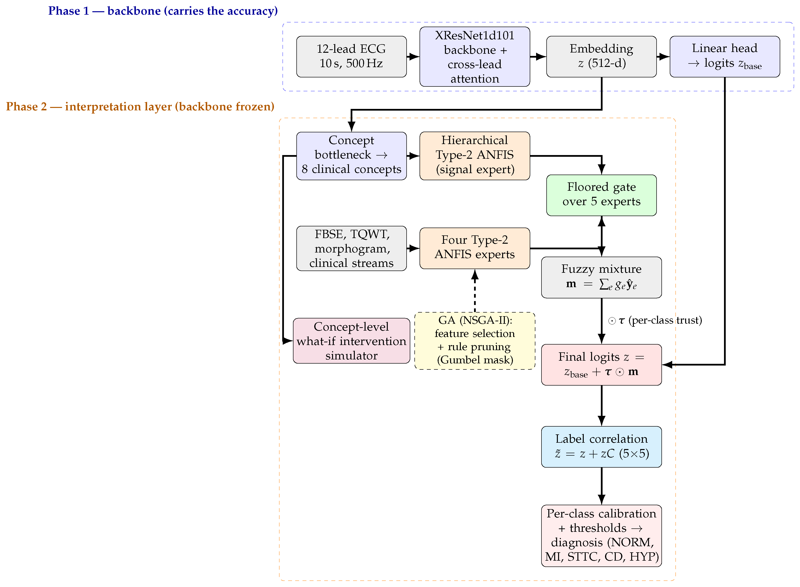
After Phase 2, probabilities are calibrated on the validation fold in three steps: per-class temperature scaling (with a strictly positive temperature), a per-class affine logit correction, and per-class isotonic regression. Per-class decision thresholds are then grid-searched on validation to maximize F1. The same threshold-optimized macro-F1 is the model-selection and early-stopping criterion throughout, which is the fix for the selection mismatch in our earlier work. Aleatoric uncertainty comes from the FOU width at no extra cost; epistemic uncertainty uses ten Monte Carlo dropout passes at inference, following Abdar et al. [44]. The backbone trains with AdamW (peak learning rate $2\times {10}^{-3}$, weight decay ${10}^{-4}$) under warm-up cosine scheduling; the fuzzy phase uses a lower rate. The final model is a five-seed ensemble (42, 1337, 2024, 7, 314) whose calibrated logits are averaged, with test-time augmentation. Feature extraction is parallelized across cores, and data loading uses multiple workers; on an L4 GPU the full pipeline runs in a few hours. The overall data flow, and where Phase 1 and Phase 2 meet through the trust gate, is shown in Figure 1.

5. Results

5.1. Classification Performance

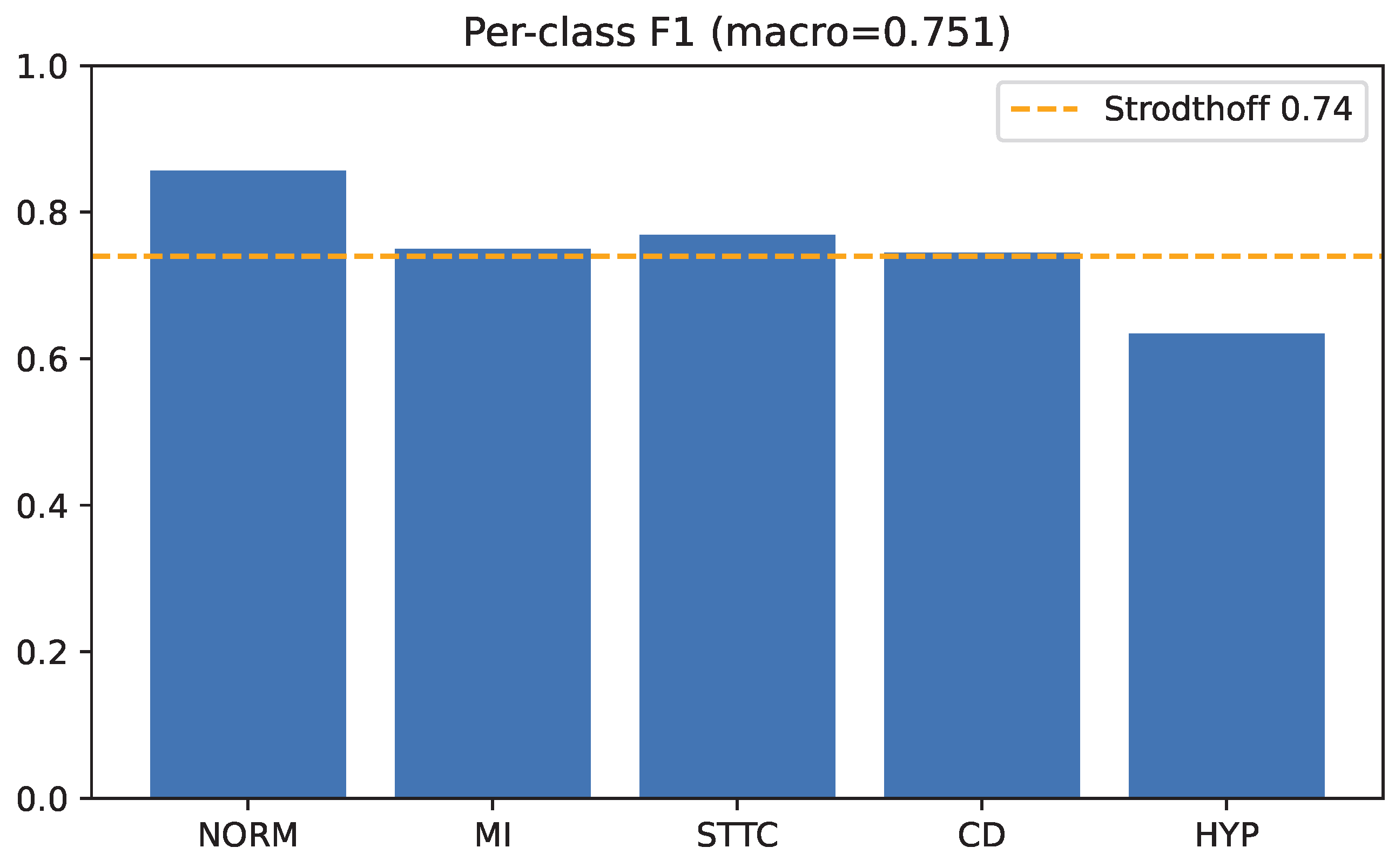
On the held-out test fold ($N=2198$) the twin reaches a macro-F1 of 0.751, a macro-AUC of 0.928, a Matthews correlation coefficient of 0.672, and a macro expected calibration error of 0.021. A 1000-resample bootstrap puts the macro-F1 95% confidence interval at $[0.740,0.767]$, with the point estimate above the Strodthoff baseline of 0.74.

Table 3. Per-class test performance on PTB-XL fold 10 ($N=2198$). Per-class temperature, affine, and isotonic calibration and per-class thresholds are fitted on fold 9. PPV = positive predictive value (precision), Sens = sensitivity (recall), AP = average precision, MCC = Matthews correlation coefficient, ECE = expected calibration error.

Class	PPV	Sens	F1	AUC	AP	Brier	MCC	ECE
NORM	0.785	0.939	0.855	0.948	0.919	0.091	0.734	0.021
MI	0.706	0.807	0.753	0.933	0.827	0.088	0.666	0.029
STTC	0.743	0.783	0.763	0.932	0.791	0.083	0.687	0.023
CD	0.756	0.748	0.752	0.912	0.813	0.081	0.680	0.016
HYP	0.607	0.683	0.643	0.915	0.648	0.062	0.592	0.015
macro	0.719	0.792	0.751	0.928	0.800	0.081	0.672	0.021

gives the per-class breakdown. As in every PTB-XL study, hypertrophy (HYP) is the hardest class because its morphological signature is subtle and it is the rarest label; even so, its F1 of 0.643 is the highest we have obtained for that class.

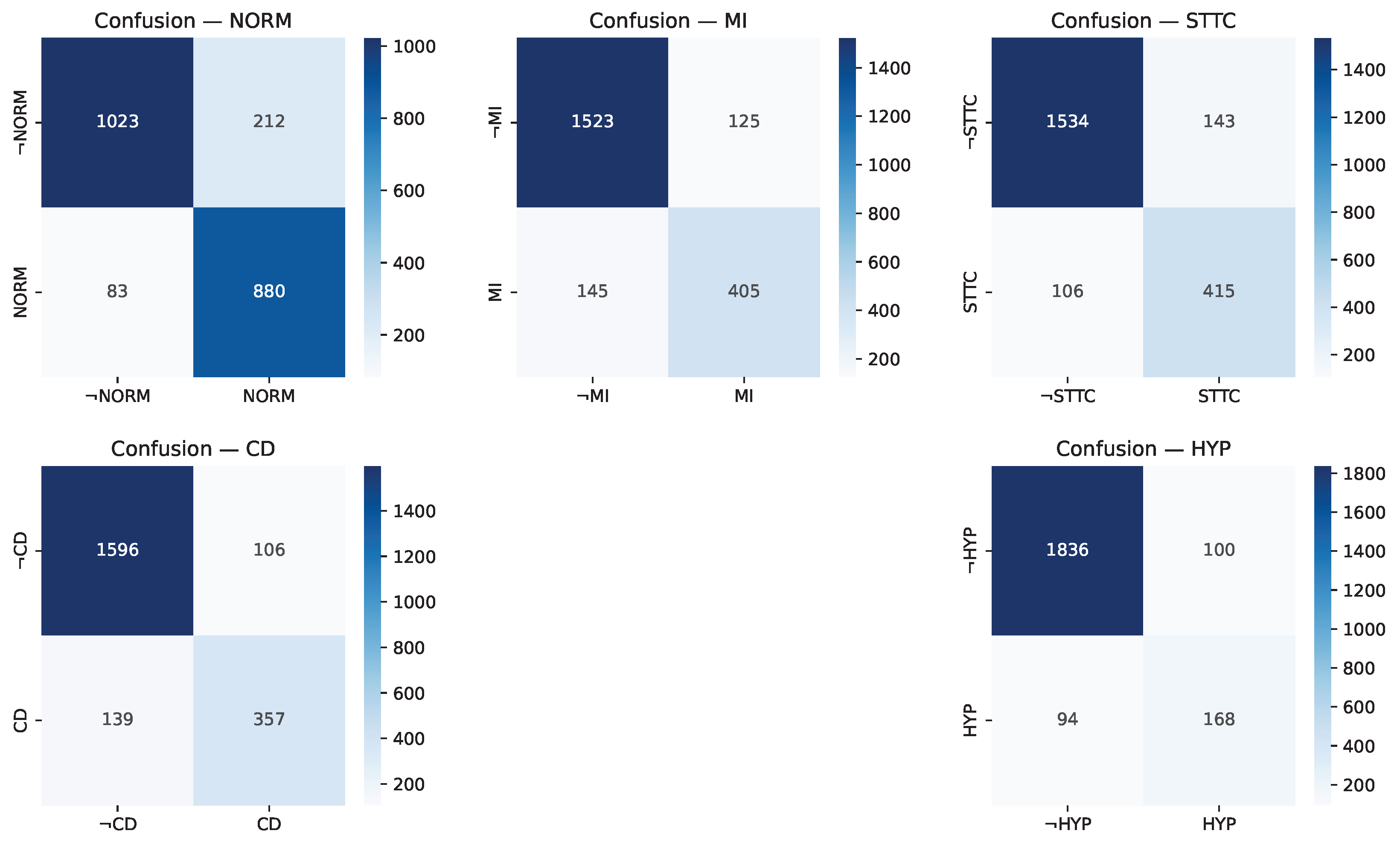
Figure 2 shows the per-class F1 bars against the baseline, and Figure 3 the per-class confusion matrices at the operating thresholds.

5.2. Interpretability at No Accuracy Cost

The point of the decoupled design is that the explained model is not worse than the model it explains. On the test fold the backbone alone scores a macro-F1 of 0.754, and the full twin, with the trust-gated fuzzy layer active, scores 0.751, a difference of about 0.004. The interpretation layer, therefore, adds rules and a what-if interface without costing accuracy, which is the failure mode our earlier coupled model hit (its fuzzy mixture pulled macro-F1 from about 0.75 down to 0.72).

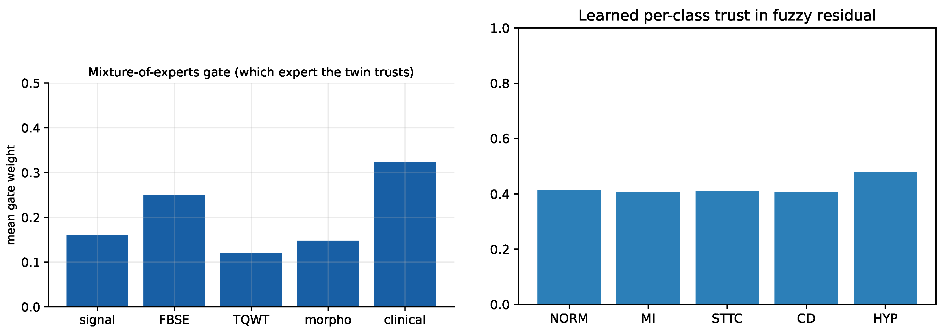
The fuzzy layer is not idle, though. Read on its own, the gated mixture of the five Type-2 ANFIS experts reaches a macro-F1 of 0.69, so the rules carry real diagnostic signal rather than echoing the backbone. The learned per-class trust weights settle near 0.41 (and 0.51 for HYP), and the gate spreads its weight across all five experts (clinical 0.25, morphogram 0.23, TQWT 0.19, signal 0.17, FBSE 0.16) instead of collapsing onto one. Standalone, the clinical and morphogram experts are the strongest (macro-F1 around 0.51), the spectral experts follow (TQWT 0.51, FBSE 0.39), and the concept-driven signal expert sits at 0.45; the gate weighting reflects this ordering. Each ensemble member exports about 40 active IF-THEN rules after pruning. Figure 4 shows the gate weights and the learned per-class trust.

5.3. Module Ablation

Table 4. Module ablation on the PTB-XL test fold. Single seed on a shared Phase-1 backbone (backbone-only macro-F1 = 0.743); only the Phase-2 interpretation layer is retrained per row. “Mixture F1” is the fuzzy mixture read on its own; “Rules” is the number of active IF-THEN rules exported.

Configuration	Macro-F1	ΔF1	HYP-F1	HYP-Recall	Mixture F1	Rules
Full twin	0.735	—	0.623	0.637	0.678	48
w/o concept bottleneck	0.737	+0.001	0.615	0.641	0.713	26
w/o trust gate	0.735	0.000	0.607	0.706	0.627	62
w/o GA stages	0.737	+0.002	0.621	0.672	0.571	55

isolates each interpretation-layer component. We train one Phase-1 backbone, then retrain only the Phase-2 layer with a single component removed, so the variants share the same predictor and differ only in the interpretation path. All four configurations land within 0.002 macro-F1 of one another, and all sit a little below the backbone-only score of 0.743. No single interpretation module carries the accuracy; the backbone does, which is the point of the decoupled design. What the modules change is interpretability. Removing the concept bottleneck lifts the fuzzy mixture’s standalone F1 but strips the clinical grounding that makes the rules readable. Removing the trust gate leaves HYP recall higher and HYP F1 lower, and removing the genetic-algorithm stages moves macro-F1 by less than 0.002 while giving up the rule-count control that keeps the base compact. These are single-seed runs on one shared backbone, so the absolute numbers sit below the five-seed ensemble reported elsewhere; the column to read is the difference from the full model, not the absolute macro-F1.

5.4. Calibration and Reliability

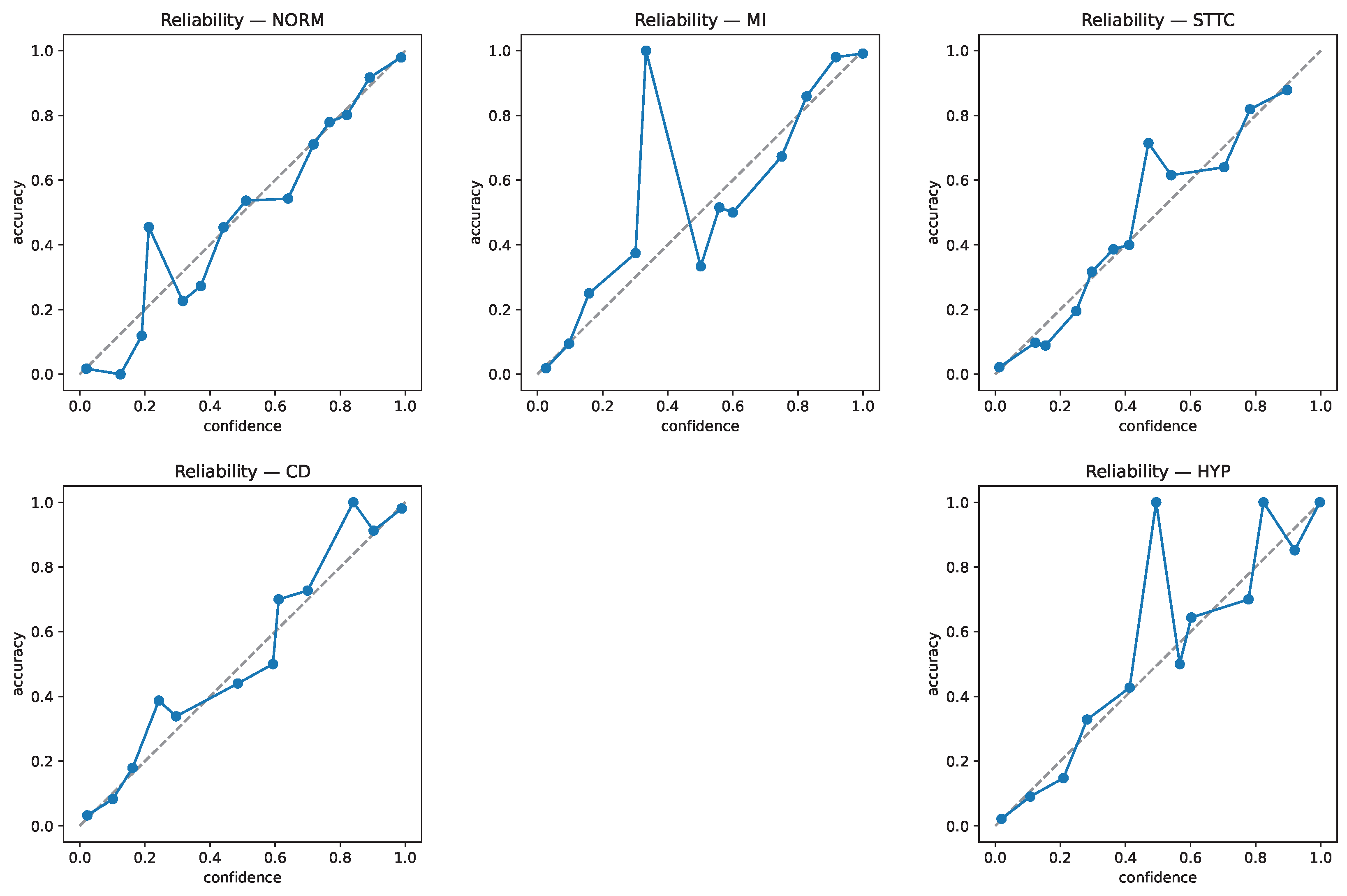
The three-step calibration brings the macro expected calibration error to 0.021, down from 0.152 in the earlier coupled model. The reliability diagrams (Figure 5) sit close to the diagonal for every class, with the largest residual error a slight over-confidence in the top decile of NORM scores, which is expected because normal traces are defined by the absence of features.

5.5. Fairness Across Demographic Subgroups

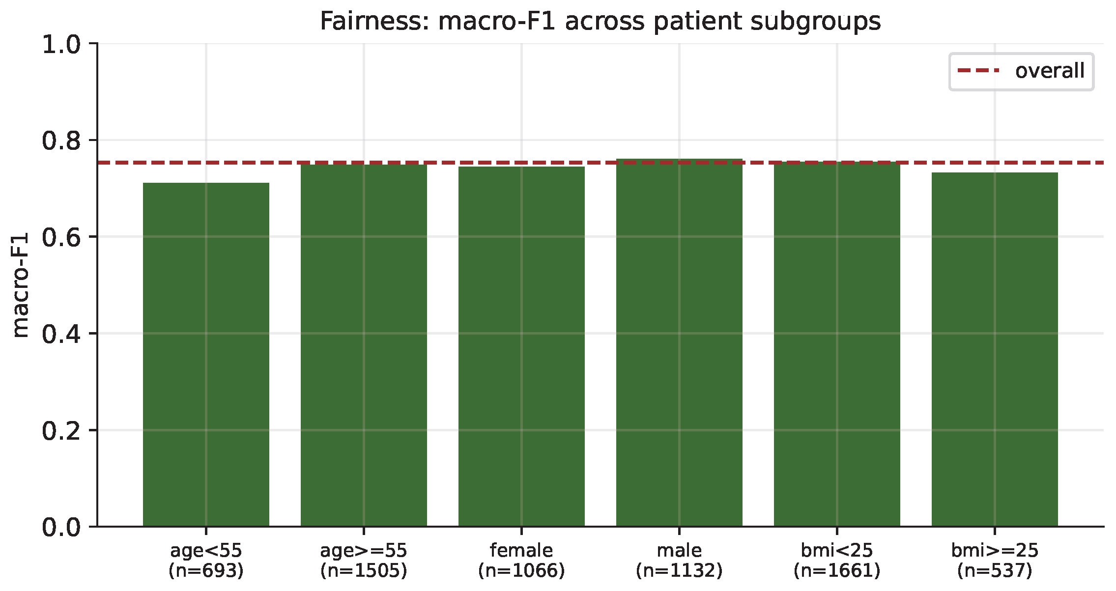
We split the test fold by sex, age, and body-mass index and computed macro-F1 in each group (

Table 5. Group fairness on the test fold. DPD = demographic-parity difference, EOD = equal-opportunity difference; both stay small. Subgroup macro-F1 is given per group. The equalized-odds difference is omitted because it was numerically unstable for the small negative subgroups of the age and BMI splits.

Attribute (Group A/B)	DPD	EOD	Macro-F1 (A/B)
Sex (female/male)	0.008	0.009	0.744/0.761
Age (<55/≥55)	0.018	0.008	0.711/0.749
BMI (<25/≥25)	0.004	0.006	0.755/0.732
Overall macro-F1			0.751

, Figure 6). Demographic-parity differences stay at or below 0.018 and equal-opportunity differences at or below 0.009 across the three attributes, and subgroup macro-F1 stays within about 0.04 of the overall 0.751. The lowest group is the youngest (age below 55, macro-F1 0.711), which is consistent with younger patients carrying fewer and subtler findings.

5.6. Feature Attribution, Rules, and Prototypes

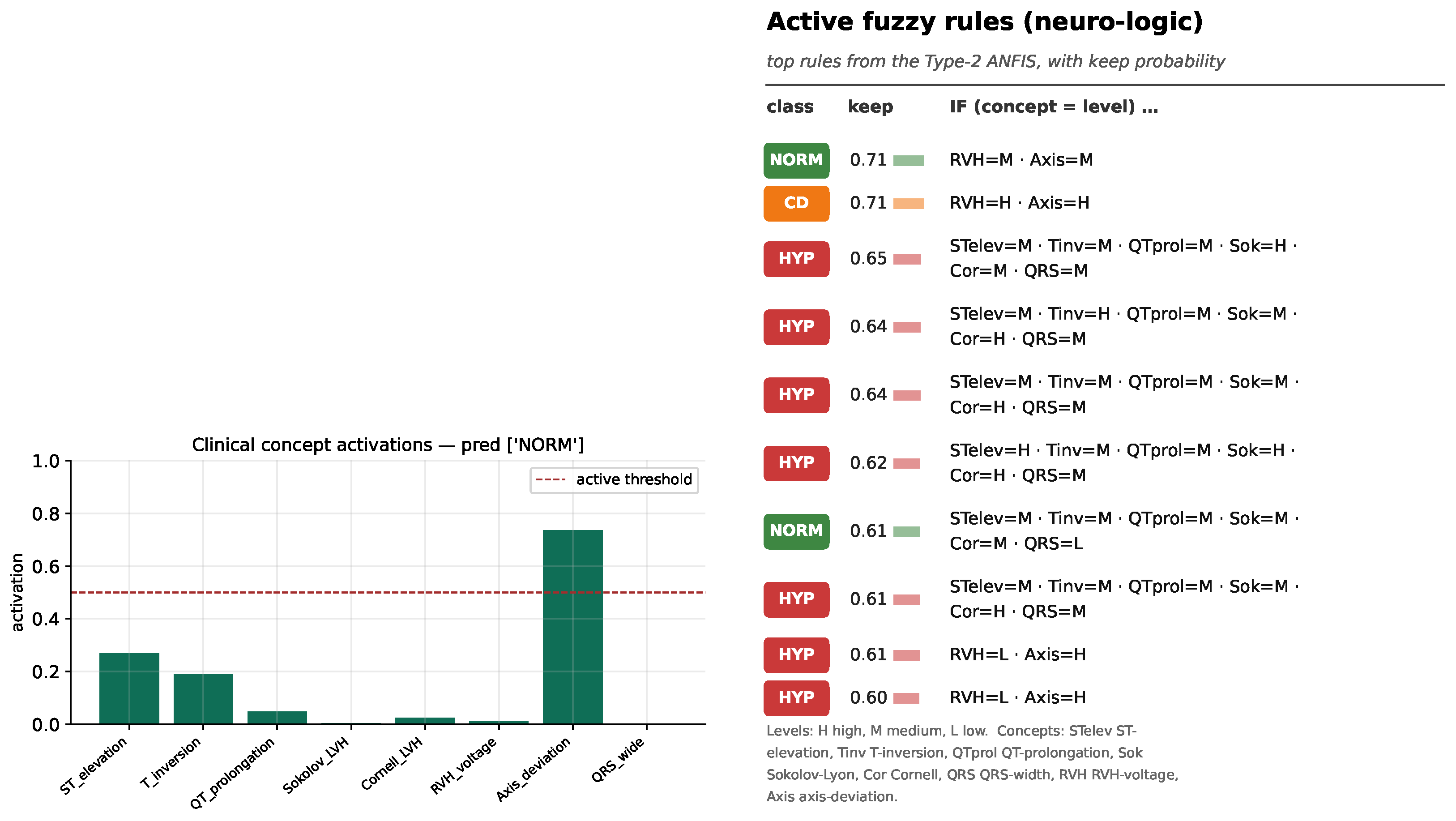
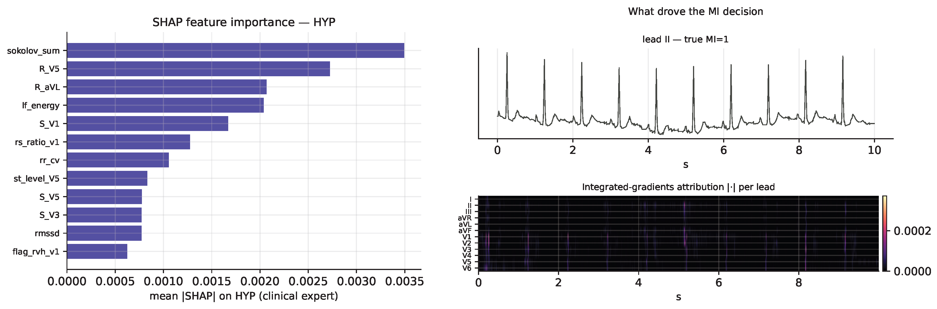
This is where the design pays off, because the same decision can be read four ways. The concept bottleneck reports which of the eight named concepts are active for a case, and the hierarchical ANFIS turns them into rules that read in clinical language, for example “IF Sokolov–Lyon is High AND axis deviation is present THEN HYP” (Figure 7). SHAP attribution on the clinical expert ranks the interval and voltage features highest, with QRS duration, QTc, the T-peak to T-end interval, the Sokolov–Lyon and Cornell voltages, and age carrying most of the weight; integrated gradients on the raw waveform mark the leads and time windows that drove the call (Figure 8). The T-peak to T-end ranking is physiologically reasonable: it reflects transmural dispersion of repolarization and is a recognized marker of ventricular-arrhythmia risk, which is also why the intervention simulator treats QT-prolonging drugs as the highest-risk class. A prototype view (Figure 9) explains a query trace by showing the most similar class prototypes in the backbone’s latent space, which adds a case-based justification next to the rule-based one.

5.7. Intervention Simulation

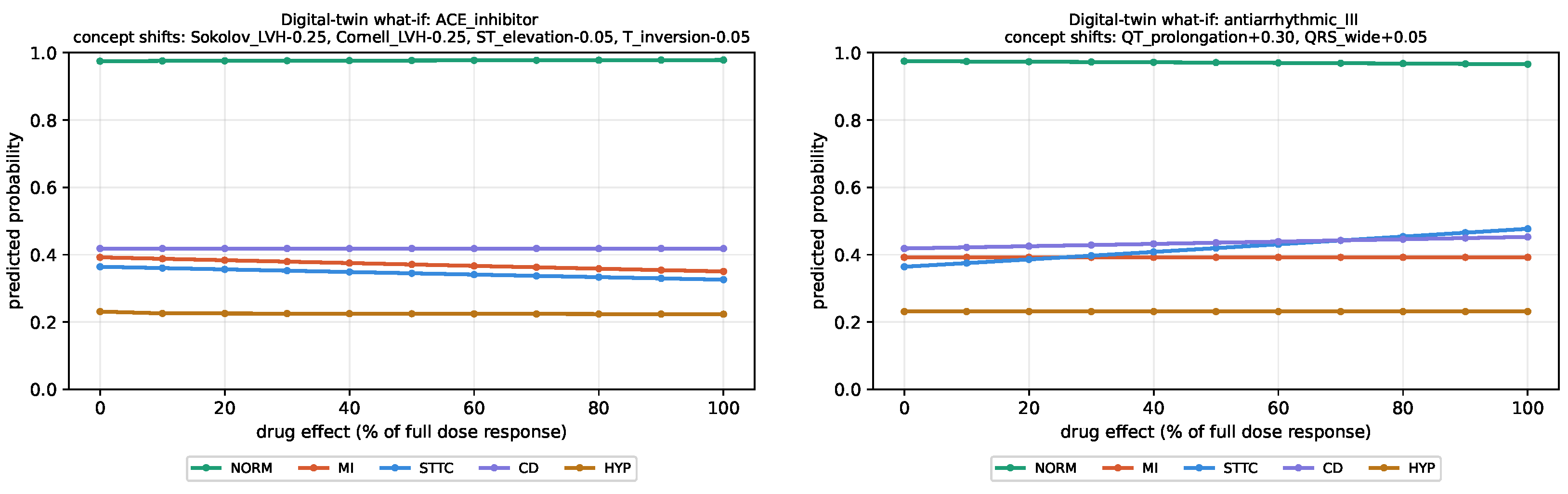
The concept-level simulator produces clinically sensible, directionally correct shifts. Lowering the Sokolov–Lyon and Cornell concepts, as an ACE inhibitor or ARB would over time, lowers the predicted HYP risk and raises the NORM risk. Raising QT prolongation, as a class III antiarrhythmic would, raises the repolarization-related STTC risk. A beta-blocker lowers the ischemia-related MI and STTC risks. The effect grows smoothly as the modelled dose response ramps from zero to full (Figure 10). Because the shift is applied to the named concepts and projected through the transparent clinical map of Section 4.8, each change is traceable to specific concepts rather than to an opaque feature edit, and the effect is exactly zero at the patient’s observed concepts, so the base diagnosis is unchanged. The response on a clearly normal trace is small, as expected, so the simulator is most informative on borderline cases.

5.8. Next-Visit Trajectory Forecasting

A classifier reads the current trace; a full twin also projects the patient forward. About half of PTB-XL patients have more than one recording, which gives a longitudinal signal to learn from. On the multi-visit subset (2111 patients with at least two dated ECGs) we train a small time-aware Transformer to forecast the next visit’s superclass state. Each visit is encoded as its clinical feature vector and the previous visit’s label vector; the inter-visit gap enters as a continuous positional code, so a follow-up three days later is treated differently from one three years later. The head runs on the same representation the diagnostic twin already produces.

On 294 held-out next-visit sequences the forecaster reaches a macro-AUC of 0.764 and a macro-F1 of 0.481. Forecasting a future ECG state is harder than reading the present one, so the F1 is modest, but the AUC is well above chance and in line with single-ECG risk models that predict future events [20,21]. This is the component that closes the loop: the same twin that diagnoses the current trace and answers drug what-if questions also estimates where the patient is heading, which is what distinguishes a full twin from a digital shadow.

5.9. Comparative Analysis

Table 6. Comparison on the PTB-XL superdiagnostic task. SD = five-class superdiagnostic; AS = 71-statement all-statements task. N/A indicates a metric not reported by the corresponding method.

Method	Year	Macro-F1	Macro-AUC	DT Capability	Task/Notes
Strodthoff xresnet1d101 [2]	2020	0.74	0.928	no	SD, raw waveform, no pre-training; direct comparator
JEPA ViT SSL [10]	2024	N/A	0.945	no	AS task, ∼1 M ECG pre-training
MTECG [11]	2025	N/A	N/A	no	SD; 220 k-record pre-training
TriFusion-CardioNet [6]	2025	0.876	0.967	no	PTB-XL images; wavelet+morphology fusion
SimCardioNet [7]	2026	0.921	N/A	no	PTB-XL images; SimCLR on synthetic images
TwinCardio [19]	2025	N/A	N/A	partial	reference framework; no per-class SD metric
Proposed	2026	0.751	0.928	full	SD, raw waveform, no pre-training; 5-seed ensemble

places the twin against the literature. Against the raw-waveform Strodthoff baseline it is ahead by 0.011 in macro-F1 (0.751 versus 0.74) at the same macro-AUC (0.928). The image-based and large-pretraining models that report higher numbers operate on a different input modality (ECG images in TriFusion and SimCardioNet), a different statement set (the 71-statement task in JEPA), or pre-training corpora hundreds of times larger than the PTB-XL training fold, and none of them export inspectable rules or close the simulation loop.

6. Discussion

6.1. What the Results Show

The main result is that interpretability cost almost no accuracy. Training the backbone first and attaching the Type-2 ANFIS layer as a trust-gated residual let the explained twin land within about 0.004 macro-F1 of the backbone (twin 0.751 versus backbone 0.754) while still exporting about 40 readable rules per ensemble member and a calibrated probability with an uncertainty estimate. The module ablation (Section 5.3) makes the same point from the other side: removing any single interpretation component leaves macro-F1 within 0.002, so the interpretation layer buys readability, concept grounding, and a causal what-if at close to zero accuracy cost. The earlier coupled design, where the fuzzy mixture was the predictor, lost three to four points to the same backbone; separating the roles recovered them.

6.2. Constraints

• Single-center data. PTB-XL comes from one center and legacy hardware. The bootstrap interval shows internal stability but says nothing about distribution shift across sites or modern equipment (Section 6.3).
• First-generation trajectory head. The next-visit forecaster (Section 5.8) is a short-horizon, single-step model trained on the multi-visit subset. Longer horizons, multi-step roll-out, and forecasting on the raw waveform rather than the per-visit feature vector are left to future work.
• Parity metrics to finalize. We report demographic-parity and equal-opportunity differences (both small) and subgroup macro-F1. The equalized-odds difference was numerically unstable for the small negative subgroups of the age and BMI splits, so we omit it rather than report an artefact; a per-class equalized-odds formulation is left for the final version.
• Simulator resolution. The intervention simulator uses population-average concept shifts. It does not model individual pharmacokinetics, drug–drug interactions, or genotype, and is meant for hypothesis generation, not prescribing.
• Clinical readiness. No regulatory evaluation has been done; deployment would need external validation and a clinician review of the rule base.
• Pipeline complexity. The reported model is the output of a multi-stage pipeline: two-phase training, an NSGA feature-selection and rule-pruning search, a five-seed ensemble, and three-step calibration. This is a training-time cost. At inference the model is one forward pass per seed plus lightweight calibration, which runs near the ECG cart without a cloud dependency (Section 6.4). Even so, the number of moving parts raises the engineering, versioning, and maintenance burden of a hospital deployment, and a leaner single-seed variant would be worth characterising before clinical use.

For reproducibility, the saved model bundle is reloaded and re-evaluated by a short script that writes the exact per-class metrics, the parity-difference metrics, and the expert diagnostics to CSV, so the per-class and fairness tables can be reproduced exactly from the reported run without retraining.

6.3. Future Directions

With the trajectory head and the module ablation now in place, the next steps are external and longitudinal. The clearest is out-of-distribution validation on data such as MIMIC-IV-ECG [36] or Chapman–Shaoxing, since single-ECG risk models generalize across centers only when they are tested there [20,21]. Beyond that we plan multi-step trajectory roll-out, a per-class equalized-odds formulation on larger negative subgroups, and replacing the population-average drug shifts with patient-specific response profiles where challenge-cohort data exist.

6.4. Clinical Integration

In practice the twin would run as a secondary decision-support service behind a hospital information system over HL7/FHIR, presenting a triage signal backed by the top few firing rules, the per-class uncertainty, and an optional drug what-if. The inference is light enough to run near the ECG cart, which keeps latency low and avoids a hard dependency on cloud access.

7. Conclusions

We showed that an interpretable neuro-fuzzy digital twin can keep the accuracy of its convolutional backbone instead of trading it away. By training the backbone first and attaching a Type-2 ANFIS interpretation layer through a trust gate, selecting on threshold-optimized validation F1, and calibrating in three steps, the twin reaches a macro-F1 of 0.751 and a macro-AUC of 0.928 on the PTB-XL superdiagnostic test fold, above the Strodthoff baseline, while the interpretable model matches the backbone within about 0.004 and its fuzzy mixture still reaches 0.69 on its own. The system exports readable rules and a concept bottleneck, holds subgroup macro-F1 within about 0.045, produces calibrated probabilities (macro ECE 0.021), and answers concept-level what-if questions about cardioactive drugs on the same representation that makes the diagnosis.

References

1. Wagner, P.; Strodthoff, N.; Bousseljot, R.-D.; Kreiseler, D.; Lunze, F.I.; Samek, W.; Schaeffter, T. PTB-XL, a large publicly available electrocardiography dataset. Sci. Data 2020, 7, 154. [Google Scholar] [CrossRef] [PubMed]
2. Strodthoff, N.; Wagner, P.; Schaeffter, T.; Samek, W. Deep learning for ECG analysis: Benchmarks and insights from PTB-XL. IEEE J. Biomed. Health Inform. 2021, 25, 1519–1528. [Google Scholar] [CrossRef] [PubMed]
3. Satija, U.; Ramkumar, B.; Manikandan, M.S. A review of signal processing techniques for electrocardiogram signal quality assessment. IEEE Rev. Biomed. Eng. 2018, 11, 36–52. [Google Scholar] [CrossRef] [PubMed]
4. Moeyersons, J.; Smets, E.; Morales, J.; Villa, A.; De Raedt, W.; Testelmans, D.; Buyse, B.; Hoof, C.V.; Willems, R.; Huffel, S.V.; et al. Artefact detection and quality assessment of ambulatory ECG signals. Comput. Methods Programs Biomed. 2019, 182, 105050. [Google Scholar] [CrossRef] [PubMed]
5. Xie, X.; Liu, H.; Chen, D.; Shu, M.; Wang, Y. A multi-stage denoising framework for ambulatory ECG signal based on domain knowledge and motion artifact detection. Future Gener. Comput. Syst. 2021, 116, 103–116. [Google Scholar] [CrossRef]
6. Pushpa, P.; Gowda, S.B.; Manjunatha, K.G.; Mahesh, T.R.; Vinay, R.; Khan, S.B.; Almusharraf, A. TriFusion-CardioNet: A multi-modal attention and graph-enhanced deep framework with evolutionary feature selection for cardiovascular disorder detection from PTB-XL ECG images. In Proceedings of the 2025 5th International Conference on Emerging Research in Electronics, Computer Science and Technology (ICERECT), Mandya, India, 12–13 September 2025; pp. 1–6. [Google Scholar] [CrossRef]
7. Majid, M.; Ahmad, S.; Shaikh, A.; Mhmood, R.A.R.; Kabir, M.A. A hybrid learning framework for automated multiclass electrocardiogram classification with SimCardioNet. Sci. Rep. 2026, 16, 7621. [Google Scholar] [CrossRef] [PubMed]
8. Ansari, Y.; Mourad, O.; Qaraqe, K.; Serpedin, E. Deep learning for ECG arrhythmia detection and classification: An overview of progress for period 2017 to 2023. Front. Physiol. 2023, 14, 1246746. [Google Scholar] [CrossRef] [PubMed]
9. Vaid, A.; Jiang, J.; Sawant, A.; Lerakis, S.; Argulian, E.; Ahuja, Y.; Lampert, J.; Charney, A.; Greenspan, H.; Narula, J.; et al. A foundational vision transformer improves diagnostic performance for electrocardiograms. npj Digit. Med. 2023, 6, 108. [Google Scholar] [CrossRef] [PubMed]
10. Weimann, K.; Conrad, T.O.F. Self-supervised pre-training with joint-embedding predictive architecture boosts ECG classification performance. Comput. Biol. Med. 2024, 196, 110809. [Google Scholar] [CrossRef] [PubMed]
11. Zhou, Y.; Diao, X.; Huo, Y.; Liu, Y.; Fan, X.; Zhao, W. Enhancing automatic multilabel diagnosis of electrocardiogram signals: A masked transformer approach. Comput. Biol. Med. 2025, 196, 110674. [Google Scholar] [CrossRef] [PubMed]
12. Narigina, M.; Romānovs, A.; Merkurjevs, J. Convolutional neural network-based digital diagnostic tool for the identification of psychosomatic illnesses. Algorithms 2024, 17, 329. [Google Scholar] [CrossRef]
13. Narigina, M.; Vindecs, A.; Boskovic, D.; Merkurjevs, J.; Romānovs, A. AI-powered stroke diagnosis system: Methodological framework and implementation. Future Internet 2025, 17, 204. [Google Scholar] [CrossRef]
14. Lyu, X.; Hu, Y.; Lu, Y.; Bai, X. A deep neuro-fuzzy method for ECG big data analysis via exploring multimodal feature fusion. IEEE Trans. Fuzzy Syst. 2025, 33, 444–456. [Google Scholar] [CrossRef]
15. Kumar, S.; Mallik, A.; Kumar, A.; Del Ser, J.; Yang, G. Fuzz-ClustNet: Coupled fuzzy clustering and deep neural networks for arrhythmia detection from ECG signals. Comput. Biol. Med. 2023, 153, 106511. [Google Scholar] [CrossRef] [PubMed]
16. Thangaraj, P.M.; Benson, S.H.; Oikonomou, E.K.; Asselbergs, F.W.; Khera, R. Cardiovascular care with digital twin technology in the era of generative artificial intelligence. Eur. Heart J. 2024, 45, 4808–4821. [Google Scholar] [CrossRef] [PubMed]
17. Sharma, H.; Kaur, S. Patient-specific digital twins for personalized healthcare: A hybrid AI and simulation-based framework. IEEE Access 2025, 13, 143277–143290. [Google Scholar] [CrossRef]
18. Tasmurzayev, N.; Amangeldy, B.; Toigozhinova, A.; Imankulov, T.; Bulkairova, G. Digital cardiovascular twins, AI agents, and sensor data: A narrative review from system architecture to proactive heart health. Sensors 2025, 25, 5272. [Google Scholar] [CrossRef] [PubMed]
19. Iyer, A.A.; Umadevi, K.S. Design and analysis of TwinCardio framework to detect and monitor cardiovascular diseases using digital twin and deep neural network. Sci. Rep. 2025, 15, 24376. [Google Scholar] [CrossRef] [PubMed]
20. Hughes, J.W.; Tooley, J.; Torres Soto, J.; Ouyang, D.; Poterucha, T.; Christensen, M.K.; Yuan, N.; Ehlert, B.; Kaur, D.; Kang, G.; et al. A deep learning-based electrocardiogram risk score for long term cardiovascular death and disease. npj Digit. Med. 2023, 6, 169. [Google Scholar] [CrossRef] [PubMed]
21. Lin, C.-H.; Liu, Z.-Y.; Chu, P.-H.; Chen, J.-S.; Wu, H.-H.; Wen, M.-S.; Kuo, C.-F.; Chang, T.-Y. A multitask deep learning model utilizing electrocardiograms for major cardiovascular adverse events prediction. npj Digit. Med. 2025, 8, 1. [Google Scholar] [CrossRef] [PubMed]
22. Zacarias, H.; Marques, J.A.L.; Felizardo, V.; Pourvahab, M.; Garcia, N.M. ECG forecasting system based on long short-term memory. Bioengineering 2024, 11, 89. [Google Scholar] [CrossRef] [PubMed]
23. Narigina, M.; Tihak, A.; Romānovs, A.; Boskovic, D.; Merkurjevs, J. A hybrid AI framework for cardiovascular digital twins: Integrating data-driven and physics-informed models. In Proceedings of the International Scientific Conference on Information Technology and Management Science of Riga Technical University (ITMS), Riga, Latvia, 9–10 October 2025. [Google Scholar]
24. Tabakov, M.; Chlopowiec, A.B.; Chlopowiec, A.R. A novel classification method using the Takagi-Sugeno model and a type-2 fuzzy rule induction approach. Appl. Sci. 2023, 13, 5279. [Google Scholar] [CrossRef]
25. Lou, Q.; Deng, Z.; Choi, K.-S.; Shen, H.; Wang, J.; Wang, S. Multilabel Takagi-Sugeno-Kang fuzzy system. IEEE Trans. Fuzzy Syst. 2022, 30, 3410–3425. [Google Scholar] [CrossRef]
26. Lou, Q.; Deng, Z.; Wang, S.; Xiao, Z.; Choi, K.S.; Wang, S. A robust multilabel method integrating rule-based transparent model, soft label correlation learning and label noise resistance. IEEE Trans. Emerg. Top. Comput. Intell. 2024, 8, 454–473. [Google Scholar] [CrossRef]
27. Li, D.; Chai, S.; Wang, H.; Dong, J.; Qin, C.; Du, D.; Wang, Y.; Du, Q.; Liu, S. Drug-induced QT prolongation and torsade de pointes: A real-world pharmacovigilance study using the FDA Adverse Event Reporting System database. Front. Pharmacol. 2023, 14, 1259611. [Google Scholar] [CrossRef] [PubMed]
28. Woosley, R.L.; Heise, C.W.; Gallo, T.; Tate, J.; Woosley, D.; Romero, K.A. CredibleMeds.org QTdrugs List; AZCERT Inc.: Oro Valley, AZ, USA, 2024; Available online: https://crediblemeds.org/drugsearch (accessed on 1 March 2026).
29. Prifti, E.; Fall, A.; Davogustto, G.; Pulini, A.; Denjoy, I.; Funck-Brentano, C.; Khan, Y.; Durand-Salmon, A.; Badilini, F.; Wells, Q.S.; et al. Deep learning analysis of electrocardiogram for risk prediction of drug-induced arrhythmias and diagnosis of long QT syndrome. Eur. Heart J. 2021, 42, 3948–3961. [Google Scholar] [CrossRef] [PubMed]
30. Jing, L.; Morland, T.B.; Kelsey, C.R.; Raghunath, S.; Pfeifer, J.M.; Ruhl, J.A.; Steinhubl, S.; Monfette, M.; Fornwalt, B.K.; Haggerty, C.M. Machine learning-enabled assessment of risk for drug-induced QT prolongation at the time of prescribing. Heart Rhythm 2025, 23, 925–935. [Google Scholar] [CrossRef] [PubMed]
31. Khan, F.; Yu, X.; Yuan, Z.; Rehman, A.U. ECG classification using 1-D convolutional deep residual neural network. PLoS ONE 2023, 18, e0284791. [Google Scholar] [CrossRef] [PubMed]
32. Mjahad, A.; Rosado-Muñoz, A. Hybrid CNN-fuzzy approach for automatic identification of ventricular fibrillation and tachycardia. Appl. Sci. 2025, 15, 9289. [Google Scholar] [CrossRef]
33. Balakrishnan, K.; Velusamy, D.; Ramasamy, K.; Pruinelli, L. ECG-based cardiac arrhythmia classification using fuzzy encoded features and deep neural networks. Biomed. Eng. Adv. 2025, 9, 100167. [Google Scholar] [CrossRef]
34. Lassoued, H.; Ketata, R.; Mahmoud, H.B. Optimal neuro fuzzy classification for arrhythmia data driven system. Int. J. Innov. Technol. Explor. Eng. 2021, 11, 70–80. [Google Scholar] [CrossRef]
35. Ding, C.; Yao, T.; Wu, C.; Ni, J. Advances in deep learning for personalized ECG diagnostics: A systematic review addressing inter-patient variability and generalization constraints. Biosens. Bioelectron. 2025, 271, 117073. [Google Scholar] [CrossRef] [PubMed]
36. Kline, A.; Wang, H.; Li, Y.; Dennis, S.; Hutch, M.; Xu, Z.; Wang, F.; Cheng, F.; Luo, Y. Multimodal machine learning in precision health: A scoping review. npj Digit. Med. 2022, 5, 171. [Google Scholar] [CrossRef] [PubMed]
37. Abuhamad, H.; Zainudin, S.; Abu Bakar, A. Integrative multimodal hybrid data fusion for mortality prediction. Sci. Rep. 2026, 16, 5803. [Google Scholar] [CrossRef] [PubMed]
38. Bhattacharya, A.; Sadasivuni, S.; Chao, C.J.; Agasthi, P.; Ayoub, C.; Holmes, D.R.; Arsanjani, R.; Sanyal, A.; Banerjee, I. Multi-modal fusion model for predicting adverse cardiovascular outcome post percutaneous coronary intervention. Physiol. Meas. 2022, 43, 124004. [Google Scholar] [CrossRef] [PubMed]
39. Eltrass, A.S.; Tayel, M.B.; Ammar, A.I. Automated ECG multi-class classification system based on combining deep learning features with HRV and ECG measures. Neural Comput. Appl. 2022, 34, 8755–8775. [Google Scholar] [CrossRef]
40. Xiao, Z.; De Vos, M.; Chatzichristos, C.; Jiang, Y.; Zhao, M.; Ding, F.; Yang, C.; Li, J.; Liu, C. Non-direct contact ECG signal classification using a hybrid deep learning framework with validation in bedside heart rate variability analysis. IEEE J. Biomed. Health Inform. 2025, 30, 1959–1971. [Google Scholar] [CrossRef] [PubMed]
41. Vo, T.-N. Heart rate classification in ECG signals using machine learning and deep learning. arXiv 2025, arXiv:2506.00079. [Google Scholar] [CrossRef]
42. Li, A.; Deng, Z.; Zhang, W.; Xiao, Z.; Choi, K.S.; Liu, Y.; Hu, S.; Wang, S. Multiview transfer representation learning with TSK fuzzy system for EEG epilepsy detection. IEEE Trans. Fuzzy Syst. 2024, 32, 38–52. [Google Scholar] [CrossRef]
43. Zhao, H.; Wu, Y.; Deng, W. Fuzzy broad neuroevolution networks via multiobjective evolutionary algorithms: Balancing structural simplification and performance. IEEE Trans. Instrum. Meas. 2025, 74, 2505910. [Google Scholar] [CrossRef]
44. Abdar, M.; Samami, M.; Mahmoodabad, S.D.; Doan, T.; Mazoure, B.; Hashemifesharaki, R.; Liu, L.; Khosravi, A.; Acharya, U.R.; Makarenkov, V.; et al. Uncertainty quantification in skin cancer classification using three-way decision-based Bayesian deep learning. Comput. Biol. Med. 2021, 135, 104418. [Google Scholar] [CrossRef] [PubMed]
Figure 1. System architecture. Phase 1 (top): the 12-lead ECG passes through the XResNet1d101 backbone with cross-lead attention to a 512-dimensional embedding z, and a linear head produces the backbone logits z base that carry the accuracy. Phase 2 (bottom, backbone frozen): a concept bottleneck maps z to eight named clinical concepts that feed a hierarchical Type-2 ANFIS (the signal expert); four more Type-2 ANFIS experts read the FBSE, TQWT, morphogram, and clinical streams. A floored content-and-subgroup gate mixes the five experts into the fuzzy mixture m = e g e y ^ e , and the per-class trust weight τ adds it to the backbone as a residual, z = z base + τ m . A learnable 5 × 5 label-correlation matrix then couples the class logits ( z ˜ = z + z C ), and per-class temperature, affine, and isotonic calibration with grid-searched thresholds gives the final five-class diagnosis. NSGA-II feature selection feeds the clinical expert and NSGA-II rule pruning (with an online Gumbel-sigmoid mask) compacts the ANFIS rule base; a few-shot patient adapter optionally personalizes the output. The same eight concepts drive the concept-level what-if intervention simulator.
Applsci 16 07371 g001
Figure 2. Per-class F1 on the PTB-XL test fold (macro 0.751). The dashed line marks the Strodthoff baseline of 0.74; four of the five classes sit on or above it, with HYP the exception.
Applsci 16 07371 g002
Figure 3. Per-class confusion matrices on the test fold at the per-class thresholds from Table 3. Regenerated from the reported run.
Applsci 16 07371 g003
Figure 4. How much the interpretation layer is trusted. (Left): mean gate weight over the five experts on the test fold; the weight spreads across all streams rather than collapsing onto one. (Right): the learned per-class trust τ applied to the fuzzy residual (about 0.41, and 0.51 for HYP). The fuzzy mixture is genuinely used, yet the twin still matches the backbone.
Applsci 16 07371 g004
Figure 5. Per-class reliability diagrams after calibration; bars near the diagonal indicate good calibration (macro ECE 0.021).
Applsci 16 07371 g005
Figure 6. Macro-F1 across patient subgroups; the dashed line marks the overall 0.751. The spread stays within about 0.04.
Applsci 16 07371 g006
Figure 7. Neuro-logic view for a case. (Left): activations of the eight clinical concepts from the bottleneck. (Right): the top active IF–THEN rules from the hierarchical Type-2 ANFIS, with their keep probabilities.
Applsci 16 07371 g007
Figure 8. Attributions. (Left): SHAP ranking of the clinical features for HYP (representative class). (Right): integrated-gradients heatmap over the 12 leads for an MI case, marking the time windows and leads that drove the prediction.
Applsci 16 07371 g008
Figure 9. Prototype-based explanation. A query ECG (left) is shown next to the most similar class prototype for each diagnosis, with the cosine similarity in the backbone latent space.
Applsci 16 07371 g009
Figure 10. Concept-level drug what-if for one patient: predicted superclass risk against the modelled drug effect (0 to full dose response). (Left): an ACE inhibitor lowers the LVH-voltage concepts, so the HYP risk falls and the NORM risk rises. (Right): a class III antiarrhythmic raises the QT-prolongation concept, so the repolarization-related STTC risk rises. The shift is applied to the named concepts through a transparent clinical map, so every change is traceable and is zero at the patient’s observed concepts. This is a pharmacology-based simulation for hypothesis generation, not a prescribing tool.
Applsci 16 07371 g010