An Empirical Study of Fine-Tuning Pre-Trained Code Models and Adapters for the Classification of Source Code Plagiarism Instances

Abstract

Source code plagiarism is a significant challenge in software engineering and computer science education, affecting academic integrity, intellectual property rights, and software quality assurance. However, Source Code Plagiarism Classification (SCPC) remains difficult because labelled training data are limited, mainly due to the sensitivity of plagiarism cases. This restricts the effective use of machine learning (ML) and deep learning (DL) methods, especially in low-resource settings. This work investigates low-resource SCPC using Pre-trained Code Models (PCMs). We first examine Full Fine-Tuning (FFT), where all model parameters are updated, across multiple public datasets. We then evaluate Parameter-Efficient Fine-Tuning (PEFT), where only a small subset of parameters is trained. Specifically, we apply three adapter-based PEFT methods and compare them with FFT in terms of classification performance, training time, inference time, GPU usage, trainable parameter percentage, and model size. The results show that, when labelled training data are available, fine-tuned PCMs achieve strong SCPC performance and higher $F_1$ scores than the unsupervised open-source plagiarism-detection tools in our evaluation, JPlag and Dolos. Overall, PEFT achieves a performance that is similar, comparable to, or slightly lower than that of FFT, while requiring fewer trainable parameters and lower GPU usage, at the cost of slightly higher inference time.

1. Introduction

Source code plagiarism has emerged as a widespread concern in software engineering and computer science education. As technological capabilities rapidly progress, the severity of this issue has escalated. It impacts academic integrity, intellectual property safeguards, and quality standards in software development, leading to ethical and legal consequences. This has made identifying instances of plagiarised code a necessity [1].

On the other hand, Artificial Intelligence (AI) technologies are also advancing rapidly and can assist in detecting source code plagiarism. Source Code Plagiarism Detection (SCPD) can be viewed as a Machine Learning (ML) binary classification problem in which code pairs are classified as plagiarised or not. A field of AI is Natural Language Processing (NLP), which deals with standard written text and aims to interpret it as humans do. State-of-the-art NLP models are pre-trained language models that are trained on a large corpus of text, aiming to understand every word in context. These models can be used for classification tasks. Pre-trained models can then be applied to specific domains, such as medicine, finance, and law. One of the domains is Software Engineering (SE), which has led to the development of the Artificial Intelligence for Software Engineering (AI4SE) field, in which pre-trained models are trained on large corpora of source code to understand or generate code. This has led to the development of Pre-trained Code Models (PCMs), which are currently the State-of-the-art (SOTA) in code-understanding tasks [2]. After training, the models can be fine-tuned to work on smaller downstream tasks. Source Code Plagiarism Classification (SCPC) is a code-understanding task for which models can be fine-tuned.

A significant challenge in SCPD is the scarcity of training data; SCPD can therefore be treated as a low-resource task. In this case, the concept of few-shot learning can be applied to fully exploit the few available training samples. Various techniques can be used for few-shot learning. One of the techniques is Parameter-Efficient Fine-Tuning (PEFT). The number of trainable parameters in pre-trained models is large, which can lead to overfitting with limited data. Reducing the number of trainable parameters can improve the utilisation of smaller dataset sizes. PEFT aims to keep the model weights intact and tune only a smaller number of additional parameters, while maintaining performance similar to Full Fine-Tuning (FFT) and preserving its modularity [3]. One of the robust PEFT techniques is the use of sequential bottleneck adapters [4], which add trainable weights and freeze the original model weights, aiming to achieve strong performance but increasing inference cost. Adapters are considered few-shot learners [5] and can be used for low-resource tasks such as code plagiarism detection. Another type of adapter is Low-Rank Adaptation (LoRA) [6], which parametrises the weight matrix as a lower-rank matrix to reduce the inference cost incurred by sequential adapters.

There is a lack of open-source code plagiarism datasets due to the difficulty of sharing sensitive data. One approach to obtaining a simulated version is to use public competition websites and manually label potential cases of plagiarism, while maintaining anonymity, as in the ConPlag dataset [7]. ConPlag is a publicly available plagiarism dataset comprising pairs of Java code and a label indicating whether the code is plagiarised. The dataset is small, containing 911 instances and two versions: raw (1) and template-free (2). Karnalim et al. [8] provided a public dataset (IR-Plag) of Java code files that they used to evaluate Information Retrieval (IR) approaches for retrieving plagiarised pairs from a source code collection. The dataset is also small, containing 460 files with labelled plagiarised pairs. The third dataset is Progpedia [9], which includes open-source student source code files written in Java for several assignments. We use the annotated version by Heneka [10], selecting the Progpedia-19 dataset, which contains 66 unique Java files, yielding 2145 code pairs. The three datasets are small, making SCPC suitable for low-resource tasks which typically entail hundreds of labelled instances per class with class imbalance, as reported for similar tasks in the literature [11].

Several techniques exist for determining source code similarity. Zakeri et al. [12] categorise the techniques as algorithmic, data-driven, and hybrid. Algorithmic approaches include text, token, metric, tree, and graph methods, which increase complexity and improve detection accuracy, respectively. Data-driven techniques are divided into ML and Deep Learning (DL). ML approaches depend heavily on feature engineering, including feature selection and extraction, whether manual or automated, and this selection significantly affects model performance. This represents a limitation. Fundamental DL models, such as an Artificial Neural Network (ANN) and its derivatives, struggle with longer text and scaling limitations, leading to the development of Transformer models. Although PCMs are the SOTA for code-understanding tasks [2], they have not been fine-tuned for SCPC. This reveals an empirical gap where these models can be comprehensively evaluated and compared with rigorous experiments for this specific task.

This work focuses on classifying instances of source code plagiarism. The paper begins by investigating PCMs using FFT. Then, it describes experiments that merge the selected adapter methods on the PCMs; while experimenting, we track the total training and inference times for both FFT and PEFT across all models, along with the percentages of Graphics Processing Unit (GPU) usage and trainable parameters. This empirical study evaluates the effectiveness of pre-trained models and adapters for the task of SCPC. Therefore, the contributions of this study are the following.

1.

The work presents a comprehensive empirical study of applying PCMs along with adapters for the task of low-resource SCPD.

2.

This is the first work that reports experiments with PEFT for the task of SCPC with PCMs.

3.

The work compares the supervised fine-tuned models and adapters with the current SOTA unsupervised open-source Source Code Plagiarism Detection Tools (SCPDTs), JPlag and Dolos.

The research questions that this paper answers are as follows.

RQ1

How does fine-tuning the PCMs perform on the task of SCPC?

PCMs are the SOTA for several code tasks. Therefore, the impact of using the PCMs can be investigated in relation to the specific task of classification of source code plagiarism instances.

RQ2

What is the impact of merging the adapters on PCMs for the SCPC task?

PEFT methods are used to support few-shot learning settings. This research conducts experiments to determine whether they yield better performance, given the task’s low-resource nature.

RQ3

How do PEFT and FFT compare regarding training time, inference time, number of trained parameters and GPU usage?

There is a trade-off between FFT and using adapters in terms of performance and efficiency. To answer this question, we empirically examine the trade-off using several metrics specified in the research question.

By answering these questions, we can assess the applicability of pre-trained models to the SCPC task. We also experiment with adapters and compare the performance achieved to that of the pre-trained models’ FFT.

Paper organisation: The paper is organised as follows: Section 2 covers the empirical study, Section 3 presents the results, Section 4 discusses the findings, threats to validity, key takeaways, limitations, and future work, Section 5 covers related work, and the paper concludes with a summary.

2. Empirical Study

This section provides an overview of the methodology, datasets, experimental setup, selected PCMs, adapters, and evaluation protocol.

2.1. Methodology Overview

To answer RQ1, we employ the architecture shown in Figure 1. Each input to the pre-trained models is a pair of code fragments. The pre-trained model is fully fine-tuned, adjusting the weights of the entire model. A Classification Head (CH) is added and fine-tuned alongside the Transformer model for the classification. The output of the CH is the class of either non-plagiarised (0) or plagiarised (1).

To answer RQ2, we employ the architecture shown in Figure 2. In this instance, the input consists of a pair of code fragments fed into the adapter. The adapter is fine-tuned before being merged into the pre-trained model. The Transformer weights are fixed, while the CH is fine-tuned jointly with the adapter. The output is a binary classification, taking values 0 or 1.

To empirically address RQ3, we monitored the following metrics during experiments for RQ1 and RQ2.

• Training time: the duration required to train the model on the entire dataset for a single dataset version.
• Prediction (inference) time: the time taken for the model to infer the class of the complete testing set within a single dataset version.
• GPU usage percentage: the active GPU usage consumed by the model during the training.
• Number of trainable parameters: the count of parameters adjusted during fine-tuning.
• Model size: the size of the fine-tuned models or adapters.

A comparative analysis of these metrics provides an empirical answer to RQ3. Additionally, detailed mathematical formulations for the number of trainable parameters are presented to complement the empirical study of these metrics.

2.2. Datasets

This subsection covers the datasets that are used for the empirical study.

2.2.1. Plagiarism Levels

Plagiarism in programming assignments, as per Faidhi and Robinson [13], can occur at the following different levels.

(L1)

Altering comments and adjusting indentation.

(L2)

Renaming or modifying identifiers.

(L3)

Modifying declarations, such as adding extra constants or rearranging functions and variables.

(L4)

Editing functions, including changing their signature, merging, or creating new ones.

(L5)

Replacing program statements with semantic equivalents, such as switching between for and while loops or if and switch.

(L6)

Changing decision-making logic or modifying expressions.

Each level includes the previous one. For instance, L3 includes L1 and L2. We also include an L0 for an exact match, which can be treated as part of L1. An example for each level is provided in

Table 1. Examples of source code plagiarism levels across pairs of code snippets with brief explanations.

Level	Code 1	Code 2	Notes
L0	int p2(int n){ return n * n; }	int p2(int n){ return n * n; }	The two code snippets are identical.
L1	int p2(int n){ return n * n; }	// Function p2 int p2(int n){ return n * n; }	Code 2 has an additional comment and extra white spaces.
L2	int p2(int n){ return n * n; }	int pow2(int n){ return n * n; }	Code 2 changes the function name from p2 to pow2.
L3	int p2(int n){ return n * n; }	int p2(int n){ int a = n * n; return a; }	Code 2 creates a new variable a to represent n * n and then returns it.
L4	int p2(int n){ return n * n; }	int p2(int n){ return nn(n); } int nn(int n){ return n * n; }	Code 2 creates an additional function to compute the power and calls it from p2.
L5	int sumUpTo(int n){ int sum = 0; for (int i = 1; i <= n; i++){ sum += i; } return sum; }	int sumUpTo(int n){ int sum = 0, i = 1; while (i <= n){ sum += i; i++; } return sum; }	Code 2 changes the for loop into a while loop.
L6	boolean isEven(int n){ return n % 2 == 0; }	boolean isEven(int n){ return (n & 1) == 0; }	Code 2 uses a different logic to decide whether a number is even or odd.

, along with a brief explanation of plagiarism.

2.2.2. Datasets Description

The first dataset used in this study is ConPlag [7]. ConPlag is a programming contest dataset consisting of 911 Java code pairs. The dataset includes binary labels indicating whether a code pair is plagiarised. ConPlag is available in two versions: raw (ConPlag1), which contains the complete code, and template-free (ConPlag2), which removes the template code. Designed to simulate the challenges of real-world plagiarism detection, where training data are scarce, the dataset can be used for both source code similarity and plagiarism detection tasks. The ConPlag dataset contains non-plagiarised pairs and plagiarised pairs across levels L1–L6.

The second dataset used in this work is IR-Plag [8]. This dataset contains 460 Java code pairs and includes non-plagiarised pairs and plagiarised pairs across levels L1–L6.

The third dataset is Progpedia-19 [9], annotated by Heneka [10], comprising 2145 instances. The retained Progpedia-19 pair labels support binary plagiarism classification, but detailed plagiarism-level labels are not available for the per-level analysis. The three datasets are imbalanced in different ways, as summarised in

Table 2. Full dataset composition before splitting. ConPlag1 and ConPlag2 share the same pair identities and class labels.

Dataset	Language	Plagiarised	Non-Plagiarised	Total Pairs
ConPlag1/ConPlag2	Java	256	655	911
IR-Plag	Java	365	95	460
Progpedia-19	Java	91	2054	2145

. We kept the original class imbalance to evaluate model performance across different distributions, thereby replicating real-world behaviour.

In terms of token lengths, the IR-Plag dataset contains the shortest code files, ranging from 44 to 296 tokens, with an average length of approximately 129 tokens. The Progpedia-19 dataset contains significantly larger files, with a consistent range of 548 to 1501 tokens and an average of roughly 791 tokens. In contrast, ConPlag1 includes the largest files overall, ranging from 210 to 11,695 tokens, with an average of approximately 941 tokens. Finally, ConPlag2 shares the exact minimum (210) and similar upper bounds (max 10,216) as its counterpart but has a much lower average of approximately 475 tokens, indicating a distribution skewed toward smaller files compared to ConPlag1. In terms of plagiarism complexity, IR-Plag and Progpedia-19 cover simple plagiarism scenarios, whereas ConPlag captures more complex and obfuscated modifications, which are harder to detect.

The class distribution and plagiarism-level support in the level-annotated datasets are shown in

Table 3. Class and plagiarism-level support in the level-annotated datasets. Non-plag. denotes non-plagiarised pairs; L1–L6 denote plagiarised pairs by plagiarism level.

Dataset	Non-Plag.	L1	L2	L3	L4	L5	L6	Total
ConPlag1/ConPlag2	655	68	5	11	63	70	39	911
IR-Plag	95	61	57	65	60	59	63	460

.

2.2.3. Dataset Sample Examples

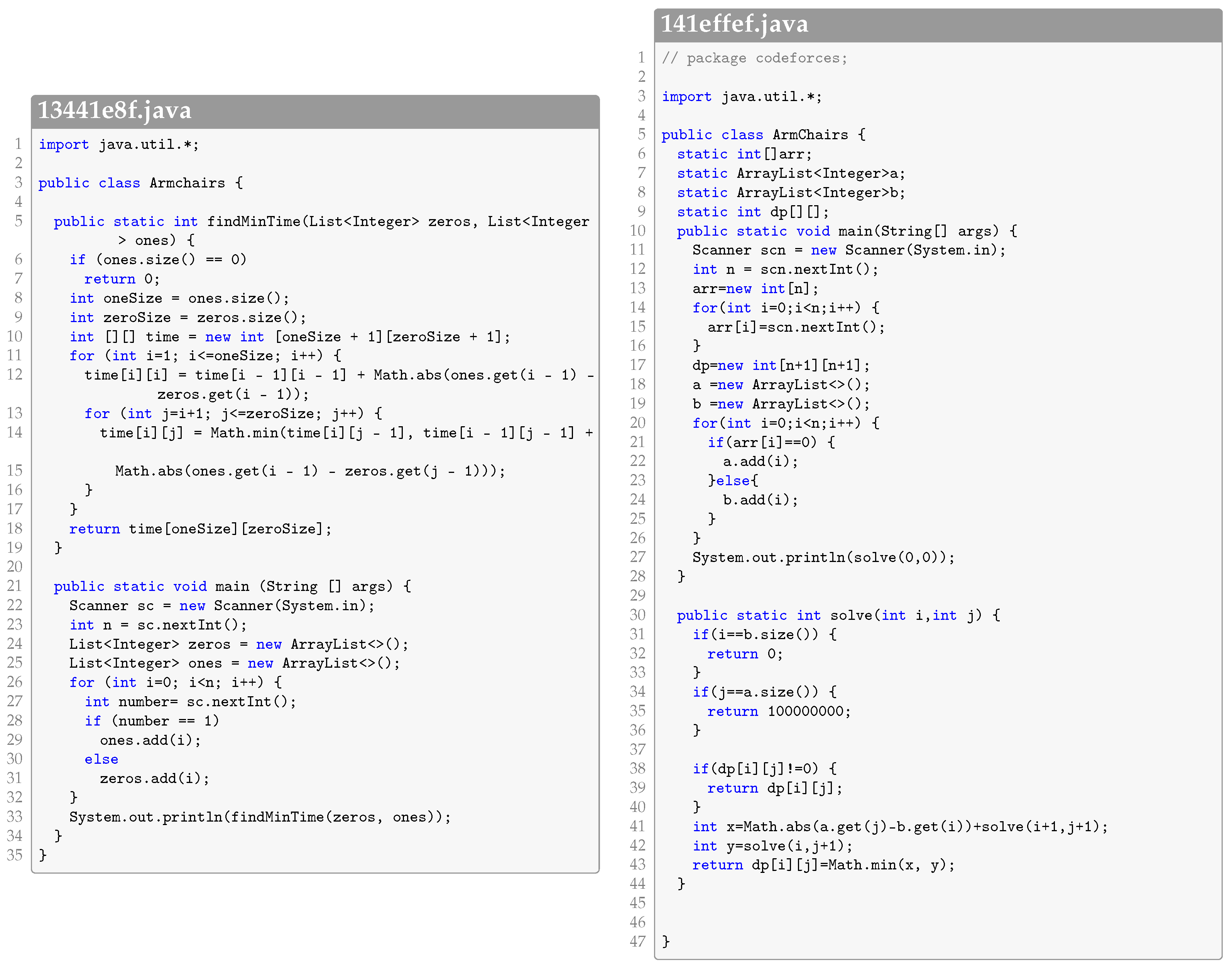
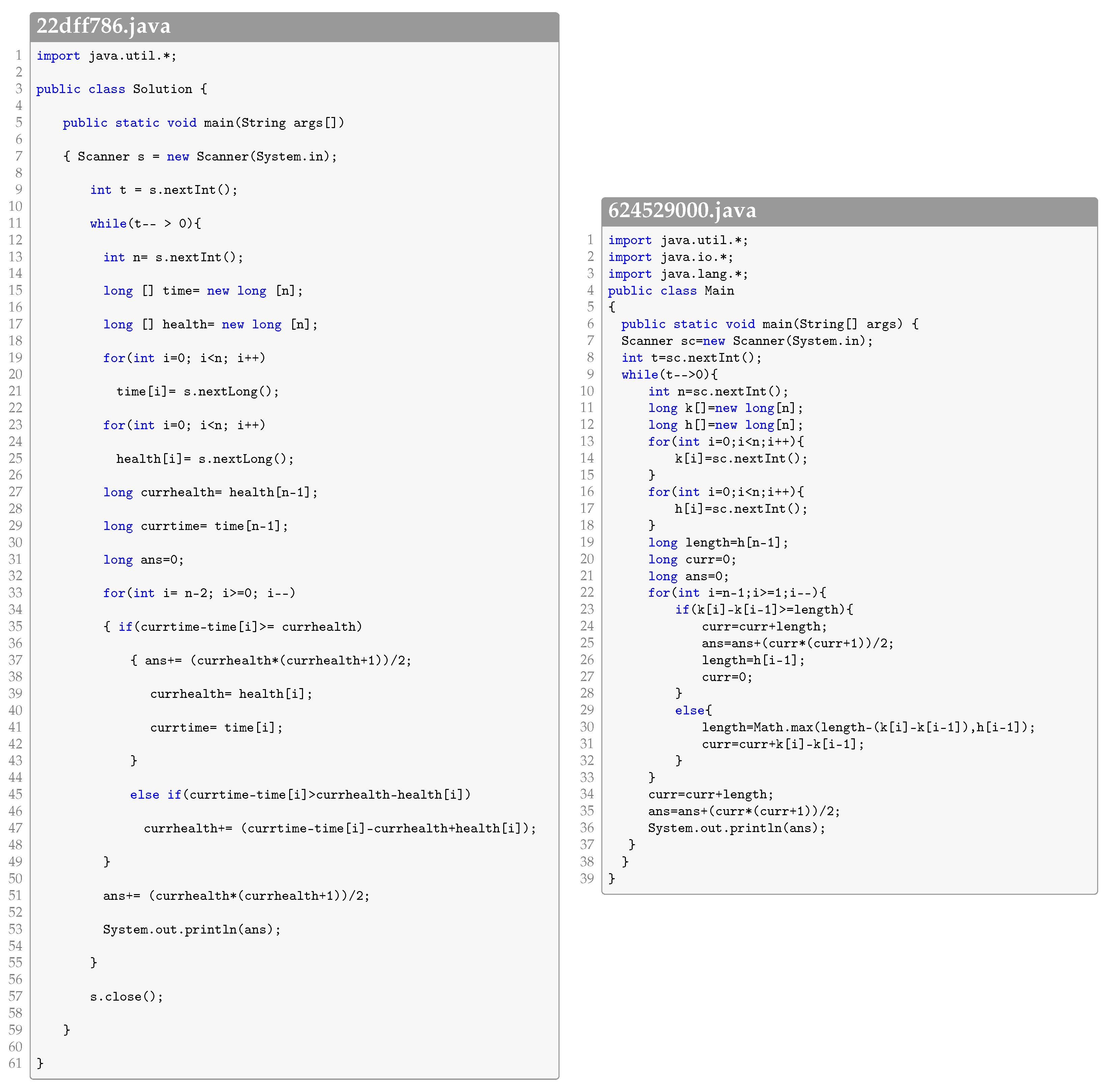
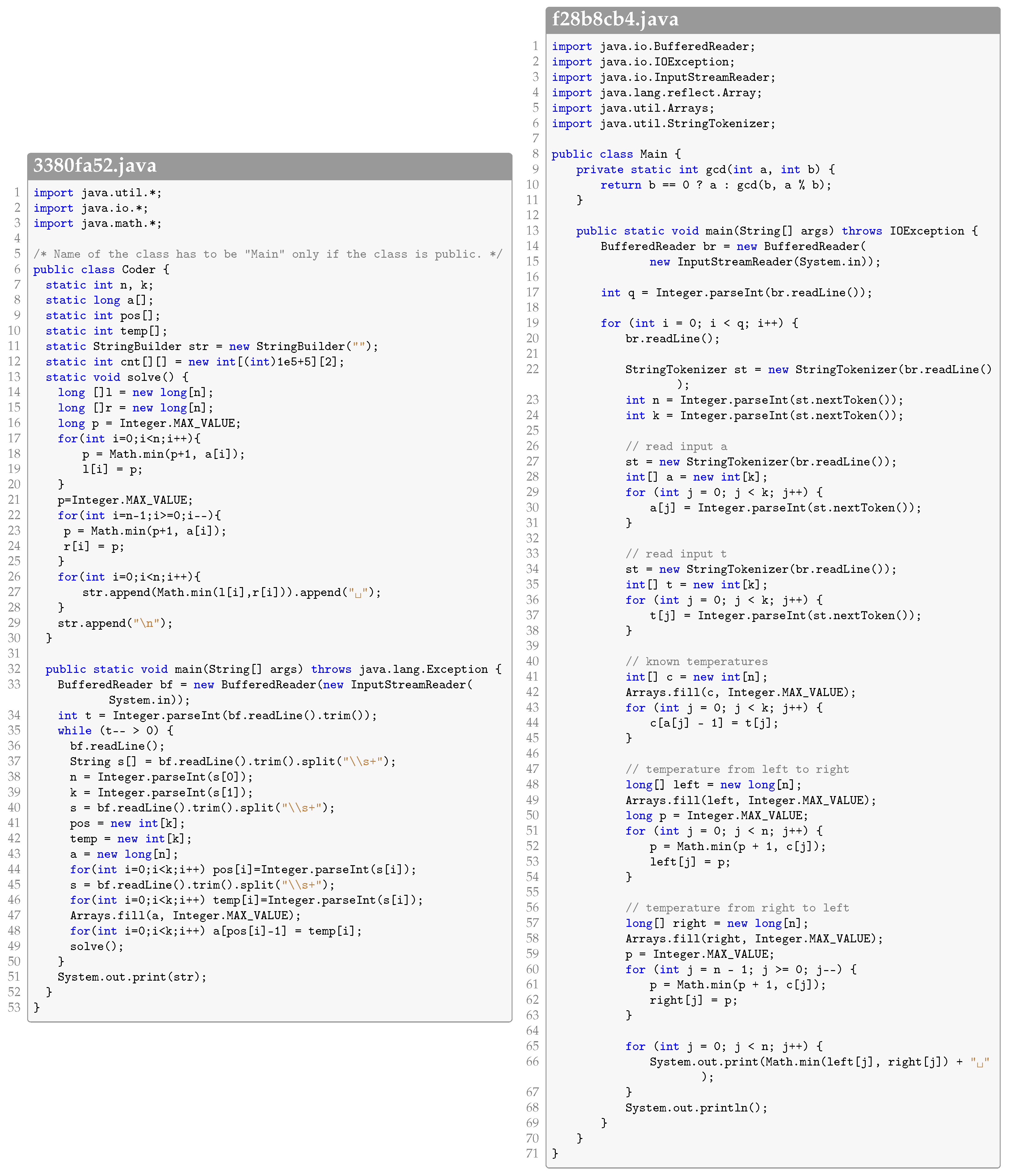
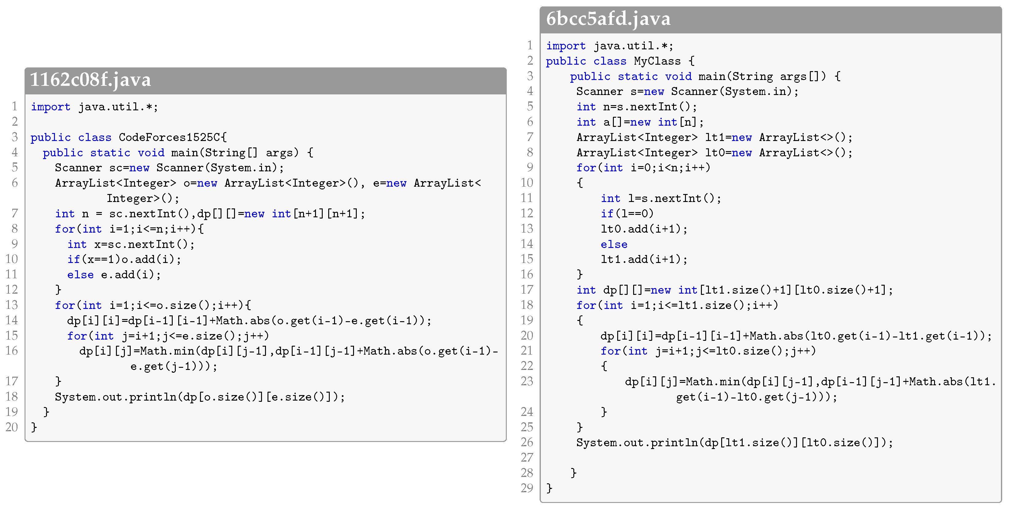
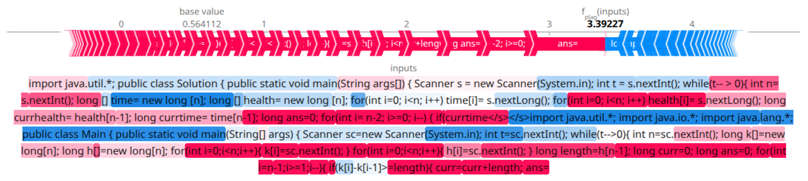
We have illustrated examples from the ConPlag1 dataset to show how plagiarism occurs at certain levels. The examples also have non-plagiarised pairs. They are used for error analysis later in the paper. They are provided in Appendix A.

2.3. PCMs

The pre-trained models follow the Transformer architecture introduced by Vaswani et al. [14], including an encoder/decoder block. There are various pre-trained models, as surveyed in [15,16], categorised in different ways. Major pre-trained language models include BERT [17], RoBERTa [18], BART [19] and T5 [20].

For the domain of AI4SE, PCMs were developed by training language models on large code corpora, such as CodeSearchNet [21]. There are several surveys covering the PCMs [2,22,23,24,25,26,27] and discussing various code understanding and generation tasks. The code models used in this study are CodeBERT [28], GraphCodeBERT [29], CodeBERTa [30], UniXcoder [31], CodeT5 [32] and PLBART [33].

Table 4. Selected PCMs and their number of parameters (in millions), model size (in MB), and base architecture.

Model	Number of Parameters	Model Size	Base Architecture
CodeBERT	125 M	499 MB	RoBERTa
GraphCodeBERT	125 M	499 MB	RoBERTa
UniXcoder	125 M	504 MB	RoBERTa
PLBART	140 M	557 MB	BART
CodeT5-Small	60 M	242 MB	T5
CodeBERTa	84 M	336 MB	RoBERTa

summarises the selected PCMs in terms of the number of parameters in millions (Ms) and model size in megabytes (MBs) of public checkpoints and base architecture. These models differ in terms of the initial pre-training data and code representation. For the classification, all models except CodeT5 and PLBART adopt the RoBERTa architecture. CodeT5 adheres to the T5 architecture, while PLBART follows the BART architecture. We select an encoder and an encoder/decoder model, as we treat the SCPC as an understanding task rather than a generation task. Furthermore, in previous surveys [2,23], encoder and encoder/decoder models consistently outperformed decoder models in all code-understanding tasks. Although prompt-based decoder models can be used to generate classes, we consider them for investigation in future work.

Fine-tuning refers to customising model parameters for a downstream task. In FFT, the full model is updated for SCPC. In PEFT, the base Transformer remains frozen and only the task-specific components are trained.

For the binary SCPC task, each model predicts two logits, one for non-plagiarised and one for plagiarised code pairs. The models are trained using cross-entropy loss. This loss compares the two logits with the true class label and penalises the model when it assigns a higher score to the wrong class. The loss is computed directly from logits; the softmax term in Equation (1) shows the mathematical form of the two-class cross-entropy.

$$\mathcal{L}=-{\displaystyle \frac{1}{N}}{\displaystyle \sum _{i=1}^N}{\displaystyle \sum _{c=0}^1}{w}_c{y}_{i,c}log\left({\displaystyle \frac{exp\left(z_{i,c}\right)}{{\sum }_{j=0}^{1}exp\left(z_{i,j}\right)}}\right)$$

(1)

In Equation (1), $z_{i,c}$ is the logit for sample i and class c, $y_{i,c}$ is the true class indicator, and $w_c$ is the class weight.

To account for class imbalance, we use class-weighted cross-entropy. The class weights are computed from the training split, or from the training fold in cross-validation, only. For each class c, the weight is set to the complement of its training-set proportion, $w_c=1-n_c/N$, where $n_c$ is the number of training samples in class c.

The two logits are produced by a task-specific CH, not by the original pre-training objective. The CH is randomly initialised from scratch, meaning that its linear weights start from random values and are learned during fine-tuning.

The CH is a lightweight two-layer feed-forward classifier. It applies dropout to the sequence representation, passes it through a dense layer with a tanh activation, applies dropout again, and uses a final linear projection to produce the two logits. For the RoBERTa-family encoder-only models, the representation is taken from the first special classification token, <s>, which plays the same role as [CLS]. For the encoder/decoder models, classification is still treated as pair classification rather than text generation. The classifier uses the model’s last hidden layer of the decoder. For the adapter-based runs, the head receives the model’s pooled sequence representation.

2.4. Adapters

There exist various PEFT techniques as surveyed in [3,34,35,36,37,38]. The aim of PEFT is to reduce the number of trainable parameters while maintaining high performance. The PEFT methods, according to Han et al. [39], can be divided into additive, selective, reparameterisation, or hybrid. Additive PEFT is where additional trainable parameters are configured while keeping the model weights intact. In selective PEFT, only a portion of the selected parameters are fine-tuned. Reparameterised PEFT converts the weight matrices into lower-dimensional matrices. Hybrid PEFT combines multiple PEFT techniques to improve performance while maintaining high efficiency.

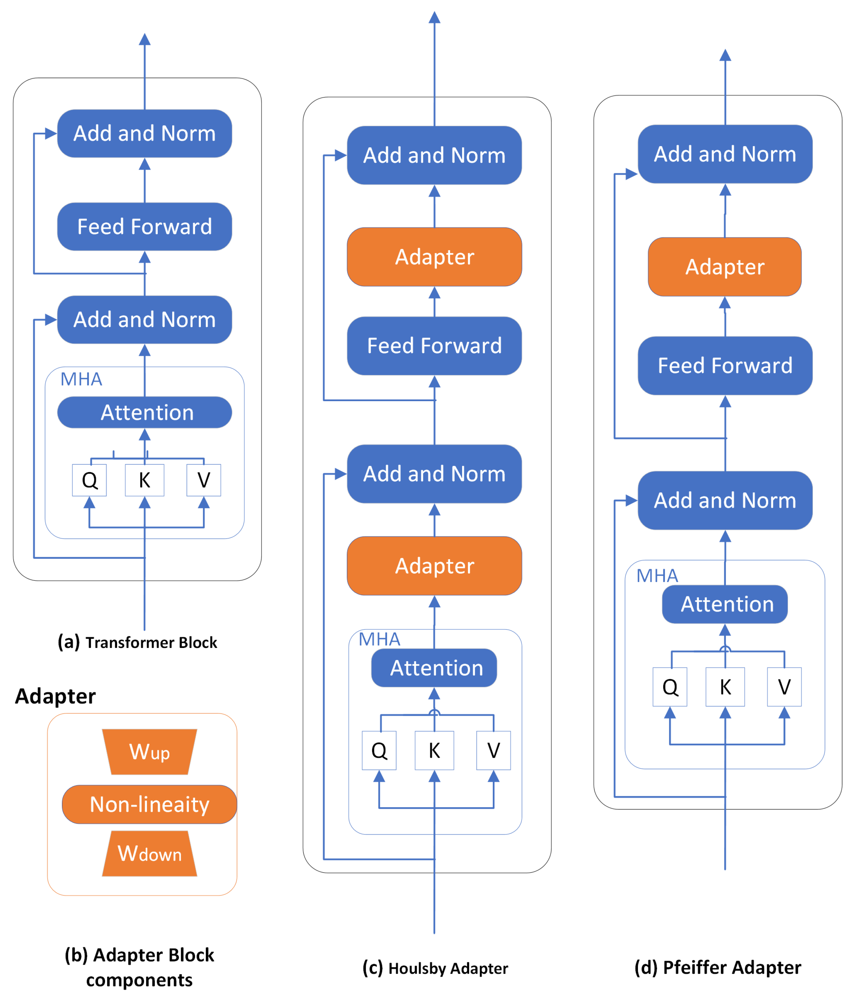
The main Transformer block of a single encoder is shown in Figure 3a. The major layers are Multi-Head Attention (MHA), add and normalisation, and feed-forward layers.

The first adapter type used in this work is the sequential adapter, in which small bottleneck modules are added inside the Transformer layers. These adapters are considered additive because they introduce new trainable parameters while leaving the original Transformer weights frozen. The Houlsby adapter [4] adds two bottleneck modules in each Transformer layer: one after the attention block and one after the feed-forward block, as in Figure 3c. Each bottleneck module contains a down-projection $\left(W_{down}\right)$, a non-linearity, and an up-projection $\left(W_{up}\right)$, as in Figure 3b. The Pfeiffer adapter [40,41] adds a single bottleneck module after the feed-forward block, as in Figure 3d. It therefore uses fewer adapter modules than Houlsby. Mathematically, the output of the adapter is as in Equation (2), where h represents a hidden state. The hidden state is first projected down, transformed by a non-linear function, f, projected back up, and then combined with the residual connection, r.

$$h\leftarrow W_{up}·f(W_{down}·h)+r$$

(2)

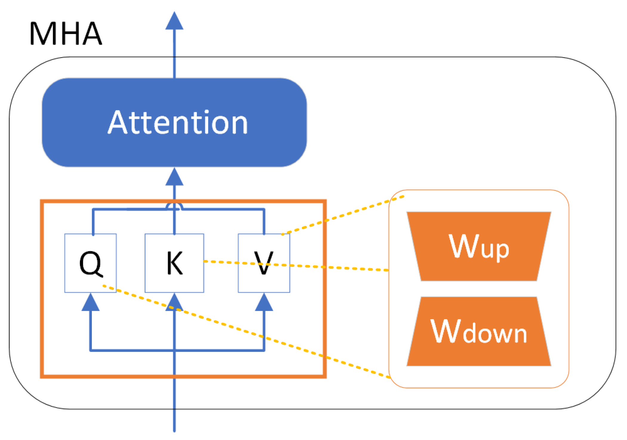
Another PEFT technique is LoRA, which focuses on the MHA block [6]. This adapter decomposes the weight matrices (Query, Key and Value) into two smaller matrices $(W_{up}$ and $W_{down}$) as per Figure 4. LoRA is a reparameterisation method for PEFT that decomposes the initial weight matrix into two smaller matrices and then merges them with the initial weight matrix $W_0$, as per Equation (3).

$$h\left(x\right)=W_{0}X+\Delta W_0=W_{0}X+\left(W_{down}{W}_{up}\right)X$$

(3)

The PEFT experiments use the same class-weighted cross-entropy objective described above. The trainable task-specific parameters include the CH and the active adapter parameters, namely the bottleneck modules in sequential adapters or the low-rank matrices in LoRA. The CH has its own parameters and does not share weights with the adapters. Both are optimised simultaneously for the same classification objective. Bottleneck adapter weights are randomly initialised. For LoRA, the A low-rank matrix is initialised from a Kaiming uniform distribution and the B matrix is initialised to zero, and they are learned during fine-tuning [6].

Houlsby and Pfeiffer adapters add bottleneck modules to each Transformer layer [4,40,42]. In contrast, LoRA inserts trainable low-rank matrices into the attention projections and can be merged back into the base weights for inference [42]. We select these two types of adapters because sequential bottleneck adapters were among the first PEFT methods and currently serve as baselines for newer methods. LoRA is one of the most widely used adapters in NLP due to its efficiency and ease of use.

Sequential Bottleneck Adapters vs. LoRA

Sequential bottleneck adapters introduce additional inference cost because they add extra feed-forward bottleneck modules to each Transformer layer. They may also require more trainable parameters than LoRA, depending on the selected bottleneck size and LoRA rank. In contrast, LoRA adds trainable low-rank matrices to existing weight matrices. Therefore, its additional inference cost can be removed when the LoRA weights are merged with the original model weights.

Mathematically, let $d_m$ denote the model hidden size, $d_b$ the adapter bottleneck dimension, and r the LoRA rank. The complexity and number of trainable parameters per layer [35,37] are summarised in

Table 5. Comparison between sequential adapters and LoRA regarding number of trainable parameters per layer, inference cost and complexity.

Method	Number of Parameters	Inference Cost	Complexity
Sequential Adapters	$2\times \left(2d_m{d}_b\right)$	Extra bottleneck FFN	$\mathcal{O}\left(d_m{d}_b\right)$
LoRA	$2\times \left(2d_{m}r\right)$	None if merged	$\mathcal{O}\left(d_{m}r\right)$

. For a sequential bottleneck adapter, the down-projection and up-projection matrices have sizes $d_m\times d_b$ and $d_b\times d_m$, respectively. Thus, one adapter module adds approximately $2d_m{d}_b$ trainable parameters, excluding biases. If two adapter modules are inserted per Transformer layer, the parameter count becomes $2\times \left(2d_m{d}_b\right)$. For LoRA, one adapted weight matrix with input and output dimensions equal to $d_m$ adds two low-rank matrices with approximately $2d_{m}r$ trainable parameters. If LoRA is applied to two projection matrices per layer, the parameter count becomes $2\times \left(2d_{m}r\right)$.

2.5. Experimental Setup

The experiments in this work included FFT of six PCMs: CodeBERT, GraphCodeBERT, UniXcoder, CodeBERTa, CodeT5, and PLBART. First, these models were fully fine-tuned. They were then fine-tuned using three PEFT methods: Houlsby, Pfeiffer, and LoRA. The experiments used a batch size of 16 and a maximum token length of 512.

2.5.1. Input Formatting and Tokenisation

Each dataset instance consists of two source code snippets and one binary label. To split the code snippets into tokens, we used model-based tokenisers. Tokenisers break text or code into smaller parts called tokens so that models can turn them into numbers. Instead of splitting by spaces, they use subword units, which helps with rare words and long variable names. For example, the word calculateAverageScore might become calculate, Average, Score. This makes it easier for models to understand patterns even if they have not seen the full word before. Each token is then mapped to an ID in the model vocabulary. Tokenisers also handle padding, truncation, and special symbols such as <s> or [SEP] to show where a sequence starts and ends. The two main methods used with pre-trained models are Byte Pair Encoding (BPE) [43] and SentencePiece [44]. BPE merges frequent character pairs step by step to build a fixed vocabulary, while SentencePiece learns subwords directly from raw text and does not rely on spaces.

For models such as CodeBERT, GraphCodeBERT, and CodeBERTa, the tokeniser is based on BPE, originally from RoBERTa. It takes both source code and natural language and splits them into subwords using a shared fifty-thousand-word vocabulary. For example, public static void main becomes public, static, void, main, but a long variable like getStudentDetailsFromDB might split into get, Student, Details, From, DB.

UniXcoder starts with the same RoBERTa-style BPE but extends it to handle multiple input types, including natural language, source code, and abstract syntax tree information. It adds special tokens such as [FUNC], [CLS_NL], and [CLS_PL] to tell the model what kind of input it is reading. It also uses extra embeddings to mark structure, such as data flow between variables. For example, if a function like int add(int a, int b) { return a + b; } is given, UniXcoder keeps the same subwords (int, add, (, a, ,, b, ), {, return, a, +, b, ;, }), but also encodes how a and b are connected in the code flow.

PLBART and Small CodeT5 use SentencePiece tokenisers. SentencePiece looks at text as a continuous stream and learns subwords without using spaces as boundaries. For instance, print("HelloWorld") might become print, (", Hello, World, "). PLBART uses a SentencePiece model with around fifty thousand tokens shared between encoder and decoder, which helps with multilingual and multi-language training. CodeT5 also uses SentencePiece but adds special tokens such as <extra_id_0> and <extra_id_1> to handle tasks where part of the code is masked or missing.

In the FFT and PEFT experiments, the source code is tokenised as provided by the selected dataset version. This means that comments, imports, identifiers, keywords, operators, string literals, and white-space-dependent formatting are preserved before tokenisation, except in the template-free ConPlag version, where the dataset authors had already removed the template code. For each code pair, the model input is limited to 512 tokens. Because each instance contains two source code fragments, this token context is shared between the two fragments, with each fragment receiving approximately half of the available token space. In addition, the tokeniser inserts the model-specific special tokens needed to encode a paired input, such as classification and separator tokens. These special tokens count toward the 512-token limit, leaving slightly fewer positions for the source code tokens themselves. If a code fragment exceeds its allocated token budget, it is truncated before being passed to the model. Additional preprocessing is evaluated separately in Section 3.2.2; in that experiment, comments, imports, and repeated spaces are removed to reduce the number of tokens before model tokenisation.

2.5.2. Hyperparameter Search

Hyperparameter optimisation was performed as an exhaustive grid search over learning rates only. In the literature, learning rate has the most impact on fine-tuning [45]. The batch size, adapter reduction factor, LoRA rank and scaling factor, and dropout settings were fixed to keep the FFT and PEFT comparisons tractable and comparable across six models and four datasets under the available GPU budget. Furthermore, we aim to have a similar search space for both fine-tuning types. Since adapters typically require a higher learning rate than FFT, we used learning rates of [$1\times {10}^{-4}$, $2\times {10}^{-4}$, $3\times {10}^{-4}$, $5\times {10}^{-4}$] for adapters and [$1\times {10}^{-5}$, $2\times {10}^{-5}$, $3\times {10}^{-5}$, $5\times {10}^{-5}$] for FFT. For each model, dataset, and fine-tuning strategy, the learning rates were trained under the same training split, and validation $F_1$ was used as the selection criterion. The testing set in cross-validation was used only for final evaluation after the configuration was selected. The maximum number of epochs was set to 15, and early stopping was used to prevent overfitting when validation $F_1$ declined, as the decision was based on validation $F_1$. Training used the AdamW optimiser [46] with a linear learning rate schedule, using the default momentum parameters ${\beta }_1=0.9$, ${\beta }_2=0.999$, and $ϵ={10}^{-8}$. Other parameters include a batch size of 16. Weight decay was set to zero in the AdamW optimiser, so no weight decay regularisation was applied. The dropout rate was not manually set to zero or tuned; the models used their default dropout settings, including the classification-head dropout where applicable. No label smoothing or focal-loss variant was used. The default adapter reduction factor was 16 for Houlsby and Pfeiffer. For LoRA, $r=\alpha =8$. All experiments were conducted on an Nvidia RTX 4090 GPU with 24 GB of memory. The main library used for the pre-trained models was Hugging Face Transformers [30], while AdapterHub [5,42] was used for adapters.

2.6. Evaluation

Classification performance can be assessed using several evaluation metrics [47]. In this study, a positive prediction indicates detected plagiarism, whereas a negative prediction indicates non-plagiarism. Therefore, True Positive ($TP$) denotes correctly identified plagiarism, False Positive ($FP$) denotes incorrectly identified plagiarism, also known as a false alarm, True Negative ($TN$) denotes correctly identified non-plagiarism, and False Negative ($FN$) denotes missed plagiarism. We focus on $FP$ and $FN$ in the results because false alarms and missed plagiarism have different practical implications.

Precision, recall, and the $F_1$ score are calculated as follows:

$$Precision\left(P\right)={\displaystyle \frac{TP}{TP+FP}}$$

(4)

$$Recall\left(R\right)={\displaystyle \frac{TP}{TP+FN}}$$

(5)

$$F_1=2·{\displaystyle \frac{Precision·Recall}{Precision+Recall}}$$

(6)

Since the classes are imbalanced, accuracy is not used as the main evaluation metric. We report precision and recall to separate false alarms from missed plagiarism, and use $F_1$ as the primary ranking metric because it provides a balanced summary of both quantities. This also keeps the comparison consistent across the PCMs, adapters, JPlag, and Dolos.

3. Results

This section presents the experimental results and several efficiency comparison metrics. The experimental results are reported using both a random single split and k-fold cross-validation.

3.1. Random Single Split Results

The random single split is used for exploratory analysis, hyperparameter optimisation, and error analysis. We use a stratified 70%/15%/15% split for training, validation, and testing, respectively, to maintain a similar class distribution across partitions. The validation set is used for hyperparameter selection, while the metrics are reported on the testing set. The split composition is shown in

Table 6. Number of training, validation, and testing instances per dataset in the random single split. ConPlag1 and ConPlag2 share the same split counts.

Dataset	Split	Plagiarised	Non-Plagiarised	Total
ConPlag1/ConPlag2	Train	176	461	637
	Validation	38	99	137
	Test	42	95	137
IR-Plag	Train	257	65	322
	Validation	55	14	69
	Test	54	15	69
Progpedia-19	Train	64	1437	1501
	Validation	12	310	322
	Test	15	307	322

. The main performance conclusions are based on cross-validation. However, the single split remains beneficial because it preserves validation and test splits for hyperparameter selection and detailed qualitative analysis.

Table 7. $F_1$ scores per fine-tuning method across four datasets in the random single split.

Dataset	Model	FFT	Houlsby	Pfeiffer	LoRA
ConPlag1	CodeBERT	0.8046	0.7179	0.6098	0.6250
	GraphCodeBERT	0.8235	0.8049	0.8333	0.6869
	UniXcoder	0.8810	0.8276	0.7619	0.7736
	CodeBERTa	0.7857	0.7742	0.7586	0.7660
	PLBART	0.9176	0.8000	0.9398	0.7907
	CodeT5	0.7959	0.9000	0.7778	0.7723
ConPlag2	CodeBERT	0.8293	0.7234	0.7527	0.6512
	GraphCodeBERT	0.7654	0.7727	0.7234	0.6508
	UniXcoder	0.8387	0.8095	0.7917	0.7835
	CodeBERTa	0.8049	0.8095	0.8101	0.8293
	PLBART	0.9268	0.8966	0.9195	0.8864
	CodeT5	0.7451	0.8000	0.7473	0.8000
IR-Plag	CodeBERT	0.9908	0.9725	0.9636	0.9550
	GraphCodeBERT	0.9907	1.0000	0.9818	0.9908
	UniXcoder	1.0000	1.0000	1.0000	0.9818
	CodeBERTa	0.9818	0.9818	0.9818	0.9908
	PLBART	1.0000	0.9908	1.0000	0.9908
	CodeT5	0.9286	0.8852	0.9076	0.9725
Progpedia-19	CodeBERT	1.0000	1.0000	1.0000	1.0000
	GraphCodeBERT	1.0000	1.0000	1.0000	1.0000
	UniXcoder	1.0000	0.9677	1.0000	1.0000
	CodeBERTa	1.0000	0.9677	0.9677	0.9677
	PLBART	1.0000	1.0000	1.0000	1.0000
	CodeT5	0.9677	0.9091	0.9677	0.9375

reports the $F_1$ scores for the selected PCMs with FFT and the adapters across ConPlag1, ConPlag2, IR-Plag, and Progpedia-19.

3.1.1. Full Fine-Tuning of PCMs

The FFT results are available in Table 7. For the IR-Plag dataset, FFT gave robust results. UniXcoder and PLBART reached an $F_1$ score of 1.0000. CodeBERT and GraphCodeBERT followed at around 0.9908, CodeBERTa reached 0.9818, and CodeT5 had the lowest score at 0.9286. The errors in FFT were mainly due to cases involving long comments or simple introductory Java printing examples. These results show that FFT handled the dataset well, and most models produced near-perfect predictions. For the Progpedia-19 dataset, FFT produced $F_1$ scores of 1 for all models except CodeT5. The models except CodeT5 classified every test instance correctly, which reflects the simplicity of the dataset and the apparent differences between the classes. CodeT5 showed one $FP$. This case showed higher similarity at the start of the code, leading the model to treat it as plagiarised. Apart from this single error, FFT achieved near-perfect $F_1$ performance across the dataset.

For the ConPlag1 dataset, PLBART achieved the highest FFT score at 0.9176, followed by UniXcoder at 0.8810 and GraphCodeBERT at 0.8235. The lowest FFT score in this dataset was obtained from CodeBERTa with a score of 0.7857. For the ConPlag2 dataset, PLBART again ranked first with 0.9268, followed by UniXcoder at 0.8387 and CodeBERT at 0.8293. CodeT5 achieved the lowest FFT score on this dataset, 0.7451. We conduct an error analysis of these two datasets in the later subsections.

Finding 1: PCMs are robust given high-quality training data, resulting in high $F_1$ scores on the easier IR-Plag and Progpedia-19 datasets and lower scores on the more challenging ConPlag datasets.

3.1.2. PEFT

The results of merging the adapters to the PCMs, in terms of evaluation metrics, are presented in Table 7.

For the IR-Plag dataset, FFT already produced robust results. Several models matched the FFT score of 1, including GraphCodeBERT with Houlsby (higher than FFT), UniXcoder with sequential adapters, and PLBART with the Pfeiffer adapter. CodeBERTa with LoRA and CodeT5 with LoRA also improved, reaching 0.9908 and 0.9725, respectively. CodeBERT was the only model in which all adapters reduced performance compared with FFT. In contrast, the other models kept their $F_1$ performance or matched FFT. For the Progpedia-19 dataset, FFT and PEFT scored 1 for almost all models. The adapters did not reduce $F_1$ except for CodeBERTa. The dataset is simple, and both FFT and PEFT reached perfect predictions for all models except CodeT5 and CodeBERTa.

For the ConPlag1 dataset, several models benefited from the use of adapters. PLBART with the Pfeiffer adapter achieved the highest $F_1$ score of 0.9398, surpassing FFT. CodeT5 with Houlsby also improved and reached 0.9000. GraphCodeBERT with the Pfeiffer adapter reached 0.8333, higher than its FFT value. CodeBERTa, CodeBERT, and UniXcoder did not improve over FFT on ConPlag1. For the ConPlag2 dataset, PLBART with the Pfeiffer adapter achieved the highest adapter score at 0.9195, which remained below PLBART’s FFT score of 0.9268. CodeBERTa with LoRA reached 0.8293, higher than its FFT score. CodeT5 with Houlsby and LoRA both reached 0.8000, and GraphCodeBERT with Houlsby improved to 0.7727. UniXcoder and CodeBERT did not benefit from the adapters in this dataset.

An observation is that the smaller models, CodeBERTa and CodeT5, benefited more and mostly achieved better results with adapters than with Full Fine-Tuning. This may be due to having even fewer parameters to fine-tune, making the models more manageable and less prone to overfitting.

Finding 2: Merging adapters with the PCMs led to better or similar $F_1$ scores compared to FFT. The main exceptions were CodeBERT on IR-Plag and both ConPlag datasets, and UniXcoder across the ConPlag datasets.

3.1.3. Error Analysis

In this subsection, we investigate the plagiarism cases or levels that the PCMs or adapters successfully captured, and those that the model failed to capture. The analysis uses the correct positive predictions over the total number of plagiarised test pairs in each level, following the single-split results.

In ConPlag1, all selected FFT and adapter runs detected the L1 cases. The remaining errors were concentrated in L2–L6. For FFT, CodeBERT and GraphCodeBERT each produced 7 $FNs$, UniXcoder produced 5, CodeBERTa produced 9, and PLBART and CodeT5 each produced 3. The best adapters did not uniformly reduce missed positives: CodeBERT increased to 14 $FNs$, GraphCodeBERT stayed at 7, UniXcoder increased to 6, CodeBERTa decreased to 6, PLBART stayed at 3, and CodeT5 increased to 6. This shows that adapter improvements in $F_1$ are related to reducing $FPs$, not only from detecting more plagiarised pairs.

In ConPlag2, all selected runs again detected the L1 cases, while the harder levels were mainly L3–L6. FFT produced 8 $FNs$ with CodeBERT, 11 with GraphCodeBERT, 3 with UniXcoder, 9 with CodeBERTa, and 4 each with PLBART and CodeT5. The best adapters reduced missed positives for CodeBERT, GraphCodeBERT, CodeBERTa, PLBART, and CodeT5, but increased UniXcoder’s missed positives from 3 to 8. PLBART and CodeT5 were the strongest adapters on this per-level view, each missing only 2 positives on ConPlag2.

The L4 cases in which most models failed to capture involve either creating a new function or placing it at the beginning or end of a long code block. Therefore, the instances in which the models or adapters consistently failed to capture were those in which plagiarism occurred in lengthy code, due to the pre-trained models’ 512-token limit. Furthermore, adding unused functions at the beginning of the file results in an $FN$ with the PCMs.

Finding 3: The PCMs fail to capture plagiarism occurring at the end of lengthy code snippets exceeding their maximum length of 512. They also fail to capture the obfuscated, unnecessary functions added to the beginning of the code.

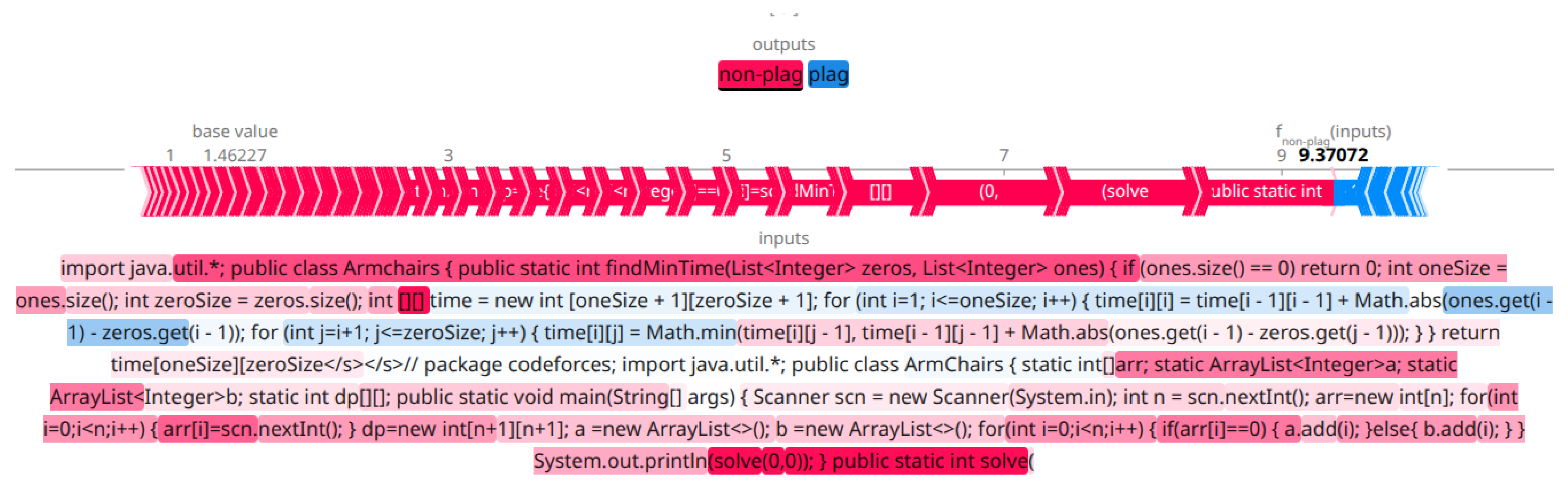
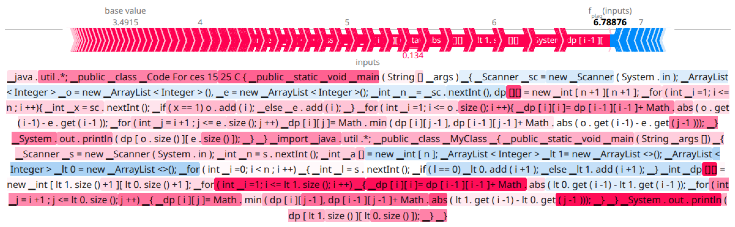
Detailed qualitative code pair examples that support Finding 3 are provided in Appendix A.

3.1.4. FFT vs. PEFT

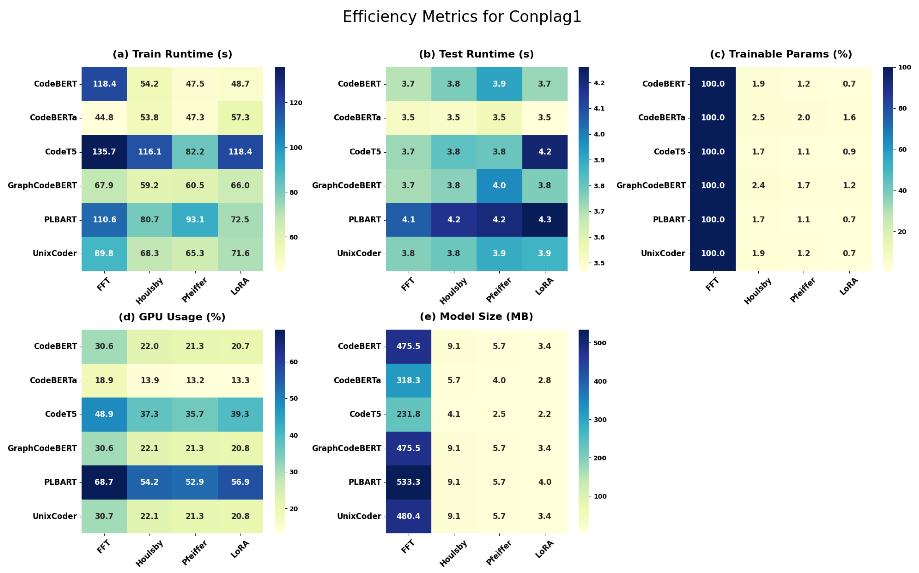
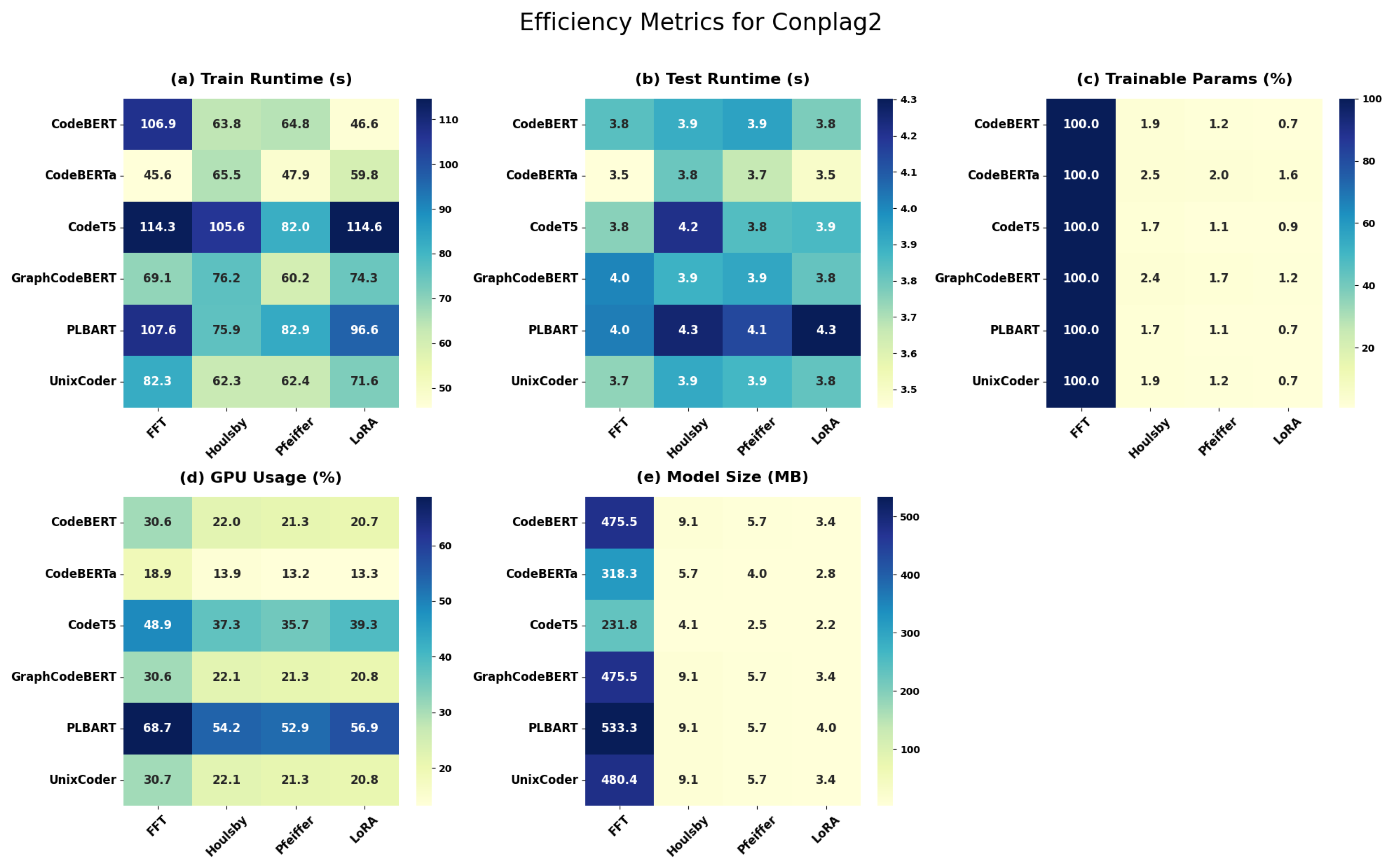
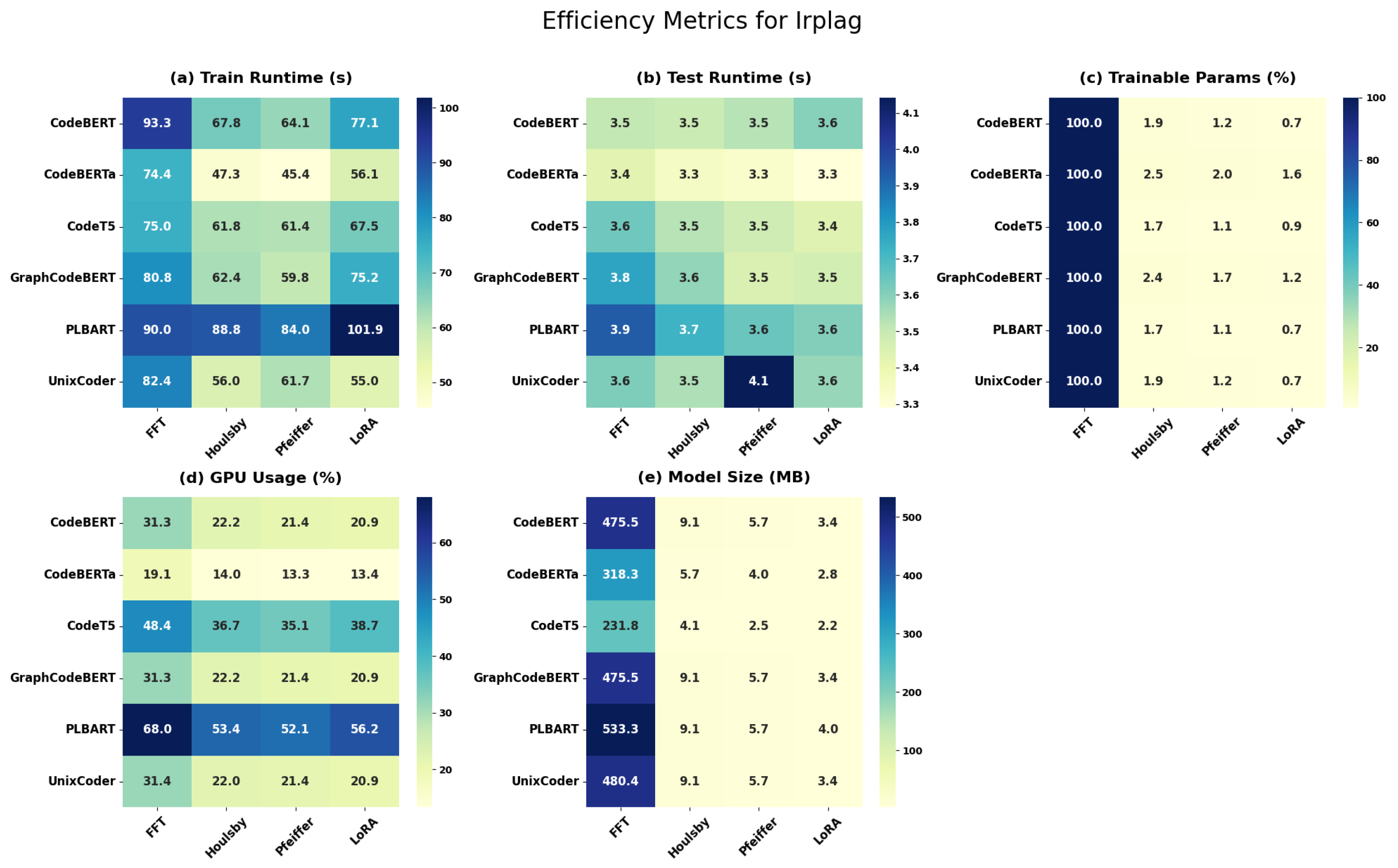
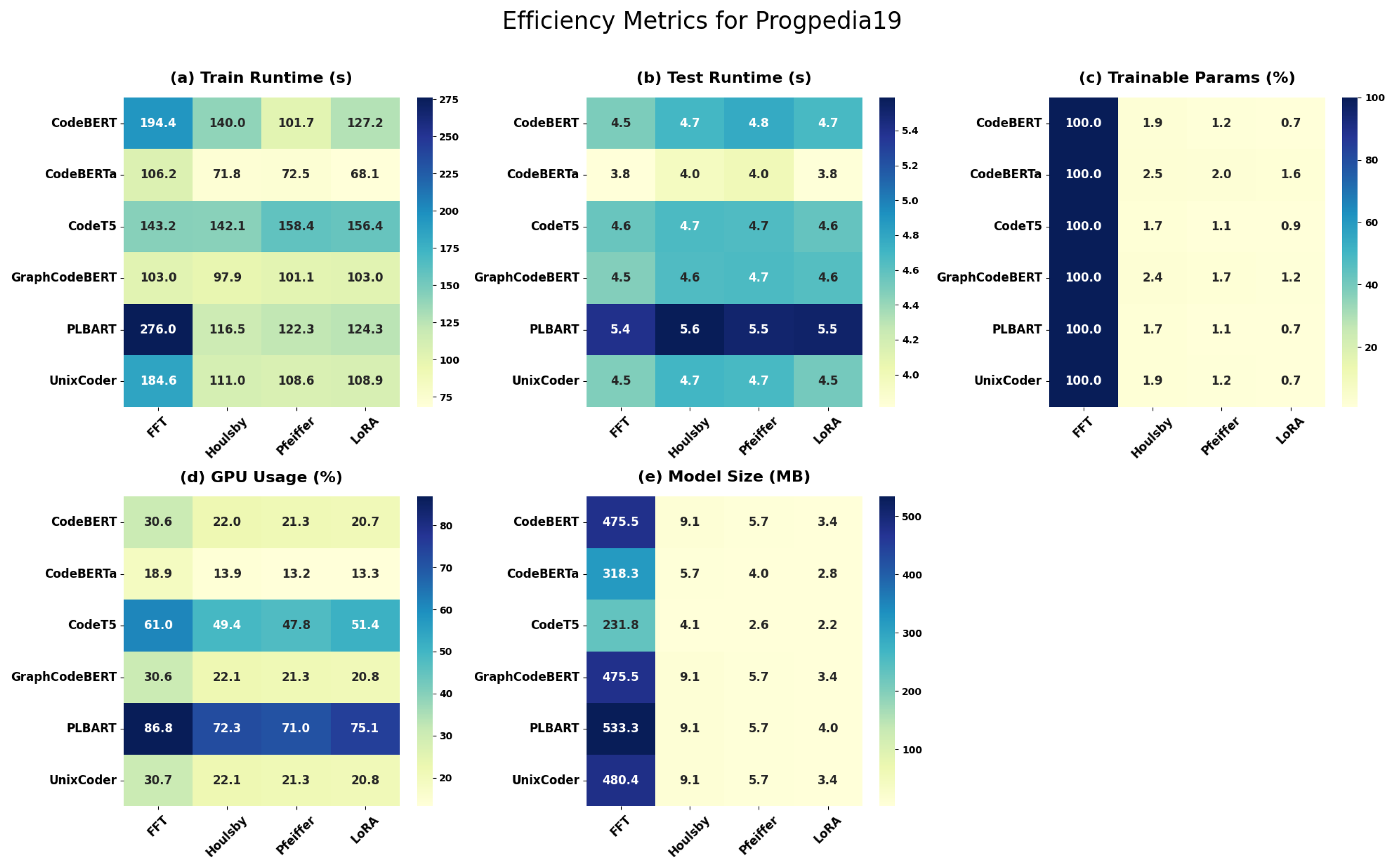
During the experimental phase, various efficiency metrics were monitored, including training time, inference time, GPU usage, and the number of trainable parameters for all pre-trained models and adapters across both dataset versions. We report efficiency metrics and comparisons across the ConPlag raw dataset, as shown in Figure 5. For the other datasets, the efficiency metrics are available in Appendix D. They lead to the same conclusions.

Model/adapter size and trainable parameters percentage: Regarding the PCMs, their public checkpoint size and number of parameters were previously presented in Table 4. The fine-tuned model sizes and adapter sizes for the raw dataset are illustrated in Figure 5e. The percentages of trainable parameters for all the models for the raw dataset are presented in Figure 5c. The sizes of fine-tuned models are slightly different from the public checkpoints. CodeBERT, GraphCodeBERT, and UniXcoder have comparable fine-tuned model sizes of approximately 480 MB, with approximately 125M parameters. PLBART has the largest fine-tuned model size, at 534 MB, with 140 M trainable parameters. CodeBERTa measures 320 MB and has 84 M configurable parameters. Among the selected models, CodeT5-small is the smallest, with a size of 234 MB and 60 M parameters. The fine-tuned model sizes in Figure 5e are slightly different from the public checkpoint sizes in Table 4. In FFT, all parameters require adjustment, resulting in 100% trainable parameters.

For the adapters, the Houlsby adapter is the largest and highest in percentage of trainable parameters, followed by Pfeiffer, and then LoRA. The size of the Houlsby adapter, including the CH, is 9.1 MB for CodeBERT, GraphCodeBERT, PLBART, and UniXcoder, whereas it is 5.7 MB for CodeBERTa and 4.1 MB for CodeT5. The parameter count percentage for Houlsby ranges from 1.7% for PLBART and CodeT5 to 2.5% for CodeBERTa. In the Pfeiffer adapter, the model size ranges from 2.5 MB to 5.7 MB, and the percentage of trainable parameters ranges from 1.1% to 2.0%. For LoRA, the size is 2.2 MB for CodeT5 and 4.0 MB for PLBART, and the trainable parameters range from 0.7% to 1.6%. When merged, the adapter size is added to the model size.

Assuming k tasks, model size m, and adapter size n, FFT requires approximately $km$ storage, whereas adapters require approximately $m+kn$ storage when a single base model is shared. This is advantageous when dealing with multiple tasks and multiple pre-trained models. For instance, storing four CodeBERT FFT checkpoints would require approximately $4\times 475.5=1902$ MB, whereas one CodeBERT base model plus four LoRA adapters of about 3.4 MB each would require approximately $475.5+(4\times 3.4)=489.1$ MB. However, for a single-task setting, additional storage is still required to save the adapters for merging with the pre-trained model. Overall, compared to FFT, adapter size is reduced by around 98% to 99.5%, while the percentage of trainable parameters is reduced by around 97.5% to 99.3%, depending on the model and adapter type.

GPU Usage percentage: During the experiments, we monitored the GPU usage percentage during training as per Figure 5d. FFT surpasses PEFT in GPU usage and is more resource-intensive. The highest GPU usage was with PLBART, reaching 68.7%. It was reduced to 52.9% in Pfeiffer, with higher $F_1$ performance. The minimum GPU usage for FFT was 18.9% with CodeBERTa, and it decreased to 13.2% with a reduction of around 30% with Pfeiffer and LoRA. CodeBERT, GraphCodeBERT, and UniXcoder showed relative reductions of approximately 28%–32%, while CodeBERTa had the lowest absolute GPU usage. Hence, all adapters use less GPU than FFT.

Training and prediction time: Since we used a validation set with early stopping, the training time across the experiments was not consistent. Overall, adapters required less training time than FFT. However, adapters may need more training epochs to converge than FFT, whereas they achieve faster training in the same number of epochs. For the prediction time, since the testing set was small, the difference between FFT and adapters was slight. Overall, in the experiments, adapters required slightly longer inference times than FFT, with LoRA having the lowest inference cost among the adapters.

Finding 4: Full fine-tuning exhibits lower inference costs, while adapters show advantages in GPU usage and number of trainable parameters.

3.1.5. Comparison with SCPDTs

The two current open-source SCPDTs used in this study are JPlag [48] and Dolos [49]. Both are unsupervised similarity-based tools, whereas the fine-tuned PCMs are supervised classifiers that require labelled training pairs. Therefore, the comparison is intended to show the empirical difference between these two deployment paradigms on the selected datasets, not to imply that supervised models are a direct replacement for unsupervised tools in every setting. We optimise parameters for both tools using only the training and validation data and then report their performance on the testing set. The parameters and best parameters used for both JPlag and Dolos are available in Appendix B. The pairs are labelled as plagiarised or not based on a threshold; if the similarity exceeds this threshold, the pairs are labelled plagiarised. We experimented with thresholds ranging from 0.01 to 0.99 and selected the best threshold based on the validation data. The test set is not used during parameter or threshold selection.

The results can be seen in

Table 8. Comparison between plagiarism-detection tools and PLBART (FFT and PEFT), across four datasets, in terms of precision, recall, and $F_1$ scores, in the single random split.

IR-Plag
Tool/Model	P	R	${\mathbf{F}}_{\mathbf{1}}$	# FPs	# FNs
JPlag	0.7925	0.7778	0.7850	11	12
Dolos	0.8136	0.8889	0.8496	11	6
PLBART (FFT)	1.0000	1.0000	1.0000	0	0
PLBART (Pfeiffer)	1.0000	1.0000	1.0000	0	0
ConPlag1
Tool/Model	P	R	${\mathbf{F}}_{\mathbf{1}}$	# FPs	# FNs
JPlag	0.6939	0.8095	0.7473	15	8
Dolos	0.5000	0.9286	0.6500	39	3
PLBART (FFT)	0.9070	0.9286	0.9176	4	3
PLBART (Pfeiffer)	0.9512	0.9286	0.9398	2	3
ConPlag2
Tool/Model	P	R	${\mathbf{F}}_{\mathbf{1}}$	# FPs	# FNs
JPlag	0.6379	0.8810	0.7400	21	5
Dolos	0.6786	0.9048	0.7755	18	4
PLBART (FFT)	0.9500	0.9048	0.9268	2	4
PLBART (Pfeiffer)	0.8889	0.9524	0.9195	5	2
Progpedia-19
Tool/Model	P	R	${\mathbf{F}}_{\mathbf{1}}$	# FPs	# FNs
JPlag	0.8824	1.0000	0.9375	2	0
Dolos	0.9375	1.0000	0.9677	1	0
PLBART (FFT)	1.0000	1.0000	1.0000	0	0
PLBART (Pfeiffer)	1.0000	1.0000	1.0000	0	0

. For IR-Plag, the best-performing model in the experiments, PLBART with FFT and Pfeiffer, achieved higher scores than the tools across all metrics, achieving a score of 1. JPlag had 11 $FPs$ and 12 $FNs$ (across L4 to L6). The similarity scores for some of the $FNs$ are low (<0.22), which led to their labelling as negatives. This indicates an issue with JPlag at the levels L5 and L6. A quarter of the $FPs$ had a similarity value (>0.97). Dolos had 6 $FNs$ related to cases L4 to L6, with similarity scores below 0.23, while correctly detecting other plagiarism levels. For the Progpedia-19 dataset, several pre-trained models yielded an $F_1$ score of 1. JPlag had two $FPs$ related to the addition of extra or obfuscated code, and Dolos had a single $FP$ related to extra added functions. The plagiarism modifications were simple and easy to capture. For the ConPlag datasets, PLBART with both FFT and PEFT achieved higher $F_1$ scores than both tools. For the raw dataset, Dolos yielded 39 $FPs$ and 3 $FNs$, with $FNs$ primarily occurring at plagiarism levels L3 to L5. In contrast, JPlag produced 15 $FPs$ and 8 $FNs$, with failures concentrated in plagiarism levels L4 to L6. For the template-free dataset, Dolos yielded 18 $FPs$ and 4 $FNs$, with $FNs$ primarily occurring at plagiarism levels L3 to L5. In contrast, JPlag produced 21 $FPs$ and 5 $FNs$, with failures spanning plagiarism levels L3 to L6. Therefore, both JPlag and Dolos produced more $FPs$ than PLBART across both dataset versions. One advantage of these tools is that they use text- or code-similarity algorithms, which do not require training data, unlike machine learning or deep learning models. In pre-trained models, training instances that model how plagiarism occurs must be provided to enable learning. One drawback of these tools is the choice of the threshold, as varying it affects classification accuracy.

Single-Split Plagiarism-Level Detection

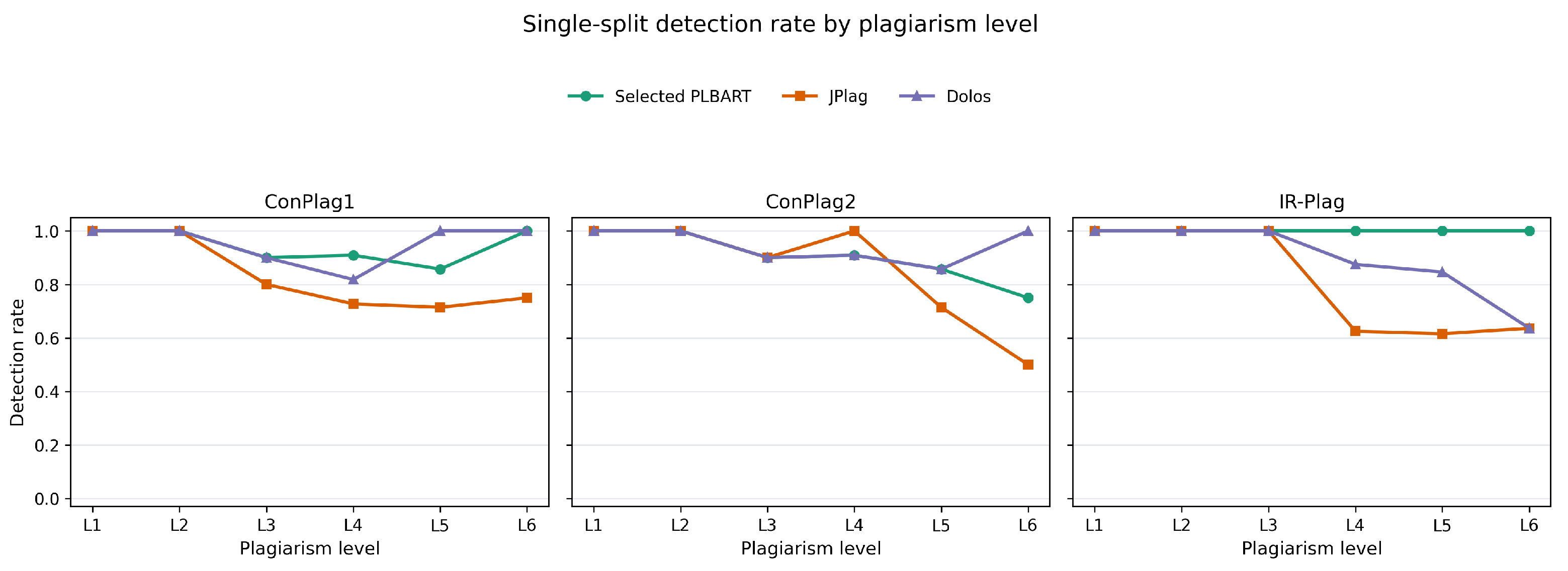
Figure 6 shows the single-split detection rate by plagiarism level for ConPlag1, ConPlag2, and IR-Plag. The rate is calculated over plagiarised pairs only. The selected PLBART follows Table 8: Pfeiffer is used for ConPlag1, while FFT is used for ConPlag2 and IR-Plag. The selected PLBART captures all L1–L2 cases in the ConPlag datasets and all levels in IR-Plag, but still misses some ConPlag L3–L6 cases. JPlag and Dolos had a lower detection rate on several harder L5–L6 levels, especially on IR-Plag.

3.2. Cross-Validation Results

A single random split can be biased, and the randomness may favour easier cases; it was used for hyperparameter selection and analysis. Therefore, we performed k-fold cross-validation to obtain a more reliable evaluation of the models and adapters. We used stratified k-fold cross-validation to preserve the original class imbalance. We selected $k=5$ to ensure sufficient test data. Using k-fold cross-validation, we split the full dataset into five folds, with four used for training and the remaining fold used for testing. This process was repeated five times, and the mean metric scores were computed. The resulting test share is larger than in the single-split case (20% rather than 15%). The results are available in

Table 9. Performance comparison ($F_1$ score ± SD) without preprocessing.

Dataset	Model	FFT	Houlsby	Pfeiffer	LoRA
ConPlag1	CodeBERT	$0.7479\pm 0.0322$	$0.6442\pm 0.1167$	$0.6395\pm 0.0554$	$0.5612\pm 0.0708$
	GraphCodeBERT	$0.6784\pm 0.0174$	$0.6127\pm 0.0467$	$0.7345\pm 0.0314$	$0.5960\pm 0.0441$
	UniXcoder	$0.7637\pm 0.0292$	$0.7123\pm 0.0312$	$0.7369\pm 0.0410$	$0.6990\pm 0.0079$
	CodeBERTa	$0.7252\pm 0.0266$	$0.7044\pm 0.0459$	$0.7110\pm 0.0439$	$0.6872\pm 0.0053$
	PLBART	$0.7907\pm 0.0177$	$0.7913\pm 0.0402$	$0.7661\pm 0.0212$	$0.7012\pm 0.0227$
	CodeT5	$0.7045\pm 0.0284$	$0.6997\pm 0.0251$	$0.6669\pm 0.0278$	$0.6872\pm 0.0408$
ConPlag2	CodeBERT	$0.6328\pm 0.0431$	$0.6512\pm 0.0434$	$0.6672\pm 0.0355$	$0.6176\pm 0.0466$
	GraphCodeBERT	$0.7038\pm 0.0364$	$0.7084\pm 0.0390$	$0.6710\pm 0.0230$	$0.6193\pm 0.0487$
	UniXcoder	$0.7823\pm 0.0404$	$0.7153\pm 0.0425$	$0.7013\pm 0.0305$	$0.6898\pm 0.0424$
	CodeBERTa	$0.7628\pm 0.0392$	$0.6897\pm 0.0220$	$0.6678\pm 0.0314$	$0.7045\pm 0.0234$
	PLBART	$0.8326\pm 0.0451$	$0.7604\pm 0.0552$	$0.8197\pm 0.0215$	$0.7635\pm 0.0241$
	CodeT5	$0.6816\pm 0.0382$	$0.7022\pm 0.0274$	$0.6742\pm 0.0313$	$0.6143\pm 0.0415$
IR-Plag	CodeBERT	$0.9837\pm 0.0156$	$0.9718\pm 0.0202$	$0.9573\pm 0.0276$	$0.9708\pm 0.0181$
	GraphCodeBERT	$0.9820\pm 0.0127$	$0.9806\pm 0.0058$	$0.9779\pm 0.0179$	$0.9794\pm 0.0109$
	UniXcoder	$0.9904\pm 0.0115$	$0.9728\pm 0.0457$	$0.9862\pm 0.0070$	$0.9809\pm 0.0156$
	CodeBERTa	$0.9750\pm 0.0164$	$0.9438\pm 0.0275$	$0.9875\pm 0.0166$	$0.9779\pm 0.0076$
	PLBART	$0.9837\pm 0.0124$	$0.9821\pm 0.0116$	$0.9877\pm 0.0089$	$0.9863\pm 0.0069$
	CodeT5	$0.9305\pm 0.0378$	$0.9012\pm 0.0131$	$0.9536\pm 0.0259$	$0.9377\pm 0.0218$
Progpedia-19	CodeBERT	$0.9139\pm 0.1143$	$0.6974\pm 0.1592$	$0.8380\pm 0.1214$	$0.7837\pm 0.1557$
	GraphCodeBERT	$0.9519\pm 0.0655$	$0.9408\pm 0.0716$	$0.9462\pm 0.0542$	$0.9711\pm 0.0294$
	UniXcoder	$0.9723\pm 0.0280$	$0.9771\pm 0.0313$	$0.9461\pm 0.0693$	$0.9417\pm 0.0670$
	CodeBERTa	$0.9669\pm 0.0367$	$0.9427\pm 0.0358$	$0.9727\pm 0.0385$	$0.9673\pm 0.0355$
	PLBART	$0.9777\pm 0.0306$	$0.9437\pm 0.0521$	$0.9395\pm 0.0841$	$0.9656\pm 0.0390$
	CodeT5	$0.9004\pm 0.0540$	$0.9270\pm 0.0118$	$0.8543\pm 0.0802$	$0.8937\pm 0.0317$

. The overall $F_1$ scores are lower than those of the single random split. Some folds were similar to the random single split, whereas other folds contained more long code pairs. A few misclassified cases in IR-Plag folds are attributed to simple Java print programs, while a few Progpedia-19 errors involve additional obfuscated code within lengthy code pairs. For the ConPlag datasets, the lower cross-validation performance relative to the random single split is linked to the distribution of longer token lengths across folds. More pairs with higher token sums were present in some test folds, and all observed ConPlag failure cases had pair context lengths greater than 512 tokens.

3.2.1. Statistical Testing

For the statistical tests, we follow the recommendations of Rainio et al. [50]. The main statistical comparison is between FFT and the best PEFT configuration for the same dataset–model pair in Table 9. This gives 24 matched observations from the four datasets and six 512-token models. Since this is a two-method paired comparison, we use a two-sided Wilcoxon signed-rank test [51] and report the paired mean difference with a 95% confidence interval. The significance level is set to $\alpha =0.05$.

We then compare the three PEFT configurations against each other using the Friedman test [52], as this comparison involves more than two matched methods. Since the Friedman test is not significant at $\alpha =0.05$, no post hoc pairwise test is required for the main interpretation.

Table 10. Main statistical testing summary for the 512-token cross-validation $F_1$ results.

Comparison	Test Result	Interpretation
FFT vs. best PEFT	Wilcoxon: $\Delta F_1=+0.0075$, 95% CI $[-0.0080,+0.0231]$, $p=0.7048$	No significant difference. The strongest adapter choice is comparable to FFT in $F_1$.
Houlsby vs. Pfeiffer vs. LoRA	Friedman: ${\chi }^2=3.25$, $p=0.1969$	No significant overall difference among the three PEFT methods; no post hoc pairwise test is required.

summarises the main statistical results. The FFT versus best-PEFT confidence interval crosses zero, which means the results do not support a consistent $F_1$ advantage for either approach when the strongest adapter is selected per dataset–model pair. The adapter-only Friedman test is also not significant, indicating no statistically significant overall difference among Houlsby, Pfeiffer, and LoRA.

3.2.2. Impact of Preprocessing and Longer Context Window

The preceding error analysis shows that several missed ConPlag cases are linked to the 512-token input limit. Surveys of long-text and long-document Transformer modelling group the main solutions into efficient attention, recurrence or memory mechanisms, sparse/global attention patterns, hierarchical modelling, compression, and segment-level aggregation [53,54,55]. Several strategies can therefore mitigate the limited-context issue in SCPD. One approach is to use models or attention mechanisms designed for longer sequences. Longformer [56], BigBird [57], and Reformer [58] reduce the cost of full self-attention and make longer context windows more practical. A second approach is to split a long program into overlapping chunks and aggregate the chunk-level predictions, although this can miss relationships between distant code regions. A third approach is hierarchical aggregation, where code fragments are encoded first and then combined at a higher level, similar to hierarchical attention models for long documents [59]. A fourth approach is to reduce or abstract the input before classification, for example by removing boilerplate or unused text, applying code normalisation [60], or summarising code with code sequence-to-sequence models [32,33]. These alternatives involve different trade-offs: long-context models increase computational cost, chunking and hierarchical aggregation require additional aggregation decisions, and input reduction may remove useful evidence.

In this paper, we focus on two practical options that can be evaluated within the same classification pipeline: preprocessing and a longer-context encoder. We studied the impact of preprocessing on both ConPlag versions, since the other two datasets were less affected by long inputs. We then evaluated a model with a longer context length.

For preprocessing, we removed comments, imports, and multiple spaces to reduce the token count, resulting in fewer misclassifications in most configurations than in the unprocessed case. The cross-validation results are shown in

Table 11. Performance comparison ($F_1$ score ± SD) with preprocessing.

Dataset	Model	FFT	Houlsby	Pfeiffer	LoRA
ConPlag1	CodeBERT	$0.7673\pm 0.0411$	$0.6950\pm 0.0275$	$0.6193\pm 0.1067$	$0.6729\pm 0.0428$
	GraphCodeBERT	$0.7706\pm 0.0486$	$0.7225\pm 0.0443$	$0.7381\pm 0.0480$	$0.6486\pm 0.0340$
	UniXcoder	$0.7982\pm 0.0188$	$0.7341\pm 0.0635$	$0.7278\pm 0.0331$	$0.7161\pm 0.0311$
	CodeBERTa	$0.7478\pm 0.0586$	$0.7143\pm 0.0437$	$0.7353\pm 0.0575$	$0.6776\pm 0.0390$
	PLBART	$0.8330\pm 0.0303$	$0.8027\pm 0.0313$	$0.8039\pm 0.0371$	$0.6979\pm 0.0264$
	CodeT5	$0.7289\pm 0.0463$	$0.6970\pm 0.0269$	$0.7122\pm 0.0442$	$0.7098\pm 0.0277$
ConPlag2	CodeBERT	$0.6558\pm 0.0373$	$0.6825\pm 0.0850$	$0.6801\pm 0.0302$	$0.6534\pm 0.0374$
	GraphCodeBERT	$0.7810\pm 0.0444$	$0.7610\pm 0.0518$	$0.6674\pm 0.0607$	$0.7421\pm 0.0338$
	UniXcoder	$0.7676\pm 0.1877$	$0.7597\pm 0.0303$	$0.7723\pm 0.0362$	$0.7229\pm 0.0385$
	CodeBERTa	$0.8218\pm 0.0256$	$0.7869\pm 0.0284$	$0.7796\pm 0.0373$	$0.7694\pm 0.0327$
	PLBART	$0.8718\pm 0.0161$	$0.8219\pm 0.0394$	$0.8456\pm 0.0505$	$0.8606\pm 0.0453$
	CodeT5	$0.7166\pm 0.0439$	$0.7193\pm 0.0421$	$0.6578\pm 0.0269$	$0.6829\pm 0.0371$

. After preprocessing, the average number of tokens decreased by approximately 3.5% in the raw dataset and by approximately 6.5% in the template-free dataset. Preprocessing improved several $F_1$ scores and assisted with the limited token length. PLBART with FFT was the best 512-token model on both ConPlag raw and template-free versions, reaching $F_1$ scores of $0.8330\pm 0.0303$ and $0.8718\pm 0.0161$, respectively.

For the longer context length, we experimented with ModernBERT [61], an enhanced BERT model with a context window of up to 8192 tokens. We used the same cross-validation setup to evaluate this model on the ConPlag datasets. We experimented with $L\in \{512,768,1024,1280\}$.

Table 12. ModernBERT $F_1$ scores by sequence length and fine-tuning method under 5-fold cross-validation: (a) without preprocessing and (b) with preprocessing.

(a) Without preprocessing
Dataset	L	FFT	Houlsby	Pfeiffer	LoRA
ConPlag1	512	$0.6616\pm 0.0505$	$0.6830\pm 0.0330$	$0.6594\pm 0.0366$	$0.6432\pm 0.0337$
	768	$0.8280\pm 0.0384$	$0.8183\pm 0.0348$	$0.8111\pm 0.0277$	$0.7188\pm 0.0121$
	1024	$0.8297\pm 0.0477$	$0.7509\pm 0.0737$	$0.8281\pm 0.0411$	$0.7717\pm 0.0449$
	1280	$0.8789\pm 0.0377$	$0.7860\pm 0.0524$	$0.8507\pm 0.0348$	$0.8177\pm 0.0572$
ConPlag2	512	$0.7871\pm 0.0431$	$0.7993\pm 0.0408$	$0.6865\pm 0.0649$	$0.6397\pm 0.0198$
	768	$0.8471\pm 0.0415$	$0.8874\pm 0.0372$	$0.8327\pm 0.0297$	$0.7782\pm 0.0475$
	1024	$0.8989\pm 0.0382$	$0.8932\pm 0.0357$	$0.8944\pm 0.0371$	$0.8520\pm 0.0371$
	1280	$0.9220\pm 0.0346$	$0.9157\pm 0.0391$	$0.8738\pm 0.0502$	$0.8549\pm 0.0350$
(b) With preprocessing
Dataset	L	FFT	Houlsby	Pfeiffer	LoRA
ConPlag1	512	$0.8066\pm 0.0261$	$0.7932\pm 0.0250$	$0.7656\pm 0.0248$	$0.6873\pm 0.0300$
	768	$0.8596\pm 0.0300$	$0.7604\pm 0.0571$	$0.8305\pm 0.0437$	$0.8070\pm 0.0407$
	1024	$0.8676\pm 0.0391$	$0.8309\pm 0.0656$	$0.8278\pm 0.0444$	$0.7765\pm 0.0411$
	1280	$0.8811\pm 0.0215$	$0.8583\pm 0.0445$	$0.8885\pm 0.0341$	$0.8731\pm 0.0354$
ConPlag2	512	$0.8338\pm 0.0348$	$0.7328\pm 0.0385$	$0.6998\pm 0.0401$	$0.7062\pm 0.0301$
	768	$0.8479\pm 0.0409$	$0.8935\pm 0.0405$	$0.8388\pm 0.1007$	$0.8253\pm 0.0577$
	1024	$0.9193\pm 0.0358$	$0.9206\pm 0.0361$	$0.9152\pm 0.0376$	$0.8653\pm 0.0369$
	1280	$0.9054\pm 0.0476$	$0.9281\pm 0.0253$	$0.8972\pm 0.0452$	$0.8916\pm 0.0266$

reports the results using $F_1$. Overall, longer context improves performance on both ConPlag datasets, and preprocessing usually improves the strongest results. Under cross-validation, the best $F_1$ scores were $0.8885\pm 0.0341$ for ConPlag1 with Pfeiffer, preprocessing, and $L=1280$, and $0.9281\pm 0.0253$ for ConPlag2 with Houlsby, preprocessing, and $L=1280$. However, ModernBERT with FFT has a larger model size of 570 MB, higher GPU usage of approximately 90%, and longer training and inference times. Comparing 512 to 1280, the training time is doubled, the inference time is increased by around 50%, and the GPU percentage is increased slightly more than double. Therefore, expanding the context length increases the cost and complexity, leading to a trade-off between $F_1$ performance and cost.

3.2.3. Comparison Against SCPDTs

The results of JPlag, Dolos, and the selected fine-tuned configurations over cross-validation are available in

Table 13. Comparison of JPlag, Dolos, and selected fine-tuned configurations across four datasets using 5-fold cross-validation. Results are reported as mean ± standard deviation.

IR-Plag
Tool/Model	P	R	${\mathbf{F}}_{\mathbf{1}}$
JPlag	$0.8036\pm 0.0154$	$0.9644\pm 0.0712$	$0.8747\pm 0.0237$
Dolos	$0.8193\pm 0.0318$	$0.9480\pm 0.0340$	$0.8785\pm 0.0265$
UniXcoder (FFT)	$0.9918\pm 0.0122$	$0.9891\pm 0.0149$	$0.9904\pm 0.0115$
UniXcoder (Pfeiffer)	$0.9919\pm 0.0074$	$0.9809\pm 0.0206$	$0.9862\pm 0.0070$
ConPlag1 (Raw)
Tool/Model	P	R	${\mathbf{F}}_{\mathbf{1}}$
JPlag	$0.8018\pm 0.0419$	$0.6950\pm 0.0798$	$0.7408\pm 0.0450$
Dolos	$0.7311\pm 0.0733$	$0.6060\pm 0.0774$	$0.6552\pm 0.0328$
PLBART (FFT)	$0.8473\pm 0.0300$	$0.8202\pm 0.0451$	$0.8330\pm 0.0303$
PLBART (Pfeiffer)	$0.8127\pm 0.0912$	$0.8008\pm 0.0217$	$0.8039\pm 0.0371$
ModernBERT (Pfeiffer, pre., $L=1280$)	$0.9071\pm 0.0394$	$0.8713\pm 0.0372$	$0.8885\pm 0.0341$
ConPlag2 (Template-Free)
Tool/Model	P	R	${\mathbf{F}}_{\mathbf{1}}$
JPlag	$0.8428\pm 0.0172$	$0.7070\pm 0.0755$	$0.7664\pm 0.0436$
Dolos	$0.7972\pm 0.0452$	$0.7072\pm 0.0748$	$0.7448\pm 0.0241$
PLBART (FFT)	$0.8992\pm 0.0460$	$0.8477\pm 0.0214$	$0.8718\pm 0.0161$
PLBART (Pfeiffer)	$0.8478\pm 0.0582$	$0.8437\pm 0.0442$	$0.8456\pm 0.0505$
ModernBERT (Houlsby, pre., $L=1280$)	$0.9174\pm 0.0240$	$0.9414\pm 0.0572$	$0.9281\pm 0.0253$
Progpedia-19
Tool/Model	P	R	${\mathbf{F}}_{\mathbf{1}}$
JPlag	$0.9800\pm 0.0400$	$0.9561\pm 0.0414$	$0.9666\pm 0.0210$
Dolos	$0.9531\pm 0.0705$	$0.9561\pm 0.0414$	$0.9517\pm 0.0286$
PLBART (FFT)	$0.9800\pm 0.0447$	$0.9778\pm 0.0497$	$0.9777\pm 0.0306$
PLBART (Pfeiffer)	$0.8948\pm 0.1402$	$1.0000\pm 0.0000$	$0.9395\pm 0.0841$

. ModernBERT is reported for the ConPlag datasets because it exceeds the best 512-token PLBART result there. UniXcoder is reported for IR-Plag because it is the strongest retained cross-validation for that dataset, while PLBART remains the strongest retained fine-tuned for Progpedia-19. For JPlag and Dolos, the parameter and threshold search is repeated using only the training data inside each fold; the remaining fold is used only for testing. Cross-validation gives a more precise and less split-dependent comparison than the single random split. JPlag and Dolos generally achieve high recall but lower precision on the ConPlag datasets, while the fine-tuned supervised models are more balanced when labelled training pairs are available. On Progpedia-19, PLBART is slightly above both tools, nearing perfect accuracy, as the dataset has easier code obfuscations.

Cross-Validation Plagiarism-Level Detection

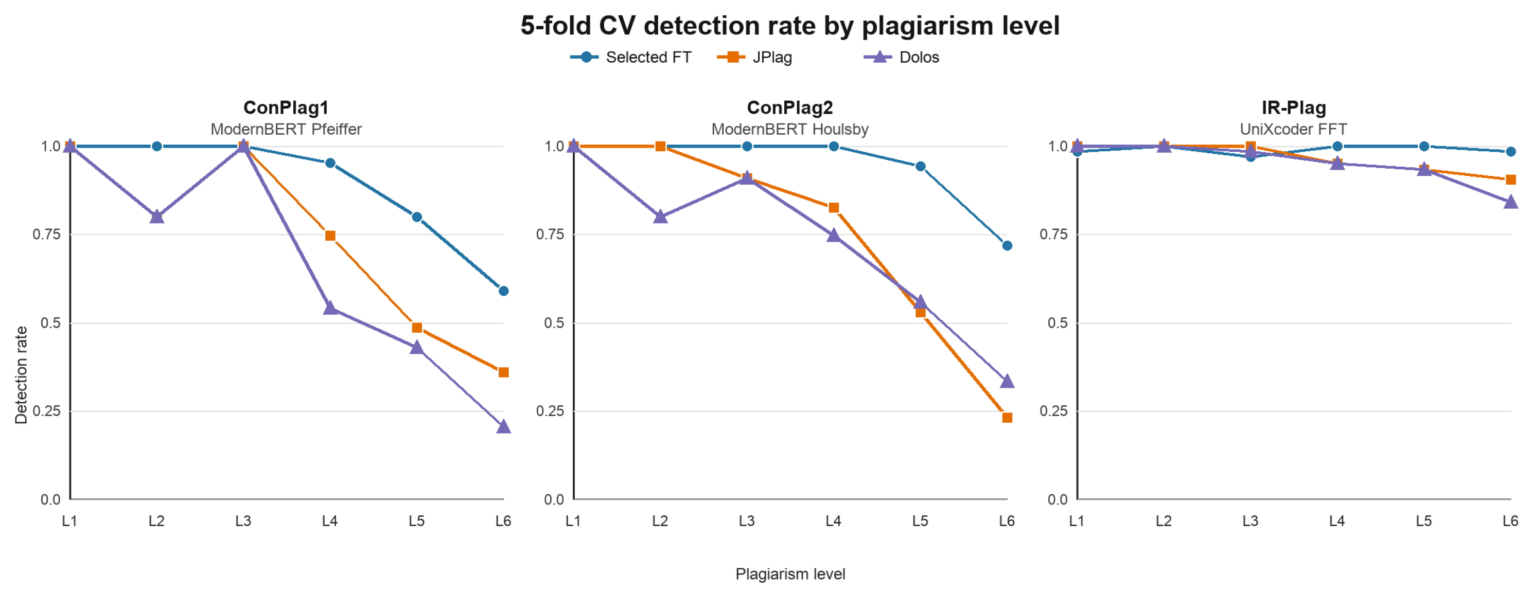
Figure 7 shows the 5-fold CV detection rate by plagiarism level for the datasets with L1–L6 annotations. The rate is calculated over plagiarised pairs only. The best fine-tuned configurations are presented in Table 13: ModernBERT is used for ConPlag1 and ConPlag2, while UniXcoder is used for IR-Plag. The pattern is clear in ConPlag1 and ConPlag2, where the best fine-tuned model keeps higher detection on the more difficult L4–L6 transformations in most cases. In IR-Plag, all methods capture L1–L4 well, while the best fine-tuned methods remain strongest on L5–L6.

4. Discussion

This section provides answers to the RQs, gives practical recommendations, discusses the empirical study threats to validity, and mentions takeaways, limitations and ideas for future work.

4.1. Answers to the Research Questions

Based on multiple experiments, we obtain the following answers to the research questions.

RQ1

How does fine-tuning the PCMs perform on the task of SCPC?

The random single split is useful for model selection and diagnostic analysis, but the main conclusion is based on 5-fold cross-validation. Under cross-validation, the selected best fine-tuned configurations achieved a higher $F_1$ than JPlag and Dolos across all datasets when labelled training data were available. The main limitation of the 512-token PCMs is the restricted context window; ModernBERT, with a longer context window and preprocessing, improved the ConPlag results.

RQ2

What is the impact of merging the adapters on PCMs for the SCPC task?

Adapters with the PCMs had similar $F_1$ performance with several models. The exceptions were CodeBERT in IR-Plag and ConPlag datasets and UniXcoder in ConPlag datasets, which led to lower performance with PEFT. The statistical analysis in Section 3.2.1 indicated no significant difference between FFT and the best PEFT configuration when each dataset–model pair was compared with its strongest adapter result.

RQ3

How do Parameter-Efficient Fine-Tuning and Full Fine-Tuning compare in terms of training time, inference time, number of trained parameters, and GPU usage?

FFT required the longest training time within the same number of epochs, while the Pfeiffer adapter required the least training time. However, adapters may require more training epochs. Adapters introduced additional inference latency relative to FFT, except for LoRA, which had the lowest inference overhead. Maximum GPU usage occurred with FFT. Full Fine-Tuning adjusts all the weights of the pre-trained model, whereas the adapters adjust around only 0.7% to 2.5% of the trainable parameters. The adapter size is added to the model size for a single-task setting. However, when multiple pre-trained models are fine-tuned on several datasets, adapters can be advantageous in terms of storage.

4.2. Practical Recommendations

The results suggest that the choice between FFT and PEFT should depend on both the data and the resources. Relevant factors include the classification accuracy ($F_1$ score), expected input length, available GPU resources, storage budget, tolerance for inference latency, and the need to maintain multiple task-specific models.

When the priority is to maximise classification performance on one dataset, and sufficient GPU resources are available, FFT remains a strong option. For long assignments, preprocessing or a longer-context model should be considered, since some missed cases were linked to the 512-token limit.

When models need to be adapted incrementally, reused across multiple tasks, or maintained in several variations, PEFT is more practical. A single base model can be shared, while small task-specific adapters are stored separately. This makes it easier to maintain different versions for assignments, courses, programming languages, or academic years without storing a full fine-tuned checkpoint for each case. The bottleneck adapters have a slight increase in inference latency, which may be tolerable in offline settings.

In practice, the best 512-token model is a reasonable starting point for short assignments with labelled historical data. If many submissions exceed the context limit, preprocessing should be applied first, followed by a longer-context model if resources allow. Overall, PEFT is better suited to institutions with limited computation capacity or many assignment-specific models, whereas FFT remains suitable when the strongest single-task performance is required, and the training cost is acceptable.

4.3. Empirical Study Threats to Validity

This section discusses the internal and external threats to the validity of this study.

4.3.1. Internal

This empirical study faces several internal validity threats. The first is that default parameters for the adapters were employed during the experiment, and altering these parameters could produce different results. Future research should focus on optimising hyperparameters for each model and adapter individually, including adapter reduction factors, LoRA ranks and scaling factors, dropout, and batch size, and monitor the impact of these parameters on the performance. The second threat is that some random single-split test partitions are small, especially IR-Plag with 69 test instances and the ConPlag versions with 137 test instances. Small test sets increase the variance of a single-split estimate, so the main conclusions are based on stratified 5-fold cross-validation rather than only the random split. The third threat is related to the use of Java-only, single-file code pair datasets. Java was selected because the available labelled SCPD datasets used in this study are Java-based and because Java is widely used in programming assignments. However, the models were not tested on other programming languages; therefore, the reported findings should not be interpreted as language-independent evidence. Cross-language validation on other languages, such as Python (3.14.5), C/C++, and JavaScript, including experiments with multilingual code models and language-specific adapters, is an important direction for future work.

4.3.2. External

External validity threats also exist in this study. The datasets, containing Java code pairs, were utilised based on the authors’ recommendations without consideration of potential annotation issues. In some cases, annotating plagiarism can be subjective and may vary from one instructor to another, even with specifying the appropriate plagiarism level. The IR-Plag repository notes (accessed on 8 July 2026) at https://github.com/oscarkarnalim/sourcecodeplagiarismdataset#important-remarks include important remarks on potential similarity among some non-plagiarised submissions and possible exclusion of one submission when using the dataset. The ConPlag L1–L6 level annotations used in this study were produced by the first author as a single annotator. Furthermore, the study relies on several Python libraries, and the results are influenced by the specific GPU used and the versions of these libraries. The datasets are small and limited to Java; hence, the generalisability of the findings should be assessed on additional datasets and programming languages in the future.

Additionally, the study used the small version of the CodeT5 model due to GPU limitations, while multiple variations of this model exist. Employing larger models could yield different results but would incur higher GPU resource costs.

4.4. Key Takeaways

This empirical study has provided several valuable insights into the use of PCMs for SCPD. Below are the key takeaways that can inform future research and practical applications.

1.

The PCMs demonstrate robustness when provided with high-quality training data. PLBART achieved the highest $F_1$ performance among the selected 512-token models, possibly due to its denoising pre-training objective on unlabelled data. By learning to recover original code from corrupted input, the model is better equipped to detect obfuscated or altered plagiarised code. This also makes it well-suited for style-based analysis tasks.

2.

When working with multiple datasets, adapters offer an efficient and modular solution. They enable easy training, merging, and toggling (ON/OFF), thereby increasing flexibility across tasks and datasets.

3.

Smaller models in the study (CodeBERTa and CodeT5 small) benefited more from PEFT. This can be attributed to the model having even fewer trainable parameters, making it more manageable and effective for learning.

4.

Due to their limited token length, the selected PCMs may fail to detect plagiarism when irrelevant or obfuscated code is inserted at the beginning, or when plagiarised content is placed toward the end of longer code files. This was verified using a model with a longer context window, but it still exhibits issues with a high combined token count across pairs. We verified this using ModernBERT with different context lengths.

5.

In real academic settings, synthetic plagiarism cases and data augmentation can help when labelled cases are scarce. Such cases can be created manually from instructor reference solutions or with automated plagiarism generation tools such as [62] or [60].

6.

Instructors may occasionally reuse programming assignments across semesters or terms [63]; while reusing assignments is not recommended, anonymised historical submissions can improve the predictive performance of plagiarism detection models when handled responsibly. Adapters may be suitable for this context because they support continual fine-tuning while retaining knowledge of previous adapters.

4.5. Limitations and Directions of Future Work

There are several limitations associated with fine-tuning PCMs for code plagiarism classification. Firstly, they require training data and perform best when the testing data are similar to the training data. Secondly, the maximum length of the small PCMs is frequently 512 tokens. Therefore, plagiarism in lengthy code is harder to detect. Thirdly, the empirical evaluation is limited to Java datasets and uses contest-based or curated benchmark data, which constrains claims about generalisation to real academic settings. Based on the findings and limitations of the paper, several future research directions could help advance research on SCPD.

1.

The maximum length of selected PCMs is 512 tokens. Therefore, plagiarism in lengthy code is harder to detect. As discussed in Section 3.2.2, possible solutions include longer-context models, sparse-attention architectures, chunking with aggregation, hierarchical aggregation, preprocessing, code normalisation, and code summarisation. In this study, we focused on preprocessing and ModernBERT as a longer-context encoder. However, this comes at the cost of greater complexity and increased resource requirements. For practitioners, preprocessing and long-context encoders are the simplest first options when assignments regularly exceed 512 tokens, whereas chunking or hierarchical aggregation may be more suitable when the complete file must be inspected. Future work should compare multiple long-context models and chunk-based strategies rather than relying on a single long-context model.

2.

This work did not cover Code Large Language Models (CodeLLMs) in the evaluation of the models. This is a limitation because CodeLLMs can be beneficial in plagiarism detection [64]. They can be used for dataset creation or annotation, for zero-shot or few-shot pair classification, or fine-tuned with PEFT or instructed to act as plagiarism detectors. They were not included in the empirical evaluation because they require a different prompting-based inference protocol, substantially larger computational resources for fine-tuning, and additional experimental choices such as prompt design, context construction, calibration, and output parsing. Future work should include a dedicated CodeLLM study, starting with zero-shot and few-shot prompting on a representative subset, followed by PEFT-based adaptation and Retrieval-Augmented Generation (RAG) when sufficient compute is available.

3.

Another evaluation approach for PCMs and CodeLLMs is to use a few instances per plagiarism level and formulate the task as few-shot pair classification, as this is more applicable in real-world scenarios.

4.

The ConPlag datasets used in this study are contest-based rather than complete real course cohorts. Contest submissions often involve single-file solutions to certain problems solved individually and may not reflect assignment code transformations. Academic plagiarism may contain partial submissions, multi-file projects, and collaboration patterns. However, they can be used as simulations of plagiarism as recommended by the dataset authors.

5.

Future work should evaluate the same SCPD pipeline on non-Java and multilingual datasets, including Python, C/C++, and JavaScript assignments. Such experiments would clarify whether the observed behaviour of FFT and PEFT transfers to languages with different syntax, typing discipline, idioms, libraries, and common obfuscation strategies. Multilingual code models and language-specific or language-adaptive adapters are promising directions for this validation.

6.

Further empirical studies could explore a broader range of models, additional adapter types, and more extensive hyperparameter optimisation. For example, several variants of LoRA have been proposed, some of which may yield improved performance [65]. Future sensitivity analysis should include adapter reduction factors, LoRA rank and scaling, dropout, batch size, and validation criteria for each model and dataset.

7.

Due to the lack of labelled training data, another way to approach the task is through semi-supervised learning, where both labelled and unlabelled data can be used to enhance the learning in the models.

5. Related Work

This section reviews related work on using pre-trained models for SCPD and the application of adapters in SE.

5.1. PCMs in SCPD

PCMs have not been extensively utilised in SCPD. Only a small number of studies have employed code models for this task. The first study by Ebrahim and Joy [66] extracted embeddings from several PCMs and computed cosine similarity between these embeddings. Multiple cosine similarity scores served as features. Subsequently, automated machine learning (AutoML) [67] was used to identify the optimal classifier given these features. Experiments were conducted on the SOurce COde reuse (SOCO) dataset [68] across Java and C/C++.

Another study by Ebrahim and Joy [69] used semantic similarity search with embeddings generated by code models to identify closely related pairs within the same SOCO dataset. Embedding models were trained both in a supervised and in an unsupervised manner. This approach aligns with IR principles.

These studies primarily relied on embeddings extracted from pre-trained models, demonstrating their potential for plagiarism detection. In contrast, this research focuses on fine-tuning the PCMs for classifying source code plagiarism instances, which, to our knowledge, has not been comprehensively achieved before.

5.2. Adapters in Software Engineering

Several related works use adapters in software engineering tasks. These studies suggest that PEFT can outperform FFT on certain code-understanding or code-generation tasks. Table 14 summarises adapter integration within SE applications, comparing tasks, pre-trained models, and PEFT methods across various SE studies. Liu et al. [70] performed an empirical study of applying several PEFT techniques on several tasks and models. The models investigated were CodeBERT, GraphCodeBERT, CodeT5, and PLBART. The adapters selected were Prefix Tuning [71], sequential adapters, IA3 [72], LoRA, parallel adapters, and mix-and-match (MAM) adapters [73]. The tasks they investigated were code summarisation, defect detection, clone detection, and code translation. They found that adapters were efficient and provided better performance in cross-language scenarios. Furthermore, the adapters achieved accuracy comparable to FFT across multiple tasks. Zou et al. [74] used the models CodeBERT, RoBERTa, CodeT5, T5, UniXcoder, and BART. The tasks were clone detection, defect detection, code search, and code translation. They experimented with the adapters of Houlsby, LoRA, Prefix, and parallel adapters. Their findings indicated that parallel adapters achieved higher accuracy than other adapter types. Additionally, they found that parallel adapters outperformed FFT on two tasks (code search and code translation). Another study by Saberi et al. [75] demonstrated that adapters performed better in low-resource code summarisation than FFT. They used the code models of CodeBERT and GraphCodeBERT and created an adapter fusion similar to MAD-X [40], which combines multiple adapters. The adapters achieved accuracy comparable to that of FFT in high-resource settings. Code Change was the focus of Liu et al. [76], which used the models CodeBERT, GraphCodeBERT, PLBART, UniXcoder and CodeT5 with sequential adapters and LoRA. The study concluded that adapters and LoRA outperformed FFT on cross-lingual and low-resource tasks. In [77], Abu Taleb et al. focused on the task of defect prediction. They fine-tuned the models CodeBERT, JavaBERT [78], CodeT5+ [79], and CodeReviewer [80] with LoRA, and these exceeded their baselines. Another task in the literature is data race detection [81], where Shen et al. used GraphCodeBERT and UniXcoder with sequential bottleneck adapters, along with Neural Architecture Search (NAS). They found that UniXcoder with NAS exceeded their other baselines.

Other related work used the emerging CodeLLMs for several tasks. For instance, Weyssow et al. [82] addressed the task of code generation. They used Large Language Models (LLMs) such as CodeGen [83] and CodeLlama [84], along with several adapters (LoRA, Prefix, Prompt [85], and IA3). Another study by Lu et al. experimented with the task of Code Review [86]. They fine-tuned LLaMA [87] with LoRA and Prefix tuning, and then compared the newly developed (LLaMA-Reviewer) with CodeT5, CodeReviewer and CommentFinder [88]. Li et al. focused on a different task, program repair [89], in which CodeLlama and DeepSeek-CodeLlama [90] were used as part of their study with several adapters (LoRA, Prompt, Prefix, IA3). Another study on the program repair task was reported in [91], where Dehghan et al. experimented with the LLMs StarCoder2 [92] and Granite [93] using LoRA adapters. Another work focused on the task of code smell detection [94], where Zhang et al. used a combination of small PCMs (CodeBERT, GraphCodeBERT, UniXcoder and CodeT5) and CodeLLMs (DeepSeek-Coder, StarCoder and CodeLlama) with four PEFT techniques (Prompt, Prefix, LoRA and IA3). They concluded that PEFT exceeded FFT in terms of accuracy in all small PCMs except CodeT5. Another SE task focused on PEFT and FFT is automatic code repair [95]. Huang et al. used the models InCoder [96], CodeGen, StarCoder and CodeLlama. They used the adapters LoRA, IA3 and AdaLoRA [97]. They concluded that LoRA outperformed FFT on the task but required slower training. Another work focused on the code summarisation task [98] using the models CodeLlama, DeepSeek-Coder, and Phi-3-mini [99], but only with a single adapter, QLoRA [100]. Afrin et al. concluded that QLoRA exceeded FFT on DeepSeek-Coder and Phi-3-mini.

Haque et al. [101] conducted a systematic literature review of PEFT methods in SE tasks, including CodeLLMs and small code models. In this work, we focused on the smaller encoder and encoder/decoder models. CodeLLMs are out of the scope of this research paper for several reasons. Firstly, we aimed to study the impact of the FFT of the models, then compared it with PEFT. FFT of LLMs is a resource-intensive task which requires more powerful GPUs. Secondly, we compared models that fall within the same range of trainable parameters (<150 M), whereas CodeLLMs, such as CodeLlama, require at least 7B parameters to fine-tune, which is not feasible under the available resource constraints. Thirdly, current Large Language Models (LLMs) rely on prompting for text classification. There are various prompting strategies, each of which requires extensive experimentation and analysis. The selected small models rely on contextual understanding provided by their encoder architecture rather than on prompting. Future work could explore the effectiveness of PEFT and prompting strategies on CodeLLMs. They are out of scope due to disparate parameter scales, limited GPU resources, and heterogeneous inference methods, including prompting.

Table 14. Related work on Parameter-Efficient Fine-Tuning for software engineering tasks in terms of tasks, explored models, and adapters.

Ref.	Task	Models	Adapters
[70]	Summarisation, defect prediction, translation, clone detection	CodeBERT, GraphCodeBERT, CodeT5, PLBART	Prefix, adapter, IA3, parallel, LoRA, MAM
[74]	Clone detection, defect detection, code search, code translation	CodeBERT, RoBERTa, CodeT5, T5, UniXcoder, BART	Houlsby, prefix, LoRA, parallel
[75]	Code summarisation, clone detection	CodeBERT, GraphCodeBERT	Adapters
[76]	Code change	CodeBERT, GraphCodeBERT, PLBART, UniXcoder, CodeT5	LoRA, adapters
[77]	Defect prediction	CodeBERT, JavaBERT, CodeT5+, CodeReviewer	LoRA
[81]	Data race detection	GraphCodeBERT, UniXcoder	Adapters
[82]	Code generation	CodeT5+, CodeGen, CodeGen2, CodeLlama	LoRA, prompt, prefix, IA3
[86]	Code review	LLaMAReviewer (LLaMA-based)	Prefix, LoRA
[89]	Program repair	CodeLlama, DeepSeek-CoderLlama	LoRA, IA3, prompt, prefix
[91]	Program repair	StarCoder2, Granite	LoRA
[94]	Code smell detection	CodeBERT, GraphCodeBERT, CodeT5, UniXcoder, DeepSeek-Coder, StarCoder, CodeLlama	Prompt, prefix, LoRA, IA3
[95]	Automatic code repair	InCoder, CodeGen, StarCoder, CodeLlama	LoRA, AdaLoRA, IA3
[98]	Code summarisation	CodeLlama, DeepSeek-Coder, Phi-3-mini	QLoRA
This Work	SCPC	CodeBERT, GraphCodeBERT, UniXcoder, CodeT5, CodeBERTa, PLBART	Adapters, LoRA

Table 14. Related work on Parameter-Efficient Fine-Tuning for software engineering tasks in terms of tasks, explored models, and adapters.

Ref.	Task	Models	Adapters
[70]	Summarisation, defect prediction, translation, clone detection	CodeBERT, GraphCodeBERT, CodeT5, PLBART	Prefix, adapter, IA3, parallel, LoRA, MAM
[74]	Clone detection, defect detection, code search, code translation	CodeBERT, RoBERTa, CodeT5, T5, UniXcoder, BART	Houlsby, prefix, LoRA, parallel
[75]	Code summarisation, clone detection	CodeBERT, GraphCodeBERT	Adapters
[76]	Code change	CodeBERT, GraphCodeBERT, PLBART, UniXcoder, CodeT5	LoRA, adapters
[77]	Defect prediction	CodeBERT, JavaBERT, CodeT5+, CodeReviewer	LoRA
[81]	Data race detection	GraphCodeBERT, UniXcoder	Adapters
[82]	Code generation	CodeT5+, CodeGen, CodeGen2, CodeLlama	LoRA, prompt, prefix, IA3
[86]	Code review	LLaMAReviewer (LLaMA-based)	Prefix, LoRA
[89]	Program repair	CodeLlama, DeepSeek-CoderLlama	LoRA, IA3, prompt, prefix
[91]	Program repair	StarCoder2, Granite	LoRA
[94]	Code smell detection	CodeBERT, GraphCodeBERT, CodeT5, UniXcoder, DeepSeek-Coder, StarCoder, CodeLlama	Prompt, prefix, LoRA, IA3
[95]	Automatic code repair	InCoder, CodeGen, StarCoder, CodeLlama	LoRA, AdaLoRA, IA3
[98]	Code summarisation	CodeLlama, DeepSeek-Coder, Phi-3-mini	QLoRA
This Work	SCPC	CodeBERT, GraphCodeBERT, UniXcoder, CodeT5, CodeBERTa, PLBART	Adapters, LoRA

This work distinguishes itself from related research by focusing on a different task: SCPD. A commonly related task in the literature is code clone detection, but the two differ in several important ways [102,103]. Firstly, code cloning typically occurs unintentionally within large codebases as developers reuse code for efficiency or consistency. In contrast, plagiarism is primarily a concern in academic settings and is committed intentionally. Secondly, students who plagiarise often attempt to obfuscate and heavily disguise the copied code to avoid detection, whereas cloning usually involves reusing slightly modified code without any attempt to hide the duplication. Thirdly, while code clones may introduce maintainability issues or vulnerabilities, they are generally tolerated in software development. However, plagiarism must not be tolerated, as it breaches academic integrity. Fourthly, the datasets employed in this study are significantly smaller (low-resource) than the benchmark code-cloning dataset BigCloneBench [104]. Krinke and Ragkhitwetsagul [105,106] investigated various issues with the labelling of the BigCloneBench dataset.

6. Conclusions

This paper presented a comprehensive empirical study evaluating the effectiveness of fine-tuned PCMs and adapter-based PEFT for low-resource SCPD. The study tested six PCMs using FFT and three adapter types: Houlsby, Pfeiffer, and LoRA.

This study found that FFT of pre-trained models demonstrated strong $F_1$ performance in classifying instances of source code plagiarism when labelled training pairs were available, and achieved higher $F_1$ scores than JPlag and Dolos in this supervised setting. Moreover, adapters had a similar performance and yielded similar results across almost all models, with a few exceptions, including CodeBERT and UniXcoder. Advantages of adapters include fewer trainable parameters and lower GPU usage, but they incur slightly higher inference time. We observed that preprocessing and using models with longer context length, like ModernBERT, helped in tackling the limited context length of the selected models and led to better classification accuracy.

This study employed an experimental setup with default adapter parameters, which is a limitation. Future work can extend these results by monitoring the effects of changing adapter hyperparameters or different adapter variations on performance. Future work should also validate the findings on non-Java and multilingual datasets. Another research direction is to explore the use of CodeLLMs for code plagiarism detection, focusing on zero-shot and few-shot prompting, prompt programming, context engineering, PEFT methods, and Retrieval-Augmented Generation (RAG).

References

1. Joy, M.; Luck, M. Plagiarism in programming assignments. IEEE Trans. Educ. 1999, 42, 129–133. [Google Scholar] [CrossRef] [Scilit]
2. Niu, C.; Li, C.; Ng, V.; Chen, D.; Ge, J.; Luo, B. An Empirical Comparison of Pre-Trained Models of Source Code. arXiv 2023, arXiv:2302.04026. [Google Scholar]
3. Pfeiffer, J.; Ruder, S.; Vulić, I.; Ponti, E.M. Modular deep learning. arXiv 2023, arXiv:2302.11529. [Google Scholar]
4. Houlsby, N.; Giurgiu, A.; Jastrzebski, S.; Morrone, B.; De Laroussilhe, Q.; Gesmundo, A.; Attariyan, M.; Gelly, S. Parameter-efficient transfer learning for NLP. In Proceedings of the International Conference on Machine Learning, PMLR, Long Beach, CA, USA, 9–15 June 2019; pp. 2790–2799. [Google Scholar]
5. Pfeiffer, J.; Rücklé, A.; Poth, C.; Kamath, A.; Vulić, I.; Ruder, S.; Cho, K.; Gurevych, I. Adapterhub: A framework for adapting Transformers. arXiv 2020, arXiv:2007.07779. [Google Scholar]
6. Hu, E.J.; Shen, Y.; Wallis, P.; Allen-Zhu, Z.; Li, Y.; Wang, S.; Wang, L.; Chen, W. Lora: Low-rank adaptation of large language models. arXiv 2021, arXiv:2106.09685. [Google Scholar]
7. Slobodkin, E.; Sadovnikov, A. Towards a Dataset of Programming Contest Plagiarism in Java. arXiv 2023, arXiv:2303.10763. [Google Scholar]
8. Karnalim, O.; Budi, S.; Toba, H.; Joy, M. Source Code Plagiarism Detection in Academia with Information Retrieval: Dataset and the Observation. Inform. Educ. 2019, 18, 321–344. [Google Scholar] [CrossRef] [Scilit]
9. Paiva, J.C.; Leal, J.P.; Figueira, Á. PROGpedia: Collection of source-code submitted to introductory programming assignments. Data Brief 2023, 46, 108887. [Google Scholar] [CrossRef] [Scilit] [PubMed]
10. Heneka, N.R. Software Plagiarism Detection on Intermediate Representation. Bachelor’s Thesis, Karlsruhe Institute of Technology (KIT), Karlsruhe, Germany, 2023. [Google Scholar]
11. Nayak, A.; Timmapathini, H.P.; Murali, V.; Gohad, A.A. Few-shot learning approaches for classifying low resource domain specific software requirements. arXiv 2023, arXiv:2302.06951. [Google Scholar]
12. Zakeri-Nasrabadi, M.; Parsa, S.; Ramezani, M.; Roy, C.; Ekhtiarzadeh, M. A systematic literature review on source code similarity measurement and clone detection: Techniques, applications, and challenges. J. Syst. Softw. 2023, 204, 111796. [Google Scholar] [CrossRef] [Scilit]
13. Faidhi, J.A.; Robinson, S.K. An empirical approach for detecting program similarity and plagiarism within a university programming environment. Comput. Educ. 1987, 11, 11–19. [Google Scholar] [CrossRef] [Scilit]
14. Vaswani, A.; Shazeer, N.; Parmar, N.; Uszkoreit, J.; Jones, L.; Gomez, A.N.; Kaiser, Ł.; Polosukhin, I. Attention is all you need. In Proceedings of the Advances in Neural Information Processing Systems, Long Beach, CA, USA, 4–9 December 2017; pp. 5998–6008. [Google Scholar]
15. Qiu, X.; Sun, T.; Xu, Y.; Shao, Y.; Dai, N.; Huang, X. Pre-trained models for natural language processing: A survey. Sci. China Technol. Sci. 2020, 63, 1872–1897. [Google Scholar] [CrossRef] [Scilit]
16. Mars, M. From Word Embeddings to Pre-Trained Language Models: A State-of-the-Art Walkthrough. Appl. Sci. 2022, 12, 8805. [Google Scholar] [CrossRef] [Scilit]
17. Devlin, J.; Chang, M.W.; Lee, K.; Toutanova, K. BERT: Pre-training of Deep Bidirectional Transformers for Language Understanding. In Proceedings of the 2019 Conference of the North American Chapter of the Association for Computational Linguistics: Human Language Technologies, Volume 1 (Long and Short Papers), Minneapolis, Minnesota, June 2019; Association for Computational Linguistics: Kerrville, TX, USA, 2019; pp. 4171–4186. [Google Scholar] [CrossRef] [Scilit]
18. Liu, Y.; Ott, M.; Goyal, N.; Du, J.; Joshi, M.; Chen, D.; Levy, O.; Lewis, M.; Zettlemoyer, L.; Stoyanov, V. Roberta: A robustly optimized bert pretraining approach. arXiv 2019, arXiv:1907.11692. [Google Scholar]
19. Lewis, M.; Liu, Y.; Goyal, N.; Ghazvininejad, M.; Mohamed, A.; Levy, O.; Stoyanov, V.; Zettlemoyer, L. BART: Denoising Sequence-to-Sequence Pre-training for Natural Language Generation, Translation, and Comprehension. In Proceedings of the 58th Annual Meeting of the Association for Computational Linguistics, Online, July 2020; Association for Computational Linguistics: Kerrville, TX, USA, 2020; pp. 7871–7880. [Google Scholar] [CrossRef] [Scilit]
20. Raffel, C.; Shazeer, N.; Roberts, A.; Lee, K.; Narang, S.; Matena, M.; Zhou, Y.; Li, W.; Liu, P.J. Exploring the limits of transfer learning with a unified text-to-text Transformer. J. Mach. Learn. Res. 2020, 21, 5485–5551. [Google Scholar]
21. Husain, H.; Wu, H.H.; Gazit, T.; Allamanis, M.; Brockschmidt, M. Codesearchnet challenge: Evaluating the state of semantic code search. arXiv 2019, arXiv:1909.09436. [Google Scholar]
22. Xu, F.F.; Alon, U.; Neubig, G.; Hellendoorn, V.J. A systematic evaluation of large language models of code. In Proceedings of the 6th ACM SIGPLAN International Symposium on Machine Programming, San Diego, CA, USA, 13 June 2022; pp. 1–10. [Google Scholar]
23. Niu, C.; Li, C.; Luo, B.; Ng, V. Deep learning meets software engineering: A survey on pre-trained models of source code. arXiv 2022, arXiv:2205.11739. [Google Scholar]
24. Zeng, Z.; Tan, H.; Zhang, H.; Li, J.; Zhang, Y.; Zhang, L. An extensive study on pre-trained models for program understanding and generation. In Proceedings of the 31st ACM SIGSOFT International Symposium on Software Testing and Analysis, Virtual, Republic of Korea, 18–22 July 2022; pp. 39–51. [Google Scholar]
25. Wong, M.F.; Guo, S.; Hang, C.N.; Ho, S.W.; Tan, C.W. Natural Language Generation and Understanding of Big Code for AI-Assisted Programming: A Review. Entropy 2023, 25, 888. [Google Scholar] [CrossRef] [Scilit] [PubMed]
26. Niu, C.; Li, C.; Ng, V.; Luo, B. Comparing the Pretrained Models of Source Code by Re-pretraining Under a Unified Setup. IEEE Trans. Neural Netw. Learn. Syst. 2024, 35, 17768–17778. [Google Scholar] [CrossRef] [Scilit] [PubMed]
27. Raihan, N.; Newman, C.; Zampieri, M. Code LLMs: A Taxonomy-based Survey. arXiv 2024, arXiv:2412.08291. [Google Scholar]
28. Feng, Z.; Guo, D.; Tang, D.; Duan, N.; Feng, X.; Gong, M.; Shou, L.; Qin, B.; Liu, T.; Jiang, D.; et al. CodeBERT: A Pre-Trained Model for Programming and Natural Languages. In Proceedings of the Findings of the Association for Computational Linguistics: EMNLP 2020, Online, November 2020; Association for Computational Linguistics: Kerrville, TX, USA, 2020; pp. 1536–1547. [Google Scholar] [CrossRef] [Scilit]
29. Guo, D.; Ren, S.; Lu, S.; Feng, Z.; Tang, D.; Liu, S.; Zhou, L.; Duan, N.; Svyatkovskiy, A.; Fu, S.; et al. Graphcodebert: Pre-training code representations with data flow. arXiv 2020, arXiv:2009.08366. [Google Scholar]
30. Wolf, T.; Debut, L.; Sanh, V.; Chaumond, J.; Delangue, C.; Moi, A.; Cistac, P.; Rault, T.; Louf, R.; Funtowicz, M.; et al. Huggingface’s Transformers: State-of-the-art natural language processing. arXiv 2019, arXiv:1910.03771. [Google Scholar] [CrossRef] [Scilit]
31. Guo, D.; Lu, S.; Duan, N.; Wang, Y.; Zhou, M.; Yin, J. Unixcoder: Unified cross-modal pre-training for code representation. arXiv 2022, arXiv:2203.03850. [Google Scholar] [CrossRef] [Scilit]
32. Wang, Y.; Wang, W.; Joty, S.; Hoi, S.C. Codet5: Identifier-aware unified pre-trained encoder/decoder models for code understanding and generation. arXiv 2021, arXiv:2109.00859. [Google Scholar]
33. Ahmad, W.U.; Chakraborty, S.; Ray, B.; Chang, K.W. Unified pre-training for program understanding and generation. arXiv 2021, arXiv:2103.06333. [Google Scholar]
34. Fu, Z.; Yang, H.; So, A.M.C.; Lam, W.; Bing, L.; Collier, N. On the Effectiveness of Parameter-Efficient Fine-Tuning. Proc. AAAI Conf. Artif. Intell. 2023, 37, 12799–12807. [Google Scholar] [CrossRef] [Scilit]
35. Ding, N.; Qin, Y.; Yang, G.; Wei, F.; Yang, Z.; Su, Y.; Hu, S.; Chen, Y.; Chan, C.M.; Chen, W.; et al. Parameter-efficient fine-tuning of large-scale pre-trained language models. Nat. Mach. Intell. 2023, 5, 220–235. [Google Scholar] [CrossRef] [Scilit]
36. Xu, L.; Xie, H.; Qin, S.Z.J.; Tao, X.; Wang, F.L. Parameter-efficient fine-tuning methods for pretrained language models: A critical review and assessment. arXiv 2023, arXiv:2312.12148. [Google Scholar]
37. Sabry, M.; Belz, A. Peft-ref: A modular reference architecture and typology for parameter-efficient finetuning techniques. arXiv 2023, arXiv:2304.12410. [Google Scholar]
38. Lialin, V.; Deshpande, V.; Rumshisky, A. Scaling down to scale up: A guide to parameter-efficient fine-tuning. arXiv 2023, arXiv:2303.15647. [Google Scholar]
39. Han, Z.; Gao, C.; Liu, J.; Zhang, J.; Zhang, S.Q. Parameter-Efficient Fine-Tuning for Large Models: A Comprehensive Survey. arXiv 2024, arXiv:2403.14608. [Google Scholar]
40. Pfeiffer, J.; Vulić, I.; Gurevych, I.; Ruder, S. MAD-X: An Adapter-Based Framework for Multi-Task Cross-Lingual Transfer. In Proceedings of the 2020 Conference on Empirical Methods in Natural Language Processing (EMNLP), Online, November 2020; Webber, B., Cohn, T., He, Y., Liu, Y., Eds.; Association for Computational Linguistics: Kerrville, TX, USA, 2020; pp. 7654–7673. [Google Scholar] [CrossRef] [Scilit]
41. Pfeiffer, J.; Kamath, A.; Rücklé, A.; Cho, K.; Gurevych, I. AdapterFusion: Non-Destructive Task Composition for Transfer Learning. In Proceedings of the 16th Conference of the European Chapter of the Association for Computational Linguistics: Main Volume, Online, April 2021; Merlo, P., Tiedemann, J., Tsarfaty, R., Eds.; Association for Computational Linguistics: Kerrville, TX, USA, 2021; pp. 487–503. [Google Scholar] [CrossRef] [Scilit]
42. Poth, C.; Sterz, H.; Paul, I.; Purkayastha, S.; Engländer, L.; Imhof, T.; Vulić, I.; Ruder, S.; Gurevych, I.; Pfeiffer, J. Adapters: A unified library for parameter-efficient and modular transfer learning. arXiv 2023, arXiv:2311.11077. [Google Scholar]
43. Zouhar, V.; Meister, C.; Gastaldi, J.; Du, L.; Vieira, T.; Sachan, M.; Cotterell, R. A Formal Perspective on Byte-Pair Encoding. In Proceedings of the Findings of the Association for Computational Linguistics: ACL 2023, Toronto, Canada, July 2023; Rogers, A., Boyd-Graber, J., Okazaki, N., Eds.; Association for Computational Linguistics: Kerrville, TX, USA, 2023; pp. 598–614. [Google Scholar] [CrossRef] [Scilit]
44. Kudo, T.; Richardson, J. SentencePiece: A simple and language independent subword tokenizer and detokenizer for Neural Text Processing. In Proceedings of the 2018 Conference on Empirical Methods in Natural Language Processing: System Demonstrations, Brussels, Belgium, November 2018; Blanco, E., Lu, W., Eds.; Association for Computational Linguistics: Kerrville, TX, USA, 2018; pp. 66–71. [Google Scholar] [CrossRef] [Scilit]
45. Gkouti, N.; Malakasiotis, P.; Toumpis, S.; Androutsopoulos, I. Should I try multiple optimizers when fine-tuning a pre-trained Transformer for NLP tasks? Should I tune their hyperparameters? In Proceedings of the 18th Conference of the European Chapter of the Association for Computational Linguistics (Volume 1: Long Papers); Association for Computational Linguistics: Kerrville, TX, USA, 2024; pp. 2555–2574. [Google Scholar]
46. Loshchilov, I.; Hutter, F. Decoupled Weight Decay Regularization. In Proceedings of the International Conference on Learning Representations, New Orleans, LA, USA, 6–9 May 2019. [Google Scholar]
47. Joshi, A.V. Machine Learning and Artificial Intelligence; Springer: Cham, Switzerland, 2020. [Google Scholar] [CrossRef] [Scilit]
48. Prechelt, L.; Malpohl, G.; Philippsen, M. Finding plagiarisms among a set of programs with JPlag. J. Univers. Comput. Sci. 2002, 8, 1016–1038. [Google Scholar] [CrossRef]
49. Maertens, R.; Van Petegem, C.; Strijbol, N.; Baeyens, T.; Jacobs, A.C.; Dawyndt, P.; Mesuere, B. Dolos: Language-agnostic plagiarism detection in source code. J. Comput. Assist. Learn. 2022, 38, 1046–1061. [Google Scholar] [CrossRef] [Scilit]
50. Rainio, O.; Teuho, J.; Klén, R. Evaluation metrics and statistical tests for machine learning. Sci. Rep. 2024, 14, 6086. [Google Scholar] [CrossRef] [Scilit] [PubMed]
51. Wilcoxon, F. Individual comparisons by ranking methods. Biom. Bull. 1945, 1, 80–83. [Google Scholar] [CrossRef] [Scilit]
52. Friedman, M. The use of ranks to avoid the assumption of normality implicit in the analysis of variance. J. Am. Stat. Assoc. 1937, 32, 675–701. [Google Scholar] [CrossRef]
53. Dong, Z.; Tang, T.; Li, J.; Zhao, W.X. A survey on long text modeling with Transformers. arXiv 2023, arXiv:2302.14502. [Google Scholar]
54. Huang, Y.; Xu, J.; Lai, J.; Jiang, Z.; Chen, T.; Li, Z.; Yao, Y.; Ma, X.; Yang, L.; Chen, H.; et al. Advancing Transformer architecture in long-context large language models: A comprehensive survey. arXiv 2023, arXiv:2311.12351. [Google Scholar]
55. Alva Principe, R.; Chiarini, N.; Viviani, M. Long Document classification in the Transformer era: A survey on challenges, advances, and open issues. Wiley Interdiscip. Rev. Data Min. Knowl. Discov. 2025, 15, e70019. [Google Scholar] [CrossRef] [Scilit]
56. Beltagy, I.; Peters, M.E.; Cohan, A. Longformer: The long-document Transformer. arXiv 2020, arXiv:2004.05150. [Google Scholar]
57. Zaheer, M.; Guruganesh, G.; Dubey, K.A.; Ainslie, J.; Alberti, C.; Ontanon, S.; Pham, P.; Ravula, A.; Wang, Q.; Yang, L.; et al. Big Bird: Transformers for longer sequences. In Proceedings of the Advances in Neural Information Processing Systems; Curran Associates Inc.: Red Hook, NY, USA, 2020; Volume 33, pp. 17283–17297. [Google Scholar]
58. Kitaev, N.; Kaiser, L.; Levskaya, A. Reformer: The efficient Transformer. In Proceedings of the International Conference on Learning Representations, Addis Ababa, Ethiopia, 26–30 April 2020. [Google Scholar]
59. Yang, Z.; Yang, D.; Dyer, C.; He, X.; Smola, A.; Hovy, E. Hierarchical attention networks for document classification. In Proceedings of the 2016 Conference of the North American Chapter of the Association for Computational Linguistics: Human Language Technologies; Association for Computational Linguistics: Kerrville, TX, USA, 2016; pp. 1480–1489. [Google Scholar]
60. Brödel, M. Preventing Automatic Code Plagiarism Generation Through Token String Normalization. Bachelor’s Thesis, Karlsruher Institut für Technologie (KIT), Karlsruhe, Germany, 2023. [Google Scholar]
61. Warner, B.; Chaffin, A.; Clavié, B.; Weller, O.; Hallström, O.; Taghadouini, S.; Gallagher, A.; Biswas, R.; Ladhak, F.; Aarsen, T.; et al. Smarter, better, faster, longer: A modern bidirectional encoder for fast, memory efficient, and long context finetuning and inference. In Proceedings of the 63rd Annual Meeting of the Association for Computational Linguistics (Volume 1: Long Papers); Association for Computational Linguistics: Kerrville, TX, USA, 2025; pp. 2526–2547. [Google Scholar]
62. Biderman, S.; Raff, E. Fooling MOSS detection with pretrained language models. In Proceedings of the 31st ACM International Conference on Information & Knowledge Management, Atlanta, GA, USA, 17–21 October 2022; pp. 2933–2943. [Google Scholar]
63. Gehringer, E.F. Reuse of homework and test questions: When, why, and how to maintain security? In Proceedings of the 34th Annual Frontiers in Education; IEEE: New York, NY, USA, 2004; p. S1F-24. [Google Scholar]
64. Brach, W.; Koš’ál, K.; Ries, M. Can Large Language Model Detect Plagiarism in Source Code? In Proceedings of the 2024 2nd International Conference on Foundation and Large Language Models (FLLM), Dubai, United Arab Emirates, 26–29 November 2024; pp. 370–377. [Google Scholar] [CrossRef] [Scilit]
65. Mao, Y.; Ge, Y.; Fan, Y.; Xu, W.; Mi, Y.; Hu, Z.; Gao, Y. A survey on lora of large language models. Front. Comput. Sci. 2025, 19, 197605. [Google Scholar]
66. Ebrahim, F.; Joy, M. Source Code Plagiarism Detection with Pre-Trained Model Embeddings and Automated Machine Learning. In Proceedings of the 14th International Conference on Recent Advances in Natural Language Processing, Varna, Bulgaria, 4–6 September 2023; pp. 301–309. [Google Scholar] [CrossRef] [Scilit] [PubMed]
67. Hutter, F.; Kotthoff, L.; Vanschoren, J. Automated Machine Learning: Methods, Systems, Challenges; Springer Nature: Cham, Switzerland, 2019. [Google Scholar]
68. Flores, E.; Rosso, P.; Moreno, L.; Villatoro-Tello, E. On the detection of source code re-use. In Proceedings of the 6th Annual Meeting of the Forum for Information Retrieval Evaluation, Bangalore, India, 5–7 December 2014; pp. 21–30. [Google Scholar]
69. Ebrahim, F.; Joy, M. Semantic Similarity Search for Source Code Plagiarism Detection: An Exploratory Study. In Proceedings of the 2024 Innovation and Technology in Computer Science Education V. 1 (ITiCSE 2024), Milan, Italy, 8–10 July 2024; p. 7. [Google Scholar] [CrossRef] [Scilit]
70. Liu, J.; Sha, C.; Peng, X. An Empirical Study of Parameter-Efficient Fine-Tuning Methods for Pre-Trained Code Models. In Proceedings of the 2023 38th IEEE/ACM International Conference on Automated Software Engineering (ASE); IEEE: New York, NY, USA, 2023; pp. 397–408. [Google Scholar]
71. Li, X.L.; Liang, P. Prefix-tuning: Optimizing continuous prompts for generation. arXiv 2021, arXiv:2101.00190. [Google Scholar]
72. Liu, H.; Tam, D.; Muqeeth, M.; Mohta, J.; Huang, T.; Bansal, M.; Raffel, C.A. Few-shot parameter-efficient fine-tuning is better and cheaper than in-context learning. Adv. Neural Inf. Process. Syst. 2022, 35, 1950–1965. [Google Scholar] [CrossRef] [Scilit]
73. He, J.; Zhou, C.; Ma, X.; Berg-Kirkpatrick, T.; Neubig, G. Towards a unified view of parameter-efficient transfer learning. arXiv 2021, arXiv:2110.04366. [Google Scholar]
74. Zou, W.; Li, Q.; Ge, J.; Li, C.; Shen, X.; Huang, L.; Luo, B. A Comprehensive Evaluation of Parameter-Efficient Fine-Tuning on Software Engineering Tasks. arXiv 2023, arXiv:2312.15614. [Google Scholar]
75. Saberi, I.; Fard, F.; Chen, F. Multilingual Adapter-based Knowledge Aggregation on Code Summarization for Low-Resource Languages. arXiv 2023, arXiv:2307.07854. [Google Scholar]
76. Liu, S.; Keung, J.; Yang, Z.; Liu, F.; Zhou, Q.; Liao, Y. Delving into Parameter-Efficient Fine-Tuning in Code Change Learning: An Empirical Study. arXiv 2024, arXiv:2402.06247. [Google Scholar]
77. Abu Talib, M.; Bou Nassif, A.; Azzeh, M.; Alesh, Y.; Afadar, Y. Parameter-efficient fine-tuning of pre-trained code models for just-in-time defect prediction. Neural Comput. Appl. 2024, 36, 16911–16940. [Google Scholar] [CrossRef] [Scilit]
78. De Sousa, N.T.; Hasselbring, W. Javabert: Training a Transformer-based model for the java programming language. In Proceedings of the 2021 36th IEEE/ACM International Conference on Automated Software Engineering Workshops (ASEW); IEEE: New York, NY, USA, 2021; pp. 90–95. [Google Scholar]
79. Wang, Y.; Le, H.; Gotmare, A.D.; Bui, N.D.; Li, J.; Hoi, S.C. Codet5+: Open code large language models for code understanding and generation. arXiv 2023, arXiv:2305.07922. [Google Scholar]
80. Li, Z.; Lu, S.; Guo, D.; Duan, N.; Jannu, S.; Jenks, G.; Majumder, D.; Green, J.; Svyatkovskiy, A.; Fu, S.; et al. CodeReviewer: Pre-Training for Automating Code Review Activities. arXiv 2022, arXiv:2203.09095. [Google Scholar]
81. Shen, Y.; Peng, M.; Zhang, F.; Wu, Q. Data race detection via few-shot parameter-efficient fine-tuning. J. Syst. Softw. 2025, 222, 112289. [Google Scholar] [CrossRef] [Scilit]
82. Weyssow, M.; Zhou, X.; Kim, K.; Lo, D.; Sahraoui, H. Exploring parameter-efficient fine-tuning techniques for code generation with large language models. arXiv 2023, arXiv:2308.10462. [Google Scholar]
83. Nijkamp, E.; Pang, B.; Hayashi, H.; Tu, L.; Wang, H.; Zhou, Y.; Savarese, S.; Xiong, C. Codegen: An open large language model for code with multi-turn program synthesis. arXiv 2022, arXiv:2203.13474. [Google Scholar]
84. Roziere, B.; Gehring, J.; Gloeckle, F.; Sootla, S.; Gat, I.; Tan, X.E.; Adi, Y.; Liu, J.; Sauvestre, R.; Remez, T.; et al. Code llama: Open foundation models for code. arXiv 2023, arXiv:2308.12950. [Google Scholar]
85. Lester, B.; Al-Rfou, R.; Constant, N. The power of scale for parameter-efficient prompt tuning. arXiv 2021, arXiv:2104.08691. [Google Scholar]
86. Lu, J.; Yu, L.; Li, X.; Yang, L.; Zuo, C. LLaMA-Reviewer: Advancing Code Review Automation with Large Language Models through Parameter-Efficient Fine-Tuning. In Proceedings of the 2023 IEEE 34th International Symposium on Software Reliability Engineering (ISSRE); IEEE: New York, NY, USA, 2023; pp. 647–658. [Google Scholar]
87. Touvron, H.; Lavril, T.; Izacard, G.; Martinet, X.; Lachaux, M.A.; Lacroix, T.; Rozière, B.; Goyal, N.; Hambro, E.; Azhar, F.; et al. Llama: Open and efficient foundation language models. arXiv 2023, arXiv:2302.13971. [Google Scholar]
88. Hong, Y.; Tantithamthavorn, C.; Thongtanunam, P.; Aleti, A. Commentfinder: A simpler, faster, more accurate code review comments recommendation. In Proceedings of the 30th ACM joint European Software Engineering Conference and Symposium on the Foundations of Software Engineering, Singapore, 14–18 November 2022; pp. 507–519. [Google Scholar]
89. Li, G.; Zhi, C.; Chen, J.; Han, J.; Deng, S. A Comprehensive Evaluation of Parameter-Efficient Fine-Tuning on Automated Program Repair. arXiv 2024, arXiv:2406.05639. [Google Scholar]
90. Guo, D.; Zhu, Q.; Yang, D.; Xie, Z.; Dong, K.; Zhang, W.; Chen, G.; Bi, X.; Wu, Y.; Li, Y.; et al. DeepSeek-Coder: When the Large Language Model Meets Programming–The Rise of Code Intelligence. arXiv 2024, arXiv:2401.14196. [Google Scholar]
91. Dehghan, M.; Wu, J.J.; Fard, F.H.; Ouni, A. MergeRepair: An Exploratory Study on Merging Task-Specific Adapters in Code LLMs for Automated Program Repair. arXiv 2024, arXiv:2408.09568. [Google Scholar]
92. Lozhkov, A.; Li, R.; Allal, L.B.; Cassano, F.; Lamy-Poirier, J.; Tazi, N.; Tang, A.; Pykhtar, D.; Liu, J.; Wei, Y.; et al. Starcoder 2 and the stack v2: The next generation. arXiv 2024, arXiv:2402.19173. [Google Scholar]
93. Mishra, M.; Stallone, M.; Zhang, G.; Shen, Y.; Prasad, A.; Soria, A.M.; Merler, M.; Selvam, P.; Surendran, S.; Singh, S.; et al. Granite code models: A family of open foundation models for code intelligence. arXiv 2024, arXiv:2405.04324. [Google Scholar]
94. Zhang, B.; Liang, P.; Zhou, X.; Zhou, X.; Lo, D.; Feng, Q.; Li, Z.; Li, L. A Comprehensive Evaluation of Parameter-Efficient Fine-Tuning on Method-Level Code Smell Detection. arXiv 2024, arXiv:2412.13801. [Google Scholar]
95. Huang, K.; Zhang, J.; Bao, X.; Wang, X.; Liu, Y. Comprehensive Fine-Tuning Large Language Models of Code for Automated Program Repair. IEEE Trans. Softw. Eng. 2025, 51, 904–928. [Google Scholar] [CrossRef] [Scilit]
96. Fried, D.; Aghajanyan, A.; Lin, J.; Wang, S.; Wallace, E.; Shi, F.; Zhong, R.; Yih, W.t.; Zettlemoyer, L.; Lewis, M. Incoder: A generative model for code infilling and synthesis. arXiv 2022, arXiv:2204.05999. [Google Scholar]
97. Zhang, Q.; Chen, M.; Bukharin, A.; Karampatziakis, N.; He, P.; Cheng, Y.; Chen, W.; Zhao, T. Adalora: Adaptive budget allocation for parameter-efficient fine-tuning. arXiv 2023, arXiv:2303.10512. [Google Scholar]
98. Afrin, S.; Call, J.; Nguyen, K.N.; Chaparro, O.; Mastropaolo, A. Resource-Efficient & Effective Code Summarization. arXiv 2025, arXiv:2502.03617. [Google Scholar]
99. Abdin, M.; Aneja, J.; Awadalla, H.; Awadallah, A.; Awan, A.A.; Bach, N.; Bahree, A.; Bakhtiari, A.; Bao, J.; Behl, H.; et al. Phi-3 technical report: A highly capable language model locally on your phone. arXiv 2024, arXiv:2404.14219. [Google Scholar]
100. Dettmers, T.; Pagnoni, A.; Holtzman, A.; Zettlemoyer, L. Qlora: Efficient finetuning of quantized llms. Adv. Neural Inf. Process. Syst. 2023, 36, 10088–10115. [Google Scholar] [CrossRef] [Scilit]
101. Haque, M.Z.; Afrin, S.; Mastropaolo, A. A Systematic Literature Review of Parameter-Efficient Fine-Tuning for Large Code Models. arXiv 2025, arXiv:2504.21569. [Google Scholar]
102. Sağlam, T. Mitigating Automated Obfuscation Attacks on Software Plagiarism Detection Systems. Ph.D. Thesis, Karlsruher Institut für Technologie (KIT), Karlsruhe, Germany, 2025. [Google Scholar] [CrossRef]
103. Mariani, L.; Micucci, D. AuDeNTES: Automatic Detection of teNtative plagiarism according to a rEference Solution. ACM Trans. Comput. Educ. 2012, 12, 1–26. [Google Scholar] [CrossRef] [Scilit]
104. Svajlenko, J.; Islam, J.F.; Keivanloo, I.; Roy, C.K.; Mia, M.M. Towards a big data curated benchmark of inter-project code clones. In Proceedings of the 2014 IEEE International Conference on Software Maintenance and Evolution; IEEE: New York, NY, USA, 2014; pp. 476–480. [Google Scholar]
105. Krinke, J.; Ragkhitwetsagul, C. Bigclonebench considered harmful for machine learning. In Proceedings of the 2022 IEEE 16th International Workshop on Software Clones (IWSC); IEEE: New York, NY, USA, 2022; pp. 1–7. [Google Scholar]
106. Krinke, J.; Ragkhitwetsagul, C. How the Misuse of a Dataset Harmed Semantic Clone Detection. arXiv 2025, arXiv:2505.04311. [Google Scholar]
107. Mersha, M.; Lam, K.; Wood, J.; AlShami, A.; Kalita, J. Explainable artificial intelligence: A survey of needs, techniques, applications, and future direction. Neurocomputing 2024, 599, 128111. [Google Scholar] [CrossRef] [Scilit]
108. Cao, S.; Sun, X.; Widyasari, R.; Lo, D.; Wu, X.; Bo, L.; Zhang, J.; Li, B.; Liu, W.; Wu, D.; et al. A systematic literature review on explainability for machine/deep learning-based software engineering research. arXiv 2024, arXiv:2401.14617. [Google Scholar]
109. Lundberg, S.M.; Lee, S.I. A Unified Approach to Interpreting Model Predictions. In Advances in Neural Information Processing Systems 30; Guyon, I., Luxburg, U.V., Bengio, S., Wallach, H., Fergus, R., Vishwanathan, S., Garnett, R., Eds.; Curran Associates, Inc.: Red Hook, NY, USA, 2017; pp. 4765–4774. [Google Scholar]
Figure 1. Methodology to answer RQ1.
Applsci 16 07156 g001
Figure 2. Methodology to answer RQ2.
Applsci 16 07156 g002
Figure 3. A single Transformer block architecture, adapters, and adapter block [4,14,40,41]. (a) Transformer encoder architecture. (b) Adapter block components. (c) Houlsby adapter. (d) Pfeiffer adapter.
Applsci 16 07156 g003
Figure 4. LoRA adapter architecture [6].
Applsci 16 07156 g004
Figure 5. ConPlag raw efficiency comparison heat maps. The colour bars show the value scale, and darker blue cells indicate larger values within each metric. (a) Training time in seconds. (b) Inference time in seconds. (c) Percentage of trainable parameters. (d) Percentage of GPU usage. (e) Model size in MB for the pre-trained models and adapters.
Applsci 16 07156 g005
Figure 6. Single-split plagiarism-level detection for the selected PLBART, JPlag, and Dolos.
Applsci 16 07156 g006
Figure 7. Five-fold cross-validation plagiarism-level detection for the best fine-tuned, JPlag, and Dolos.
Applsci 16 07156 g007