Low-Carbon Urban Freight Optimization: Per-Order Adaptive Mode Mixing with Demonstration-Regularized Constrained Reinforcement Learning

Abstract

Urban last-mile delivery is a rapidly growing source of city-centre emissions, and decarbonizing it without eroding service quality has become imperative for climate goals. Operators are turning to multimodal systems that integrate road vehicles, off-peak metro freight, and electric drones—yet the optimal delivery channel varies dynamically with location and time. Current RL-based schedulers handle constraints via manually tuned penalty weights, lacking formal safety guarantees, and the feasibility of online carbon-cap enforcement under partial observability remains an open question. To address this, we model the problem as a Constrained Markov Decision Process (CMDP) and propose a demonstration-regularized Lagrangian deep RL algorithm. Our approach learns an online policy that is model-free at deployment—it controls emissions in expectation against a hard carbon budget, makes per-order decisions using only state observations, and operates without an emission model at test time (the demonstrator used at training time does access the emissions model, so “model-free” refers strictly to the deployment phase). Experiments on synthetic benchmarks and a Nanjing-inspired scenario—grounded in real metro topology and population-weighted demand—show that our policy achieves emissions within 1.3% of the offline optimum. It robustly tracks a ±17% carbon-budget band across a threefold daily volume range and a threefold city-scale range, with zero per-instance tuning. By contrast, a standard PPO with fixed penalty weights consistently degrades to single-mode selection. Our findings suggest that hard carbon budgets can be controlled in expectation online at modest cost—a step toward operator-facing low-carbon logistics whose average emissions honour a binding carbon budget, though external validation on operational data and a risk-sensitive formulation that upgrades this average control into per-day compliance are still required before deployment.

1. Introduction

The domain of urban last-mile logistics is growing rapidly under the influence of e-commerce and on-demand retail, and its heavy reliance on diesel road vehicles makes it a disproportionate contributor to city-centre carbon emissions and traffic congestion [1]. Under China’s “dual-carbon” commitments (carbon peak by 2030 and neutrality by 2060) [2], operators face mounting pressure to cut delivery emissions while preserving service quality. Road vehicles will remain the backbone of urban delivery, but two complementary low-carbon channels are increasingly available to relieve them: off-peak metro freight, which repurposes spare underground rail capacity for trunk haulage [3], and electric last-mile drones, which bypass surface congestion on short final legs [4]. Used together, the road fleet and these channels form a multimodal delivery system whose emissions can be substantially lower than a truck-only operation, provided the operator decides well, for each order, which channel or combination of channels should carry it. It is this real-time channel-selection decision, under a binding carbon budget and customer service constraints, that we study.

However, coordinating such a delivery operation is demanding. For every incoming order, the operator must choose a delivery channel, the transfer points between metro and road vehicles and the launch and landing sites for drones, and the resulting vehicle and drone routes, all while keeping the day’s total carbon emissions, late deliveries, drone energy use, and metro-station load within firm limits. Two families of methods are commonly applied. Mathematical-programming approaches, such as mixed-integer formulations and multi-objective evolutionary or ALNS–ACO heuristics, attain near-optimal plans at the network-design scale but assume the demand is known and struggle with decisions that must be made online as orders arrive [5,6,7]. Reinforcement-learning approaches handle the online and stochastic nature of the problem naturally, but they conventionally fold every constraint into a single weighted-penalty reward ($r=-c-{\sum }_i{\alpha }_i{c}_i$) [8,9]. For an operator who must respect a firm carbon cap, this is unsatisfactory: a finite penalty can always be “paid off” by a policy that violates the cap where it is profitable to do so, so the limit holds only on average rather than reliably; the penalty weights (${\alpha }_i$) that achieve a given emissions target depend on the units and scale of cost and emissions and must be re-tuned for every city, season, or fleet, and a single scalar reward fuses the economic and environmental objectives, leaving the operator no view of how much each unit of carbon abatement actually costs.

What makes this decision genuinely hard is that the right channel is not a fixed property of a delivery; it depends on where the order is going, when it arrives, and how much of the day’s carbon budget is still available. An order bound for a district well served by metro can be carried at a very low carbon cost through a rail trunk with a short final leg, whereas the same channel is wasteful for an order near the depot, which a road vehicle can reach directly. Demand is also not known in advance: orders arrive throughout the day, the carbon already spent constrains what remains affordable, and the operator cannot re-optimize a static plan after every arrival. Therefore, a scheduler must commit to a channel for each order online, balancing immediate operating cost against the cumulative carbon and service obligations of the whole day. This is the kind of sequential decision-making under uncertainty that reinforcement learning is suited to; the difficulty is that the carbon cap and service requirements are firm operating limits rather than soft preferences, and conventional reward-shaping handles them poorly, as noted above.

We therefore take a constrained route: we cast carbon-aware multimodal dispatch as a Constrained Markov Decision Process (CMDP) [10] in which the carbon cap and service requirements are explicit constraints rather than reward terms and solve it with a Lagrangian deep reinforcement-learning algorithm that adjusts the balance between cost and carbon automatically, without the operator hand-tuning penalty weights. Once the cost–carbon trade-off varies across the city, no single channel is the right answer for every order: the policy that best meets demand within the carbon budget routes different orders through different channels. A plain constrained policy does not arrive at this behaviour on its own; we develop a demonstration-regularized training scheme that lets it do so. The numerical experiments in Section 5 demonstrate the algorithmic behaviour under stylised conditions and are a necessary but not sufficient step before operational deployment.

This study makes three contributions. First, we formulate real-time carbon-aware multimodal dispatch as a constrained Markov decision process that selects, for each incoming order, among road, metro-freight, and drone delivery channels under a daily carbon budget, customer time windows, and operational limits on drone range and metro-station capacity, with a carbon intensity that varies by time of day and city region. To the best of our knowledge, this is the first such formulation that treats all three channels, together with the carbon cap, as a hard constraint, and we release an open simulator of the setting. Second, we develop a demonstration-regularized fine-tuning recipe that lets a Lagrangian-PPO agent control expected emissions against a binding carbon budget online (i.e., the mean over evaluation days is honoured, though individual days may deviate) while choosing a delivery channel for each order based on its state (destination, time, and remaining budget); the deployed policy is model-free at deployment (it requires no emissions model at decision time, though the demonstrator does access the emissions model during training), and plain constrained RL does not reach such a state-dependent policy. Third, we provide a thorough empirical study: against a penalty-free scheduler, the method nearly eliminates carbon and time-window violations at a modest operating-cost premium on synthetic city instances, and on a Nanjing-inspired instance built from the city’s metro topology and population-weighted demand, it learns a near-feasible per-order policy markedly cheaper than any single-channel alternative; we further benchmark against an offline clairvoyant optimum computed by an exact mixed-integer solver, finding our online model-free policy to be within a small margin of the offline optimum, and we report honest ablations of each design choice.

This study tests three hypotheses. (H1) Constrained reinforcement learning can control expected daily emissions against a hard cap online, without hand-tuned reward weights. (H2) In a heterogeneous city, no single fixed channel serves demand optimally under a binding carbon cap, so the constraint-active policy is per-order rather than one-channel. (H3) Demonstration-regularized fine-tuning is a necessary training ingredient—plain Lagrangian-PPO does not discover the per-order policy on its own. Section 5 tests these hypotheses empirically.

The remainder of the study is organized as follows. Section 2 surveys related work in multimodal urban-logistics optimization, learning-based vehicle routing, and constrained reinforcement learning. Section 3 describes the delivery setting and formalizes it as a CMDP. Section 4 develops the solution method. Section 5 reports the experiments, including the main comparison, ablations, per-order channel assignment, and the Nanjing-inspired case study. Section 6 discusses when the approach is preferable and its limitations, and Section 7 concludes the paper.

2. Related Work

2.1. Multimodal Urban Logistics Optimization

The classical literature on multimodal logistics network design uses Mixed-Integer Linear Programming (MILP) augmented with multi-objective Pareto solvers. Fu et al. [5] solved a two-stage problem with NSGA-II at the strategic facility-location layer and a genetic algorithm at the routing layer; their carbon-tax internalization framework reports a 7% mileage reduction and 226.5 kg carbon savings under hub consolidation. Guo et al. [6] established a bi-level MIP under a carbon-tax constraint and demonstrated that network reconfiguration is a low-cost mitigation lever. For multi-objective routing, Yang and Jiang [7] coupled ALNS with ACO under time-varying networks; Peng et al. [11] extended this frameworkto four objectives (time, cost, carbon, and food waste) using MC-ObOEA The cold-chain literature has produced highly specialized variants [12,13,14].

The metro-freight thread is younger but growing rapidly. Hu et al. [3] proposed a hub-and-spoke metro-based underground logistics network and reported ground-side mileage reductions of 15–$20\%$ in an urban case study; Delle Donne et al. [15] formalised a broader “freight-on-transit” strategic planning problem in which parcels ride passenger transit lines. The last-mile drone literature establishes hierarchical hub designs and mixed-integer launch-pad placement models that account for range and energy limits [4,16,17], and exact branch-and-bound methods for the underlying truck–drone TSP have been developed for European operators [18]. More generally, European operations research has advanced the design of urban-logistics systems from two perspective: two-echelon last-mile models with satellite depots under the on-demand economy [19] and electric location-routing under time windows and partial recharging that addresses the fleet-electrification side of decarbonisation [20]. None of these works models all three modes (metro, ground, and drone) simultaneously under explicit constraint-satisfaction guarantees.

2.2. Deep Reinforcement Learning for Vehicle Routing

Learning-based routing began with attention-based sequence-to-sequence policies that construct vehicle-routing solutions in an end to end manner [21,22,23], and the idea has since been carried into last-mile delivery. Recent work spans single-objective policies for last-mile fleets [4], two-objective extensions for cold-chain delivery that trade cost against spoilage or energy [9], and early attempts at coordinating more than one transport mode [24,25]. Two studies are especially close to our setting: Liu et al. [9] developed a learning policy for an agricultural location-routing problem with time windows, and Cho et al. [26] scheduled joint truck–drone delivery with a criterion-based rule for the assignment of orders to a mode. In both of the abovementioned methods, however, the operating limits enter the learning objective only as soft penalty terms, so the learned policy offers no guarantee of respecting them, and neither study addresses a binding carbon budget across an interacting road, rail, and air fleet. Thus, the gap we target is twofold: the constraint, especially the carbon cap, is treated as firm rather than soft, and the three channels are coordinated jointly rather than two at a time.

2.3. Constrained Reinforcement Learning

Constrained Markov decision processes, in which a policy minimizes a cost subject to bounds on auxiliary cost signals, were formalized by Altman [10], and a mature toolbox now exists for solving them. Constrained policy optimization takes a trust-region step bounded by a constraint-cost surrogate [27]; reward-constrained policy optimization adapts a Lagrange multiplier via gradient ascent so that the dual variable rises until the constraint is met [28]; interior-point methods replace the constraint with a logarithmic barrier [29]; and the Responsive-Safety scheme stabilizes the multiplier update with a proportional–integral controller [30]. These methods were developed and are overwhelmingly evaluated in autonomous driving, robotics, and game domains, where the “constraint” is typically a safety limit on a physical agent. Their transfer to logistics is recent and partial: a few studies have used soft Lagrangian-style penalties for emissions or service levels [6,31], but they stop short of an explicit constrained formulation. We are not aware of prior work bringing a constrained-MDP treatment, a time- and region-varying carbon model, and a like-for-like comparison against constrained-RL baselines to the joint metro–road–drone delivery problem; closing this gap and identifying what such a constrained policy must do to serve demand within a carbon budget are the aims of this study.

3. Problem Description

3.1. System Overview

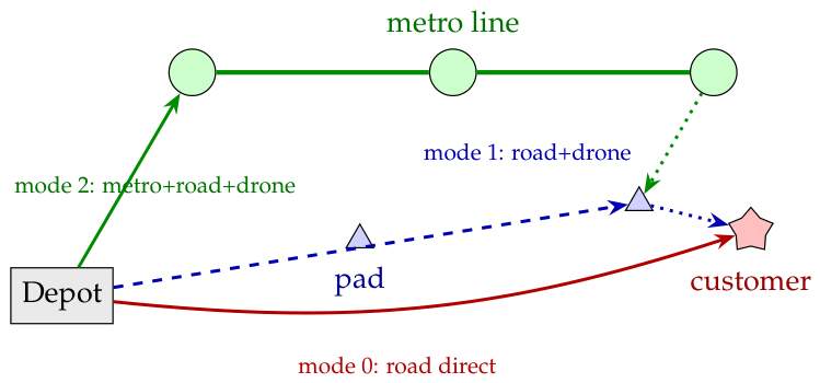
We consider a single distribution centre (depot) at ${\mathbf{x}}_0\in {\mathbb{R}}^2$, $K_M$ metro stations, $K_L$ drone landing pads, and a stochastic stream of customer orders. Each order ($o_i$) has an arrival time ($t_i^{\mathrm{arr}}$), a destination (${\mathbf{d}}_i\in {\mathbb{R}}^2$), a weight ($w_i$), and a delivery deadline ($t_i^{\mathrm{tw}}$). Three delivery modes are available:

• Mode 0 (truck-direct): A ground vehicle leaves the depot, delivers to ${\mathbf{d}}_i$, and returns.
• Mode 1 (truck+drone): A ground vehicle leaves the depot for the nearest landing pad to ${\mathbf{d}}_i$; a drone completes the pad-to-destination leg.
• Mode 2 (metro+truck+drone): The package is shipped via metro to the nearest metro station to ${\mathbf{d}}_i$; a truck moves it to the nearest landing pad; a drone completes the delivery.

Figure 1 illustrates the three channels for a single order.

These three channels are not an arbitrary design choice; they correspond to the distinct delivery needs that arise across a city and to options operators are already deploying. An order to a customer near the depot—or one with a tight deadline that cannot absorb a transfer—is best served by sending a road vehicle directly: this is the incumbent mode for most urban delivery today and remains the cheapest when distances are short. An order in a dense or congested district, where a vehicle would crawl through traffic for the final blocks but a drone can fly the last stretch directly, is better served by a road vehicle that hands the parcel to a drone at a nearby pad, a truck–drone combination already piloted at scale by major Chinese carriers [4]. An order bound for a district far from the depot but well connected by rail is best carried on the metro trunk during off-peak hours, with a road vehicle and drone completing the local leg, the emerging metro-freight pattern validated on Nanjing data [3]. Thus, the three channels span a clear progression from low overhead and high carbon to higher overhead and low carbon, and which is most appropriate is a property of the individual order rather than of the system as a whole. Within a channel, the choice of transfer station and drone pad is resolved by a nearest-neighbour rule so that the operator’s online decision reduces to the selection of the channel; joint optimization of routes, timing, and transfer points is a natural extension we leave to future work.

For each mode, the per-order cost is computed as

$$c(o_i,m)=c_T·d_T\left(m\right)+c_D·d_D\left(m\right)+c_M·d_M\left(m\right)+c_X·n_X\left(m\right),$$

where $d_T,d_D$, and $d_M$ are the truck-, drone-, and metro-leg distances under mode m (Manhattan for ground, Euclidean for drone); $c_T, c_D$, and $c_M$ are unit-cost coefficients; $c_X$ is a per-transhipment cost; and $n_X\left(m\right)\in \{0,1,2\}$ is the number of transhipments. The per-order carbon emission combines a time-of-day factor ($\alpha \left(t\right)$), a region factor ($\beta \left({\mathbf{d}}_i\right)$), and a truck-only spatial factor ($\sigma \left({\mathbf{d}}_i\right)$) that captures urban congestion in carbon-hotspot areas:

$$g(o_i,m,t)=\alpha \left(t\right)·\beta \left({\mathbf{d}}_i\right)·\left[e_T·d_T\left(m\right)·\sigma \left({\mathbf{d}}_i\right)+e_D·d_D\left(m\right)+e_M·d_M\left(m\right)\right].$$

Here $e_T,e_D$, and $e_M$ are unit-emission intensities. The $\sigma \left({\mathbf{d}}_i\right)$ factor models the empirical observation that ground-traffic congestion in dense urban areas amplifies vehicle emissions but does not affect rail or air emissions [32].

Order arrivals and the demand distribution. Orders arrive online over a $T_{max}$-minute operating day. Arrival times ($t_i^{\mathrm{arr}}$) follow a Poisson process at a rate of $\rho$ per minute., so the day produces $\sim \rho T_{max}$ orders, on average (e.g., $\rho =0.4$ and $T_{max}=480$ correspond to $\approx 192$ orders). Each order ($o_i$) also has a destination (${\mathbf{d}}_i$) drawn from a demand distribution ($\mathcal{D}$) over the city, a weight ($w_i\sim \mathrm{Unif}(w_{min},w_{max})$), and a deadline ($t_i^{\mathrm{tw}}$). Two demand distributions appear in this study: $\mathcal{D}$ is uniform over the grid by default, and on the Nanjing-inspired instance of Section 5.7, it is a population-weighted Gaussian mixture over five fixed centres (one CBD with a mass of $0.40$ and four sub-centres, each with a mass of $0.15$).

3.2. Constrained MDP Formulation

We formalize the joint scheduling problem as a Constrained Markov Decision Process (CMDP),

$${\mathcal{M}}_C=\langle \mathcal{S},\mathcal{A},\mathcal{P},c,{\left\{c_i\right\}}_{i=1}^{N_c},{\left\{b_i\right\}}_{i=1}^{N_c},\gamma \rangle ,$$

where $\mathcal{S}$ is the state space, $\mathcal{A}$ is the action space, $\mathcal{P}$ is a transition kernel, c is the scalar cost, and $\left\{c_i\right\}$ represents constraint costs, each with budget ($b_i$) and discount ($\gamma$) defined as follows.

State space ($\mathcal{S}$): The state $s_t$ at decision step t is a 17-dimensional feature vector composed of five blocks:

• Temporal block: Relative time ($t/T_{max}$) and fraction of remaining orders.
• Order block: Destination coordinates, distance to depot/nearest metro station/nearest landing pad, weight, waiting time, and time-window slack.
• Carbon block: Remaining carbon-budget fraction and current carbon factor ($\alpha \left(t\right)\beta \left(\mathbf{d}\right)$).
• Time-window block: Remaining TW budget fraction.
• Resource block: Current metro hour-bucket load fraction and cumulative cost.

The remaining-budget components are part of the state, which lets the policy see how much budget has been spent and pace the constraint accordingly.

Action space ($\mathcal{A}$): The discrete action ($a_t\in \{0,1,2\}$) assigns the next pending order to one of the three delivery modes. Conditioned on the mode, the simulator computes the deterministic kinematics that determine cost, carbon, time-window violation, and constraint violations.

Reward and constraint costs. The single-step reward and constraint costs are

$$r_t=-c(o_t,a_t),c_{i,t}=\left\{\begin{array}{cc}g(o_t,a_t,t)\hfill & i=1\left(\mathrm{carbon}\right)\hfill \\ max(0,t^{\mathrm{arr}}(o_t,a_t)-t_{o_t}^{\mathrm{tw}})\hfill & i=2(\mathrm{time}\mathrm{window})\hfill \\ max(0,d_D(o_t,a_t)-R_{max})\hfill & i=3(\mathrm{drone}\mathrm{range})\hfill \\ max(0,{\rho }_h\left(t\right)-{\rho }_{max})\hfill & i=4(\mathrm{metro}\mathrm{capacity})\hfill \end{array}\right.$$

Optimization problem. The policy expressed as ${\pi }_{\theta }:\mathcal{S}\to \Delta \left(\mathcal{A}\right)$ is sought to solve

$${\displaystyle \underset{\theta }{min}}{J}_c\left({\pi }_{\theta }\right):={\mathbb{E}}_{\tau \sim {\pi }_{\theta }}\left[{\sum }_t{\gamma }^t{c}_t\right]\mathrm{s}.\mathrm{t}.J_{c_i}\left({\pi }_{\theta }\right):={\mathbb{E}}_{\tau \sim {\pi }_{\theta }}\left[{\sum }_t{\gamma }^t{c}_{i,t}\right]\le b_i,\forall i.$$

(1)

The budgets are $b_1=B_C$ (total episodic carbon cap), $b_2=B_{TW}$ (cumulative TW slack), and $b_3=b_4=0$ (strict).

3.3. Spatiotemporal Carbon Factor and Budget Pacing

The $\alpha \left(t\right)$ and $\beta \left(r\right)$ factors enter the model in exactly one physical place: they scale the emissions of (1) through the per-order carbon ($g(o,m,t)$) defined above so that the same parcel emits more during peak hours, when the grid is dirtier and roads are busier, and less off-peak or in outer regions. The carbon constraint, itself, is the single episodic cap ($J_{c_1}\left(\pi \right)\le B_C$); there is no second, separately scaled allowance, so emissions are not double-counted. What the factors additionally enable is pacing: rather than show the policy only the raw remaining budget ($B_C-{\widehat{C}}_{\le t}$), we show it the budget discounted by the carbon intensity expected over the rest of the day, i.e.,

$$\tilde{b}\left(t\right)=\left(B_C-{\widehat{C}}_{\le t}\right)/\overline{\alpha }\left(t\right),\overline{\alpha }\left(t\right)=\frac{1}{T-t}{\int }_t^T\alpha \left(\tau \right)d\tau ,$$

(2)

a state feature that tells the policy how much room it really has, given that emissions later in the day may be cheaper or dearer. This lets the policy spread deliveries throughout the day instead of exhausting the budget early. Thus, the spatiotemporal carbon factor is part of how we describe the delivery environment, kept faithful to the documented heterogeneity of grid and traffic emissions, and not a tunable component of the algorithm.

The specific numerical settings are stylised renderings of the empirical literature we cite, not fits calibrated to any single city. The temporal factor ($\alpha \left(t\right)$) is $1.5$ during two morning-peak windows (60–120 min) and one evening-peak window (360–420 min) and $1.0$ otherwise; the peak-to-off-peak ratio brackets the daily-load grid-carbon-intensity curves reported for Chinese metropolitan grids. The spatial factor ($\beta \left(r\right)$) is $1.6$ inside a five-grid radius of a hotspot (congested CBD or dirty-grid neighbourhood), $0.6$ inside a cleanspot (peripheral or off-peak grid), and $1.0$ elsewhere; the $1.6/0.6$ ratio brackets the roughly $2.7\times$ intra-city carbon-intensity range documented in metropolitan traffic-emission studies. The truck-only spatial factor ($\sigma \left({\mathbf{d}}_i\right)$) captures the additional congestion premium on ground legs inside hotspots and is bundled with the mode-specific emission rates ($e_T,e_D$, and $e_M$, set at $0.30/0.05/0.02$ per grid cell), whose ratios are within a factor of two of the diesel-truck/e-drone/e-metro figures reported by Brown and Bushuev [4]. Two consequences follow. First, the qualitative behaviour of the learned policy—that it selects a channel per order in response to the state and that a single-channel operation is suboptimal on a heterogeneous city—does not depend on the exact numerical values; both hold for any set of coefficients that preserves the ordering of “metro ≺ drone ≺ truck” in per-order carbon. Second, the specific channel-usage numbers and the tightness with which the cap is honoured on any given day do depend on the coefficients, so an operator deploying the system would re-fit $\alpha$, $\beta$, and the mode-specific rates to local grid-carbon and traffic data before use.

4. Method

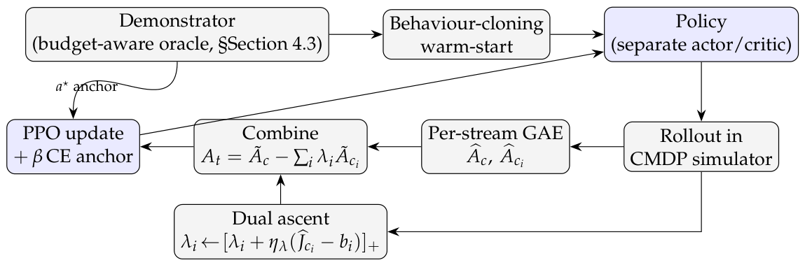
Our goal is a dispatcher that meets each day’s incoming demand at low operating cost while keeping the day’s carbon emissions and service shortfalls within the limits the operator commits to. We obtain such a dispatcher in three steps, which this section develops in turn. We first turn the firm carbon and service limits into prices that the policy responds to so that the operator never has to hand-pick penalty weights and the carbon cap acts as an active constraint on the expected budget rather than a soft penalty; the price on carbon emerges from the optimization and reflects how scarce the budget is on a given day. We then make the price signal usable by a learning agent so that the pursuit of low carbon does not silently erase the incentive to keep cost down. Finally, we equip the training procedure to discover that serving a heterogeneous city well requires the routing of different orders through different channels, a pattern the basic procedure does not find on its own. Throughout, the underlying policy optimizer is proximal policy optimization (PPO), chosen for its stability on the long, stochastic delivery episodes we consider, but the contributions are not specific to it. Figure 2 summarizes the resulting training pipeline.

4.1. Constrained Policy Optimization

Attach to each operating limit a price (${\lambda }_i\ge 0$), and form the Lagrangian as

$$\mathcal{L}(\pi ,\mathbf{\lambda })=J_c\left(\pi \right)+{\displaystyle \sum _{i=1}^{N_c}}{\lambda }_i\left(J_{c_i}\left(\pi \right)-b_i\right),{\lambda }_i\ge 0;$$

the saddle point (${min}_{\pi }{max}_{\lambda \ge 0}\mathcal{L}$) is solved by an alternating primal–dual update. The policy step is a PPO-clip update on the per-stream-standardized advantage:

$${\tilde{A}}_{c,t}=\frac{{\widehat{A}}_{c,t}-{\mu }_c}{{\sigma }_c},{\tilde{A}}_{c_i,t}=\frac{{\widehat{A}}_{c_i,t}-{\mu }_{c_i}}{{\sigma }_{c_i}},A_t={\tilde{A}}_{c,t}-\sum _i{\lambda }_i{\tilde{A}}_{c_i,t},$$

where ${\widehat{A}}_{c,t}$ and ${\widehat{A}}_{c_i,t}$ are GAE estimates on the cost and constraint-cost streams and $(\mu ,\sigma )$ are batch statistics; standardizing each stream before combination keeps the cost gradient from being suppressed when $\lambda$ grows. The dual step is projected gradient ascent, i.e.,

$${\lambda }_i^{(k+1)}={\left[{\lambda }_i^{\left(k\right)}+{\eta }_{\lambda }\left({\widehat{J}}_{c_i}\left({\pi }_{\theta }\right)-b_i\right)\right]}_{+}\wedge {\lambda }_{max},$$

with ${\widehat{J}}_{c_i}$ representing a Monte-Carlo estimate from completed rollout episodes and ${\lambda }_{max}=50$. The dominant multiplier (${\lambda }_C$) is warm-started at a small positive value (

Table 1. Hyperparameters We have revised the section citation format and removed the links. of the policy and dual updates.

Group	Setting
Policy network (base)	17 → 128(tanh) → 128(tanh) → {policy logits, $V_c$, $V_{c_1:c_4}$}; shared backbone for the base Lag-PPO and PPO runs
PPO	$\gamma =0.99$, GAE $\lambda =0.95$, clip $ϵ=0.2$, batch 4096, minibatch 256, $E=10$ epochs
Optimizer	Adam, ${\eta }_{\theta }=3\times {10}^{-4}$, gradient clip $0.5$
Lagrangian	${\eta }_{\lambda }=5\times {10}^{-3}$, ${\lambda }_{max}=50$, ${\lambda }^{\left(0\right)}=[0.5,0.1,5.0,5.0]$ (carbon, TW, drone, metro); per-order runs use $[0.5,0.1,0,0]$
Demonstration-regularized (Section 4.3)	separate actor/critic trunks (each $17\to 128\to 128$); BC warm-start 40 epochs; critic warm-up $W=10$ updates; demo weight $\beta =2.0$; entropy bonus off; fine-tune ${\eta }_{\theta }={10}^{-4}$
Hardware	Single NVIDIA RTX 4090, ∼15 min per 300k-step run

); the safety multipliers take a fixed default, set to zero in the per-order experiments of Section 5.3, where those constraints are non-binding.

4.2. Algorithm Pseudocode

Algorithm 1 adopts a Lagrangian PPO framework with a spatiotemporal carbon-factor model and per-stream normalization. In each iteration, it samples a trajectory, computes GAE advantages for each cost stream, and standardizes them per stream. The carbon advantage and safety advantages are then combined via multipliers ${\lambda }_i$, re-standardized, and used for PPO policy and value updates. Finally, multipliers are updated based on the average safety cost to approach budgets $b_i$ with a hard cap. The process iterates until convergence, returning the final policy and multipliers.

Algorithm 1 Lagrangian-PPO  [30] with the spatiotemporal carbon-factor model and per-stream normalization

Require:  CMDP ${\mathcal{M}}_C$, initial policy $\theta$, value heads ${\varphi }_c,{\varphi }_{c_i}$, multipliers ${\mathbf{\lambda }}^{\left(0\right)}$, budgets $\left\{b_i\right\}$, rates ${\eta }_{\theta },{\eta }_{\lambda }$, clip ${\lambda }_{max}$    1: Initialize ${\lambda }_C^{\left(0\right)}\leftarrow$ small positive warm-start; ${\lambda }_j^{\left(0\right)}\leftarrow$ fixed default for safety constraints (Table 1)    2: for  $k=1,2,\dots$ do    3:     Sample rollout ${\tau }_k$ of length T from ${\pi }_{\theta }$    4:     Compute per-step $c_t,\left\{c_{i,t}\right\}$ from the simulator    5:     Compute ${\widehat{A}}_{c,t},\left\{{\widehat{A}}_{c_i,t}\right\}$ via GAE on each stream independently    6:     Standardize each stream: ${\tilde{A}}_{c,t}\leftarrow ({\widehat{A}}_{c,t}-{\mu }_c)/{\sigma }_c$, similarly for each i    7:     Combine: $A_t\leftarrow {\tilde{A}}_{c,t}-{\sum }_i{\lambda }_i^{\left(k\right)}{\tilde{A}}_{c_i,t}$    8:     Re-standardize $A_t$ across the batch for stable PPO updates    9:     for epoch = 1, …, E do  10:         Update $\theta$ by PPO-clip with advantage $A_t$  11:         Update value heads ${\varphi }_c$, $\left\{{\varphi }_{c_i}\right\}$ by MSE regression  12:     end for  13:     Estimate ${\widehat{J}}_{c_i}\leftarrow$ episode mean of ${\sum }_t{c}_{i,t}$ over rollout  14:     Update each multiplier: ${\lambda }_i^{(k+1)}\leftarrow min({\lambda }_{max},{[{\lambda }_i^{\left(k\right)}+{\eta }_{\lambda }({\widehat{J}}_{c_i}-b_i)]}_{+})$  15: end for  16: return  ${\theta }^{*},{\lambda }^{*}$

4.3. Demonstration-Regularized Fine-Tuning

The fine-tuning step uses a non-learning demonstrator (${\pi }^{★}$) with access to the per-order emission model. For order $o_t$, with a remaining per-order allowance of ${\widehat{b}}_t=(B_C-{\widehat{C}}_{\le t})/N_{\mathrm{remaining}}$ and affordable channels expressed as $\mathcal{F}\left(o_t\right)=\{m:g(o_t,m,t)\le {\widehat{b}}_t\}$,

$$a^{★}\left(o_t\right)=\left\{\begin{array}{cc}arg\underset{m\in \mathcal{F}\left(o_t\right)}{min}c(o_t,m),\hfill & \mathcal{F}\left(o_t\right)\ne \varnothing \hfill \\ arg\underset{m\in \{0,1,2\}}{min}g(o_t,m,t),\hfill & \mathrm{otherwise}.\hfill \end{array}\right.$$

Training proceeds in four steps:

(1)

Roll out ${\pi }^{★}$ on training episodes and collect demonstrations (${\mathcal{D}}_{★}=\left\{(s,a^{★})\right\}$).

(2)

Pre-train ${\pi }_{\theta }$ by behaviour cloning: minimize ${\mathbb{E}}_{(s,a^{★})\sim {\mathcal{D}}_{★}}[-log{\pi }_{\theta }(a^{★}\mid s)]$.

(3)

Use separate trunks for actor and critic models; for the first W updates, train only the value heads, holding the cloned policy fixed.

(4)

Fine-tune with the constrained update of Section 4.1 under the augmented objective, i.e.,

$${\mathcal{L}}_{\pi }\left(\theta \right)={\mathcal{L}}_{\mathrm{PPO}}\left(\theta \right)+\beta {\mathbb{E}}_{(s,a^{★})\sim {\mathcal{D}}_{★}}\left[-log{\pi }_{\theta }(a^{★}\mid s)\right],$$

with the entropy bonus set to zero.

At deployment, ${\pi }_{\theta }$ acts based on its own observations; ${\pi }^{★}$ is not invoked.

5. Numerical Experiments

5.1. Experimental Setup

The simulator is a custom Gymnasium environment. It uses a 30 × 30 grid city with one depot at $(15,15)$, six metro stations along a vertical trunk line, and 16 drone landing pads on a 4 × 4 sub-grid. Order arrival is Poisson with a rate of $0.4$/min, yielding ∼192 orders per 480 min (8 h) episode. The carbon budget is $B_C=750$ unless stated otherwise, the time-window budget is $B_{TW}=50$, and drone-energy and metro-capacity budgets are zero (strict). Speeds are 0.5/1.5/3.0 grid cells per minute for truck/drone/metro respectively, and the drone range is 12 grid cells. Hyperparameters of all algorithms are summarized in Table 1. Unless noted otherwise, every reported policy is evaluated by deterministic action selection (argmax) over the same 50 held-out stochastic days (seed 1234), and the per-channel reference rows in each table are the corresponding deterministic single-channel policies under the identical evaluation set. Channel-use percentages are integer-rounded; small (≤1%) inter-table differences for the same policy arise from rounding and depending on whether the percentages are computed per seed, then averaged or pooled across seeds, not from different evaluation runs.

How the carbon budget is set in each experiment. In every experiment except that described in Section 5.4 (which sweeps the cap), we set $B_C$ so that the budget-aware reference oracle runs within about $5\%$ of the cap. This makes the constraint active rather than nominal, and it is the operational regime in which a constrained learner is worth evaluating: with a slack cap, cost-only PPO would already be feasible; with a punishingly tight cap, no policy can serve demand. Concretely, $B_C=720$ on the 30 × 30 design instance, $B_C=450$ on the small 22 × 22 city, $B_C=1300$ on the large 40 × 40 city, $B_C=700$ on the Nanjing-inspired instance, and $B_C\in \{600,720,840\}$ in the cap-slider study.

5.2. Compared Algorithms

We compare the following. B0 Single-channel (deterministic): always uses mode $k\in \{0,1,2\}$, giving the three single-channel reference operations; B1 PPO (penalty-free) [33]: standard PPO that minimizes only $-c$, with the carbon and service limits absent from the objective; B2 Lag-PPO + demonstration-regularized fine-tuning (proposed). For each instance, we additionally compute an offline clairvoyant optimum with the method proposed by Gurobi [34], which assigns every order to a channel by exactly solving the day’s multiple-choice knapsack with full knowledge of demand and per-order emissions; it is an upper bound on achievable performance rather than a deployable online policy. All learned methods are trained with $n=3$ random seeds and evaluated under the common protocol (argmax, 50 days, seed 1234); across-seed variance is small throughout.

5.3. Serving Heterogeneous Demand

A real city’s delivery needs vary order by order: distance to the depot, proximity to a metro line, and local congestion all differ across neighbourhoods, and so does the cheapest channel that respects the carbon cap. We instantiate this with a two-line metro network with a cross-line transhipment surcharge, two clustered landing-pad groups, and carbon hotspots amplifying both road and drone legs. A per-order diagnostic for this instance shows that each of the three channels is the carbon-minimizing choice for a sizeable, non-trivial subset of orders and that a budget-aware reference operation built on this fact meets the day’s demand within the carbon cap. Committing, instead, to any single channel either over-emits (the cheap road-only operation breaches the cap by 231 units) or over-spends (the lowest-carbon single channel costs 3885, which is more than $30\%$ above the per-order assignment); the demand cannot be served well by a single channel (

Table 2. Per-order channel assignment and design demand (∼193 orders/day, $B_C=720$). The three single-channel reference operations cannot serve the day’s demand within the cap: road-only is the cheapest but breaches the cap by 231 units, while the lowest-carbon single channel costs over $30\%$ more than the budget-aware reference. Both the reference and our learned policy serve demand within the cap by selecting a different channel for each order, conditioned on its destination, deadline, and remaining-budget state; our policy improves on its behaviour-cloned start (cost $2988\to 2966$ at the same carbon level), which shows that the fine-tuning genuinely solves the constrained problem rather than imitating the successful policy.

Operation	Cost	Carbon	Carbon Viol.
Road only	2879	951	231
Road+drone only	3427	816	98
Metro+road+drone only	3885	982	262
Budget-aware reference (oracle)	2928	720	21
Behaviour-cloned start	2988	727	28
Ours ($\mathit{n}=\mathbf{3}$)	$\mathbf{2966}\pm \mathbf{3}$	$\mathbf{727}\pm \mathbf{0}.\mathbf{5}$	$\mathbf{28}\pm \mathbf{0}.\mathbf{3}$

).

Our method serves this demand within the cap by deciding the channel for each order based on its state. Across $n=3$ seeds, the trained policy attains a cost of $2966\pm 3$ at emissions of $727\pm 0.5$ against the budget of 720, with a small day-to-day overshoot ($28\pm 0.3$) driven by demand variance rather than by overuse of any high-carbon channel; the carbon price settles at ${\lambda }_C\approx 5$, consistent with an interior (constraint-active) solution. The policy improves on its behaviour-cloned start (cost of $2988\to 2966$ at the same emissions), so fine-tuning solves the constrained problem by observation rather than by imitating the reference operation. The deployed policy maps state directly to channel and never queries the emissions model at decision time.

To make the distinction between average and per-day compliance explicit,

Table 3. Daily-emissions distribution for the design instance ($B_C=720$), aggregated over 3 seeds × 50 evaluation days = 150 realisations.

Statistic	Value
Mean daily emissions	$726.6$
95% CI on mean	$[717.2,736.0]$
Std across days	$58.7$
Median daily emissions	$721.0$
90th/95th/99th percentile	$801.9/826.3/848.5$
Days within cap (feasibility rate)	$48\%$
Days exceeding $1.05B_C/1.10B_C$	$34.7\%/12.0\%$
Mean overshoot on infeasible days	$53.2$
Max overshoot on infeasible days	$132.7$

summarises the full daily-emissions distribution over 150 realisations (3 seeds $\times 50$ days) of the design instance. The mean daily emissions are $726.6$, with a $95\%$ CI of $[717.2,736.0]$ that brackets the cap of 720, and the median day sits essentially at the cap: the constraint is honoured in expectation. However, only $48\%$ of individual days stay at or below the cap. Therefore, the method should be interpreted as controlling the expected or average carbon budget, not as guaranteeing per-day compliance; a risk-sensitive extension (e.g., CVaR or chance constraint) would be needed to upgrade this to a per-day guarantee, which we leave to future work.

Robustness to demand-scale variation. A real operator’s daily order volume is not fixed. To see whether the same policy continues to serve demand well as the day’s volume changes, we keep the trained policy and carbon budget unchanged and conduct a zero-shot evaluation at five Poisson arrival rates ranging from $0.2$ to $0.6$ per minute, corresponding to roughly 100 to 290 orders per day (

Table 4. Demand-scale robustness ($n=3$ seeds, 50 days per rate under the common protocol, and $B_C=720$ (unchanged)). The policy is trained at a rate of $0.4$/min and subject to zero-shot zero-shot evaluation at the other rates; the row at $0.4$ reproduces the design-rate result of Table 2. Across a $3\times$ range of daily volume, the policy keeps emissions as close to the cap as the channels physically allow; feasibility holds at the design rate and lighter, and the policy degrades gracefully beyond it.

Arrival Rate (/min)	Orders/day	Cost	Carbon	Carbon Viol.
$0.2$	98	1466	418	$0.0$
$0.3$	146	2201	585	$0.0$
$0.4$ (training)	193	$2966\pm 3$	727	$27.7$
$0.5$	241	3851	896	176
$0.6$	289	4721	1073	353

). The policy adapts to demand without being retrained. On lighter days, the per-order share of the carbon budget is generous, the cheap road channel can be used freely, and emissions stay well under the cap. As daily demand grows, the per-order budget tightens, and the policy reallocates toward the lower-carbon channels to push the day’s emissions as low as the available channels allow. Feasibility is maintained up to the design rate and degrades gracefully beyond it: under very heavy demand, even the cleanest reachable assignment exceeds the budget, and the carbon cap can no longer be met. Thus, the same scheduler covers a $3\times$ range of daily volumes; the operator’s choice is whether to absorb the resulting cost increase or scale up the carbon budget when demand surges.

5.4. Operator’s Carbon-Cap Slider

A sustainability operator’s principal lever is the carbon cap itself: How strict can the cap be made before the cost becomes uncomfortable, and how does the scheduler respond? We test this by retraining our method at two additional cap levels around the design value, i.e., $B_C\in \{600,720,840\}$ (a ± 17% band), keeping everything else unchanged (

Table 5. Operator’s carbon-cap slider for the per-order-heterogeneous instance. Each row is a separately trained policy at the listed cap; all other settings are unchanged (50 days, seed 1234, and n seeds, as listed). Cost moves smoothly as the cap moves; the policy reallocates toward lower-carbon channels as the cap tightens, until the all-greenest reachable assignment’s emissions floor (around 700) prevents further reduction.

Cap ${\mathit{B}}_{\mathit{C}}$	vs. Design	Cost	Carbon	Carbon Viol.
600 ($n=2$)	$-17\%$	$3015\pm 1$	711	111
720 ($n=3$, design)	0	$2966\pm 3$	727	28
840 ($n=2$)	$+17\%$	$2876\pm 2$	766	$2.4$

). The policy responds in the expected operational direction. Loosening the cap to 840 lets the policy lean on the cheap road channel; cost falls by $3\%$ to 2876, and carbon stays comfortably below the cap, with a small residual overshoot of only $2.4$ units. At the design cap of 720, the policy hugs the cap at a cost of 2966, with carbon at 727. Tightening the cap to 600 pushes the policy toward the lower-carbon channels; cost rises only by $1.7\%$ to 3015, but carbon settles at 711 rather than 600 because the all-greenest reachable assignment for this instance has an emissions floor near 700. The operator’s reading is direct: a ± 17% change in target costs only $\pm 3\%$ in operations within the physically attainable range, but the cap cannot be pushed below the emissions floor without changing the fleet (a deeper metro share, more pads, and electrified road segments). The same algorithm, applied to whatever cap the operator chooses, produces the cap-appropriate operating point.

5.5. Why the Conventional Penalty Approach Is Not Enough

We replace the constrained objective with the fixed-weight penalty reward ($r=-(c+\alpha g)$) and train PPO at $\alpha \in \{1,3,5,10,20\}$ on the per-order instance, with all other settings unchanged (

Table 6. Fixed-weight penalty PPO at five weights for the per-order instance ($B_C=720$). The policy converges to a single channel at every tested weight: road at $\alpha =1$ and road+drone for all $\alpha \ge 3$. No weight setting reaches a per-order assignment; our adaptive constrained learner does so at lower cost than the cheapest near-feasible fixed-$\alpha$ point.

$\mathit{\alpha }$	Cost	Carbon	Carbon Viol.	Comment
1	2879	951	231	road-only (carbon-infeasible)
3	3427	816	98	road+drone collapse
5	3427	816	98	,,
10	3427	816	98	,,
20	3427	816	98	,,
Ours (adaptive, ${\mathbf{\lambda }}_{\mathbf{C}}\approx \mathbf{5}$)	$\mathbf{2966}$	$\mathbf{727}$	$\mathbf{28}$	per-order, near-feasible

). At $\alpha =1$, the converged policy uses road only (cost, 2879; carbon, 951; violation, 231); for $\alpha \ge 3$, it uses road+drone only (cost, 3427; carbon, 816; violation, 98). No tested weight yields a per-order assignment or a point that is both feasible and cheaper than 3427. Our adaptive method (Table 2, ${\lambda }_C\approx 5$) attains a cost of 2966 at a violation value of 28.

5.6. Robustness Across City Scales

A real operator does not work in a single fixed city: small towns and large metropolises have different grid extents, different metro and pad densities, and different daily order volumes. To check that the same method serves demand across this range, we train and evaluate it on three instances spanning a $3\times$ scale band (

Table 7. Robustness to city scale: same method, with three instances spanning a $3\times$ size band (50 days per instance, seed 1234). Each city has its own binding carbon budget. The cap is met within a margin set by day-to-day demand variance at every scale, without any per-city tuning.

Scale	Grid/Metro/Pads	Orders/Day	${\mathit{B}}_{\mathit{C}}$	Cost	Carbon	Carbon Viol.
Small	$22\times 22$/4/8	146	450	1926	454	$+19$
Medium	$30\times 30$/6/16	193	720	$2966\pm 3$	727	$+28$
Large	$40\times 40$/8/24	241	1300	4884	1277	$+22$

). The small city is a $22\times 22$ grid with four metro stations and eight pads carrying ∼146 orders/day; the medium city is the $30\times 30$ default of Section 5.3 (∼193 orders/day); and the large city is a $40\times 40$ grid with eight metro stations and twenty-four pads carrying ∼241 orders/day. Each instance has its own binding carbon budget (set so the budget-aware reference operation runs near the cap). The method finds a near-feasible per-order assignment in all three. At every scale, the policy stays within roughly the same margin of the cap (18–28 units of overshoot, all driven by day-to-day demand variance), and the cost scales with demand as expected. The same training recipe and hyperparameters are used at each scale; no per-city tuning is needed.

Sensitivity to demonstration quality. The demonstration-regularized recipe uses an oracle demonstrator (Section 4.3) at training time. To assess how much the final policy depends on the demonstrator’s quality, we re-trained the method under three degraded demonstrator settings and evaluated with the common protocol (

Table 8. Sensitivity of the demonstration-regularized policy to demonstrator quality (design instance, $B_C=720$, 50 evaluation days, seed 1234). “Clean” is the study baseline of Table 2 aggregated over three seeds; each degraded condition is a single training run started from a corrupted demo file. Noise f replaces a fraction (f) of demo actions with a different uniformly random action; “partial 50%” drops half of the demo trajectories.

Demo Condition	Cost	Carbon (Mean)	Feas. Rate	$\mathbf{\Delta }$Feas. vs. Clean
Clean (paper baseline, $n=3$)	2967	$726.6$	$48\%$	—
Noise 10%	2974	$740.8$	$38\%$	$-10$ pp
Noise 30%	2997	$746.5$	$30\%$	$-18$ pp
Partial (drop 50%)	2985	$734.7$	$44\%$	$-4$ pp

). Small label noise ($10\%$) and the dropping of half the demo trajectories are largely absorbed by the fine-tuning: cost stays within $0.6\%$ of the clean baseline, and the mean daily emissions grow by 8–14 units, with per-day feasibility dropping by only 4–10 percentage points. Heavier $30\%$ label noise degrades feasibility further ($30\%$) while still keeping cost within $1.0\%$. This confirms the design intent of the recipe: behaviour cloning provides an initialization, not a target, and the anchoring weight of $\beta =2.0$ is not large enough to dominate the on-policy PPO gradient. We note that the demonstrator itself is a per-city artefact (it encodes which channel is the carbon-minimising choice for orders in that specific city’s geometry) and should be regenerated when moving to a new city rather than being reused across cities; regenerating it is cheap, since the underlying budget-aware heuristic takes only minutes to run once.

Deployment cost and scalability. The deployed policy is a single small MLP ($38,664$ parameters, obs-dim 17, two $17\to 128\to 128$ trunks, and three heads). One forward-pass on the design instance is 489 $\mathsf{\mu }$s, on average, on a single-thread CPU (p99 $1.68$ ms), 13 $\mathsf{\mu }$s per decision when the same CPU processes a batch of 64 (p99 46 $\mathsf{\mu }$s), and $4.2$ $\mathsf{\mu }$s per decision on an RTX 4090 with a batch of 1024 (p99 $8.4$ $\mathsf{\mu }$s). All of these are three to four orders of magnitude below the shortest realistic order inter-arrival time in urban delivery, which sits in the second-to-minute range at any realistic city rate. Since the observation is a fixed 17-dimensional feature vector, regardless of city geometry, the per-decision cost does not grow with the number of metro stations, drone pads, or orders per day; only the nearest-station and nearest-pad lookups grow (naïvely, $O(K_M+K_L)$ per order; trivially indexed to $O(logK)$). Training is a one-time offline cost that scales linearly with the training-step budget. The baseline recipe uses ∼180,000 PPO steps (equivalently, 43 rollout iterations of 4096 steps each) and takes ∼15 min on a single RTX 4090 for the $30\times 30$ instance and ∼20 min for the $40\times 40$ large-city instance. Therefore, practical logistics systems with thousands of orders per day remain well within reach.

Hyperparameter selection. The demonstration-regularized recipe has three settings that materially affect the outcome, and we make the reasoning behind them explicit here rather than treating them as tuned magic numbers. The remaining PPO settings are the standard values reported in the original PPO paper [33] and were not modified. Demonstration weight $\beta$: The anchoring term must be strong enough to prevent the fine-tuning from immediately abandoning the demo prior (which happens without anchoring; see the noise variants in Table 8 for the effect of a partially corrupted prior) but small enough that on-policy PPO can still correct the demo where it is imperfect; the value of $\beta =2.0$ was chosen so that the anchoring loss and the PPO surrogate loss are of comparable magnitude at initialization. Behaviour-cloning warm-start epochs: We use forty epochs, chosen so that the BC cross-entropy loss visibly plateaus before hand-off to the constrained PPO loop; the demo dataset has $38,684$ state–action pairs, and forty full passes provide a comfortable margin above the point where the BC loss saturates. Lagrangian learning rate (${\eta }_{\lambda }=5\times {10}^{-3}$): The Lagrangian learning rate is chosen so the dual update completes within the first quarter of training but does not oscillate against the primal update. Direct benchmarking against alternative values in a full sweep is left to future work, but the demo-quality ablation in Table 8 indirectly shows the recipe is not brittle: substantial perturbations to the demonstrations (which effectively change how strongly $\beta$ has to work) still yield well-behaved training.

5.7. Semi-Real Case Study: A Nanjing-Inspired Instance

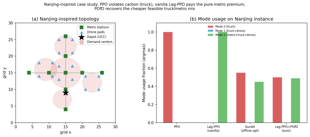
The settings above are synthetic. To test whether the same behaviour appears on a realistic city geometry, we built a Nanjing-inspired instance (Figure 3a): the metro network follows Nanjing’s core cross topology (Line 1 (north–south) × Line 2 (east–west), interchanging at the Xinjiekou CBD); demand is population-weighted over the CBD and four sub-centres (Hexi, Jiangning, Xianlin, and Chengnan) rather than uniform; and the depot is a semi-central urban consolidation centre south of the core. This geometry creates a genuine cost–carbon tension: truck-direct delivery is cheapest (cost of 2156, and carbon emissions of 1025) but carbon-heavy, whereas the metro chain halves carbon (505) at a 13% cost premium (2435). The carbon budget $B_C=700$ excludes the truck-only corner (

Table 9. Nanjing-inspired instance ($B_C=700$). All rows are evaluated on the same 50 stochastic days (seed 1234); learned policies act greedily (argmax). The first block lists reference points: the two single-channel policies and the offline clairvoyant optimum from a Gurobi mixed-integer program with full knowledge of the day’s orders and per-order emissions. The second block lists learned online policies; cost-only PPO and the plain constrained policy converge exactly to the road-only and metro-chain references respectively, so those rows coincide. Our method learns a feasible per-order assignment within $1.3\%$ of the offline optimum cost while being online and model-free.

	Method	Cost	Carbon	Carbon Viol.
Ref.	Road-only	2110	1008	308
	Metro-chain	2359	491	0
	Gurobi offline optimum	1791	596	0
Learned	PPO (cost-only)	2110	1008	308
	Lagrangian-PPO (plain)	2359	491	0
	Ours ($\mathit{n}=\mathbf{3}$)	$\mathbf{1815}\pm \mathbf{1}$	$\mathbf{569}\pm \mathbf{4}$	$\mathbf{0}.\mathbf{0}$

).

The result mirrors the synthetic findings on a realistic geometry, and the additional reference points sharpen the picture. Cost-only PPO commits to road delivery and breaches the carbon cap by 308 units; a plain constrained policy is feasible but commits to all-metro, paying the pure-metro premium (cost of 2359). To bound how well any policy could do, we solve the day’s assignment exactly with Gurobi [34], given full knowledge of every order and its per-channel cost and emissions; this offline, clairvoyant optimum attains a cost of 1791 within the carbon budget, which is the best cost any feasible assignment can reach. We note that it is exact for the stylized per-order channel-assignment model used throughout, not for the full operational dispatch problem with routing and timing. It is, in any case, not a policy an operator can run: it requires the whole day’s demand and an exact emissions model in advance and re-solves a mixed-integer program for each instance. Our method, deciding each order online and without any analytical emissions model, learns a per-order assignment at a cost of $1815\pm 1$ (carbon of $569\pm 4$, feasible, and $n=3$ seeds), which is within $1.3\%$ of this offline optimum. Thus, it serves demand $23\%$ more cheaply than the plain constrained policy at comparable feasibility while needing none of the demand foresight or the emission model the offline optimum requires. In a realistic city where the cheapest and most carbon-feasible operations differ and where serving demand well calls for a per-order channel assignment rather than a single channel, the online model-free policy does what neither a single-channel rule nor an offline solver can deliver to an operator. In this instance, the realized assignment is effectively two-channel (road and metro): because the drone range is generous and pads are well placed, the road-plus-drone channel is rarely the cheapest carbon-feasible option for any order, so the policy concentrates on the road/metro trade-off; the full three-channel per-order assignment is exercised in the synthetic study of Section 5.3.

6. Discussion

The experiments draw a clear operational lesson about when per-order channel assignment matters. In a uniform city or in one whose carbon hotspots do not change which channel is cheapest for an order, committing to the lowest-carbon channel for everything is a sound policy, and our method settles there. But real cities are not uniform: proximity to a metro line, to the depot, and to congested districts varies sharply from one neighbourhood to the next, so the channel that serves an order at the lowest cost under the carbon budget differs from order to order. In such a city, the operation that best meets demand is a per-order assignment, and what a learning scheduler offers is that it can discover and apply such an assignment from experience, without the operator hand-specifying which neighbourhoods should use which channel. The contribution of the demonstration-regularized scheme is to make a constrained learner actually reach this operation, which it does not do when left to explore on its own. The operator-facing tests of Section 5.3, Section 5.4, Section 5.5 and Section 5.6 sharpen the same point along three deployment axes: the same trained scheduler tracks a $\pm 17\%$ change in the carbon target, a $3\times$ change in daily order volume, and a $3\times$ change in city scale without per-instance tuning, whereas the conventional fixed-weight penalty PPO of Section 5.5 collapses to a single channel at every tested weight and never finds the per-order assignment at all.

A natural question for a practitioner is when to prefer a learned scheduler over a simple rule that assigns each order to a channel via a hand-built formula. Such a rule is attractive when the carbon and cost of every channel can be computed in advance and the operating environment is stable, and in that case, it is hard to beat. However, its assumptions are exactly what fail in practice: real grid-carbon intensity, metro timetables, and traffic shift depending on the weather, the hour, and the season and are rarely available as a clean formula. The learned scheduler needs no such formula and adapts to conditions it observes as the day unfolds; it also extends without redesign if the operator later wants to decide on routes, timing, or transfer points jointly rather than only the channel.

Transferability to other cities. The CMDP formulation, the Lagrangian-PPO training loop, and the observation-space design are city-agnostic: they contain no reference to any specific city’s geometry and require no changes to move to a new city. However, four instance-level components must be re-instantiated per city: (i) the metro topology (station coordinates and inter-station connectivity), (ii) the location of the depot or urban consolidation centre, (iii) the demand distribution used at training time (either a uniform prior over the grid or, when available, a population-weighted mixture), and (iv) any city-specific carbon-intensity map (the hotspots and cleanspots that induce spatial heterogeneity in $\beta \left(r\right)$). In the accompanying code repository, we provide a template that reduces this re-instantiation to filling in four data structures in the environment class; the Nanjing-inspired instance in Section 5.7 was built this way in fewer than 100 lines of Python3.14. The city-scale robustness study in Section 5.6 demonstrates that the same training recipe and hyperparameters transfer across a $3\times$ scale band without per-city tuning, which is indirect evidence of transferability, but does not replace external validation on a second real city.

Deployment considerations. Four practical points arise when moving from a stylized environment to real operations. Data acquisition: At decision time, the policy observes only state features already routinely available in a fleet-management system (order destination, remaining budget, current time, nearest metro station and pad); no additional live feed is required. Integration with the metro operator: Our current formulation treats the per-hour metro capacity as a static budget; production use would replace this with a real-time capacity feed from the metro authority. Operational drone restrictions: Our environment enforces range but neither no-fly airspace nor weather-based groundings. Adding a no-fly mask and a drone-availability flag to the state is straightforward and does not change the algorithm. Unexpected disruptions: Because the policy is state-dependent, it already responds to disruptions that appear in state (an exceeded subway hour bucket triggers a reallocation away from metro); disruptions that are not in state, such as a fleet-wide drone grounding, would require an availability flag added to the observation. The broader institutional context is also relevant. Real-time AI-driven multimodal logistics depend on smart-city infrastructure, data-sharing between the operator and the metro authority, and the regulatory framework governing drone airspace and freight-metro co-use [35]; these are pre-requisites for deployment that our algorithmic contribution does not, by itself, resolve.

Assumptions and limitations. We consolidate the study’s limitations here. (1) Order arrivals are Poisson; real order streams exhibit weekly and hourly seasonality and correlated bursts that our model does not capture. Consumer demand for last-mile delivery is also shaped by the broader digital marketplace and by the volatility of consumer attention [36], which enters the scheduler only through the parametric arrival process. (2) Destinations are drawn from parametric distributions (uniform or Nanjing five-centre mixture) rather than from operational records. (3) Transfer-station and pad selection uses a nearest-neighbour heuristic; joint routing, timing, and transfer-point optimization is left to future work. (4) All four operational constraints are represented, but in the instance parameters reported in Section 5.1, only the carbon and time-window constraints are tightly binding; drone range and metro-station capacity are slack. Constructing instances in which they bind is a direct next step. (5) The environment is simulated: there is no live road-network router, no metro timetable, no live grid-carbon feed, no airspace constraints, and no weather-driven disruptions. (6) The learned per-order policy leaves a residual carbon overshoot driven by day-to-day demand variance; here, the expected-value carbon constraint targets the mean at the cap and tolerates this variance, so a risk-sensitive constraint that bounds the upper tail of emissions (for example, a CVaR or chance constraint) is the appropriate tool, and it becomes especially important when emissions are non-stationary across days. We leave this risk-sensitive extension to future work. The present results validate the approach on carbon and service; they do not constitute a finished operational tool.

7. Conclusions

This study addressed how a city logistics operator can meet daily delivery demand at low cost while holding emissions and service shortfalls within firm limits, using a fleet that combines road vehicles with metro freight and last-mile drones. We framed the operator’s real-time channel-selection decision as a constrained Markov decision process in which the carbon cap and service requirements are explicit expected-value constraints on the daily budget rather than tunable penalty terms and solved it with a Lagrangian deep reinforcement-learning method that prices those constraints automatically rather than asking the operator to tune penalty weights. On synthetic city instances, the method reduced carbon-budget and time-window violations by roughly two orders of magnitude relative to a penalty-free scheduler with a modest increase in operating cost, leaving only a small residual overshoot driven by day-to-day demand variance rather than by any systematic breach.

The study’s main operational finding is that, in a city whose delivery economics vary across neighbourhoods, no single channel serves demand best. When the cost and carbon of each channel differ across the map, the policy that best meets demand within the carbon budget routes different orders through different channels, and a plain constrained learner does not discover this on its own. Our demonstration-regularized training scheme lets it do so, producing a per-order assignment that serves demand more cheaply than committing to any one channel while holding emissions close to the cap. A case study built from Nanjing’s metro topology and population-weighted demand confirmed the same behaviour on a realistic city geometry, where the learned road-and-metro per-order assignment served demand markedly more cheaply than any single-channel policy at comparable feasibility and within $1.3\%$ of an offline clairvoyant optimum while needing no demand foresight or emission model. Operator-facing tests further showed the same scheduler responds smoothly to a $\pm 17\%$ change in the carbon cap, a $3\times$ change in daily order volume, and a $3\times$ change in city scale, while a hand-tuned fixed-weight penalty PPO collapses to a single channel at every tested weight. Extending the study to a full road network with live metro timetables and to operational demand records and bringing the remaining operating limits into play are the natural next steps toward a deployable tool. External validation on operational data and integration with a live routing engine remain the pre-requisites for deployment.

References

1. Yang, S.; Zhang, W.; Wu, S.; Hu, X. Carbon emissions from express logistics: Estimation and spatial analysis using origin-destination transportation flows. Transp. Policy 2025, 171, 970–985. [Google Scholar] [CrossRef]
2. Gong, Q.; Guo, G. Decoupling relationship between logistics growth and carbon emissions and driving factors in Chongqing: A novel decomposition framework. J. Environ. Manag. 2024, 370, 122931. [Google Scholar] [CrossRef]
3. Hu, W.; Dong, J.; Hwang, B.G.; Ren, R.; Chen, Z. Network planning of urban underground logistics system with hub-and-spoke layout: Two phase cluster-based approach. Eng. Constr. Archit. Manag. 2020, 27, 2079–2105. [Google Scholar] [CrossRef]
4. Brown, J.R.; Bushuev, M.A. Last mile delivery with drones: A carbon emissions comparison. Int. J. Sustain. Transp. 2024, 18, 791–802. [Google Scholar] [CrossRef]
5. Fu, Z.; Yue, J.; Yan, Y. Optimized design of multi-level low-carbon logistics distribution scheme based on two stages. Arch. Transp. 2024, 69, 145–165. [Google Scholar]
6. Guo, J.; Zhao, Q.; Xi, M. Sustainable urban logistics distribution network planning with carbon tax. Sustainability 2022, 14, 13184. [Google Scholar] [CrossRef]
7. Yang, X.; Jiang, H. Research on urban cold chain logistics path optimization considering multi-center and time-varying road networks. IEEE Access 2024, 12, 71331–71348. [Google Scholar]
8. Peng, Y.; Ren, Z.; Yu, D.Z.; Zhang, Y. Transportation and carbon emissions costs minimization for time-dependent vehicle routing problem with drones. Comput. Oper. Res. 2025, 176, 106963. [Google Scholar] [CrossRef]
9. Liu, H.; Zhang, J.; Zhou, Z.; Dai, Y.; Qin, L. A deep reinforcement learning-based algorithm for multi-objective agricultural site selection and logistics optimization problem. Appl. Sci. 2024, 14, 8479. [Google Scholar] [CrossRef]
10. Altman, E. Constrained Markov Decision Processes; Chapman and Hall/CRC: Boca Raton, FL, USA, 1999. [Google Scholar]
11. Peng, Y.; Zhang, Y.; Yu, D.Z.; Luo, Y. Multiobjective route optimization for multimodal cold chain networks considering carbon emissions and food waste. Mathematics 2024, 12, 3559. [Google Scholar] [CrossRef]
12. Chen, W.; Zhang, D.; van Woensel, T.; Xu, G.; Guo, J. Green vehicle routing using mixed fleets for cold chain distribution. Expert Syst. Appl. 2023, 233, 120979. [Google Scholar] [CrossRef]
13. Chen, J.; Liao, W.; Yu, C. Route optimization for cold chain logistics of front warehouses based on traffic congestion and carbon emission. Comput. Ind. Eng. 2021, 161, 107663. [Google Scholar] [CrossRef]
14. Guo, X.; Zhang, W.; Liu, B. Low-carbon routing for cold-chain logistics considering the time-dependent effects of traffic congestion. Transp. Res. Part D Transp. Environ. 2022, 113, 103502. [Google Scholar] [CrossRef]
15. Delle Donne, D.; Alfandari, L.; Archetti, C.; Ljubić, I. Freight-on-Transit for urban last-mile deliveries: A strategic planning approach. Transp. Res. Part B Methodol. 2023, 169, 53–81. [Google Scholar] [CrossRef]
16. Hong, I.; Kuby, M.; Murray, A.T. A range-restricted recharging station coverage model for drone delivery service planning. Transp. Res. Part C Emerg. Technol. 2018, 90, 198–212. [Google Scholar] [CrossRef]
17. Chauhan, D.; Unnikrishnan, A.; Figliozzi, M. Maximum coverage capacitated facility location problem with range constrained drones. Transp. Res. Part C Emerg. Technol. 2019, 99, 1–18. [Google Scholar] [CrossRef]
18. Dell’Amico, M.; Montemanni, R.; Novellani, S. Algorithms based on branch and bound for the flying sidekick traveling salesman problem. Omega 2021, 104, 102493. [Google Scholar] [CrossRef]
19. Perboli, G.; Brotcorne, L.; Bruni, M.E.; Rosano, M. A new model for last-mile delivery and satellite depots management: The impact of the on-demand economy. Transp. Res. Part E Logist. Transp. Rev. 2021, 145, 102184. [Google Scholar] [CrossRef]
20. Schiffer, M.; Walther, G. The electric location routing problem with time windows and partial recharging. Eur. J. Oper. Res. 2018, 260, 995–1013. [Google Scholar] [CrossRef]
21. Bello, I.; Pham, H.; Le, Q.V.; Norouzi, M.; Bengio, S. Neural combinatorial optimization with reinforcement learning. arXiv 2016, arXiv:1611.09940. [Google Scholar]
22. Kool, W.; van Hoof, H.; Welling, M. Attention, learn to solve routing problems! In Proceedings of the International Conference on Learning Representations (ICLR), New Orleans, LA, USA, 6–9 May 2019. [Google Scholar]
23. Nazari, M.; Oroojlooy, A.; Snyder, L.V.; Takáč, M. Reinforcement learning for solving the vehicle routing problem. In Proceedings of the Advances in Neural Information Processing Systems (NeurIPS), Montreal, QC, Canada, 3–8 December 2018. [Google Scholar]
24. Zhang, H.; Wang, Y.; Jiang, M.; Huang, Z.; Pang, K.W.; Liu, Z. Optimizing land-air collaborative operations with environmental considerations. Transp. Res. Part E Logist. Transp. Rev. 2025, 202, 104301. [Google Scholar] [CrossRef]
25. Bayliss, C.; Bektaş, T.; Tjon-Soei-Len, V.; Rohner, R. Designing a multi-modal and variable-echelon delivery system for last-mile logistics. Eur. J. Oper. Res. 2023, 307, 645–662. [Google Scholar] [CrossRef]
26. Cho, Y.H.; Baek, D.; Chen, Y.; Jung, M.J.; Vinco, S.; Macii, E.; Poncino, M. Multi-criteria coordinated electric vehicle-drone hybrid delivery service planning. IEEE Trans. Veh. Technol. 2022, 72, 5892–5905. [Google Scholar]
27. Achiam, J.; Held, D.; Tamar, A.; Abbeel, P. Constrained policy optimization. In Proceedings of the International Conference on Machine Learning (ICML), Sydney, Australia, 6–11 August 2017; pp. 22–31. [Google Scholar]
28. Tessler, C.; Mankowitz, D.J.; Mannor, S. Reward constrained policy optimization. arXiv 2018, arXiv:1805.11074. [Google Scholar]
29. Liu, Y.; Ding, J.; Liu, X. IPO: Interior-point policy optimization under constraints. In Proceedings of the AAAI Conference on Artificial Intelligence, New York, NY, USA, 12 February 2020; Volume 34, pp. 4940–4947. [Google Scholar]
30. Stooke, A.; Achiam, J.; Abbeel, P. Responsive safety in reinforcement learning by PID Lagrangian methods. In Proceedings of the International Conference on Machine Learning (ICML), Virtual, 13–18 July 2020; pp. 9133–9143. [Google Scholar]
31. Jiang, J.; Sheng, D. Multi-period regional low-carbon logistics network planning with uncertain demand. Energy 2025, 331, 137068. [Google Scholar] [CrossRef]
32. Lin, H.J.; Chen, P.C.; Lin, H.P.; Hsieh, I.Y.L. Quantifying carbon emissions in cold chain transport: A real-world data-driven approach. Transp. Res. Part D. Transp. Environ. 2025, 142, 104679. [Google Scholar] [CrossRef]
33. Schulman, J.; Wolski, F.; Dhariwal, P.; Radford, A.; Klimov, O. Proximal policy optimization algorithms. arXiv 2017, arXiv:1707.06347. [Google Scholar]
34. Gurobi Optimization; LLC. Gurobi Optimizer Reference Manual. 2024. Available online: https://www.gurobi.com (accessed on 15 October 2025).
35. Peráček, T.; Kaššaj, M. The Impact of Effective Public Administration and European Digital Connectivity on Building Smart Cities: An Analysis of Legal Frameworks, Policy Initiatives and Transformative Impact in the Emerging Era of Artificial Intelligence. Jurid. Trib. Rev. Comp. Int. Law. 2025, 15, 721–745. [Google Scholar]
36. Ivančík, R.; Nečas, P.; Il’aščíková, L. Attention as a Commodity in the World of Disinformation and Social Media. J. Entrep. Sustain. Issues 2024, 12, 176. [Google Scholar] [CrossRef]
Figure 1. A single order can be served by one of three channels: road-direct (mode 0), a road leg handing off to a drone at a pad (mode 1), or a metro trunk leg followed by a road-and-drone leg (mode 2). Solid lines are road or metro legs, dotted lines are drone flight. The dispatcher picks one channel per order under the carbon budget and service constraints.
Applsci 16 07114 g001
Figure 2. Training pipeline. A budget-aware demonstrator (Section 4.3) warm-starts the policy by behaviour cloning; the policy then alternates rollout, per-stream advantage estimation, λ -weighted combination, and a PPO update with a demonstration-anchoring term, while the dual variables ascend on the measured constraint violations. The demonstrator is used only in training; at deployment, the policy acts based on its own observations.
Applsci 16 07114 g002
Figure 3. Nanjing-inspired case study. (a) Topology: Nanjing’s core metro cross, population-weighted demand centres, drone pads, and a semi-central depot. (b) Mode usage: cost-only PPO uses only trucks (carbon-infeasible); vanilla Lag-PPO collapses to pure metro (feasible but costly); and our demonstration-regularized policy recovers the cheaper feasible truck/metro per-order assignment, recovering the same qualitative truck/metro per-order assignment and approaching the oracle on cost.
Applsci 16 07114 g003