Reduct for Large Datasets: Parallel Multi-Processor Architecture in FPGA

Abstract

This work introduces a parallel architecture that leverages both a Field-Programmable Gate Array (FPGA) and a softcore CPU to accelerate reduct computation for large-scale datasets using rough set theory. The proposed designs were evaluated on two real-world datasets executed directly on the FPGA platform, with dataset sizes ranging from 1000 up to 1,000,000 objects. An equivalent software implementation was used as a reference. Experimental results demonstrate that the hardware-supported reduct generation achieves substantial reductions in computation time compared to the software solution, giving speed-up factors from 5 up to 16 times for the same number of cores both in hardware and software, up to 52 times when comparing hardware four-core approach with single software core solution.

1. Introduction

Major challenge in the development of efficient decision-support systems is the time required to process input data, particularly when dealing with large-scale datasets, commonly referred to as big data. This term encompasses extensive, heterogeneous, and dynamically evolving collections of data whose analysis is computationally demanding yet highly valuable, as it often reveals previously inaccessible patterns or knowledge. A dataset may be regarded as “large” when it exceeds the capabilities of standard analytical tools and widely accessible computational resources [1]. The point at which this occurs depends on the complexity of the algorithms employed and may range from megabytes to terabytes.

Numerous techniques have been proposed to address the computational burden posed by such datasets, with particular emphasis on knowledge discovery and data reduction. Rough set theory represents one such approach, offering a mechanism for reducing the dimensionality of the data by eliminating attributes that do not contribute essential information. Introduced by Z. Pawlak [2], rough set theory extends classical set-theoretic notions to accommodate uncertainty and incompleteness. Two concepts play a pivotal role in this framework: reduct and the core [3]. A reduct is a minimal subset of attributes that preserves the classification capability of the full dataset, while the core consists of attributes that are indispensable and present in every possible reduct. More information about recent research about feature selection and attribute reduction using rough sets approach can be found in [4,5].

Field-Programmable Gate Arrays (FPGAs) provide a reconfigurable hardware platform whose architecture can be adapted to implement custom digital logic, typically using hardware description languages such as VHDL. Their flexibility, together with substantial potential for fine-grained parallelism, makes FPGAs well suited for accelerating rough set computations. As a result, they can serve as high-performance computational units in both embedded and general-purpose systems operating on large datasets.

The primary objective of this study is to develop an FPGA-based architecture for reduct computation, employing specialized processing units capable of executing operations in parallel. Compared with conventional software-based implementations, the proposed solution achieves significantly higher computation speeds, often by several orders of magnitude.

Prior research has predominantly concentrated on software-oriented solutions or algorithms with low computational complexity. For example GPU-, cloud-, and MapReduce-based approaches are practical alternatives to FPGA acceleration for big data processing, primarily due to their flexibility and scalability. GPUs provide high throughput via massive parallelism, making them well-suited for data-intensive workloads, albeit with higher energy consumption and less predictable latency than FPGAs [6]. Cloud platforms enable elastic scaling and easy access to heterogeneous resources without upfront hardware investment [7]. The MapReduce model (e.g., Hadoop, Spark) ensures distributed, fault-tolerant processing, though it may introduce overhead for iterative tasks [8]. Recent research related to this topic is, for instance, [9], where authors present a feature extraction algorithm with linear-time complexity tailored to specific data domains. Parallel processing frameworks such as MapReduce were illustrated by the parallel rough set approximation method presented in [10]. Additional approaches include Binarized Neural Networks (BNNs) optimized for memory and computational efficiency [11], as well as hardware–software hybrid accelerators for sparse convolutional neural networks [12]. Notably, an FPGA-based accelerator for a Deep Convolutional Neural Network implementing the AlphaGo Policy Network is reported in [13].

Several hardware implementations of rough set techniques have also been proposed. A sample processor for generating decision rules from decision tables is introduced in [14], while [15] proposes a processor based on cellular network concepts following earlier work in [16]. A hardware mechanism for minimizing large logic functions using discernibility matrices is presented in [17]. Although [18] offers efficient heuristics for computing rough set approximations and reducts, the proposed approaches remain software-based. More recent hardware-level advances include an FPGA implementation of the LEM2 algorithm [19] and RTL-level modules for computing lower and upper approximations [20]. Paper [21] describes the design of an exact reduct rough set hardware accelerator. More general information on models, methodologies, and frameworks for FPGA-based data processing accelerators can be found in [22,23,24].

The present work introduces a new hardware-assisted approach enabling multiple parallel reduct computations for large datasets. The proposed architecture extends previous research described in [25,26,27], which was mostly combinational type and demonstrated high performance for small datasets (up to 107 objects) residing entirely within FPGA memory, but solution scalability was limited by on-chip storage.

Table 1. Main results comparison for previous authors’ research papers on FPGA-supported reducts calculation.

Paper	Objects	Software Time	Hardware Time	Speed-Up	Unit Type
[25]	107	8950 $\mathsf{\mu }$s	3 $\mathsf{\mu }$s	2864	Small reduct
[26]	107	16,415 $\mathsf{\mu }$s	21 $\mathsf{\mu }$s	769	Small reduct
[28]	1,000,000	402,407 s	31,088 s	13	Big reduct

presents the most important facts about the previously mentioned authors’ research papers. The subsequent solution in [28] enabled the processing of larger datasets using sequential logic, but was restricted to a single computational core.

The remainder of this paper is structured as follows. Section 2 introduces the principles of reduct computation in rough set theory and outlines the proposed algorithm. Section 3 presents the architecture of the hardware system, detailing its components and data flow. Section 4 reports the experimental evaluation, including dataset characteristics and configuration details for both hardware and software environments. Finally, Section 5 summarizes the findings and outlines directions for future research.

2. Theory of Operation

This section presents a comprehensive overview of the algorithm developed for generating reducts on FPGA. It also introduces the formal concept of a reduct within rough sets including all essential definitions. The section concludes with an explanation of the fundamental operation mechanism.

2.1. Definition of Reduct

Consider a $DT$ decision table $(U,A\cup d)$, where U denotes the universe of objects, A represents the set of conditional attributes, and d defines the decision attribute. Let the cardinality of the universe be $\left|U\right|=n$, where $n>0$ is a natural number.

For any subset $B\subseteq A$ and any attribute $a\in B$, the indiscernibility relation $IND\left(B\right)$ is defined as a binary relation over U that groups together objects indistinguishable with respect to all attributes in B:

$$IND\left(B\right)=\{(x,y)\in U\times U:{\forall }_{a\in B};a\left(x\right)=a\left(y\right)\}$$

(1)

We introduce the following notions:

• An attribute $a\in B$ is superfluous if removing it does not change the induced indiscernibility relation: $IND\left(B\right)=IND(B\setminus a)$. In other cases, a is called relevant.
• A set B is independent if every attribute in B is relevant.

A reduct is any subset $R\subseteq A$ that satisfies two requirements:

• Independency—the set R is independent. 
• Preservation of indiscernibility—$IND\left(R\right)=IND\left(A\right)$.

Thus, a reduct allows the partitioning of the universe induced by the full attribute set A, meaning that the attributes in $A\setminus R$ are redundant from the perspective of classification.

Since multiple subsets of A may satisfy the reduct conditions, the collection of all reducts of A is denoted by $Red\left(A\right)=\{R_1,\dots ,R_r\}$ [2,3]. Determining such collection directly is rarely feasible in practice, since reduct generation is an NP-hard task. As a result, research focuses on algorithms that try to derive only the smallest reducts. One of the commonly applied strategies relies on information extracted from the discernibility matrix [2].

The discernibility matrix is defined as ${\left[DM(x,y)\right]}_{x,y\in U}$, where:

$$DM(x,y)=\{a\in A:a(x)\ne a(y\left)andd\right(x)\ne d(y\left)\right\}.$$

(2)

2.2. Principle of Reduct Calculation

In this subsection, a commonly used algorithm for reduct generation based on the discernibility matrix is presented in the form of pseudocode. In its direct implementation, the major limitation, particularly in the case of large datasets, is imposed by the necessity of storing the discernibility matrix $DM$ as a two-dimensional structure of size $\left|U\right|\times \left|U\right|$. The hardware implementation of the reduct calculation procedure, referred to as REDUCT-MCPHIDM (described in Section 2.3), is based on the principles of this approach.

The pseudocode for generating the discernibility matrix is presented in Algorithm 1.

Algorithm 1 Pseudocode for discernibility matrix calculation algorithm

INPUT:  decision table $(U,A\cup \{d\left\}\right)$ OUTPUT:  discernibility matrix $DM$ 1: for$x\in U$do 2:     for $y\in U$ do 3:         $set\leftarrow \varnothing$ 4:         if $d\left(x\right)\ne d\left(y\right)$ then 5:            for $a\in A$ do 6:                if $a\left(x\right)\ne a\left(y\right)$ then 7:                    $set\leftarrow set\cup \left\{a\right\}$ 8:                end if 9:            end for 10:         end if 11:         $DM(x,y)\leftarrow set$ 12:     end for 13: end for

In lines 1 and 2, all objects in the decision table are iterated in order to do pairwise comparisons between them. In line 3, all attributes are removed from the temporary variable $set$. In line 4, the value of the decision attribute between objects x and y is compared. When this condition is satisfied, the loop in line 4 is executed over all conditional attributes for objects x and y. Whenever a difference between attribute values is detected, the currently processed attribute a is added to the temporary $set$ (lines 6 and 7). Finally, in line 11, all attributes stored in the $set$ variable are inserted into the $DM$ table cell at the indices corresponding to objects x and y.

The pseudocode for reduct calculation based on the discernibility matrix is presented in Algorithm 2.

Algorithm 2 Pseudocode for reduct calculation based on the discernibility matrix algorithm

Require:  discernibility matrix $DM$ Ensure:  reduct R 1: $R\leftarrow \varnothing$ 2: while$DM\ne \varnothing$do 3:     for $a\in A$ do 4:         $counts\left(a\right)\leftarrow 0$ 5:     end for 6:     for $x\in U$ do 7:         for $y\in U$ do 8:            for $a\in A$ do 9:                if $a\in DM(x,y)$ then 10:                    $counts\left(a\right)\leftarrow counts\left(a\right)+1$ 11:                end if 12:            end for 13:         end for 14:     end for 15:     $redAttr\leftarrow \{b\in A\setminus R:$ 15:         $counts\left(b\right)=max\left\{counts\right(a):a\in A\setminus R\}$ 16:     $R\leftarrow R\cup \left\{redAttr\right\}$ 17:     for $x\in U$ do 18:         for $y\in U$ do 19:            if $redAttr\in DM(x,y)$ then 20:                $DM(x,y)\leftarrow \varnothing$ 21:            end if 22:         end for 23:     end for 24: end while

In line 1, the reduct is defined as an empty set. In line 2, a main loop is executed and is continued as long as at least one attribute remains stored in the cells of the discernibility matrix $DM$. In lines 3–5, every entry of the $counts$ vector, which is used to record the frequency of each conditional attribute within the matrix, is initialized to zero. Afterwards, in lines 6 and 7, the entire $DM$ is iterated. In line 8, each conditional attribute is examined. Whenever the considered attribute is detected inside a $DM$ cell (line 9), the corresponding position in the $counts$ vector is increased by one. Subsequently, in line 15, the attribute with the highest occurrence value is selected. This attribute, referenced by the variable $redAttr$, is then added to the reduct R in line 16. Following this, in lines 17 and 18, the discernibility matrix is checked once more. In line 19, it is checked whether the attribute stored in $redAttr$ is present in the matrix cell associated with objects x and y. If this condition is met, the respective cell is cleared, leaving no attributes assigned to it.

2.3. REDUCT-MCPHIDM Algorithm

A widely used approach to computing reducts relies on the discernibility matrix. Let U denote the universe of objects, A the set of conditional attributes, and d the decision attribute, with $\left|U\right|=n$ for some natural number $n>0$.

The REDUCT-MCPHIDM algorithm (REDUCT Multi Core Parallel Hardware Indirect Discernibility Matrix) is founded on identifying the maximal frequency of occurrence of individual conditional attributes. Traditional discernibility matrix methods require storing the full matrix $DM$ as a two-dimensional structure of $\left|U\right|\times \left|U\right|$ size, which becomes impractical for large datasets due to excessive memory consumption. Such an approach is infeasible for FPGA execution, where memory resources are limited.

This constraint led to the design of a hardware-oriented solution—REDUCT-MCPHIDM. The algorithm partitions the dataset into m segments distributed across multiple independent memory blocks, each supplying data to dedicated processing modules. These memory segments are processed sequentially or in parallel depending on configuration. For clarity, the pseudocode illustrates the simplest version of the REDUCT-MCPHIDM consisting of a single $mRED$ module supported by two memory units: a shared block $RA{M}_{cmn}$ accessible to all modules, and a dedicated block $RA{M}_1$ (the first of the $RA{M}_n$ units for an individual $mRED$). More details are presented in Section 3.

The pseudocode for the algorithm is presented in Algorithm 3.

Algorithm 3 Pseudocode for REDUCT-MCPHIDM algorithm

REDUCT-MCPHIDM Algorithm INPUT:  decision table $DT=(U,A\cup \{d\left\}\right)$, two natural numbers $n,m>0$ OUTPUT:  reduct $R\subseteq A$ 1: $R\leftarrow \varnothing$ 2: for$a\in A$do 3:     for $b\in A$ do 4:         $counts\left(b\right)\leftarrow 0$ 5:     end for 6:     for $cn{t}_1\leftarrow 0\mathbf{to}m-1$ do 7:         $RA{M}_{cmn}\leftarrow \{x\in U:x_{cn{t}_1·n}\mathbf{to}{x}_{(cn{t}_1+1)·n-1}\}$ 8:         for $cn{t}_2\leftarrow cn{t}_1\mathbf{to}m-1$ do 9:            $RA{M}_1\leftarrow \{x\in U:x_{cn{t}_2·n}\mathbf{to}{x}_{(cn{t}_2+1)·n-1}\}$ 10:            for $x\in RA{M}_{cmn}$ do 11:                for $y\in RA{M}_1$ do 12:                    if $d\left(x\right)\ne d\left(y\right)$ then 13:                        for $c\in A\setminus R$ do 14:                           if $c\left(x\right)\ne c\left(y\right)$ then 15:                               $counts\left(c\right)\leftarrow counts\left(c\right)+1$ 16:                           end if 17:                        end for 18:                    end if 19:                end for 20:            end for 21:         end for 22:     end for 23:     $redAttr\leftarrow \{b\in A\setminus R:$ 23:          $counts\left(b\right)=max\left\{counts\right(a):a\in A\setminus R\}$ 24:     $R\leftarrow R\cup \left\{redAttr\right\}$ 25: end for

The REDUCT-MCPHIDM algorithm takes a decision table $DT$ as input and produces a reduct R as output. The procedure begins by initializing R as an empty set. The outer loop in line 2 is responsible for iterating over the dataset a number of times equal to the number of conditional attributes. Lines 3–5 reset all entries in the $counts$ vector, which is used to track the frequency of occurrence for each attribute.

The nested loops in lines 6 and 8 select specific partitions of the decision table. $DT$ is divided into m segments, each containing n objects. Lines 7 and 9 load the selected segments into the FPGA’s on-chip RAM blocks. Loops in lines 10 and 11 then extract pairs of objects from the loaded segments for comparison. Line 12 evaluates whether the decision attribute values of objects x and y differ; only when they belong to distinct decision classes will the algorithm proceed with further processing.

The loop in line 13 covers all conditional attributes not yet included in the created reduct R. For each attribute, if objects x and y differ in value (line 14), the entry in the $counts$ vector is incremented by one. Once all object comparisons are completed, line 23 selects the attribute with the highest occurrence count. This attribute in $redAttr$ is appended to the reduct R (line 24).

In more advanced configurations, where multiple $mRED$ modules operate in parallel, REDUCT-MCPHIDM loads additional partitions of $DT$ into the various $RA{M}_n$ memory blocks, what is covered in line 9. Likewise, comparisons of decision and conditional attribute values occur between the object taken from $RA{M}_{cmn}$ and the objects stored in each $RA{M}_n$ block across all instantiated $mRED$ units, what is covered by lines 12–18.

3. Hardware Implementation

This section provides a detailed description of the hardware implementation of the REDUCT-MCPHIDM algorithm, including the complete system architecture, its constituent submodules, and the primary data flows.

3.1. System Architecture

The system architecture deployed on the DE-3 development board consists of the following components:

• Stratix III FPGA—The primary computational unit, integrating all hardware logic, including the embedded processor and the dedicated blocks for reduct computation.
• DDR2 RAM—External memory accessed by the NIOS II softcore processor used for support software, the complete dataset retrieved from the Secure Digital memory card, and all intermediate and final results.
• SD Flash Memory—Used for persistent storage of datasets in binary form.

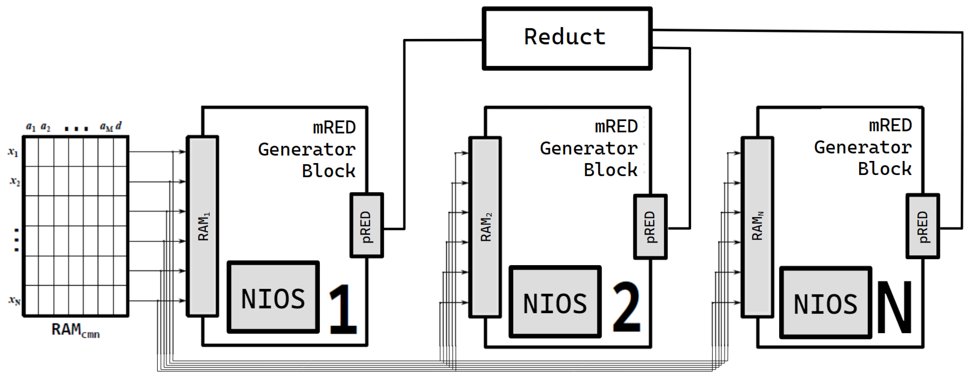
The FPGA serves as the core of the system, implementing the control logic, data flow coordination, and the mRED modules that perform parallel generation of parts of reducts. The overall FPGA-based system architecture is illustrated in Figure 1.

The system is composed of the following components:

• $RA{M}_{cmn}$—A memory block containing the portion of the decision table that is compared against the data segments stored in the individual $mRED$ Generator Blocks.
• $mRED$$GeneratorBlock$—A computational unit (described in detail later in this section) responsible for performing comparisons and calculations between two selected parts of the decision table.
• $NIOS$—An instantiated NIOS softcore processor responsible for coordinating data transfers between the main RAM and the shared memory module $RA{M}_{cmn}$.
• $RAM$$DecisionTable$—A representation of the decision table maintained in the primary RAM memory. Selected fragments of this table are forwarded to the shared memory $RA{M}_{cmn}$ under the control of the main NIOS processor, and subsequently distributed to the local memories of the $mRED$ blocks ($RA{M}_n$) by the internal NIOS processors embedded within each block.

The algorithm is executed by control software running on the NIOS II softcore processor. During each iteration of lines 6–22 of the REDUCT-MCPHIDM algorithm (see Section 2.3), the $RA{M}_{cmn}$ block is loaded with a segment of the decision table (line 7). Each $mRED$ block likewise stores its own designated segment of the table. A $mRED$ module computes attribute occurrence counts according to the procedure outlined in lines 10–20. When multiple instances of the $mRED$ block are instantiated, the operations corresponding to lines 10–20 can be replicated and executed concurrently, enabling substantial parallelism and reducing overall computation time.

3.2. Submodule Design

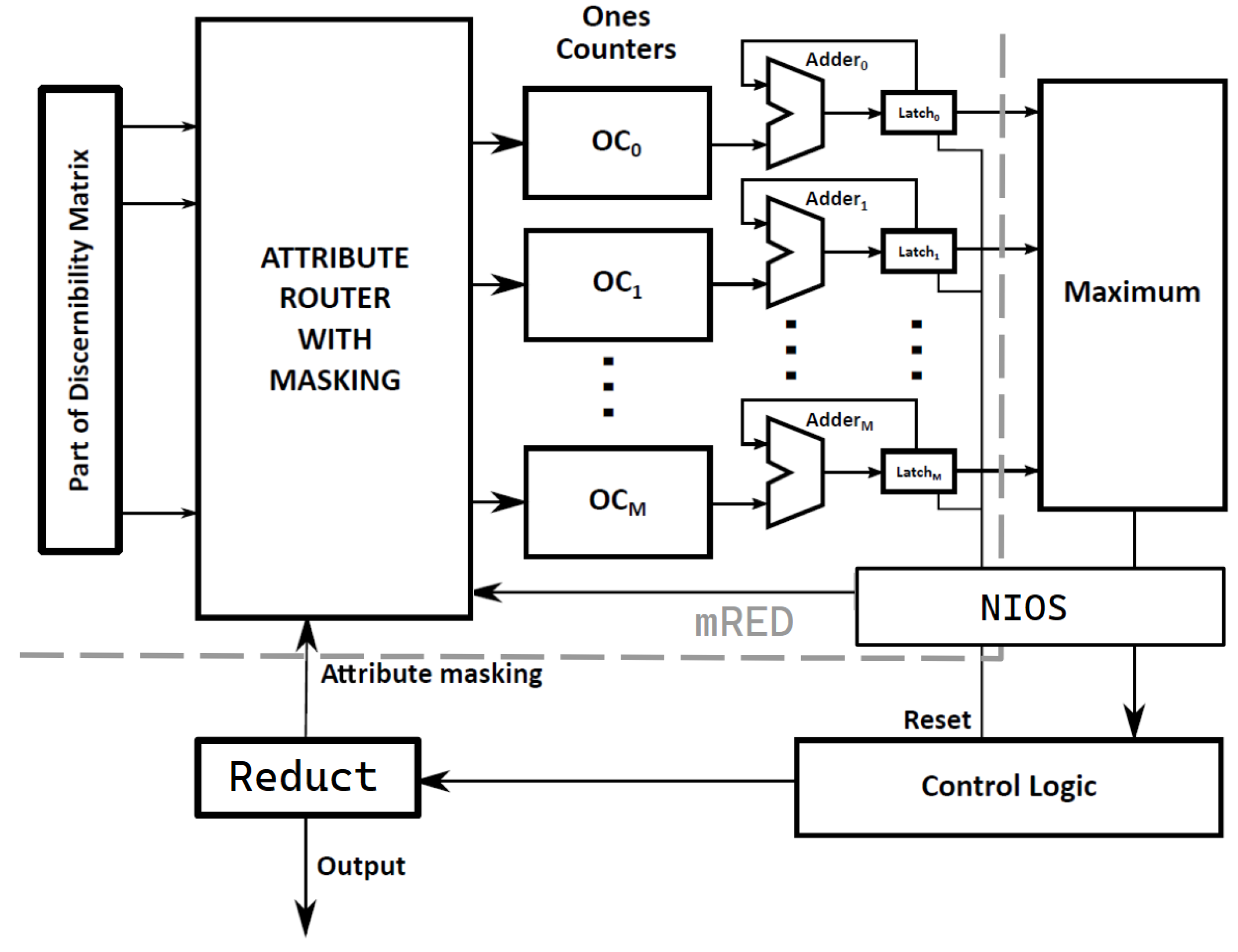
The REDUCT-MCPHIDM algorithm (Section 2.3) constructs a reduct using the discernibility matrix [2,3]. The hardware realization of these operations is encapsulated within the $mRED$ module. Its architecture, illustrated in Figure 2, is composed of the following elements:

• Attribute Router with Masking—A dedicated routing unit that distributes signals derived from the discernibility matrix to the ones counters. It supports attribute masking, enabling selected attributes to be excluded from processing. This behavior corresponds to the condition $a\in A\setminus R$ in line 23 of the algorithm.
• OC₀, …, OC_M—A set of ones counters, each responsible for counting the number of ‘1’ bits associated with a specific attribute in the discernibility matrix. Each $O{C}_i$ is assigned to exactly one attribute.
• Adder₀, …, Adder_M—Accumulation units that sum the counts returned by the ones counters, corresponding to the operation performed in line 15 of the algorithm. Every $Adde{r}_i$ is dedicated to a single attribute.
• Latch₀, …, Latch_M—Storage elements used to retain intermediate occurrence counts for each attribute. One $Latc{h}_i$ is provided per particular attribute.
• NIOS—A softcore processor tasked with coordinating data transfers from the main RAM, which stores fragments of the decision table, to the appropriate local memory $RA{M}_n$, as well as controlling the operation of the module’s control logic part.

Figure 2. Block diagram of the $mRED$ module.

Figure 2. Block diagram of the $mRED$ module.

The following components, also depicted in Figure 2, share inputs across all instantiated $mRED$ modules:

• Maximum—A module that identifies the attribute with the highest accumulated occurrence count.
• Control Logic—Module responsible for generating control signals, including attribute selection, latch reset after each computation cycle, and forwarding the most frequent attribute to the reduct block.
• Reduct—The register holding the final reduct produced by the system.

As each segment of the discernibility matrix is processed, the ones counters, together with the adders and latches, accumulate the total occurrence count for every attribute represented in the matrix. After all processing cycles have been completed, the maximum module shared among $mRED$ blocks identifies the attribute with the highest accumulated count. This information is provided to the control logic, which then forwards the selected attribute to the reduct register and subsequently marks it as ignored for the remaining iterations. When all attributes have been masked out, the content of the reduct register constitutes the final reduct, and the computation terminates.

Attribute selection and masking are executed within the Attribute Router with Masking (ARM) module. Each entry of the discernibility matrix is delivered to the ARM, where the relevant signals are provided depending on the attribute currently evaluated and subsequently processed by an AND-based masking stage. When the bit corresponding to an attribute is asserted in the Red register, the AND suppresses all matrix entries related to that attribute. The resulting masked outputs are then propagated to the ones counters, which handle the subsequent stages of computation.

3.3. Example of Operation

For clarity of presentation, only the most relevant data flow operations are illustrated, limited to a single partial iteration of the algorithm. The hardware processing unit requires the dataset to be transformed into a binary representation. An exemplary dataset after such transformation is shown in

Table 2. An exemplary binary dataset consisting of four condition attributes and one decision attribute.

ID	Outlook	Temp	Humidity	Windy	Mixing
1	1	1	1	0	0
2	1	1	1	1	0
3	0	1	1	0	1
4	1	0	1	0	1
5	1	1	0	0	1
6	1	1	0	1	0
7	0	1	0	1	1
8	1	0	1	0	0
9	1	1	0	0	1
10	1	0	0	0	1
11	1	0	0	1	1
12	0	0	1	1	1

.

The input values of the REDUCT-MCPHIDM RAM blocks are given as $RA{M}_1=RA{M}_2$ = 00111 01111 10110 10101 10011 01011 11010 00101 10011 10001 11001 11100. That data correspond to the exemplary binary decision table. The most significant bit (MSB) represents the decision attribute (mixing), whereas the least significant bit (LSB) corresponds to the outlook attribute.

The ARM module selects object $I{D}_1$ from $RA{M}_1$ represented by 00111 during the first clock cycle. This object is subsequently compared with all remaining objects stored in $RA{M}_2$ using the CB comparators. The resulting values correspond to the first column of the discernibility matrix constructed for the dataset. The binary word generated by the comparators is 0000 0000 0001 0010 0100 0000 1101 0000 0100 0110 1110 1011. The ones counters then determine the number of occurrences for each conditional attribute, defining the following outputs:

• $O{C}_0$—Value for outlook attribute is 3.
• $O{C}_1$—Value for temp attribute is 4.
• $O{C}_2$—Value for humidity attribute is 5.
• $O{C}_3$—Value for windy attribute is 3.

After each iteration, the result of the operation is forwarded to the adder blocks (equipped with latches) corresponding to each conditional attribute. Subsequently, all remaining objects are mutually compared. The values stored in the adders after completing the first main iteration (i.e., after comparing all 12 objects pairwise) are as follows:

• $Adde{r}_0$—Value for outlook attribute is 48.
• $Adde{r}_1$—Value for temp attribute is 64.
• $Adde{r}_2$—Value for humidity attribute is 72.
• $Adde{r}_3$—Value for windy attribute is 64.

The control logic evaluates the maximum block to identify the attribute with the highest occurrence. After the first main iteration, this corresponds to $Maximum2$ (associated with the humidity attribute), which has the value of 72. This attribute is then incorporated into the reduct RED by applying a logical OR operation to the current value of RED.

Next, the main loop proceeds to the subsequent attribute. According to the hardware algorithm described in Section 2.3, the following iteration is executed with previously selected attributes masked and excluded from further computations.

The final reduct obtained is $R=1111$, which corresponds to $R=\{outlook,temp,$$humidity,windy\}$.

4. Data and Experimental Results

This section presents the results of the experimental study, including descriptions of the data, methodology, the experimental conditions, and a discussion of the obtained results.

4.1. Data

This work employs three benchmark datasets: the Poker Hand [29], a medical dataset characterizing children diagnosed with insulin-dependent diabetes mellitus [30], and the Fashion Product Classification dataset [31].

The Poker Hand dataset, sourced from the UCI Machine Learning Repository [32], comprises 1,000,000 instances, each representing a five-card hand taken from a standard 52-card deck. Every card is specified by its suit and rank, resulting in ten conditional attributes per instance. Decision attribute identifies the resulting poker combination, covering ten classes arranged according to decreasing frequency: no combination, one pair, two pairs, three of a kind, straight, flush, full house, four of a kind, straight flush, and royal flush.

Type 1 diabetes mellitus is a chronic metabolic condition marked by impaired insulin production, requiring therapeutic insulin supplementation. The corresponding dataset contains 107 patient records, described by twelve conditional attributes, including physical examination findings and laboratory measurements, and one decision attribute representing the presence or absence of microalbuminuria. The original dataset is presented in [30], with an extended software-based evaluation provided in Chapter 6 of [3].

The Fashion Product Classification dataset, sourced from the Kaggle repository, comprises 44,446 instances, each representing a fashion product information including clothing categories, product types, colors, seasons, gender labels, and display names. Every object is specified by attributes named id, gender, masterCategory, subCategory, articleType, baseColour, season, year, usage, and productDisplayName. id and productDisplayName were used as identification attributes and usage was a decision attribute, resulting in seven conditional attributes per instance.

For experimental purposes, the Poker Hand dataset was downsampled to construct subsets of sizes between 1000 and 500,000 objects, while maintaining the original distribution of decision classes based on random selection of the objects. Conversely, the diabetes dataset was expanded to sizes between 1000 and 1,000,000 objects by replicating records from the source data by duplication of existing objects and sorting them randomly after extension to avoid creating repeatable data patterns. Similar rules were used for Fashion Product Classification dataset, both for downsampling and expansion.

All datasets for hardware implementation were subsequently converted into a binary format. For all datasets, each attribute value was coded using 4 bits. For the Fashion dataset, attributes subCategory and articleType used two 4-bit slots for coding its values. Consequently, each object occupied 44 bits in the Poker Hand dataset, 52 bits in the diabetes dataset, and 40 bits in the fashion dataset. To comply with FPGA memory alignment requirements, every object was padded to a 64-bit word by appending zero-valued bits.

4.2. Results

The software implementation of the REDUCT-MCPHIDM algorithm described in Section 2.3 was developed in the C programming language. It should be emphasized that the implementation utilized 1 to 4 CPU cores to provide a fair basis for comparison between the PC and FPGA solutions. The experiments were conducted on a workstation equipped with 32 GB of RAM and a 4-core Intel Core i7-1185G7 3.0 GHz processor, running Windows 11. The source code was compiled using the GNU GCC 12.1 compiler with the O2 compilation setting. High-computational parts of the software solution were implemented for parallel and multi-core excution using OpenMP 6.0 library.

Quartus II 13.1 was used for the compilation code in VHDL language. The synthesized solution was deployed on a Terasic DE-3 evaluation board containing a Stratix III EP3SL150F1152C2N FPGA device (Altera, San Jose, CA, USA). The FPGA operated at a 50 MHz clock frequency derived from the on-board oscillator, which was used for all sequential components of the design. The implemented REDUCT-MCPHIDM algorithm corresponds to the version presented in Section 2.3. A selected value of the FPGA clock frequency was used to ease the comparison between previous papers and the corresponding one.

The NIOS II softcore processor, together with the embedded-system peripherals, was generated using the Qsys 13.1 IDE. The accompanying NIOS II software was implemented in C and compiled via the NIOS II Software Build Tools for Eclipse.

Timing measurements were performed using a LeCroy WaveSurfer 104MXs-B oscilloscope (1 GHz BW, 10 GS/s sampling). For execution times that could not be measured by oscilloscope, on-chip hardware timers instantiated within the FPGA were employed. Each presented time result is the mean value of minimum 10 consequent runs of the solution on the same dataset. Relative standard deviation for measured run results did not exceeded 0.5% for hardware implementations and 2% for software solutions.

It should be noted that the PC clock frequency is approximately ${\displaystyle \frac{cl{k}_{PC}}{cl{k}_{FPGA}}}=60$ times higher than the FPGA system clock. It should be noted that this value represents only a theoretical algorithmic equivalence and is not a directly transposable practical advantage in all conditions, where the solution can adapted. Experiments were conducted using the datasets described in Section 4.1, with sizes ranging from 1000 to 1,000,000 objects. In every case, preprocessing (binary transformation and discretization) was performed on the PC.

Table 3. Execution time for both types of implementation for the REDUCT-MCPHIDM algorithm—one $mRED$ block and one CPU core.

Objects	${\mathit{t}}_{\mathit{H}}$	${\mathit{t}}_{{\mathit{S}}_1}$	$\mathit{C}=\frac{{\mathit{t}}_{{\mathit{S}}_1}}{{\mathit{t}}_{\mathit{H}}}$
—	[s]	[s]	—
Poker Hand dataset
1 k	0.051	0.527	10.310
2.5 k	0.217	2.727	12.578
5 k	0.926	11.327	12.237
10 k	3.483	43.922	12.609
25 k	20.584	271.724	13.201
50 k	79.121	1112.276	14.058
100 k	365.181	4477.226	12.260
250 k	2199.903	27,374.271	12.443
500 k	8504.588	110,877.710	13.037
1 M	31,088.792	402,407.110	12.944
Diabetes dataset
1 k	0.051	0.293	5.728
2.5 k	0.217	1.515	6.988
5 k	0.926	6.293	6.798
10 k	3.483	24.401	7.005
25 k	20.584	150.958	7.334
50 k	79.121	617.931	7.810
100 k	365.181	2487.348	6.811
250 k	2199.903	15,207.929	6.913
500 k	8504.588	61,598.728	7.243
1 M	31,088.792	223,559.505	7.191
Fashion dataset
1 k	0.051	0.234	4.582
2.5 k	0.217	1.212	5.590
5 k	0.926	5.034	5.439
10 k	3.483	19.521	5.604
25 k	20.584	120.766	5.867
50 k	79.121	494.345	6.248
100 k	365.181	1989.878	5.449
250 k	2199.903	12,166.343	5.530
500 k	8504.588	49,278.982	5.794
1 M	31,088.792	178,847.604	5.753

presents the execution times of the hardware ($t_H$) and software ($t_S$) implementations of the REDUCT-MCPHIDM algorithm for all datasets. The lower index in $t_S$ denotes the number of CPU cores used. The hardware solution in the first configuration employed a single instance of the $mRED$ generator block. Segments of the dataset were stored in $RA{M}_{cmn}$ and $RA{M}_1$. Software implementation used 1 CPU core for calculations.

The last columns of the tables show the acceleration factor for both types of implementation. The abbreviations used for dataset size are $k={10}^3$ and $M={10}^6$.

Table 4. Execution time for both types of implementation for the REDUCT-MCPHIDM algorithm—two $mRED$ blocks, as well as one and two CPU cores.

Objects	${\mathit{t}}_{\mathit{H}}$	${\mathit{t}}_{{\mathit{S}}_1}$	${\mathit{t}}_{{\mathit{S}}_2}$	${\mathit{C}}_1=\frac{{\mathit{t}}_{{\mathit{S}}_1}}{{\mathit{t}}_{\mathit{H}}}$	${\mathit{C}}_2=\frac{{\mathit{t}}_{{\mathit{S}}_2}}{{\mathit{t}}_{\mathit{H}}}$
—	[s]	[s]	[s]	—	—
Poker Hand dataset
1 k	0.027	0.527	0.293	19.877	11.061
2.5 k	0.112	2.727	1.518	24.251	13.495
5 k	0.480	11.327	6.304	23.593	13.129
10 k	1.807	43.922	24.442	24.309	13.528
25 k	10.676	271.724	151.210	25.451	14.163
50 k	41.038	1112.276	618.963	27.104	15.083
100 k	189.409	4477.226	2491.501	23.638	13.154
250 k	1141.028	27,374.271	15,233.317	23.991	13.351
500 k	4411.093	110,877.710	61,701.564	25.136	13.988
1 M	16,124.892	402,407.110	223,932.726	24.956	13.887
Diabetes dataset
1 k	0.027	0.293	0.169	11.043	6.368
2.5 k	0.112	1.515	0.874	13.473	7.770
5 k	0.480	6.293	3.629	13.107	7.559
10 k	1.807	24.401	14.072	13.505	7.788
25 k	10.676	150.958	87.058	14.139	8.154
50 k	41.038	617.931	356.362	15.058	8.684
100 k	189.409	2487.348	1434.457	13.132	7.573
250 k	1141.028	15,207.929	8770.432	13.328	7.686
500 k	4411.093	61,598.728	35,524.064	13.965	8.053
1 M	16,124.892	223,559.505	128,927.050	13.864	7.996
Fashion dataset
1 k	0.027	0.234	0.139	8.834	5.224
2.5 k	0.112	1.212	0.717	10.778	6.374
5 k	0.480	5.034	2.977	10.486	6.201
10 k	1.807	19.521	11.544	10.804	6.389
25 k	10.676	120.766	71.417	11.311	6.689
50 k	41.038	494.345	292.339	12.046	7.124
100 k	189.409	1989.878	1176.747	10.506	6.213
250 k	1141.028	12,166.343	7194.762	10.663	6.306
500 k	4411.093	49,278.982	29,141.917	11.172	6.607
1 M	16,124.892	178,847.604	105,764.402	11.091	6.559

presents the execution times for the hardware ($t_H$) and software ($t_{S_1}$ and $t_{S_2}$) implementations for the configuration, where the hardware system employs two instances of the $mRED$ module, while the software solution was executed on one and two CPU cores. The corresponding segments of the dataset are distributed across $RA{M}_{cmn}$, $RA{M}_1$, and $RA{M}_2$.

Table 5. Execution time for both types of implementation for the REDUCT-MCPHIDM algorithm—four $mRED$ blocks, as well as one and four CPU cores.

Objects	${\mathit{t}}_{\mathit{H}}$	${\mathit{t}}_{{\mathit{S}}_1}$	${\mathit{t}}_{{\mathit{S}}_4}$	${\mathit{C}}_1=\frac{{\mathit{t}}_{{\mathit{S}}_1}}{{\mathit{t}}_{\mathit{H}}}$	${\mathit{C}}_4=\frac{{\mathit{t}}_{{\mathit{S}}_4}}{{\mathit{t}}_{\mathit{H}}}$
—	[s]	[s]	[s]	—	—
Poker Hand dataset
1 k	0.014	0.527	0.163	38.323	11.868
2.5 k	0.058	2.727	0.844	46.755	14.479
5 k	0.249	11.327	3.508	45.487	14.086
10 k	0.937	43.922	13.601	46.868	14.514
25 k	5.538	271.724	84.146	49.069	15.195
50 k	21.285	1112.276	344.442	52.256	16.182
100 k	98.241	4477.226	1386.478	45.574	14.113
250 k	591.820	27,374.271	8477.083	46.254	14.324
500 k	2287.911	110,877.710	34,335.873	48.462	15.008
1 M	8363.533	402,407.110	124,614.762	48.114	14.900
Diabetes dataset
1 k	0.014	0.293	0.097	21.290	7.081
2.5 k	0.058	1.515	0.504	25.975	8.639
5 k	0.249	6.293	2.093	25.270	8.405
10 k	0.937	24.401	8.115	26.038	8.660
25 k	5.538	150.958	50.206	27.261	9.066
50 k	21.285	617.931	205.514	29.031	9.655
100 k	98.241	2487.348	827.253	25.319	8.421
250 k	591.820	15,207.929	5057.919	25.697	8.546
500 k	2287.911	61,598.728	20,486.773	26.924	8.954
1 M	8363.533	223,559.505	74,352.394	26.730	8.890
Fashion dataset
1 k	0.014	0.234	0.082	17.032	5.956
2.5 k	0.058	1.212	0.424	20.780	7.267
5 k	0.249	5.034	1.761	20.216	7.070
10 k	0.937	19.521	6.827	20.830	7.285
25 k	5.538	120.766	42.234	21.809	7.627
50 k	21.285	494.345	172.879	23.225	8.122
100 k	98.241	1989.878	695.888	20.255	7.083
250 k	591.820	12,166.343	4254.738	20.558	7.189
500 k	2287.911	49,278.982	17,233.541	21.539	7.532
1 M	8363.533	178,847.604	62,545.477	21.384	7.478

presents the execution times for the hardware ($t_H$) and software ($t_{S_1}$ and $t_{S_4}$) implementations for the configuration, where the hardware system utilizes four instances of the $mRED$ module, while the software solution was executed on one and four CPU cores. The corresponding dataset segments were stored in $RA{M}_{cmn}$, $RA{M}_1$, $RA{M}_2$, $RA{M}_3$, and $RA{M}_4$.

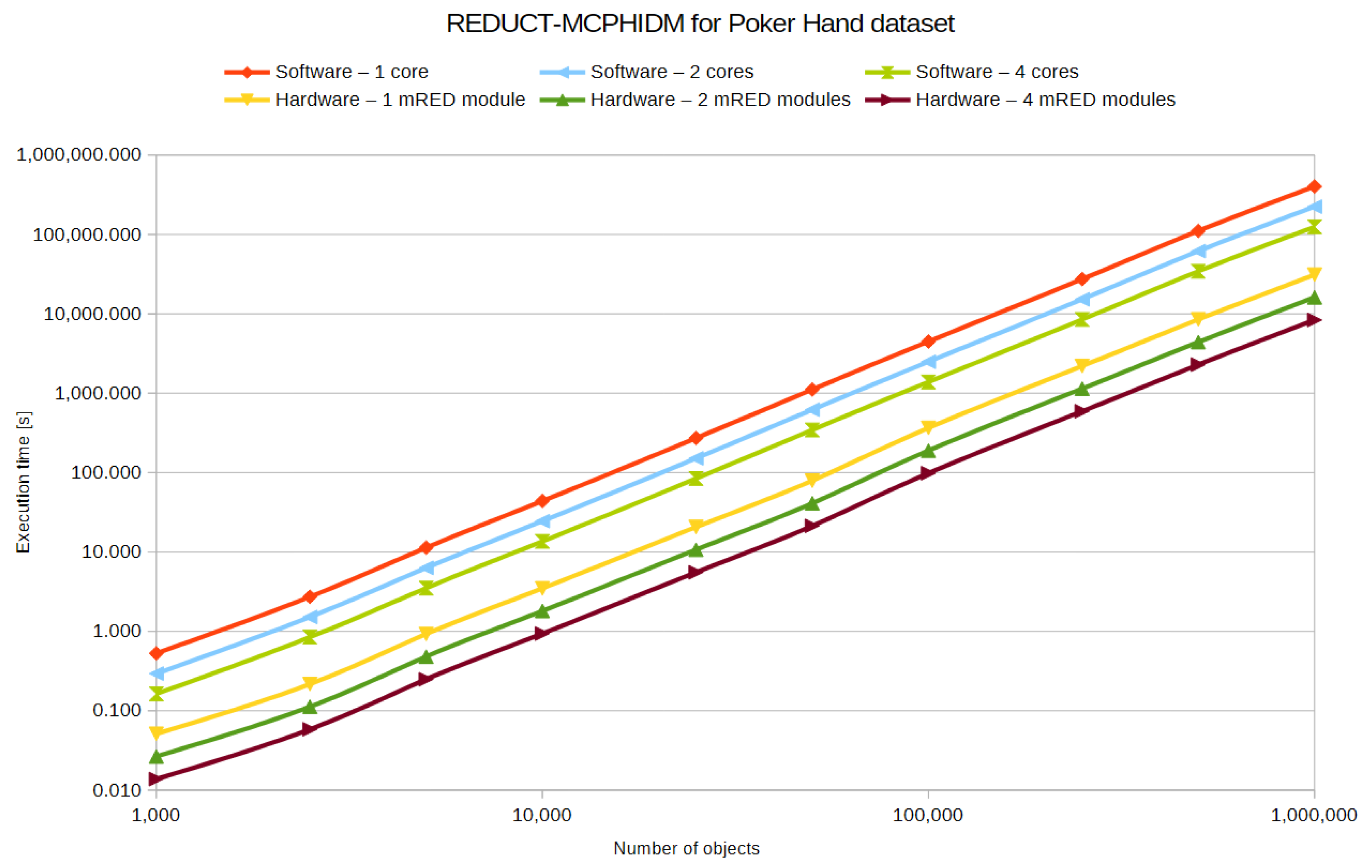
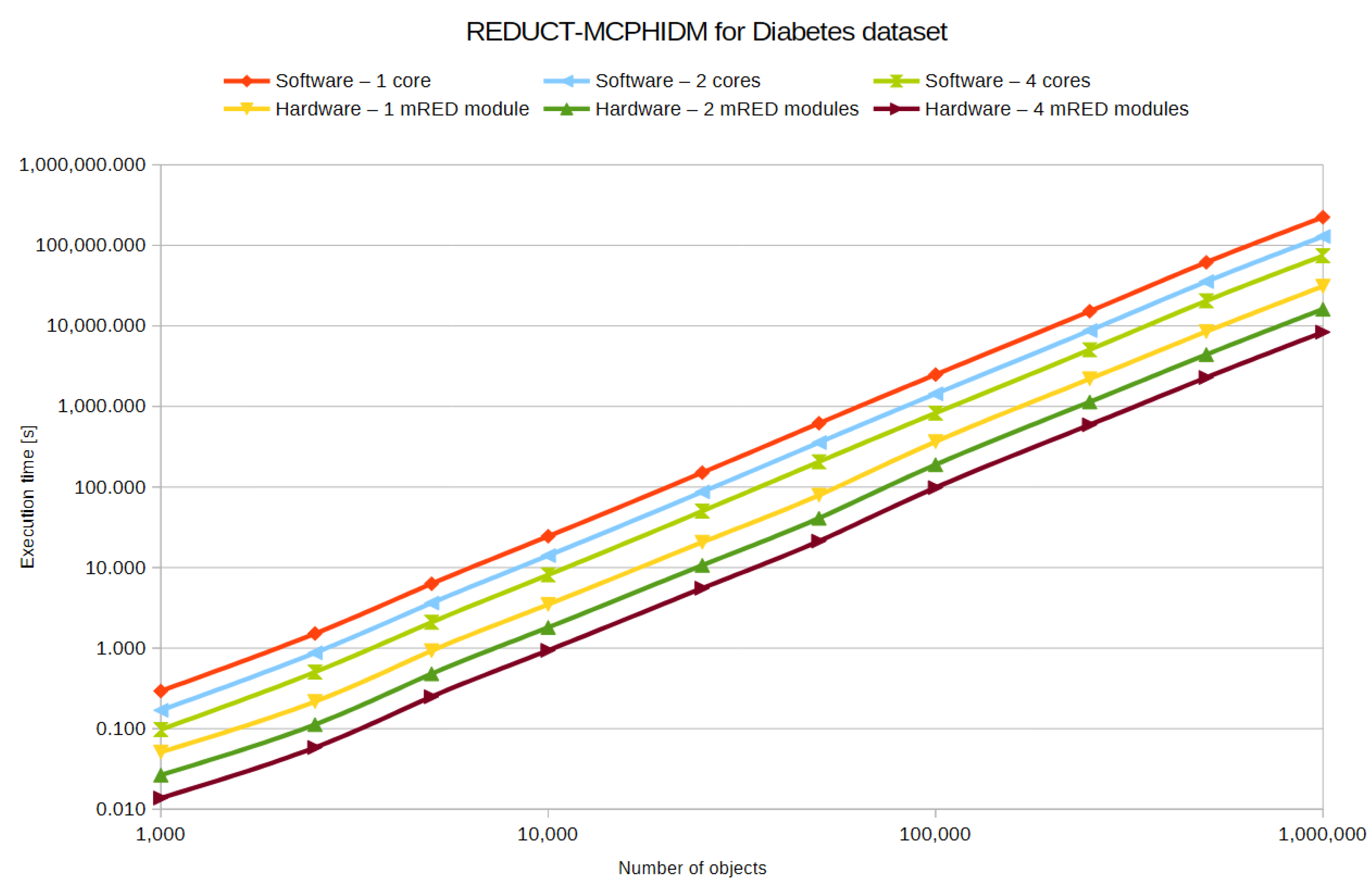
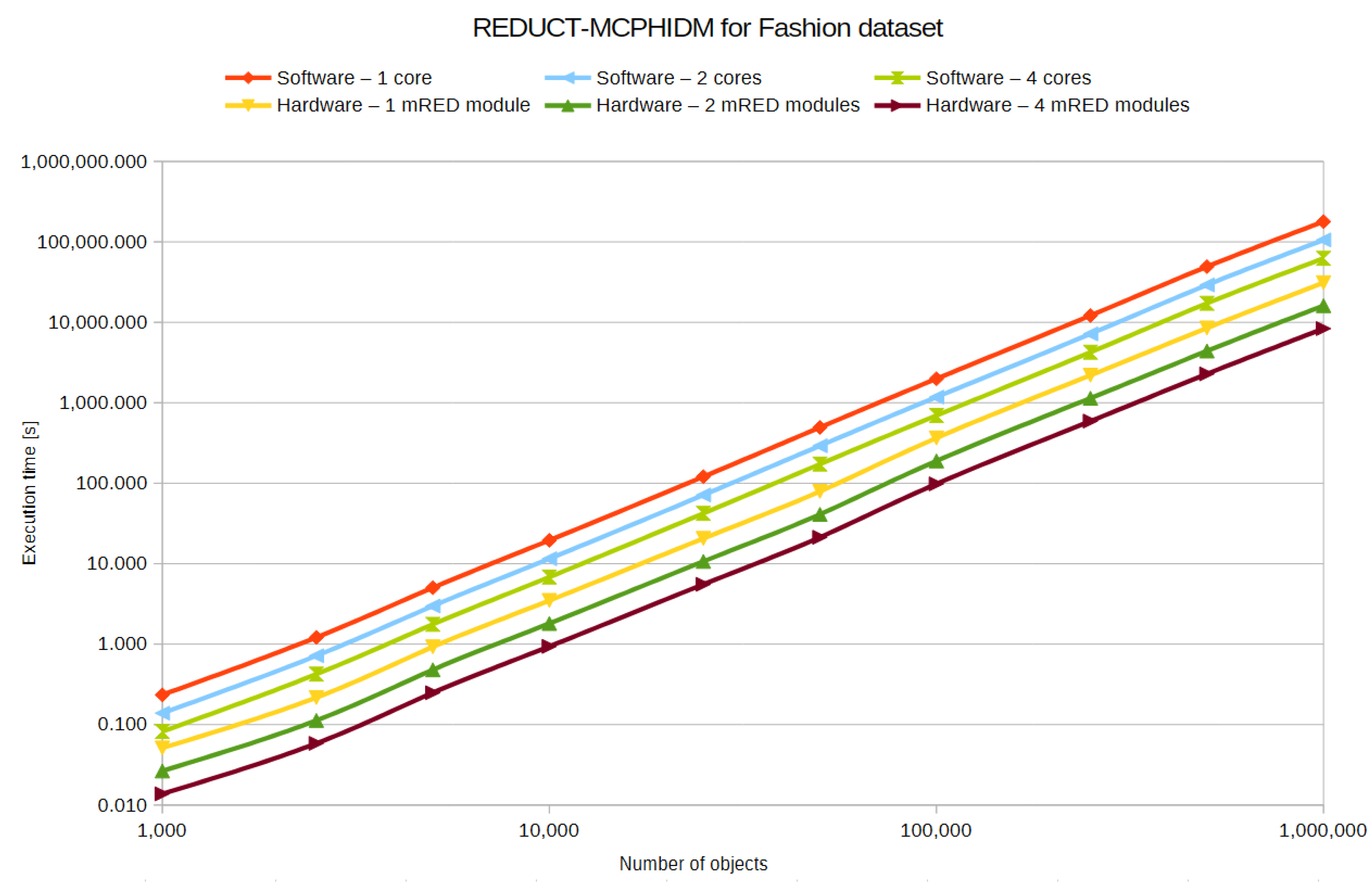
Figure 3, Figure 4 and Figure 5 show the relationship between the number of objects and the execution time for both types of implementation and configuration of $mRED$ modules, for the Poker Hand, Diabetes, and Fashion datasets respectively. Axes are presented on a logarithmic scale.

The presented results demonstrate a substantial improvement in data-processing performance across all evaluated configurations. When compared with the software implementation of the row-by-row discernibility matrix computation, the hardware execution achieves a speed-up of approximately 5 times when using a single $mRED$ module and up to 16 times when four $mRED$ modules are employed, compared with the same number of CPU cores used in software implementation. After accounting for the clock frequency difference between the PC and FPGA, the effective speed-up increases significantly. For a fixed hardware configuration used in the experiments, the speed-up remains nearly constant and is consistent across all evaluated dataset sizes.

The hardware processing times for all datasets are identical. The bit-width of individual objects does not influence execution time as long as it fits within the defined memory boundaries. Each hardware processing unit always operates on fixed-size 64-bit words and executes the same sequence of operations regardless of the dataset’s original attribute width. This holds for all configurations of the proposed reduct computation hardware modules.

The different hardware configurations and FPGA resource usage is presented in

Table 6. FPGA resource usage for different hardware configurations.

$\mathit{mRED}$ Blocks	Logical Elements (LE)	M9K	Max. Frequency	Max. Power
—	—	—	MHz	W
1	27,782	87	126	5.34
2	49,564	131	98	7.15
4	99,128	175	62	8.92

. The M9K column denotes the total number of M9K-type RAM blocks used, Max. frequency specifies maximum possible working frequency, while Max. power presents peak power consumption for a given configuration.

The average speed-up obtained by increasing the number of $mRED$ modules is not linear. The measured improvements are:

• 1.928 times for a solution with two $mRED$ blocks;
• 3.717 times for a solution with four $mRED$ blocks.

The reduction in scaling efficiency is primarily due to the overhead introduced by the NIOS II processors, which must copy binary data into the $RA{M}_n$ memories. It took around 3 to 6% of reduct calculation time. As the number of $mRED$ modules increases, this data transfer overhead becomes more significant, thereby reducing the overall speed-up. Measured data transfer times are presented in

Table 7. Data transfer times for REDUCT-MCPHIDM algorithm in different configurations.

Objects	1 mRED Module	2 mRED Modules	4 mRED Modules
—	[s]	[s]	[s]
1 k	0.002	0.001	0.001
2.5 k	0.007	0.005	0.003
5 k	0.028	0.022	0.015
10 k	0.105	0.081	0.056
25 k	0.618	0.480	0.332
50 k	2.374	1.847	1.277
100 k	10.955	8.523	5.894
250 k	65.997	51.346	35.509
500 k	255.138	198.499	137.275
1 M	932.664	725.620	501.812

. Columns for different number of mRED modules shows total time for data transfers and it can be noticed that reduction value is not linear with the number of modules because of increasing overhead related to data and results exchange.

The same situation for average speed-up factor can be noticed for the increasing number of CPU cores in software implementation. The average speed-up obtained by increasing the number cores is not linear and the measured values are:

• 1.691, 1.734, and 1.797 times for a solution with two CPU cores for the Fashion, Diabetes, and Poker Hand datasets respectively;
• 2.859, 3.007, and 3.229 times for a solution with four CPU cores for the Fashion, Diabetes, and Poker Hand datasets respectively.

The reduction in scaling efficiency is due to the implementation details related to the data path defined in parallel implementation. Parts of the decision table as well as intermediate results had to be copied to memory spaces used by different CPU cores. The difference in speed-up factor between both datasets is related to the number of conditional attributes as well as the data type used for encoding value of each attribute.

4.2.1. Solution Scalability

Expanding the horizontal size of the dataset (i.e., increasing the number of condition attributes) is possible; however, it requires enlarging the comparator structures in the DMGM module and increasing the width of the ones counters in the RGM and ARM modules. This is necessary because the system must process a wider binary word within the same clock cycle. Such modifications substantially increase FPGA resource requirements. In these cases, a larger FPGA device would be necessary, although modern high-capacity chips, such as the Intel Agilex I-Series 040 FPGA, which offers millions of logical elements, could satisfy these demands. As it was mentioned, the currently implemented design occupied 99,128 out of 113,600 available logic elements (approximately 87%) of the Intel Stratix III EP3SL340 device, leaving insufficient resources for a significantly larger number of modules while maintaining timing closure and routing feasibility. Therefore, the limit of four modules reflects the capabilities of the selected hardware platform rather than an inherent limitation of the proposed architecture. It should be noted that the proposed architecture is modular and scalable. Assuming theoretical approximate linear resource scaling, a single mRED module requires about 24,800 logic elements with additional resources for modules’ control logic, data, and results synchronization. Consequently, modern high-density FPGA devices could support substantially larger numbers of modules. For example, Intel Agilex devices offering 1–2.7 million logic elements could theoretically accommodate approximately 40–100 mRED modules, while comparable Xilinx Versal devices would provide a similar level of scalability. Practical factors such as routing congestion, data transfer overhead, and timing constraints will have a significant impact on those values, as it was presented in the previous paragraph with the discussion about speed-up factor decrease in correspondence with higher number of hardware modules.

4.2.2. Computational Complexity

The comparison of attribute values between two objects, as well as the retrieval of an element from the discernibility matrix, are considered elementary operations. Let m denote the number of conditional attributes and n the number of objects in the decision table. The computational complexity of the software-based implementation of reduct computation using the REDUCT-MCPHIDM algorithm is $\mathsf{\Theta }\left(m^2{n}^2\right)$. In contrast, the hardware implementation reduces the computational complexity to $\mathsf{\Theta }\left(m{n}^2\right)$. The elimination of one m results from the fact that the proposed solution enables simultaneous comparison of all attributes in constant time $\mathsf{\Theta }\left(1\right)$—the values of all attributes for a pair of objects are processed within a single clock cycle. Furthermore, the reduct computation module performs comparisons across multiple objects in parallel. Assuming that in typical applications $m<<n$, it can be concluded that the asymptotic computational complexity of both software and hardware approaches remains comparable.

5. Conclusions and Discussion

The conducted study confirms that implementing reduct computation directly in programmable hardware yields a substantial computational advantage over purely software-oriented approaches. The ability of FPGA to execute multiple operations concurrently, combined with their flexible architectural configuration, enables a significant reduction in processing time for large-scale decision tables. This positions hardware-based rough set processing as a viable foundation for high-performance decision-support solutions, particularly in scenarios where low latency or real-time operation is a critical requirement. Potential application areas include automated medical analysis, embedded intelligent controllers, security-oriented classification systems, and large-volume analytical workloads.

Despite the achieved performance improvements, the presented hardware architecture should be regarded as an intermediate step rather than a fully optimized solution. Several optimization opportunities remain open. Higher operating frequencies, as well as alternative clocking schemes such as dual-edge operation, could further shorten execution paths. Additionally, restructuring internal data paths through deeper pipelining and improved logic placement may significantly enhance throughput. The experimental results also indicate a strong positive scaling effect when multiple reduct units are instantiated in parallel. Given that most of the available resources of the Stratix III device are currently utilized, modern high-density FPGA platforms are expected to support a substantially larger number of parallel processing units, enabling efficient handling of big datasets.

Future investigations will therefore pursue multiple reinforcing directions. One objective is to analyze different architectural variants of the $mRED$ modules, focusing on trade-offs between resource consumption, timing limits, and computational efficiency. Furthermore, particular attention will be devoted to optimizing memory access patterns and communication channels between external memory, shared on-chip buffers, and computational units, as data transfer overhead remains a dominant performance factor with increasing number of module instances.

Future work will also extend the evaluation of the proposed approach by incorporating additional measures of reduct quality. In addition to computational performance, the analysis will include the number of attributes in the obtained reducts and the corresponding classification accuracy. This extended evaluation will allow for a more comprehensive assessment of the method, capturing both the efficiency of the reduction process and its effectiveness in preserving decision-making capability. In particular, combining reduct cardinality with classification performance will provide deeper insight into the trade-off between model compactness and predictive quality, enabling more complete validation of the proposed approach.

Equally important is the adaptation of the proposed hardware framework to more realistic data characteristics. At present, the system assumes fully specified decision tables without missing or ambiguous attribute values. However, real-world datasets, especially those derived from medical measurements, sensor networks, or sociotechnical systems, are often incomplete or affected by uncertainty. Since rough set methodology is inherently designed to operate under such conditions, extending the hardware architecture to support incomplete and noisy information systems constitutes a natural extension of this work. Achieving this goal would significantly broaden the applicability of the approach and further establish hardware-accelerated rough set analysis as a key component of future intelligent data-processing systems.

It should also be noted that some datasets, like Poker Hand, are characterized by a highly imbalanced distribution of decision classes, with the majority of objects belonging to a small number of dominant classes, while several classes are represented by only a limited number of instances. Since the REDUCT-MCPHIDM algorithm performs comparisons only between objects belonging to different decision classes, the number of generated object pairs depends directly on the class distribution. In highly imbalanced datasets, a large portion of comparisons involves objects from the dominant classes, whereas minority classes contribute relatively little to the total number of comparisons. Although class imbalance affects the absolute number of comparisons performed, it does not alter the computational structure of the algorithm. The speed-up factor is primarily determined by the degree of parallelization and hardware architecture rather than by the class distribution itself. However, class imbalance may slightly reduce the achievable parallel workload balance between processing units.

References

1. Marr, B.; Warren, J. Big Data: Principles and Best Practices of Scalable Real-Time Data Systems; Manning Publications: Greenwich, CT, USA, 2015. [Google Scholar]
2. Polkowski, L. Rough Sets, Rough Mereology and Uncertainty. In Thriving Rough Sets; Springer: Cham, Switzerland, 2017; pp. 49–85. [Google Scholar]
3. Stepaniuk, J. Rough-Granular Computing in Knowledge Discovery and Data Mining; Springer: Berlin/Heidelberg, Germany, 2008. [Google Scholar]
4. Chen, D.; Hu, Q.; Pedrycz, W. Multi-granulation rough sets for feature selection and attribute reduction. IEEE Trans. Fuzzy Syst. 2024, 32, 410–423. [Google Scholar] [CrossRef] [Scilit]
5. Zhang, J.; Liu, D.; Yao, Y. Incremental attribute reduction in dynamic decision systems based on generalized rough sets. Knowl.-Based Syst. 2024, 289, 111–128. [Google Scholar]
6. Liu, W.; Lu, K.; Lai, Z.; Li, S.; Ge, K.; Li, D.; Lu, X. AutoPipe-H: A Heterogeneity-Aware Data-Parallel Pipeline Approach on Commodity GPU Servers. IEEE Trans. Comput. 2025, 74, 1196–1209. [Google Scholar] [CrossRef] [Scilit]
7. Besozzi, V.; Della Bartola, M.; Dazzi, P.; Danelutto, M. High-Performance Serverless Computing: A Systematic Literature Review on Serverless for HPC, AI, and Big Data. IEEE Access 2025, 13, 195611–195656. [Google Scholar] [CrossRef] [Scilit]
8. Perepelitsyn, A.; Kulanov, V. Methods of Deployment and Evaluation of FPGA as a Service. Technologies 2025, 13, 266. [Google Scholar] [CrossRef] [Scilit]
9. Borowik, G.; Jankowski, J.; Kowalski, K. Fast algorithm for feature extraction. In Proceedings of the SPIE 9662, Photonics Applications in Astronomy, Communications, Industry, and High-Energy Physics Experiments; SPIE: Washington, DC, USA, 2015; pp. 1110–1117. [Google Scholar]
10. Zhang, J.; Wong, J.; Pan, Y.; Li, T. A parallel matrix-based method for computing approximations in incomplete information systems. IEEE Trans. Knowl. Data Eng. 2015, 27, 326–339. [Google Scholar] [CrossRef] [Scilit]
11. Geng, T.; Li, A.; Wang, T.; Wu, C.; Li, Y.; Shi, R.; Wu, W.; Herbordt, M. O3BNN-R: An Out-of-Order Architecture for High-Performance and Regularized BNN Inference. IEEE Trans. Parallel Distrib. Syst. 2021, 32, 199–213. [Google Scholar] [CrossRef] [Scilit]
12. Liang, Y.; Lu, L.; Xie, J. OMNI: A Framework for Integrating Hardware and Software Optimizations for Sparse CNNs. IEEE Trans. Comput.-Aided Des. Integr. Circuits Syst. 2020, 40, 1648–1661. [Google Scholar] [CrossRef] [Scilit]
13. Li, Z.N.; Zhu, C.; Gao, Y.L.; Wang, Z.K.; Wang, J. AlphaGo Policy Network: A DCNN Accelerator on FPGA. IEEE Access 2020, 8, 179676–179688. [Google Scholar] [CrossRef] [Scilit]
14. Pawlak, Z. Elementary rough set granules: Toward a rough set processor. In Rough-Neurocomputing: Techniques for Computing with Words; Springer: Berlin/Heidelberg, Germany, 2004; pp. 5–14. [Google Scholar]
15. Lewis, T.; Perkowski, M.; Jóźwiak, L. Learning in Hardware: Architecture and Implementation of an FPGA-Based Rough Set Machine. In Proceedings of EUROMICRO 1999; IEEE: Piscataway, NJ, USA, 1999; Volume 1, pp. 13–26. [Google Scholar]
16. Muraszkiewicz, M.; Rybiński, H. Towards a Parallel Rough Sets Computer. In Rough Sets, Fuzzy Sets and Knowledge Discovery; Springer: London, UK, 1994; pp. 434–443. [Google Scholar]
17. Kanasugi, A.; Yokoyama, A. A basic design for rough set processor. In Proceedings of the 15th Annual Conference of Japanese Society for Artificial Intelligence, Matsue, Japan, 22–25 May 2001. [Google Scholar]
18. Nguyen, S.H.; Nguyen, H.S. Some Efficient Algorithms for Rough Set Methods. In Proceedings of the Sixth International Conference on Information Processing and Management of Uncertainty in Knowledge-Based Systems (IPMU’96); Universidad de Granada: Granada, Spain, 1996; Volume III, pp. 1451–1456. [Google Scholar]
19. Narsale, N.; Agarwal, V. Implementation of LEM2 algorithm on FPGA. In Proceedings of ICECA 2019; IEEE: Piscataway, NJ, USA, 2019; pp. 1–5. [Google Scholar]
20. Tonde, S.; Agarwal, V. Implementation of lower and upper approximation features of rough set theory on FPGA. In ICCCNT 2021; IEEE: Piscataway, NJ, USA, 2021; pp. 1–5. [Google Scholar]
21. Tiwari, K.S.; Dattasamje, U.D.; Kadam, R.S.; Dudhedia, M.A.; Andhale, A.A.; Pansare, J.R.; Marlapalle, B.G. Design of exact reduct rough set hardware accelerator for early-stage diabetes risk prediction. Results Control Optim. 2024, 14, 100331. [Google Scholar] [CrossRef] [Scilit]
22. Hoozemans, J.; Peltenburg, J.; Nonnenmacher, F.; Hadnagy, A.; Al-Ars, Z.; Hofstee, H.P. FPGA Acceleration for Big Data Analytics: Challenges and Opportunities. IEEE Circuits Syst. Mag. 2022, 21, 30–47. [Google Scholar]
23. Molina, R.S.; Gil-Costa, V.; Crespo, M.L.; Ramponi, G. High-Level Synthesis Hardware Design for FPGA-Based Accelerators: Models, Methodologies, and Frameworks. IEEE Access 2022, 10, 90429–90455. [Google Scholar] [CrossRef] [Scilit]
24. Yan, F.; Koch, A.; Sinnen, O. A Survey on FPGA-Based Accelerator for ML Models. arXiv 2024, arXiv:2412.15666. [Google Scholar]
25. Kopczyński, M.; Grześ, T.; Stepaniuk, J. FPGA in Rough-Granular Computing: Reduct Generation. In Proceedings of the IEEE/WCI/ACM International Joint Conferences on Web Intelligence; IEEE: Piscataway, NJ, USA, 2014; Volume 2, pp. 364–370. [Google Scholar]
26. Kopczyński, M. FPGAs in Reduct Calculation Using Rough Sets. In Advances in Dependable Systems and Networks. DepCoS-RELCOMEX 2025; Lecture Notes in Networks and Systems; Springer: Cham, Switzerland, 2025; Volume 1427, pp. 96–105. [Google Scholar]
27. Kopczyński, M.; Grześ, T.; Stepaniuk, J. Computation of Cores in Big Datasets: An FPGA Approach. In International Conference on Rough Sets and Knowledge Technology; Lecture Notes in Computer Science; Springer: Cham, Switzerland, 2015; Volume 9436, pp. 153–163. [Google Scholar]
28. Kopczyński, M.; Grześ, T. FPGA supported rough set reduct calculation for big datasets. J. Intell. Inf. Syst. 2022, 59, 779–799. [Google Scholar] [CrossRef] [Scilit]
29. Cattral, R.; Oppacher, F.; Deugo, D. Evolutionary Data Mining with Automatic Rule Generalization. Recent Adv. Comput. Comput. Commun. 2002, 1, 296–300. [Google Scholar]
30. Stepaniuk, J. Knowledge discovery by application of rough set models. In Rough Set Methods and Applications; Physica-Verlag: Heidelberg, Germany, 2000; pp. 137–233. [Google Scholar]
31. Kaggle Homepage, Fashion Product Classification Dataset. Available online: https://www.kaggle.com/datasets (accessed on 23 June 2026).
32. Dua, D.; Graff, C. UCI Machine Learning Repository. University of California, Irvine, School of Information and Computer Sciences. 2017. Available online: https://archive.ics.uci.edu (accessed on 23 March 2026).
Figure 1. System overall architecture.
Applsci 16 07029 g001
Figure 3. Processing time in relation to input data size for Poker Hand dataset.
Applsci 16 07029 g003
Figure 4. Processing time in relation to input data size for Diabetes dataset.
Applsci 16 07029 g004
Figure 5. Processing time in relation to input data size for Fashion dataset.
Applsci 16 07029 g005