Analysis of Traction Performance for 180 HP Continuously Variable Transmission Tractor

Abstract

The traction performance analysis of hydro-mechanical transmission (HMT) tractors is employed to evaluate and optimize the transmission system during the design phase, thereby reducing research and development costs associated with continuously variable tractor transmission systems. However, there is currently no established methodological framework for calculating the traction performance of HMT tractors. To address this gap, this study integrated traditional tractor traction performance calculation equations with a self-developed HMT energy consumption calculation method, thereby developing a traction performance calculation model for HMT tractors. Initially, the principle of the tractor’s hydrostatic power-split transmission system was introduced. Subsequently, mathematical models for calculating transmission system energy consumption and tractor traction performance were established, with key sub-models experimentally validated to ensure the reliability of subsequent results. On this foundation, a calculation method for the traction performance of HMT tractors was proposed. Finally, models before and after energy consumption optimization, as well as models under different road conditions and transmission system configurations, were utilized as comparative models to calculate the traction performance of HMT tractors under various settings. The results indicate that energy optimization of HMT not only improves the transmission performance and reduces fuel consumption of HMT tractors, but also enhances the matching capability of HMT tractors with farm tools under high traction efficiency. Additionally, road conditions significantly impact the traction performance of HMT tractors. In wheat stubble fields, the tractor’s traction performance is substantially lower than on standard roads, with a maximum traction force decrease of 40.8% at a slip rate of 30%.

1. Introduction

The working environment of tractors is complex and variable, with significant randomness and time-varying characteristics in soil conditions, operational resistance, and load fluctuations, placing extremely high adaptability demands on the powertrain system of tractors. Hydro-mechanical transmission (HMT) is currently the most advanced tractor transmission system after power-shift transmissions [1,2]. It combines the high-load driving capability of hydraulic transmission with the low-energy consumption of mechanical transmission. In addition, it offers convenient operation and requires less time for operational adjustment, thereby significantly improving working efficiency. For a long time, the economy of tractors has been widely considered by engineers, so current research related to HMT mainly focuses on energy-saving design and control theory of the transmission system.

The economic performance of HMT is primarily determined by its energy consumption level, which is essentially characterized by its transmission efficiency [3]. In general, the transmission efficiency of HMT is related to the hydrostatic power portion, which is determined by its transmission principle [4]. When the engine power enters the HMT system, it is divided into two transmission paths. One part is transmitted to the planetary gear set through the swash-plate axial piston units (hydraulic path), while the other part is delivered to the planetary gear set through mechanical transmission (mechanical path). The power in the two paths converges in the planetary gear set and is output differentially. In this system, the transmission ratio of the mechanical path is fixed, while the transmission ratio of the hydraulic path can be continuously adjusted by changing the displacement ratio of pump to motor, thereby enabling the continuously variable speed regulation of HMT. When the displacement ratio is zero, all power is transmitted through a high-efficiency mechanical path, and HMT has the highest transmission efficiency. As the displacement ratio increases, the proportion of power flowing through the inefficient hydraulic path also increases, which consequently reduces the overall transmission efficiency of the HMT. Due to the above reasons, the full load efficiency curve of HMT shows a clear “hump” shape [5]. To improve efficiency, a common method is to adopt a multi-range technology to design the transmission. Specifically, the entire speed regulation range is divided into multiple ranges, thereby reducing the hydrostatic power flowing through each range. Without considering the rear axle, this scheme can generally achieve a full load efficiency of 80–90%, such as the Steyr S-Matic transmission with three power-split ranges. If the transmission design is fully optimized, the energy consumption of the transmission can be further reduced. For example, the CLAAS TRAXION transmission with five power-split ranges and the CLAAS HM8 transmission with seven power-split ranges achieve full load efficiencies of 88–93% and 89–94%, respectively [6]. Another method to improve HMT efficiency is to optimize the transmission system, which is a comprehensive approach that relies on mathematical modeling and is usually achieved through optimization algorithms. In this field, Zhou et al. [7] optimized a HMT with three cascaded standard planetary gear sets based on a particle swarm optimization (PSO) algorithm, aiming to reduce the hydrostatic power portion of the transmission and indirectly improve transmission efficiency. More research focuses on directly optimizing the efficiency of HMT. Xia et al. [8] used the NSGA-II algorithm to perform multi-objective optimization on the standing ratio of Simpson planetary gear set, which improved the tractor’s dynamic performance while achieving high HMT efficiency. Cheng et al. [9] also optimized the transmission parameters of HMT, but the goal was to maximize the efficiency of the tractor throughout its entire lifecycle. Li et al. [10] improved the efficiency of HMT by optimizing the configuration of the Simpson planetary gear set. The economy of HMT also depends on its matching control with the engine. Compared with mechanical transmissions, HMT generally exhibits higher energy consumption due to the presence of hydrostatic power. Renius [11] proposed a boundary efficiency curve, which states that only when the efficiency of HMT is consistently higher than the boundary curve, its energy consumption level is better than that of power-shift transmissions. In practice, except for a few transmissions such as Fendt Vario, most HMT systems struggle to meet this demanding technical requirement. However, this does not affect HMT becoming the most economical type of tractor transmission system. The same operating speed can be obtained by combining different engine speeds and transmission ratios, and different combinations correspond to different engine fuel consumption and different HMT efficiencies. Under certain control strategies, HMT can optimize engine speed and transmission ratio in real-time based on load conditions, ensuring that the powertrain always outputs power with minimum fuel consumption. This has been confirmed by numerous studies. Ince and Guler [12], as well as Wang et al. [13], compared the fuel efficiency between HMT and mechanical shift transmissions. D’Andrea et al. [14] investigated the fuel efficiency between HMT and hydrostatic transmissions, while Rossetti et al. [15] compared the fuel efficiency between HMT and power-shift transmissions. All research results indicate that HMT has the best fuel economy.

Although the energy consumption of HMT has attracted widespread attention, two important issues are often overlooked in existing research. Firstly, while HMT energy consumption can affect the transmission performance and fuel economy of tractors, it cannot be equated with the overall transmission performance and fuel economy of the entire tractor. Secondly, HMT energy-saving control strategies are primarily applied to light-load conditions with high fuel consumption. However, according to Renius’ research [11], tractors operate at speeds of 4–12 km/h for 68% of their lifecycle. At such low speeds, tractors mainly perform heavy-duty operations such as plowing and harrowing. Therefore, existing research not only ignores the overall power and fuel economy of tractors but also their typical operating conditions.

To fully evaluate HMT tractor performance during the design phase, avoid blind prototype manufacturing, reduce research and development costs, and improve research and development efficiency, it is necessary to analyze the tractor’s traction performance [16,17]. Traction performance refers to the comprehensive characteristics of power transmission, traction force utilization, and driving performance exhibited by the tractor during traction operations. It involves the coupling relationship of multidimensional parameters such as engine power output, transmission efficiency, wheel slip rate, hook traction force, driving speed, and fuel economy, directly reflecting the transmission performance and economy of the tractor under actual working conditions.

Currently, there is no established method system for calculating the traction performance of HMT tractors in this field. There may be two reasons: Firstly, as an advanced tractor transmission system, only a few enterprises possess HMT manufacturing capabilities. These enterprises typically keep their HMT system structures and parameters confidential, resulting in a lack of data required for HMT energy consumption calculations. Since HMT energy consumption is much more complex than that of traditional transmissions, this data gap hinders traction performance calculations. Secondly, current HMT energy consumption modeling often treats the power-split system as a closed transmission chain [18], with hydraulic system efficiency calculated separately [19]. This approach separates the coupling relationships between the hydraulic and mechanical systems, leading to low model accuracy. Such models are typically used only for qualitative comparisons, rather than for traction performance calculations.

Therefore, a high-reliable HMT energy consumption model is a necessary condition for studying tractor traction performance. Due to our team’s progress in HMT energy consumption calculation, this has created conditions for advancing related research. The contribution of this study is to propose a calculation model for HMT tractor traction performance, which fills the current research gap and enables analysis, comparison, and optimization of HMT tractor power and fuel economy during the design stage. This is crucial for reducing research costs associated with this expensive transmission system.

2. Materials and Methods

2.1. Transmission System

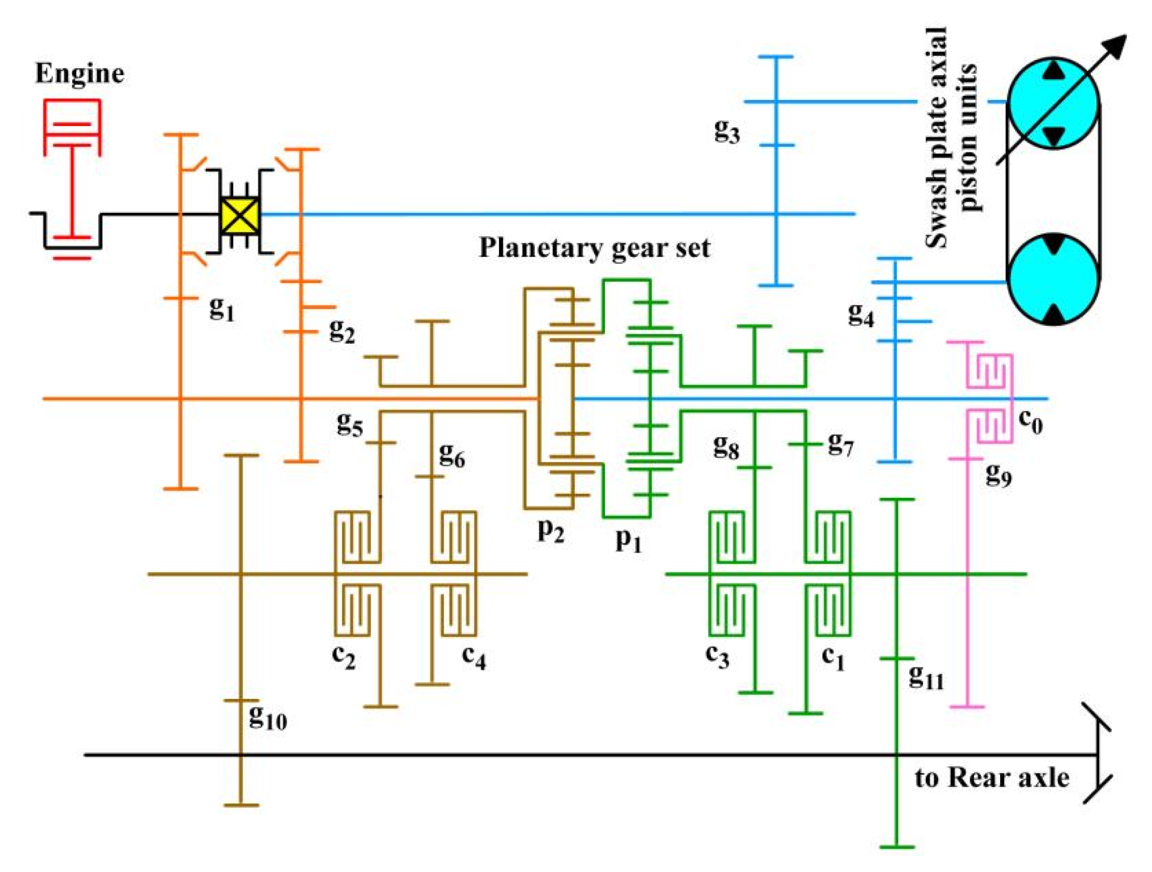
The HMT system of the 180 HP tractor is illustrated in Figure 1. After entering the transmission, the engine power is divided into a mechanical path and a hydrostatic path, both of which are then transmitted to the Simpson planetary gear set, where the power is combined and differentially output. The hydrostatic path consists of a closed hydraulic circuit composed of a variable-displacement pump and a fixed-displacement motor, and its transmission ratio varies with the displacement of the pump. In contrast, the transmission ratio of the mechanical path remains constant. The Simpson planetary gear set is formed by cascading two standard planetary gear sets, denoted as p₁ and p₂. When clutch c₁ or c₃ is engaged, planetary gear set p₁ transmits power, and the HMT operates in the power-split ranges HM₁ or HM₃. When clutch c₂ or c₄ is engaged, planetary gear set p₂ transmits power, and the HMT operates in the power-split ranges HM₂ or HM₄. The transmission ratios between HM₁ and HM₂, HM₂ and HM₃, and HM₃ and HM₄ are sequentially connected, enabling the tractor to achieve continuously variable speed regulation within the range of 4–50 km/h.

2.2. Energy Consumption Calculation

In the energy consumption calculation, the efficiency of the gears is assumed to be a constant value. Zhang et al. [20] and Zhou et al. [21] made the same assumption regarding gear meshing efficiency in the transmission system when investigating the traction performance of traditional tractors. Their experimental observations indicated that this assumption did not impact the accuracy of tractor traction performance predictions. However, the power calculations for the pump, motor, and planetary gear sets are relatively complex. Consequently, the energy consumption calculation methods for these components are introduced in detail.

2.2.1. Pump and Motor

The pump and motor form a closed hydraulic system and therefore satisfy the law of flow conservation. Considering leakage losses, the flow equation of the system can be expressed as follows:

$${\displaystyle \frac{\mathsf{\pi }{V}_{pmax}{n}_{p}e}{30}}={\displaystyle \frac{\mathsf{\pi }{V}_m{n}_m}{30}}+C_s∆p\left(V_{pmax}+V_m\right)/\mu$$

(1)

where $V_{pmax}$ and $V_m$ are the rated displacements of the variable-displacement pump and the fixed-displacement motor, respectively (m³/rad); $n_p$ and $n_m$ are the rotational speeds of the pump shaft and motor shaft, respectively, r/min; e is the actual displacement ratio of the pump to motor; $C_s$ is the total leakage coefficient; $∆p$ is the pressure difference between the inlet and outlet of the pump, Pa; and $\mu$ is the dynamic viscosity of the hydraulic oil, Pa·s.

Pumps and motors convert mechanical and hydraulic energy during operation. According to the law of energy conservation, the following equation can be obtained:

$$-∆p{V}_{pmax}e=-T_p+{\displaystyle \frac{f_p{n}_p\pi }{30}}-C_{fp}∆p{V}_{pmax}e$$

(2)

$$∆p{V}_m=T_m+{\displaystyle \frac{f_m{n}_m\pi }{30}}+C_{fm}∆p{V}_m$$

(3)

where $T_p$ and $T_m$ are the torques of the pump shaft and motor shaft, respectively N·m; $f_p$ and $f_m$ are the viscous damping coefficients of the pump shaft and motor shaft, respectively, N·m·s/rad; and $C_{fp}$ and $C_{fm}$ are the friction loss coefficients of the pump shaft and motor shaft, respectively.

2.2.2. Planetary Gear Set

The sun gear, ring gear, and planet carrier are the three fundamental components of a standard planetary gear set. Their rotational speed relationship can be expressed as follows:

$$n_s+k{n}_r-\left(1+k\right)n_c=0$$

(4)

where $n_s$, $n_r$, and $n_c$ are the rotational speeds of the sun gear, ring gear, and planet carrier, respectively, r/min; k is the standing ratio of the planetary gear set.

The torque relationship among the sun gear, ring gear, and planet carrier can be expressed as follows:

$$T_s+T_r+T_c=0$$

(5)

where $T_s$, $T_r$, and $T_c$ are the torques of the sun gear, ring gear, and planetary carrier, respectively, N·m.

In the conversion mechanism, when power flows from the sun gear to the ring gear, the torques of the fundamental components also satisfy the following relationship:

$$T_s=-T_c/\left(1+k{\eta }_{sr}\right)$$

(6)

or

$$T_s=T_r/\left(k{\eta }_{sr}\right)$$

(7)

where ${\eta }_{sr}$ is the meshing efficiency of the planetary gear set, which is numerically equal to the product of the meshing efficiency between the sun gear and the planet gear, and that between the planet gear and the ring gear.

Similarly, when power flows from the ring gear to the sun gear, the torques of the fundamental components satisfy the following relationship:

$$T_s=-T_c/\left(1+k{/\eta }_{sr}\right)$$

(8)

or

$$T_s=T_r/\left(k/{\eta }_{sr}\right)$$

(9)

For the ranges HM₁ and HM₃, the planet carrier of planetary gear set p₁ acts as the load end. Therefore, Equations (5), (6) and (8) are used to calculate the torques of the sun gear and ring gear. For the ranges HM₂ and HM₄, the ring gear of planetary gear set p₂ acts as the load end. Accordingly, Equations (5), (7) and (9) are used to calculate the torques of the sun gear and planet carrier.

In the above equations, the direction of power flow is determined by the relative rotational speed of the planet gear.

$$n_{pl}^c={\displaystyle \frac{\left(k{n}_r-n_s\right)}{\left(k-1\right)}}-n_c$$

(10)

where $n_{pl}^c$ is the relative rotational speed of the planetary gear, r/min.

When power flows from the sun gear to the ring gear, planetary gear set p₁ satisfies $n_{pl}^c\times T_c>0$, while planetary gear set p₂ satisfies $n_{pl}^c\times T_r<0$. Conversely, when power flows from the ring gear to the sun gear, planetary gear set p₁ satisfies $n_{pl}^c\times T_c<0$, and planetary gear set p₂ satisfies $n_{pl}^c\times T_r>0$.

2.2.3. Method Validation

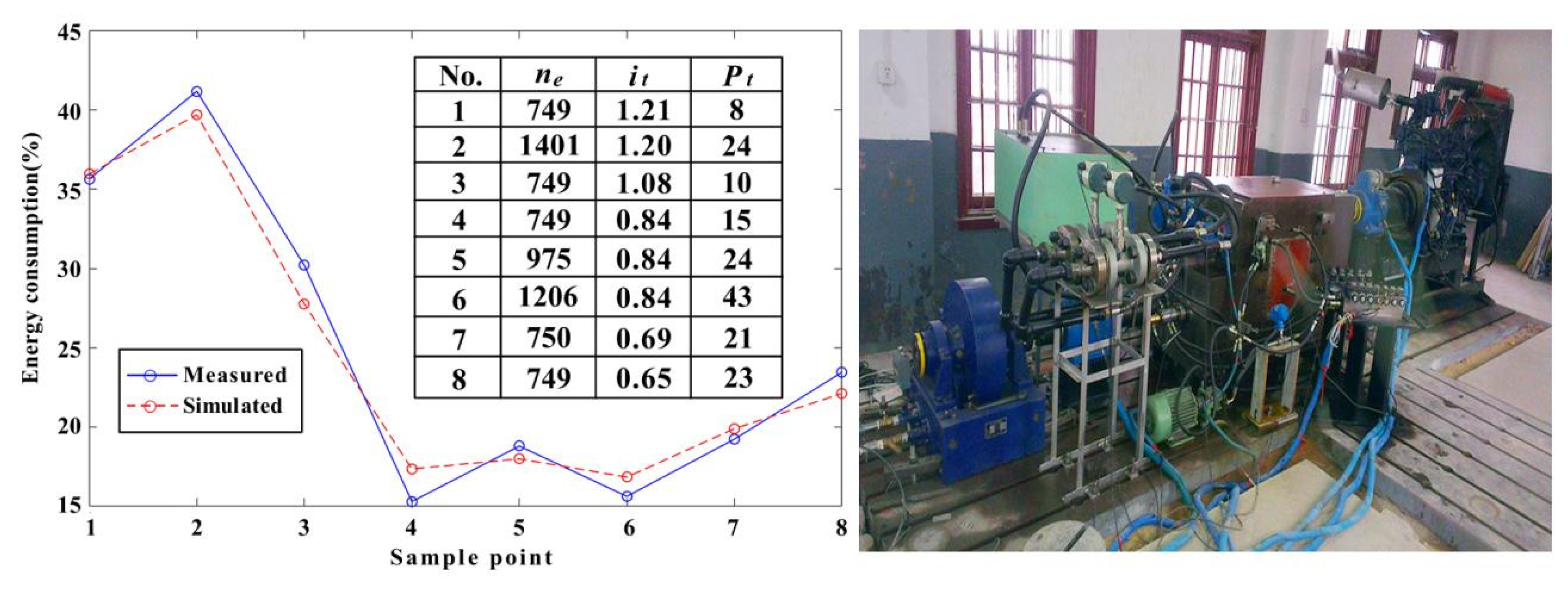
The energy consumption calculation method has been validated in our team’s previous research [13], and additional experimental results are provided to further demonstrate its reliability. The results are shown in Figure 2, where $n_e$ is the input speed of HMT, r/min; $i_t$ is the transmission ratio of HMT; and $P_t$ is the loading power of HMT, kW. As shown in the figure, the calculated energy consumption of the transmission closely matches the experimental results.

2.3. Traction Performance Calculation

The calculation of traction performance integrates the research conducted by Zhang et al. [20] and Zhou et al. [21]. These methods have been validated on the Taishan-25 tractor and the Dongfanghong-654 tractor, respectively. The specific derivation process is omitted here for brevity. The core equation is as follows:

The load borne by tractor tires is:

$$Z_2={\displaystyle \frac{\left(L-a+f_1{r}_1\right)G_s+F_t{h}_t}{L+f_1{r}_1-f_2{r}_2}}$$

(11)

$$Z_1=G_s-Z_2$$

(12)

where $Z_1$ and $Z_2$ are the vertical loads on the front and rear wheels of the tractor, respectively, m; L is the wheelbase of the tractor, m; $a$ is the distance from the tractor’s center of gravity to the rear axle, m; $f_1$ and $f_2$ are the rolling resistance coefficients of the front and rear wheels, respectively; $r_1$ and $r_2$ are the dynamic radii of the front and rear wheels, respectively, m; $G_s$ is the weight of the tractor, N; $F_t$ is the traction force of the tractor, N; and $h_t$ is the height of the traction hook, m.

The driving force equation of the tractor tires can be expressed as:

$$F_{q1}+F_{q2}=F_t+f_1{Z}_1+f_2{Z}_2$$

(13)

$$F_{q1}={\phi }_1{Z}_1$$

(14)

$$F_{q2}={\phi }_2{Z}_2$$

(15)

where $F_{q1}$ and $F_{q2}$ are the driving forces of the front and rear wheels, respectively; N; ${\phi }_1$ and ${\phi }_2$ are the driving force coefficients of the front and rear wheels, respectively.

When the tractor operates in four-wheel-drive mode, the speed coordination coefficient between the front and rear wheels is usually small, resulting in ${\phi }_1\approx {\phi }_2$. Therefore, ${\phi }_2$ can be directly calculated based on the traction force $F_t$. When the tractor operates in two-wheel-drive mode, ${\phi }_1=0$, and ${\phi }_2$ can also be directly obtained. Accordingly, the slip ratio of the rear driving wheels can be expressed as:

$$\delta ={\delta }^{\ast }\ln {\displaystyle \frac{{\phi }_{\mathrm{m}\mathrm{a}\mathrm{x}}}{{\phi }_{\mathrm{m}\mathrm{a}\mathrm{x}}-{\phi }_2}}$$

(16)

where δ and ${\delta }^{\ast }$ are the slip rate and the featured slip rate of the driving wheel, respectively; ${\phi }_{\mathrm{m}\mathrm{a}\mathrm{x}}$ is the maximum driving force coefficient of the rear driving wheels.

The actual travel speed of the tractor can be expressed as:

$$v=v^{\ast }\left(1-\delta \right)$$

(17)

where $v$ and $v^{\ast }$ are the actual travel speed and the theoretical travel speed of the tractor, respectively, km/h.

The traction power and the traction efficiency of the tractor can be expressed as:

$$N_t=F_{t}v/3600$$

(18)

$$\eta ={\displaystyle \frac{N_t}{N_e}}$$

(19)

where $N_t$ is the traction power, kW; $\eta$ is the traction efficiency; and $N_e$ is the engine power, kW.

The hourly fuel consumption and the specific fuel consumption of the tractor can be expressed as:

$$G_e=g_e{N}_e/1000$$

(20)

$$g_t=1000G_e/N_t$$

(21)

where $G_e$ is the hourly fuel consumption of the tractor, kg/h; $g_e$ and $g_t$ are the specific fuel consumption of the engine and the tractor, respectively, g/(kW·h).

2.4. Modeling

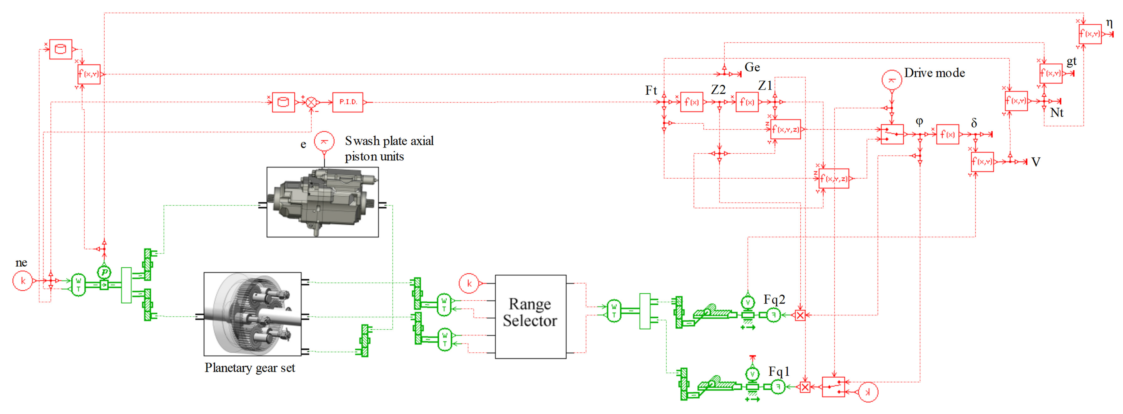
Based on the aforementioned equations, a model for calculating the traction performance of the HMT tractor was developed in AMESim (version 13.0.0), as illustrated in Figure 3. This model integrates energy consumption calculation with traction performance calculation, and its working principle is as follows:

(1)

Inputs determination: Based on the engine’s external characteristic curve and its speed regulation curve at full throttle, the target engine torque $T_e^{\ast }$ at a given engine speed $n_e$ can be interpolated. Other inputs include the transmission’s operating range, the displacement ratio $e$ of the pump to motor, and the drive mode (two-wheel drive or four-wheel drive).

(2)

Iterative calculation: Given the initial value of traction force $F_t$, the traction model calculates the driving force of each wheel based on the current driving mode, thereby loading the transmission system. The energy consumption model determines the transmission route according to the current HMT range and displacement ratio $e$, and calculates the actual engine torque $T_e$ step by step. The PID module adjusts the traction force $F_t$ based on the error $\Delta \epsilon$ between $T_e^{\ast }$ and $T_e$ until $\Delta \epsilon \approx 0$. After the model converges, traction performance data, including traction force, are recorded.

(3)

Termination condition: Starting from the maximum engine speed, gradually reduce the engine speed thereafter to obtain the tractor traction performance at any engine speed. The calculation terminates once the slip rate exceeds the preset threshold (such as 50%) or the engine speed has dropped to the value corresponding to its maximum torque (i.e., 1500 r/min).

During the calculation process, the engine considered is a Weichai WP6T180E21 diesel engine (Weichai Power Co., Ltd., Weifang, China), the HMT is a prototype transmission independently developed by our research team, and the tractor is based on a mainstream model of 180 hp tractors produced in China. The calculation parameters for traction performance are shown in

Table 1. Calculation parameters for tractor traction performance.

$\mathit{L}$ (m)	$\mathit{a}$ (m)	${\mathit{r}}_1$ (m)	${\mathit{r}}_2$ (m)	${\mathit{G}}_{\mathit{s}}$ (N)	${\mathit{h}}_{\mathit{t}}$ (m)
2.760	1.035	0.595	0.85	83,300	0.465

. Considering that tractors operate within the speed range of 4–12 km/h for 68% of their service life [11], this study focuses only on the transmission ranges HM1 and HM2, which correspond to a tractor speed range of approximately 4–15 km/h at rated input speed. Note that this model is constructed based on deterministic equations; thus, it is platform-independent, and completely consistent calculation results can be obtained using any simulation software (such as Matlab/Simulink). However, the batch processing function of AMESim can significantly improve calculation efficiency.

It is noted that the industrialization of HMT tractors in China is in its early stages, and the limited number of existing products have not disclosed their transmission system structures and parameters, rendering them unsuitable for traction performance research. The HMT developed herein features a validated energy consumption model but has not yet been assembled into a complete tractor. While it possesses the necessary modeling conditions for traction performance analysis, experimental verification of the final model cannot be conducted. However, the equations employed for traction performance calculations have been experimentally validated by Zhang et al. [20] and Zhou et al. [21]. Compared to their research, this study differs in two aspects: first, the traditional gearbox energy consumption model is replaced by the HMT energy consumption model, which has been experimentally validated; second, real engine test data are used in place of the engine model from their study, which is expected to further enhance computational accuracy. Therefore, this study can be considered reliable. Additionally, the objective of this study is to evaluate, compare, and optimize the performance of different HMT configurations during the transmission design phase, with the aim of reducing high research and development costs associated with blind trial production of HMT tractors. The current model is sufficiently capable of meeting the requirements for engineering applications, and there is no need to pursue high-precision performance prediction results as the research objective.

2.5. Comparison Model

To conduct a comparative analysis of the traction performance of the HMT tractor, two comparison models are proposed in this study: one optimized for energy consumption and the other considering different road conditions.

(1)

Energy consumption optimization

Previous research by our team has demonstrated that the transmission ratio of the gear pair ahead of the pump has a direct impact on the efficiency of the HMT under speed constraints [13]. The transmission ratio of this gear pair in the experimental prototype is 0.678. Increasing the transmission ratio to reduce the pump shaft speed can yield two beneficial effects: first, the viscous damping losses associated with speed in the hydraulic system decrease as input speed diminishes; secondly, under the same hydrostatic power portion, lower speeds correspond to higher torque, enabling the hydraulic system to operate in a low-flow, high-pressure state and significantly reducing flow losses. However, the pump shaft speed cannot be reduced indefinitely, as excessively low speeds may cause the pressure to exceed the continuous operating pressure limit of the closed system. According to research findings, when the transmission ratio of the gear pair ahead of the pump is set to 1, the energy consumption of the HMT reaches its optimal level.

(2)

Road condition

The rolling resistance coefficient, featured slip rate, and driving force coefficient of tractors vary under different road conditions. In this study, two types of road conditions will be discussed [20]: one is the traction test road of the Luoyang Tractor Research Institute (standard road), with a rolling resistance coefficient close to 0.03, and the values of ${\delta }^{\ast }$ and ${\phi }_{\max }$ are approximately 0.092 and 0.995, respectively; the other is the wheat stubble field in northern China, with an average rolling resistance coefficient of 0.06 under suitable cultivation humidity, and the values of ${\delta }^{\ast }$ and ${\phi }_{\max }$ are approximately 0.15 and 0.704, respectively.

(3)

Commercial HMT

The HMT described in this study is classified as a Simpson configuration. To investigate the effect of HMT configuration on traction performance, this study compares the Simpson HMT with the New Holland 2-range tractor HMT based on the 2Z-X (B) configuration. To ensure a fair comparison, the rear axle parameters of the New Holland tractor were adjusted, and the tires used in this study were employed to ensure that all tractors had the same speed range.

2.6. Scientific Contribution and Novelty

The novelty of this study lies in the proposal of a traction performance calculation model for HMT tractors. The model comprises two components: an energy consumption model for HMT tractors, which we have proposed and experimentally validated, and a traction performance calculation model that references equations from previous studies. Zhang et al. [20] and Zhou et al. [21] were the first to construct traction performance calculation programs for tractors based on these equations. However, these computer programs, developed over 30 years ago, rely on clear causal relationships and are unable to exchange data with our HMT energy consumption model, as the latter can only be solved through iterative calculations. Consequently, we employed a completely different methodology to integrate and reconstruct the traction performance calculation model for HMT tractors. In other words, while some of our research and previous studies on traditional tractors were constructed using the same equations, they utilized different calculation methods. Our contribution is to further expand research on HMT energy consumption, enabling analysis and optimization of tractor performance from the perspectives of vehicle power and fuel economy, rather than being limited to the energy consumption of the transmission system itself.

3. Results and Discussion

3.1. Analysis of Calculation Results Under Standard Road Conditions

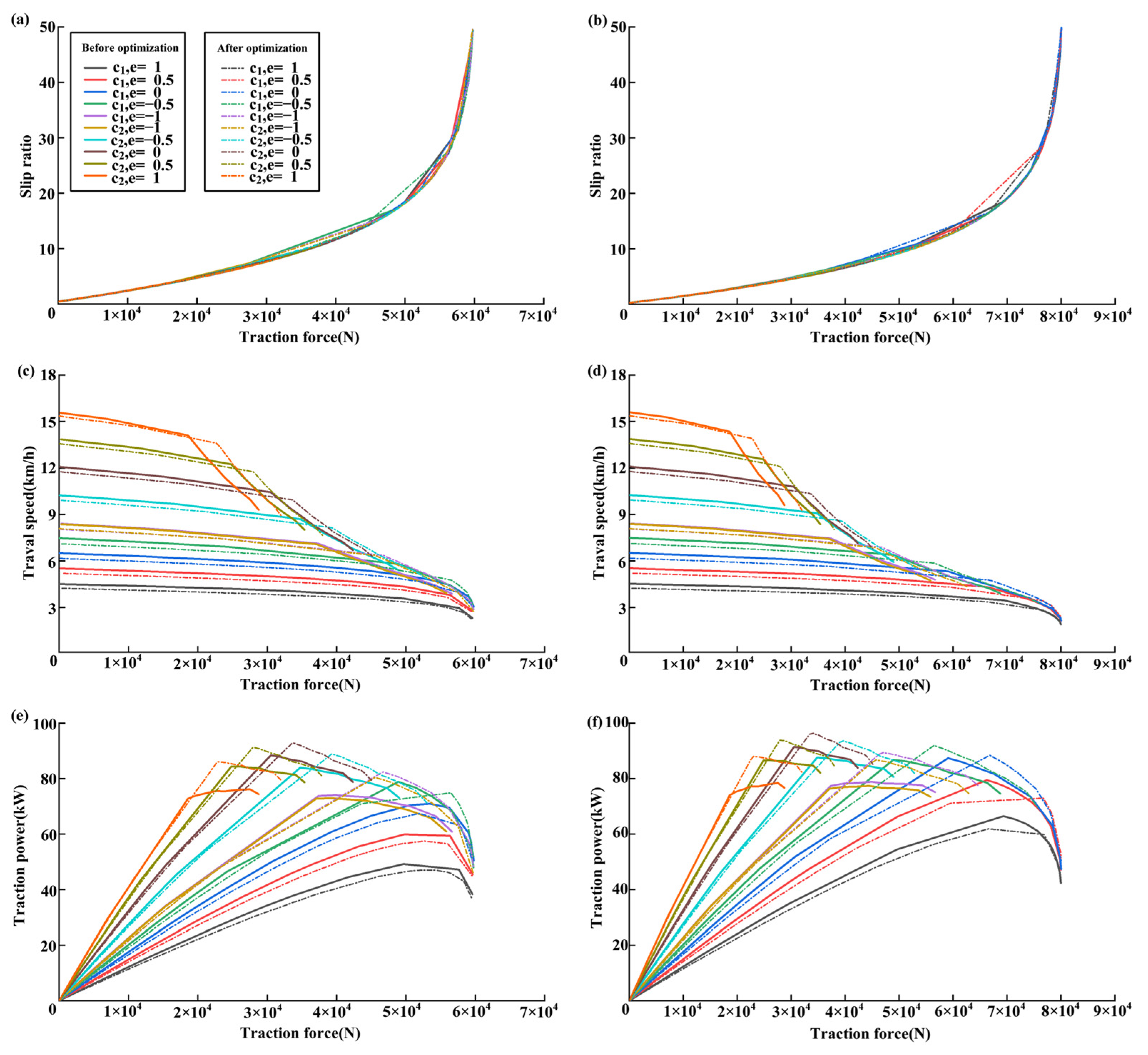
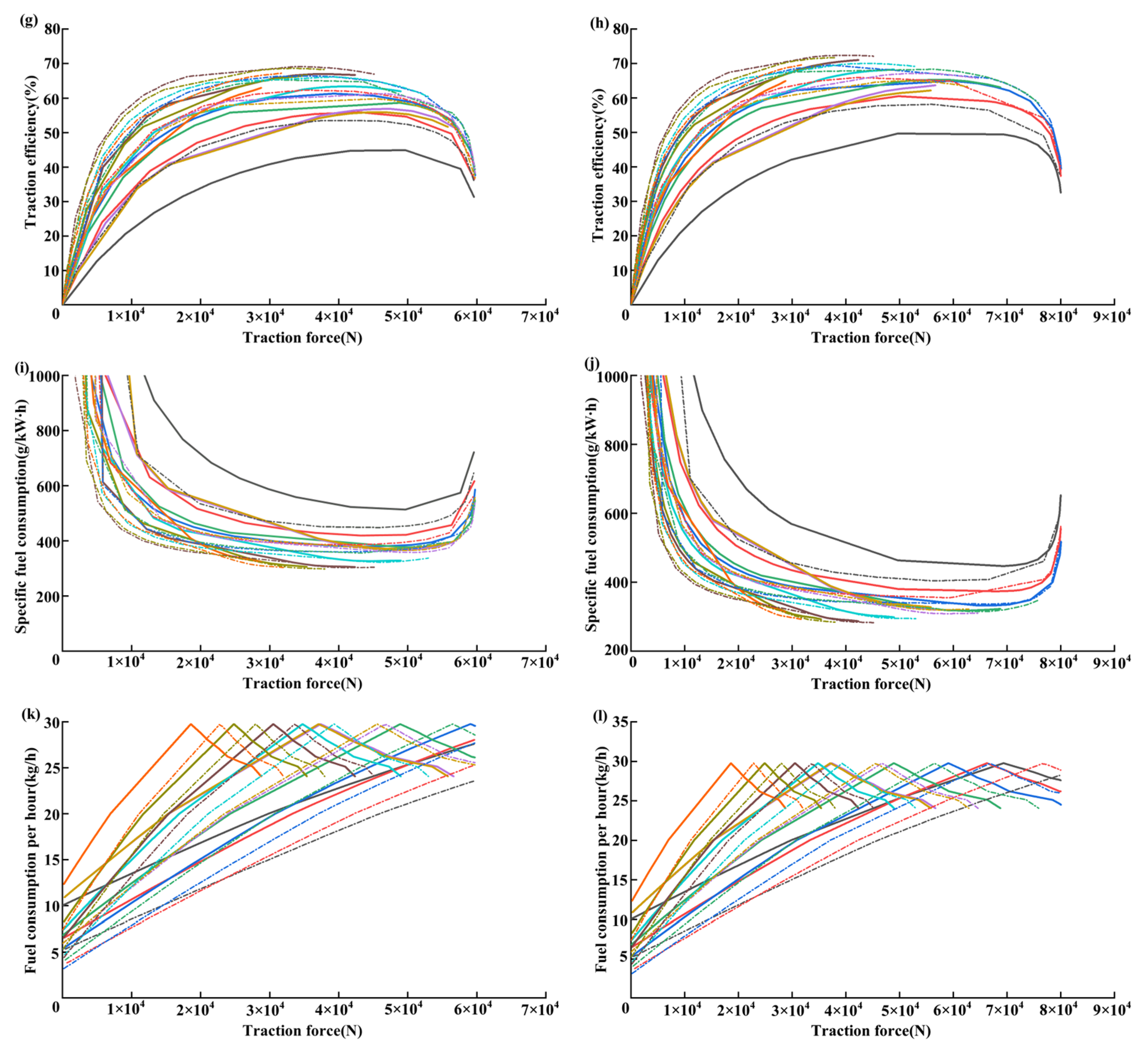
The comparison of traction performance of the HMT tractor before and after energy consumption optimization on standard road conditions is shown in Figure 4. It can be observed that:

(1)

Speed characteristics of the tractor: ➀ The energy consumption optimization of the HMT has little effect on the slip ratio curve. ➁ The energy consumption optimization of the HMT can significantly enhance the maximum traction force of the tractor at speed inflection points, making it less prone to slipping. This trend becomes more pronounced as the tractor speed increases. Taking the range HM2, $e=1$, and four-wheel-drive mode an example, the traction force of the tractor at speed inflection point increases from 18.58 kN before optimization to 22.79 kN, an increase of 22.66%.

(2)

Power characteristics of the tractor: ➀ The energy consumption optimization of the HMT has significantly improved the maximum traction power of the tractor, and this trend becomes even more pronounced as the tractor speed increases. Taking the range HM2, $e=0$, and four-wheel-drive mode as an example, the maximum traction power of the tractor increases from 91.46 kW before optimization to 96.72 kW, an increase of 5.75%. ➁ The energy consumption optimization of the HMT has comprehensively improved the traction efficiency of the tractor, which is significant at all tractor speeds, especially at low speeds. Taking the range HM1, $e=1$, and four-wheel-drive mode as an example, the maximum traction efficiency of the tractor increases from 50.72% before optimization to 58.22%, an increase of 14.79%. It is noted that this beneficial effect is not limited to specific operating conditions, but occurs at almost all levels of traction force.

(3)

Fuel consumption characteristics of the tractor: ➀ The energy consumption optimization of the HMT significantly reduces the specific fuel consumption of the tractor, which is most pronounced during low-speed operations. This means that tractors can achieve superior fuel economy through energy consumption optimization during low-speed and heavy-load operations such as plowing. Taking the range HM1, $e=1$, and four-wheel-drive mode as an example, the minimum specific fuel consumption of the tractor decreases from 442.92 g/(kW·h) before optimization to 403.45 g/(kW·h), resulting in an 8.91% fuel saving. Similarly, this beneficial effect covers almost all traction force levels. ➁ Under the same traction force, HMT can achieve lower hourly fuel consumption after energy consumption optimization, and this pattern applies to all tractor speed levels. Taking the range HM2, $e=1$, and four-wheel-drive mode as an example, the energy consumption optimization reduces hourly fuel consumption by approximately 3.48 kg/h at almost all traction force levels.

(4)

Impact of drive mode: ➀ The impact of energy consumption optimization on the traction performance of the tractor is reflected in all drive modes and follows a consistent pattern. ➁ The traction performance of the tractor in four-wheel-drive mode is generally higher than that in two-wheel-drive mode, which is consistent with common sense. Taking the speed characteristics at a slip rate of 10% as an example, the maximum traction forces of the HMT tractor in two-wheel and four-wheel-drive modes are 36.3 kN and 52.4 kN respectively, with the latter showing a 44.4% increase compared to the former.

The fundamental reason for enhancing traction performance through energy consumption optimization is to reduce engine power losses within the HMT. This allows a greater proportion of power to be allocated to traction operations, which is critical for improving both traction power and efficiency. Additionally, this improvement contributes to reduced tractor fuel consumption. For example, at the maximum traction power point, which corresponds to the engine’s rated power point (2200 r/min, 132.5 kW), engine fuel consumption at this operating condition is fixed. While improvements in traction efficiency do not alter the hourly fuel consumption rate, they inevitably lower the tractor’s specific fuel consumption by increasing the amount of useful work output.

3.2. Analysis of Calculation Results on Wheat Stubble Fields

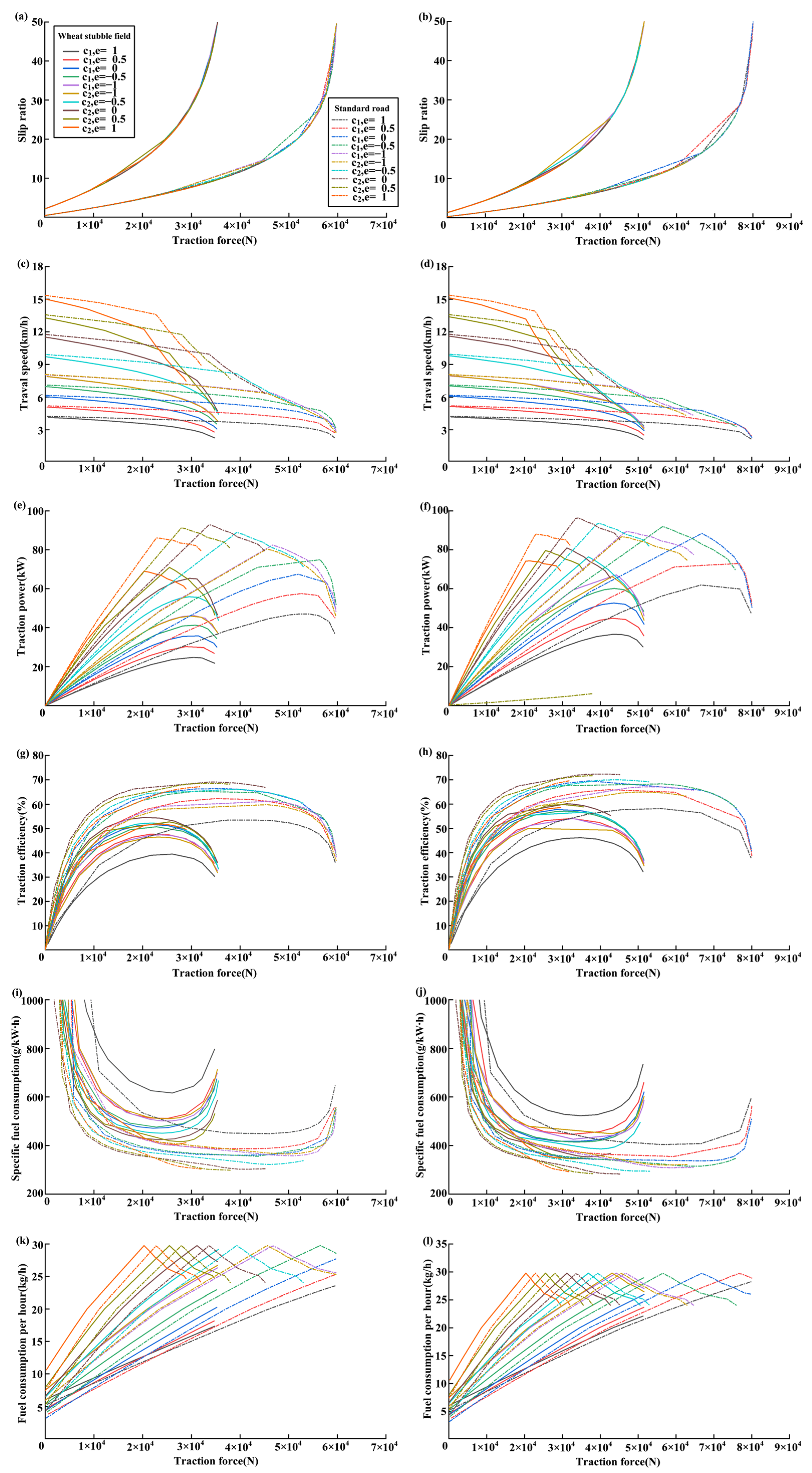
The comparison of traction performance of the energy consumption optimized HMT tractor on wheat stubble fields and standard roads is shown in Figure 5. It can be seen that the tractor is more prone to slipping when operating on wheat stubble fields, and the available traction force at the same slip ratio is lower than that on standard roads. Taking a slip ratio of 30% and the four-wheel-drive mode as an example, the maximum traction forces on the standard road and wheat stubble field are 77.2 kN and 45.7 kN, respectively, with the latter being 40.8% lower than the former. In addition to the speed characteristics, the power and fuel consumption characteristics of the tractor on wheat stubble fields also show a corresponding decrease. The above-mentioned pattern also applies to both two-wheel-drive and four-wheel-drive modes.

3.3. Analysis of Calculation Results on New Holland Tractor

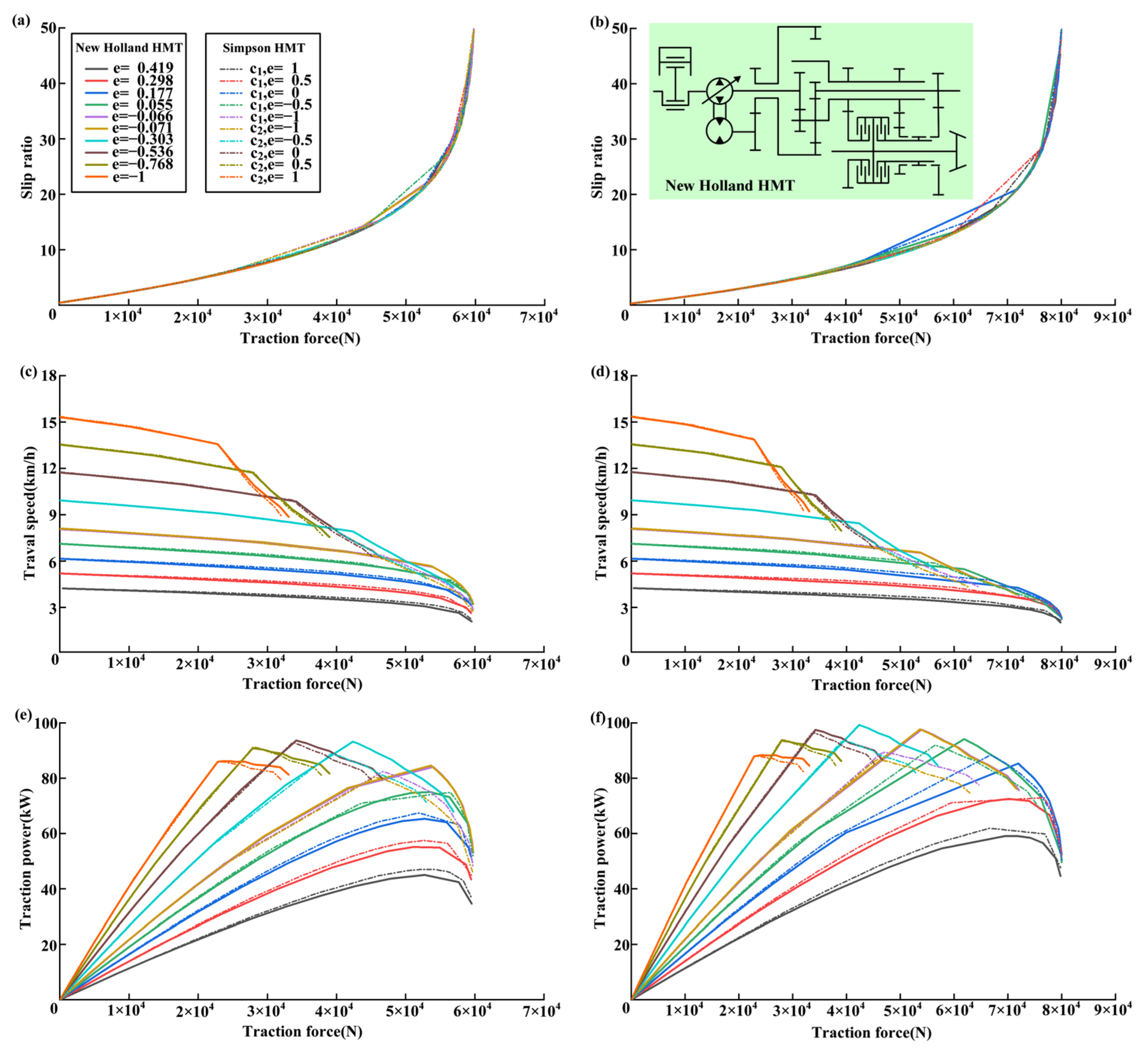
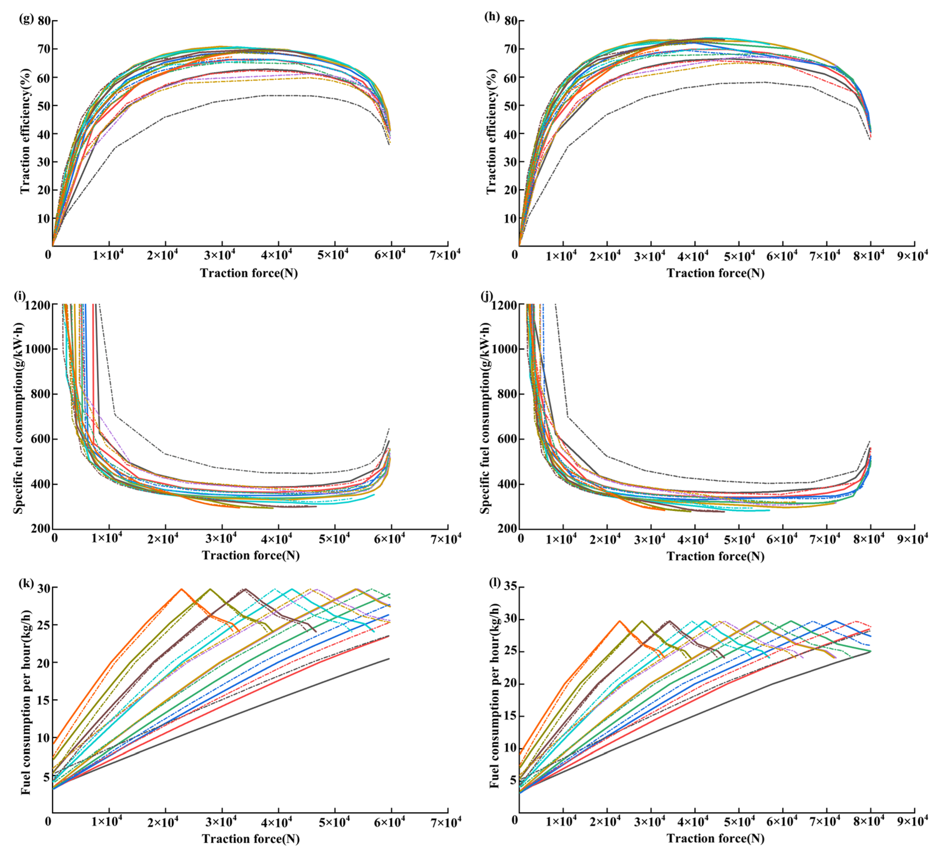
Figure 6 presents a performance comparison between the Simpson HMT tractor and the New Holland 2Z-X (B) HMT tractor. Due to optimizations implemented in both models, their overall performance exhibits minimal differences. The sole significant distinction occurs during the start-up phase, when tractor speed is very low. At this stage, New Holland’s displacement ratio ($e$ = 0.419) is smaller than that of the Simpson HMT ($e$ = 1) under the same speed conditions. This results in lower hydrostatic splitting power and higher traction efficiency for New Holland tractor, thereby reducing fuel consumption. However, this start-up phase is not the primary operating condition for tractors. As the tractor speed increases to reach working speeds, the performance of the Simpson HMT tractor improves rapidly. In some cases, its traction power and fuel consumption are both superior to those of New Holland tractors.

3.4. Discussion

3.4.1. Parameter Sensitivity

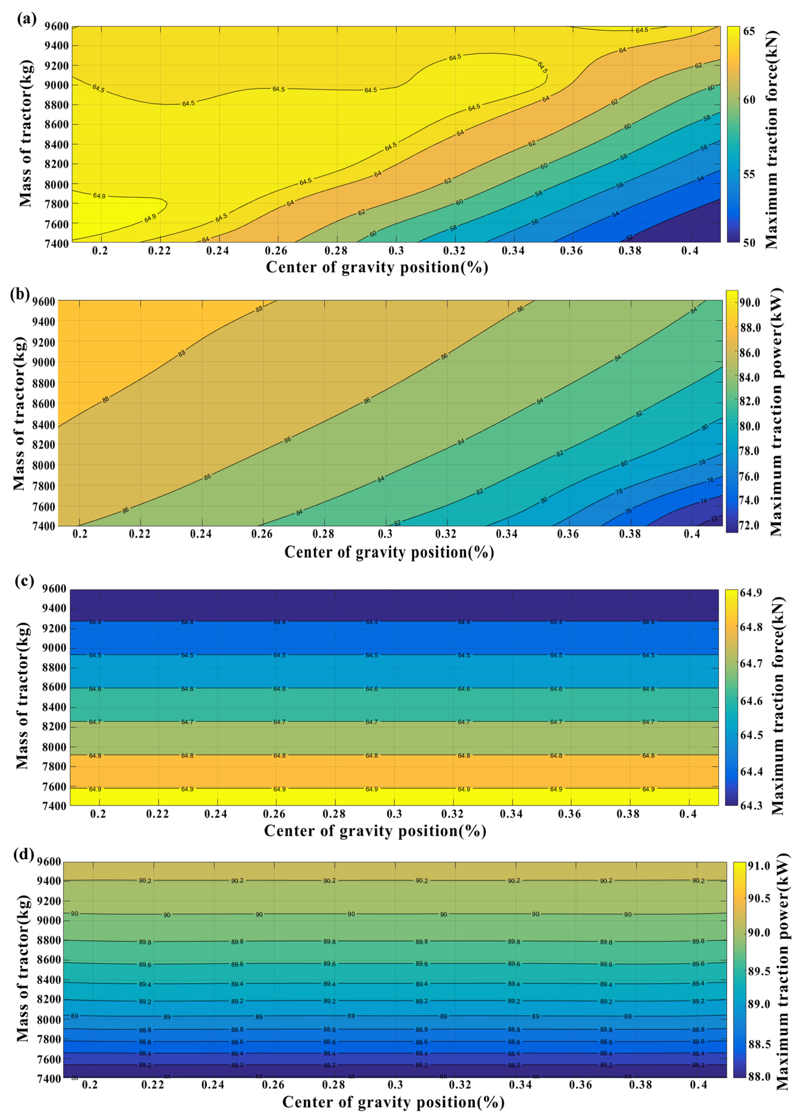
When tractors are equipped with different farm tools for operation, they exhibit varying masses and center of gravity positions (represented by $a/L\times 100\mathrm{\%}$). Figure 7 illustrates the impact of these two parameters on tractor traction performance. In two-wheel-drive mode, an increase in mass and a rearward shift in the center of gravity result in greater maximum traction force and traction power. However, when the maximum traction force exceeds 64 kN, the influence of mass and center of gravity position on traction performance becomes complex. This is because traction performance calculations cease at the engine speed corresponding to maximum torque (1500 r/min), at which point the slip rate has not yet reached its upper limit. In four-wheel-drive mode, the effect of center of gravity position on traction performance is not significant; instead, both maximum traction force and maximum traction power increase with increasing mass.

3.4.2. Farm Tools Matching Capability

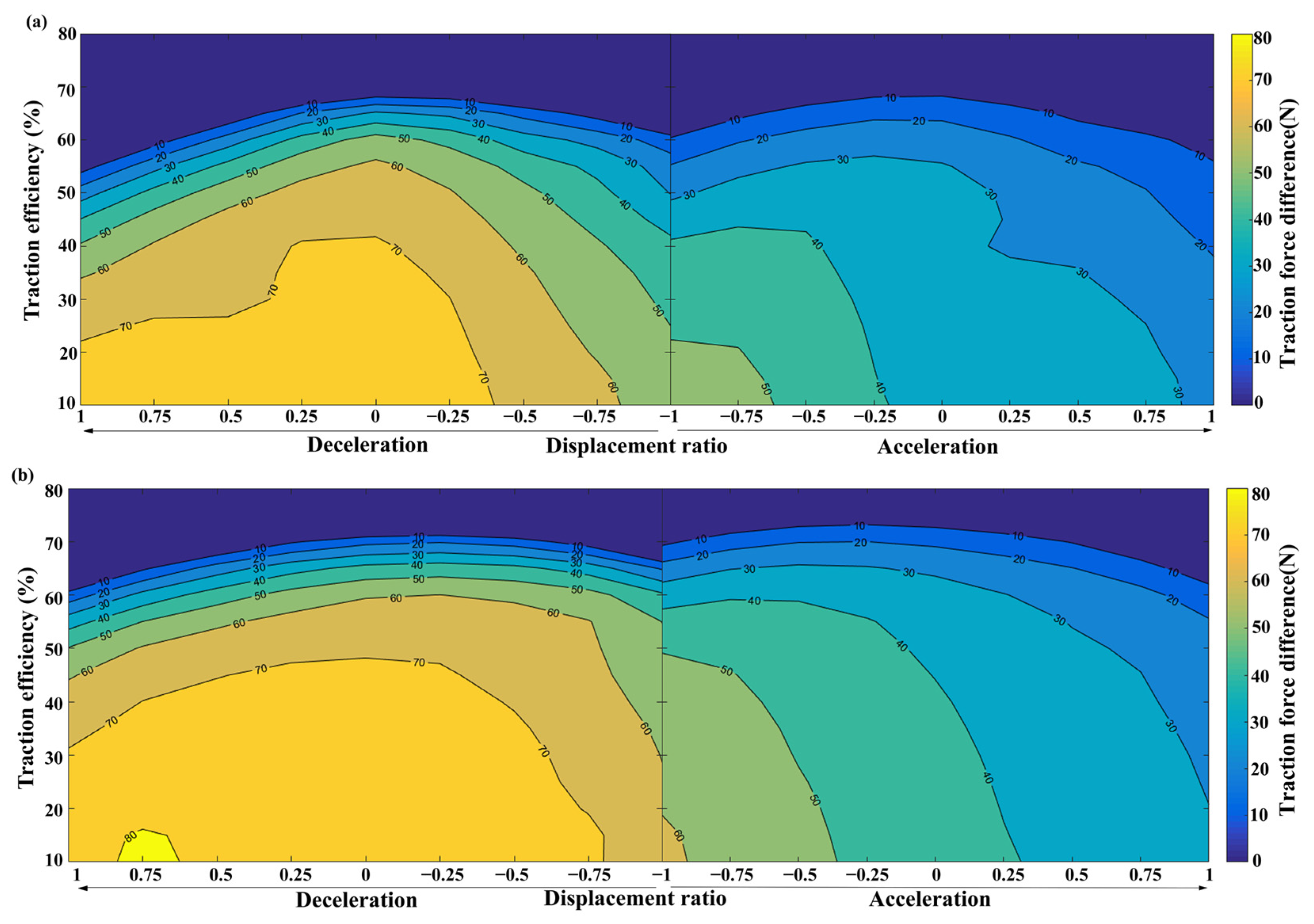
An important application of tractor traction performance is to evaluate its farm tools matching capability. Figure 8 shows the farm tools matching capability map of the HMT tractor under four-wheel-drive mode during standard road. The horizontal axis represents the HMT displacement ratio of the pump to motor, while the vertical axis represents the tractor traction efficiency. The contour values represent the range of traction force corresponding to tractor speed and traction efficiency (the difference between maximum and minimum traction force). A larger traction force difference means that the HMT tractor can be matched with more types or specifications of farm tools.

It is noted that there is an upper limit to the traction efficiency of the tractor at each speed, resulting in missing data in some high-efficiency regions shown in the figure. These data can only be obtained through interpolation, which may not have practical significance, but is crucial for demonstrating macroscopic patterns. As shown in the figure:

(1)

Due to the difference in transmission efficiency at the shift point ($e=1$) between ranges HM₁ and HM₂ of the HMT, the traction force difference in the tractor is staggered. In most cases, the traction force difference in range HM₂ is lower than that in range HM₁ under the same traction efficiency of the tractor. This is because range HM₂ has parasitic power on the low-speed side, and its transmission efficiency is lower than that of range HM₁ on the high-speed side without parasitic power.

(2)

Under the same tractor traction efficiency, the traction force difference should decrease as the tractor speed increases. However, the transmission efficiency of the HMT significantly disrupts this pattern, especially in the HM₁ range when the displacement ratio e changes from 1 to 0, the hydrostatic power portion of the HMT gradually decreases, and the transmission efficiency gradually increases, offsetting the negative impact of tractor speed on the traction force difference.

(3)

After optimizing the energy consumption of the HMT, the traction force difference in the tractor under various working conditions is been improved. It can be clearly observed that the optimized traction force difference not only exceeds 80 kN, but also the boundary range of each traction force difference in the map has expanded outward.

Obviously, the efficiency optimization of the HMT not only enhances the traditional tractor traction performance indicators, but also improves the ability of continuously variable tractors to match implements with high traction efficiency.

4. Conclusions

Currently, there are still few studies on the theoretical analysis of the traction performance of HMT tractors, and a systematic methodological framework has not yet been established, which brings some challenges to the development of continuously variable tractors. To address this issue, this study investigates the traction performance of an HMT tractor based on a Simpson configuration. The main work and conclusions are as follows:

(1)

A modeling approach for predicting the traction performance of HMT tractors is proposed, comprising two key sub-models: an energy consumption calculation model and a traction performance calculation model. By integrating these two sub-models in AMESim, the full set of traction performance data for the continuously variable tractors can be obtained through mathematical iterative calculations. The proposed model is based on a series of engineering-validated equations and shows good platform independence, with consistent results across different simulation environments.

(2)

The energy consumption optimization of the HMT has a pronounced influence on the traction performance of the continuously variable tractor, improving its transmission performance while reducing fuel consumption. Therefore, energy consumption optimization of the HMT plays a crucial role in tractor design and deserves sufficient attention. Previous work by the authors indicates that both the configuration and parameter settings affect the energy consumption of the HMT. In this study, the energy consumption optimization of the HMT is achieved by adjusting the transmission ratio of the gear pair ahead of the hydraulic pump.

(3)

The traction performance of the HMT tractor under four-wheel-drive mode is superior to that under two-wheel-drive mode, which is self-evident and therefore not discussed in detail here. In both drive modes, the effect of HMT energy consumption optimization on traction performance follows the same trend.

(4)

Road conditions significantly impact traction performance. When applying calculated traction performance results, the allowable slip rate should be specified based on the operating road. For standard roads, a lower allowable slip rate (e.g., 10%) is recommended, while higher values (e.g., 30%) may be appropriate for field conditions such as wheat stubble fields.

(5)

The starting method of the Simpson HMT tractor differs from that of the commercial New Holland 2Z-X (B) HMT tractor. The Simpson HMT tractor initiates operation through a hydrostatic range, whereas the New Holland 2Z-X (B) HMT tractor starts via a hydrostatic power-split range. At starting speeds, the New Holland tractor exhibits superior traction performance. However, at normal operating speeds, the Simpson HMT tractor exhibits higher traction power and lower fuel consumption in certain situations.

(6)

The traction performance of HMT tractor in two-wheel-drive mode is significantly affected by the tractor mass and its center of gravity position, while in four-wheel-drive mode, only the tractor mass affects the traction performance.

(7)

The benefits brought by energy consumption optimization are also reflected in farm tools matching capability. Lower HMT energy consumption enables the tractor to operate more types and specifications of farm tools at higher traction efficiency.

Although this study conducted a detailed analysis of the traction performance of HMT tractors, it has the following limitations:

(1)

Different roads exhibit not only varying rolling resistance coefficients but also distinct featured slip rates and driving force coefficients. In fact, these factors are also influenced by the type and size of tires. However, due to the lack of publicly available road data required for calculations, a comprehensive analysis of road types beyond standard roads and wheat stubble fields in northern China is not feasible.

(2)

Although the energy consumption model of HMT and the equations used for calculating tractor traction performance have been experimentally validated, experimental verification of their integrated models has not been conducted.

When implementing the model described in this study in practical applications, the potential impact of the aforementioned limitations should be taken into account. To address these shortcomings, future research should involve calibrating the calculation parameters under a broader range of road conditions and conducting comprehensive experimental verification of the traction performance calculation model for the HMT tractor.

References

1. Zhang, M.; Wang, N.; Zhou, S. Research on Fuel Economy of Hydro-Mechanical Continuously Variable Transmission Rotary-Tilling Tractor. Energies 2025, 18, 1490. [Google Scholar] [CrossRef] [Scilit]
2. Xi, Z.; Luo, Z.; Cao, F.; Niu, L.; Xu, L. Output speed control for hydro-mechanical continuously variable transmission of tractor. PLoS ONE 2024, 19, e0308493. [Google Scholar] [CrossRef] [Scilit] [PubMed]
3. Lu, K.; Liang, J.; Liu, M.; Lu, Z.; Shi, J.; Xing, P.; Wang, L. Research on Transmission Efficiency Prediction of Heavy-Duty Tractors HMCVT Based on VMD and PSO–BP. Agriculture 2024, 14, 539. [Google Scholar] [CrossRef] [Scilit]
4. Zhu, Z.; Hou, R.; Zhang, H.; Wang, D.; Chen, L. Multi-objective optimization of design parameters for tractor hydro-mechanical continuously variable transmissions. Sci. Rep. 2025, 15, 13261. [Google Scholar] [CrossRef] [Scilit] [PubMed]
5. Wang, J.; Xia, C.; Fan, X.; Cai, J. Research on Transmission Characteristics of Hydromechanical Continuously Variable Transmission of Tractor. Math. Probl. Eng. 2020, 2020, 6978329. [Google Scholar] [CrossRef] [Scilit]
6. Blumenthal, U.; Hansen, T.; Hartmann, R.O. Claas CVT Development for Different Applications in Commercial Vehicles. In Proceedings of the International Off-Highway & Powerplant Congress & Exposition, Milwaukee, WI, USA, 11–13 September 2000. [Google Scholar] [CrossRef] [Scilit]
7. Zhou, H.; Lu, Z.; Cheng, Z. Optimization of Transmission Parameters for a Tractor Equipped with HMCVT Based on Power Flow Analysis to Improve Efficiency. Appl. Sci. 2026, 16, 1641. [Google Scholar] [CrossRef] [Scilit]
8. Xia, Y.; Sun, D.; Qin, D.; Zhou, X. Optimisation of the power-cycle hydro-mechanical parameters in a continuously variable transmission designed for agricultural tractors. Biosyst. Eng. 2020, 193, 12–24. [Google Scholar] [CrossRef] [Scilit]
9. Cheng, Z.; Lu, Z. Research on HMCVT Parameter Design Optimization Based on the Service Characteristics of Agricultural Machinery in the Whole Life Cycle. Machines 2023, 11, 596. [Google Scholar] [CrossRef] [Scilit]
10. Li, J.; Zhao, Y.; Zhai, Z.; Han, B.; Du, Y.; Wang, L.; Zhu, Z. Research on Design and Analysis Method of the Double Planetary HMCVT Based on High Efficiency Transmission. Agriculture 2022, 12, 1958. [Google Scholar] [CrossRef] [Scilit]
11. Renius, K.T. Fundamentals of Tractor Design, 1st ed.; Springer Nature: Cham, Switzerland, 2020. [Google Scholar]
12. Ince, E.; Guler, M.A. On the advantages of the new power-split infinitely variable transmission over conventional mechanical transmissions based on fuel consumption analysis. J. Clean. Prod. 2020, 244, 118795. [Google Scholar] [CrossRef] [Scilit]
13. Wang, G.; Zhao, Y.; Song, Y.; Xue, L.; Chen, X. Optimizing the fuel economy of hydrostatic power-split system in continuously variable tractor transmission. Heliyon 2023, 9, e15915. [Google Scholar] [CrossRef] [Scilit] [PubMed]
14. D’Andrea, D.; Risitano, G.; Alberti, F. Fuel Consumption Reduction and Efficiency Improvement in Urban Street Sweeper Using Power Split with Lockup Clutch Transmission. Appl. Sci. 2022, 12, 10160. [Google Scholar] [CrossRef] [Scilit]
15. Rossetti, A.; Macor, A.; Benato, A. Impact of control strategies on the emissions in a city bus equipped with power-split transmission. Transp. Res. D Transp. Environ. 2017, 50, 357–371. [Google Scholar] [CrossRef] [Scilit]
16. Siddique, M.A.; Baek, S.M.; Baek, S.Y.; Jeon, H.H.; Park, J.D.; Park, M.J.; Yang, C.W.; Park, M.J.; Kim, Y.S.; Kim, W.S.; et al. Effect of motor speeds on traction performance of a single-motor electric tractor at various gear stages during plow tillage. Sci. Rep. 2025, 15, 26590. [Google Scholar] [CrossRef] [Scilit] [PubMed]
17. Brennensthul, M.; Czarnecki, J.; Bialczyk, W. Assessment of Tractor Tires Used in Forest Conditions in Terms of Traction Performance and Impact on Ground. Croat. J. For. Eng. 2024, 45, 97–113. [Google Scholar] [CrossRef] [Scilit]
18. Rao, Z. Design of Planetary Gear Transmission, 2nd ed.; Chemical Industry Press Co., Ltd.: Beijing, China, 2019. [Google Scholar]
19. Liu, F. Design and Characteristics Research on the Hydro-Menchanical Continuously Variable Transmission of High-Power Tractors. Master’s Thesis, Nanjing Agricultural University, Nanjing, China, 2015. [Google Scholar]
20. Zhang, W.; Fang, Z. Mathematical Model and Computer Plotting Program for Theoretical Traction Performance Curves. Tractor 1987, 1987, 23–28. [Google Scholar]
21. Zhou, Z.; Fang, Z.; Zhang, W. Computer Aided Analysis on the Theoretical Tractive Characteristics of Tractor. J. Luoyang Inst. Technol. 1993, 14, 1–6. [Google Scholar] [CrossRef] [Scilit]
Figure 1. Schematic diagram of the HMT system.
Applsci 16 06979 g001
Figure 2. Experimental verification of energy consumption model.
Applsci 16 06979 g002
Figure 3. Calculation model for traction performance of HMT tractors.
Applsci 16 06979 g003
Figure 4. Tractor traction performance on standard road: (a) slip rate under two-wheel drive; (b) slip rate under four-wheel drive; (c) travel speed under two-wheel drive; (d) travel speed under four-wheel drive; (e) traction power under two-wheel drive; (f) traction power under four-wheel drive; (g) traction efficiency under two-wheel drive; (h) traction efficiency under four-wheel drive; (i) specific fuel consumption under two-wheel drive; (j) specific fuel consumption under four-wheel drive; (k) fuel consumption per hour under two-wheel drive; (l) fuel consumption per hour under four-wheel drive.
Applsci 16 06979 g004aApplsci 16 06979 g004b
Figure 5. Tractor traction performance on wheat stubble field: (a) slip rate under two-wheel drive; (b) slip rate under four-wheel drive; (c) travel speed under two-wheel drive; (d) travel speed under four-wheel drive; (e) traction power under two-wheel drive; (f) traction power under four-wheel drive; (g) traction efficiency under two-wheel drive; (h) traction efficiency under four-wheel drive; (i) specific fuel consumption under two-wheel drive; (j) specific fuel consumption under four-wheel drive; (k) fuel consumption per hour under two-wheel drive; (l) fuel consumption per hour under four-wheel drive.
Applsci 16 06979 g005
Figure 6. Tractor traction performance on New Holland HMT: (a) slip rate under two-wheel drive; (b) slip rate under four-wheel drive; (c) travel speed under two-wheel drive; (d) travel speed under four-wheel drive; (e) traction power under two-wheel drive; (f) traction power under four-wheel drive; (g) traction efficiency under two-wheel drive; (h) traction efficiency under four-wheel drive; (i) specific fuel consumption under two-wheel drive; (j) specific fuel consumption under four-wheel drive; (k) fuel consumption per hour under two-wheel drive; (l) fuel consumption per hour under four-wheel drive.
Applsci 16 06979 g006aApplsci 16 06979 g006b
Figure 7. Influence of mass and center of gravity position on tractor traction performance: (a) maximum traction force under two-wheel drive; (b) maximum traction power under two-wheel drive; (c) maximum traction force under four-wheel drive; (d) maximum traction power under four-wheel drive.
Applsci 16 06979 g007
Figure 8. Farm tools matching capability map of the continuously variable tractor: (a) traction efficiency difference in tractors before HMT optimization; (b) traction efficiency difference in tractors after HMT optimization.
Applsci 16 06979 g008